
Modeling of Solid and Bio-Fuel Combustion Technologies
Arafat A. Bhuiyan, Md. Rezwanul Karim and Jamal Naser, Faculty of Science, Engineering and Technology (FSET), Swinburne University of Technology, VIC, Australia
Inefficient process in the thermal power station leads to greenhouse gas emission. Reductions in emissions are largely dependent on the improvement of efficiency, with lower fuel consumption as a 1% improvement in power station efficiency delivering an almost 3% reduction in CO2 emissions. Maximum CO2 reduction is also possible through the use of alternative fuels and CO2 capture. Therefore, there is a need for energy-efficient technology to improve power plants that are able to utilize alternative fuels and CO2 capture. Coal is a major source of fuel, while biomass fuels, such as energy crops, waste wood, and agricultural residues are supplementary. The design, operation, and maintenance of combustion equipment require detailed understanding of the combustion process inside the furnace. In order to explore the major challenges, experimental methods are important but often inadequate to analyze the detailed phenomena inside the boiler, especially for industrial furnaces. A computational technique provides the opportunity to investigate in detail, the combustion phenomena and contaminant development inside the furnace. In order to understand combustion-related issues and problems for direct firing or packed bed combustion, modeling and analysis are required. This chapter will briefly report the recent advances in the combustion technologies, different carbon capturing and storage systems, modeling methodology for coal combustion, biomass co-combustion, packed bed combustion, and slag formation modeling. Also, examples of coal/biomass combustion will be illustrated to investigate, in detail, the combustion phenomena and related issues in the furnace.
Keywords
CO2 capture; coal/biomass combustion; co-firing; slagging; packed bed modeling; computational fluid dynamics (CFD); radiation heat transfer; energy efficiency; carbon in ash (CIA)
11.1 Introduction
In general, much effort is currently focused on reducing greenhouse gas (GHG) emissions from fuel-fired power generation. The efficiency of a thermal power station has a key influence on its GHG production. Improving efficiency leads to significant reduction in emissions and fuel consumption. An analysis shows that a 1% improvement in power station efficiency delivers almost a 3% reduction in CO2 emissions. Based on this framework, the retrofitting and/or replacement of existing fuel-fired power plants with new-technology generation capacity can provide a better greenhouse advantage. Clean coal technologies are commonly used to define a range of technologies from high-efficiency generation systems to the ultimate, zero-emission power production. As coal will remain a considerable part of the energy mix in the foreseeable future, so clean coal technologies allow more electricity to be produced from less coal. This will play a significant part in efficiency gains in electricity generation. Also, efficiency improvements include the most cost-effective and shortest lead time actions for reducing emissions from coal-fired power generation. This is particularly the case in developing countries where existing power plant efficiencies are generally lower and coal use in electricity generation is increasing. Improving the efficiency of pulverized coal-fired power plants has been the focus of considerable efforts by the coal industry. This increases the performance of carbon capture and storage programs and decreases the associated economic costs. In addition, efficiency gains can also be made by developing innovative ways to generate electricity from coal or reducing the amount of energy.
Besides the use of coal in power plants, combustion technologies can be enhanced to further decrease the total costs of heat and/or power produced and to maximize the safety and simplicity of operations. The need for innovation is also driven by the wish to burn new biomass fuels, such as energy crops, waste wood, and agricultural residues. Co-firing biomass with coal in traditional coal-fired boilers is becoming increasingly popular, as it capitalizes on the large investment and infrastructure associated with the existing fossil-fuel-based power systems while traditional pollutants (SOx, NOx, etc.) and net GHG (CO2, CH4, etc.) emissions are decreased. On the other hand, combustion in a packed bed or fixed bed has now become a recent topic of interest for biomass combustion. The design, operation, and maintenance of such combustion equipment require a detailed understanding of the burning process inside the bed. There have been many researches into packed bed combustion of solid fuels, mainly biomass and wastes during the last two decades. However, the commercial application of a packed bed biomass combustion system in a furnace as yet is very limited due to insufficient knowledge on combustion mechanisms and processes. It does have a great deal of potential as a system of biomass combustion which can improve the combustion efficiency and meet more stringent government emission regulations expected in the future.
Experimental investigation is considered the most appropriate method for such study. But an experiment is not only an expensive and lengthy process but also technically challenging and it sometimes interrupts the regular operation of plants. Therefore, experimental methods are important but often inadequate to analyze the detailed phenomena inside the boiler, especially for an industrial furnace. Lab-scale analysis was another supplementary method which is extensively accepted in order to solve this type of problem. There remain, however, some limitations in the lab-scale compared to full-scale analysis based on different parameters and related physics. Detailed information of different processes and reactions inside the furnace, combustion phenomena, predicting the flue gas emissions, mixing, gaseous reactions, surface combustions, and paths of particles are not possible to trace in experimental investigations. Knowledge about the performance of coal/biomass combustion, its emission, firing, ashing, slagging, and fouling is still quite limited. Instead of performing expensive and time-consuming test runs, modeling is increasingly used to calculate flow, temperature, and residence time distributions as well as two-phase flows (flue gas and ash particles) in coal/biomass furnaces and boilers, and to evaluate the impact of design on combustion quality and emissions. Computational technique provides the opportunity to investigate in detail the combustion phenomena and contaminant development inside the furnace. However, the success of computational analysis largely depends on the proper numerical technique and the physical/chemical models employed. In order to gain a deep understand of combustion-related issues and problems for direct firing or packed bed combustion, modeling and analysis are a must. But modeling of the different types of issues in the combustion process requires theoretical as well as numerical knowledge.
This chapter will briefly demonstrate the recent advances in combustion technologies, different carbon-capturing and storage systems, applications of modeling in combustion technologies including coal combustion, biomass co-firing, packed bed combustion, and slag formation modeling. A number of modeling cases will be illustrated to investigate in detail, the combustion phenomena and contaminant development inside the furnace, considering small-scale and large-scale coal biomass combustion.
11.2 Different Carbon Capture Technologies
In order to understand the technologies that are used for CO2 capture in conventional power plants, it is important to understand the systems of leading technology for these power plants. The three main techniques, which have been developed for CO2 capture from these different systems of leading technology, are precombustion capture, postcombustion capture, and capture of oxy-fuel combustion as presented in Figure 11.1. The precombustion capture technique extracts CO2 from the fuel before the burning process in the combustion chamber. The postcombustion capture technique involves capturing CO2, as well as reducing particulate matter SOx and NOx in the combustion flue gases. The oxy-fuel combustion technique captures carbon dioxide from the flue gases of combustion. It is similar to the postcombustion capture technique in terms of separating the CO2 from the exhaust gases as a final process of sequestration, but it is less chemically complicated. Details about the advancements in CO2 capture technology are given in Ref. [2]. In short, these three CO2 capture technologies have different outcomes, particularly with regard to reduction of power plant efficiency and in increasing the cost of electricity production. Advantages and disadvantages of different CO2 capture approaches are illustrated in Table 11.1.
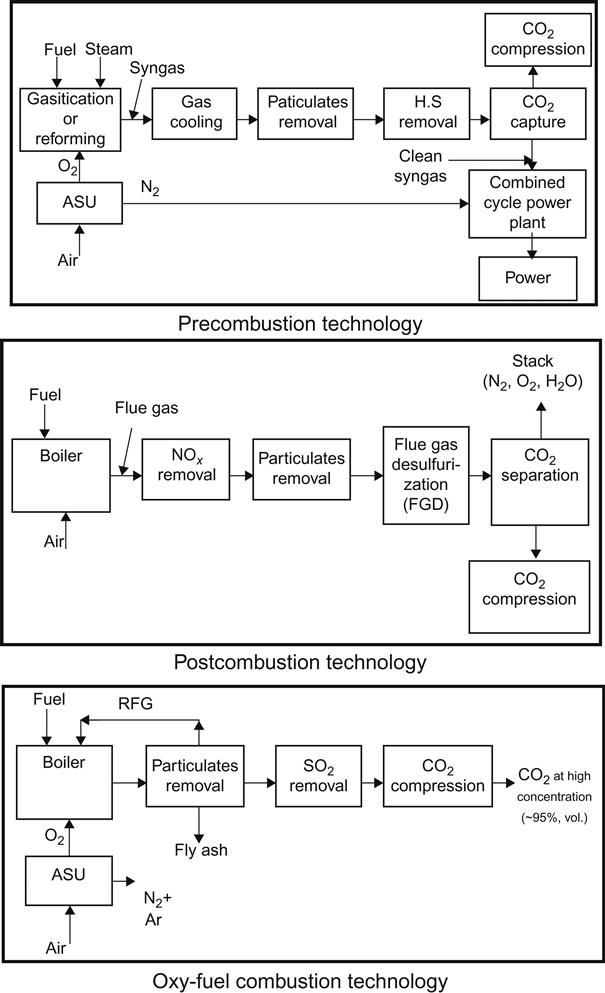
Table 11.1
Advantages and disadvantages of different CO2 capture approaches [2]

Among all the carbon capture technologies, oxy-fuel combustion is a GHGs abatement technology in which coal is burned using a mixture of O2 and recycled flue gas (RFG), to obtain a rich stream of CO2 ready for sequestration [3]. This carbon capture technology has been considered as one of the most effective technologies to reduce gaseous emissions. In general, the conventional boiler uses air as an oxidizer in the combustion process, hence nitrogen is the main component in the flue gas as its concentration in air is approximately 79% by volume. In oxy-fuel combustion, air is replaced with oxygen and RFG mixture. The flue gas produced in oxy-fuel combustion has very high concentration of CO2 compared with the flue gas achieved in air combustion, and is ready for sequestration. The basic schematic of oxy-fuel combustion with the RFG is presented in Figure 11.2. Recycled ratio (RR) is the most significant parameter in an oxy-fuel system when operated with RFG. It is a function of the recycled gas mass flow rate, mRFG (kg s−1) and the product gas mass flow rate, mPFG (kg s−1). Product flue gas (PFG) is the amount of flue gas produced within the furnace due to combustion. As CO2 has higher specific heat capacity compared to N2, the oxy-fuel combustion flame has different radiative characteristics compared to air-fired flame, so the use of oxy-fuel combustion technology leads to many changes in the furnace [5,6]. The RR can be defined as follows:
(11.1)

11.3 Status of Coal/Biomass Combustion Technology
Combustion of fossil fuels is a proven thermochemical conversion technology for heat and power production which is connected with the formation of pollutants, also a source of deterioration of the global environment. Coal is a major source of fossil fuel, responsible for generating electrical energy globally [7]. Also, combustion of coal results in the emission of GHGs, the accumulation of which in the atmosphere since the start of the Industrial Revolution has been contributing to climate change [8]. Based on this concern, international efforts, like the Kyoto protocol, call for the reduction of emissions, especially CO2, from industrialized countries. For the reduction of CO2 emissions from coal-fired power plants, a number of CO2 capture technologies can be implemented for continuing the use of fossil fuels, as discussed earlier. Apart from these processes, different separation techniques are also suggested, such as gas phase separation, absorption, adsorption, and hybrid processes. Recent developments in the CO2 capture technologies include some innovative concepts (i.e., calcium looping (CaL), chemical looping, and amines scrubbing systems) that have been suggested in the literature. CaL, a post-combustion capture technology, is suggested as a competitive concept for CO2 reduction technique [9] for power plants. CaL is achieved by oxy-firing for the capturing of CO2-rich flue gas which is absorbed by CaO and CaCO3 in a carbonator. However, this technique has relatively high energy consumption. The ECO-Scrub combustion concept [6], a combination of partial oxy-fuel combustion and postcombustion capture, provides comparatively higher efficiency than only the postcombustion process. Another important concept is chemical looping combustion (CLC). In CLC, a high-purity and concentrated CO2 stream is produced as there is no contact between the fuel and the air as metal oxide works as transportation media for O2. Hence, lower energy is required compared to other CO2 separation processes.
In recent years, many efforts have been devoted to the development of oxy-fuel coal combustion. From pilot-scale and laboratory-scale experimental studies, oxy-fuel combustion has been found to differ from air combustion in several ways, including reduced flame temperature, delayed flame ignition and reduced GHG emissions [8]. Several small-scale experimental studies have been conducted at various combustor designs. A 20-KW down-fired coal combustor was considered by Liu et al. [10] using the coal in air and in oxy coal environment. Significant differences were observed in the char burnouts and gas temperatures in the oxy-fuel combustion case. Another study considering an entrained flow reactor was used in Ref. [11] to investigate experimentally the ignition and burnout of coals under oxy-fuel conditions. The ignition temperature of the individual coals showed a strong dependence on the composition of the atmosphere. The burnouts of the samples with a mixture of 79% CO2–21% O2 are lower than those conducted in air. When the O2 in the mixtures is improved to a value of 30%, the burnout is higher than in air. Suda et al. [12] conducted the experimental study in a chamber considering different kinds of coal particles to investigate the effect of carbon dioxide (CO2). Another experimental study for the firing of dry lignite under an O2-enriched environment in a 0.5-MW test facility has been conducted by Kaß et al. [13], focusing on the flue gas compositions in air and oxy-fuel combustion conditions.
Natural resources, such as oil and gas, are likely to be limited within this century according to the literature [14,15]. Renewable energy, together with fossil energy, are the main energy sources on the earth. Table 11.2 shows a global renewable energy scenario for 2040, claiming that by then nearly half of the global energy supply will come from renewable energy [16]. Today biomass is seen as the most promising energy source to mitigate GHG emissions. Combustion of biomass is the most suitable and economical way to utilize biomass energy. It is responsible for over 97% of the world’s bioenergy consumption [17]. Understanding the characteristics of biomass and the interactions in combustion facilities is important. Biomass fuels have a wide range of different physical and chemical properties. Suitability of biomass fuel and the type of combustion facilities employed is mainly based on the physical properties of biomass fuel. On the other hand, chemical properties affect the proximate and ultimate analysis of the biomass fuel. There are a total of 62 countries in the world currently producing electricity from biomass. The United States is the dominant biomass electricity producer at 26% of world production, followed by Germany (15%), Brazil, and Japan (both 7%) [18].
Table 11.2
Global renewable energy scenario by 2040
| Contributions | Year | ||||
| 2001 | 2010 | 2020 | 2030 | 2040 | |
| Total consumption (million ton oil equivalent) | 10,038 | 10,549 | 11,425 | 12,352 | 13,310 |
| Biomass | 1080 | 1313 | 1791 | 2483 | 3271 |
| Total renewable energy sources | 1365.5 | 1745.5 | 2694.4 | 4289 | 6351 |
| Renewable energy contribution (% sources) | 13.6 | 16.6 | 23.6 | 34.7 | 47.7 |

11.4 Modeling of Coal/Biomass Combustion
11.4.1 Fundamentals of Combustion Modeling
It is important to be able to accurately calculate and predict the temperature levels, turbulent flow fields, species concentrations, and emission levels from combustion equipment, especially with the present concerns about GHG emissions. As combustion consists of complex carbon–oxygen reactions, Devolatilization and char oxidation are expressed in the form of homogeneous and heterogeneous reactions. The suitability of multistep chemical reactions (one, two, and three steps) is discussed by several authors. The limitation of the global power law is its dependence on temperature and oxygen partial pressure to the order of char reaction rate and CO/CO2 production rate. To illustrate the applications of combustion modeling in computational fluid dynamics (CFD), it is important to define all the mathematical models that relate to this combustion phenomenon. The details of the model are described below.
Gas/particle phase model: In gas phase modeling, three-dimensional (3-D) nonsteady-state Eulerian partial differential conservation equations (PDEs) are used for multicomponent gaseous phase. The general form of Eulerian transport equation is [4]:
(11.2)
In the particulate phase model, the discrete droplet method [19] is generally considered. This method includes the momentum exchange, heat, and mass transfer phenomena. The differential equation for a solid particle is defined as follows:
(11.3)
where
(11.4)
(11.5)
(11.6)
For spherical-shaped particles, drag is simple. But for irregular-shaped particle flow, the aerodynamics of the fuel particle is largely dependent on the deviation of shape. From the various formulations in literature for the drag coefficient, the drag coefficient for spherical- and irregular-shaped coal particles uses the following formulation, respectively [20].
(11.7)
 (11.7)
(11.8)
(11.9)
(11.10)
(11.11)
(11.12)
where, ![]() ,
, ![]() ,
, ![]() , and
, and ![]() are functions of the shape factor, f.
are functions of the shape factor, f.
Coal combustion models: The Eddy Breakup (EBU) model, one of the important turbulence controlled combustion models, is applied for combustion modeling. This model determines whether O2 and fuel are in limiting conditions and the reaction possibility. In this model, the mean reaction rate is an important parameter which is defined as follows:
(11.13)
Two very important terms in the modeling of coal combustion are devolatilization and char oxidation. These processes are complex. The volatile production rate is defined as:
(11.14)
(11.15)
Char oxidation is the secondary phase of particle combustion after the devolatilization. Char combustion can be modeled with the global power-law [21]. When the devolatilization is complete, the remainder is char and ash. This char will react with the gases steadily. The diffusion of O2 is responsible for the oxidation rate of char particles. This is treated as a suitable model compared to other models [22]. The rate of char oxidation per unit area is KcPs, where the value of Kc can be written as:
(11.16)
Turbulence model: A number of turbulence models are available to consider the flow ranges. Among them, the k–ɛ is a commonly accepted model for turbulence modeling, especially for industrial applications, and is available in most CFD codes.
Turbulent kinetic transport equations:
(11.17)
Rate of dissipation of energy from the turbulent flow:
(11.18)
(11.19)
Heat transfer models: Radiative heat transfer is an important phenomenon in combustion modeling, considering emission [23]. Most of the proposed models for radiative heat transfer modeling fall under the category of weighted-sum-of-gray-gases models [24]. The radiative heat transfer modeling can be achieved using the discrete transfer radiation method (DTRM). In DTRM, the radiation transfer equation (RTE) is solved for the calculation of radiation phenomena. In this method, the radiation intensities are defined assuming a single ray with constant temperature where the emissivity totally depends upon the local temperature and gas composition [25]. In modeling coal combustion, convection and radiation heat transfer are counted during the particle and gas interactions in the furnace. The convective and radiative heat transfers are defined as:
(11.20)
(11.21)
11.4.2 Recent Numerical Activities in Combustion
Several numerical attempts have been made to computationally model the combustion in oxy-fuel environments in recent years [26–29]. Edge et al. [29], in their numerical study, investigated the effect of radiation to the furnace wall by using large eddy simulation and Reynolds-averaged Navier–Stokes-based governing equations. The flame properties were clarified for coal combustion in an air- and oxy-fired combustion test facility (CTF). Recently, Audai et al. [30–34] carried out comprehensive modeling for the combustion of pulverized dry lignite in lab-scale [30,32,33] and large-scale [31,34–36] furnaces under different combustion environments. The studies demonstrated the flame ignition changes and the ignition stability of coal flame in air and oxy-fuel combustion scenarios. The effects of SOx and NOx emission concentration have also been investigated. These numerical results showed that the flame temperature distributions and O2 consumptions in the oxy-fuel case were similar to the air combustion case for 25% O2 and 75% RFG.
CFD models for coal combustion have been developed based on the theoretical as well as experimental investigations, including all the stages of the combustion. The CFD modeling method for combustion of biomass particles is a significant challenge. There are still a very limited number of numerical simulations of pulverized biomass combustion using detailed combustion models. Many CFD studies made in relation to coal combustion have been modified to apply to biomass combustion. There are a number of available CFD models and codes. Only a few CFD attempts in biomass combustion in boilers and furnaces are found in the literature [37]. Since biomass is the only carbon-based renewable fuel, its application becomes more and more important for climate protection. Fundamentals, technologies, and primary measures for emission reduction in combustion and co-combustion of biomass are significant factors that must be considered in CFD [38]. Williams demonstrated that co-firing of biomass and coal can be beneficial in reducing the carbon footprint of energy production [39]. It is pointed out that for future improvements in furnace design, modeling can be useful as a tool to calculate flow distributions in furnaces and the reaction chemistry. A computational investigation of the special effects of co-firing biomass with coal is presented in the study [40] considering bituminous coal and wheat straw with a proportion of 10% and 20% (thermal basis). A similar study conducted by Yin et al. [41] presents a comprehensive study of co-firing wheat straw with coal in a 150-kW swirl burner reactor. A full-scale coal- and straw-fired utility boiler was modeled by Kaer et al. [42] using a commercial CFD code. The results showed a noticeable difference in the temperature, species concentration, etc. Devolatilization and burnout of the larger straw particles occurred further away from the burner mouth, which changed the combustion behavior.
A number of 3-D studies were conducted for the modeling of coal-biomass co-firing in large-scale furnace. 3-D mathematical modeling for co-combustion of paper sludge and coal in a fluidized bed boiler using a commercial software FLUENT has been developed [43]. Results indicate that paper sludge spouts into the furnace from the recycle inlet can increase the furnace maximum temperature. Using CFD simulations, a comparison of measurements for the well-defined conditions within a pilot-scale furnace co-firing coal and sawdust is given in Ref. [44] for the evaluation of wood co-firing injection strategies. Pallarés studied a CFD numerical analysis [45] of co-firing coal and Cynara carunculous in a 350-MWe utility boiler to determine the most influent operational factors related to the biomass feeding conditions such as biomass mean particle size, level of substitution of coal by biomass and feeding location in the furnace, identifying their influence in the combustion process. Axelbaum carried out a CFD analysis [46] to determine the cause of the increased NO conversion and to identify differences between air-fired and oxy-fuel co-fired flames in a 30-kW laboratory-scale test facility. It was addressed in the findings that co-fired flames have longer volatile-flame regions, which is influenced by the increased volatile fraction and particle size associated with the biomass.
Ghenai studied the effects of co-firing using CFD where coal was blended with 5–20% wheat straw on a thermal basis [47]. This investigation includes the prediction of volatile evolution and char burnout. One important result is the reduction of NOx and CO2 emissions when using co-combustion. This reduction depends on the proportion of biomass (wheat/straw) blended with coal. Gubba [48] carried out a numerical modeling of the co-firing of pulverized coal and straw in 300-MWe tangentially fired power generation plants. In this study, a particle heat-up model is applied to a co-firing coal/biomass simulation up to 12% thermal biomass loading. Karampinis investigated a 3-D numerical model for co-firing lignite and biomass in large-scale utility boilers of 300-MWe pulverized-fuel, tangentially fired boiler, operating with low-quality lignite considering the model for the nonspherical form of the biomass particle, which influences the drag coefficient and its devolatilization and combustion mechanisms [49]. Also, extensive CFD modeling was used to design the ROFA system and to locate the proper elevation for the biomass burners [50]. Though a number of models have been developed for co-firing in industrial furnaces, as found in recent literature, substantial progress is still required for the implementation of the co-firing concept in industrial power plants.
11.5 Modeling of Packed Bed Combustion
Combustion in a packed bed or fixed bed has now become a recent topic of interest for biomass and other solid fuel combustion [51,52]. A packed bed is a pile of fuel particles sitting on top of a grate (Figure 11.3). The most common mode of packed bed combustion is underfeed, where fuel is lit at the top and burns downward and airflow is from the bottom. Airflow must be sufficiently low so that the majority of the fuel particles do not become suspended in the flow creating a fluidized bed. Historically, this was the main means of burning coal, wood, coke, and charcoal in steam locomotives. Modern industrial applications include wood/wood waste combustion in pulp and paper plants, waste incineration, power generation, etc. In many applications, the combustor is batch-fed and a single charge of fuel is allowed to fully burnout before more fuel is added. A packed bed can be used to burn many different solid fuels, but chipped or pelletized biomasses are of recent interest.

Packed bed combustion can be of two types: stationary or moving. Stationary packed bed is more commonly used. Some grate-fired boilers use a moving bed combustion technique. The burning process of fuel inside the bed is very important to design, operation, and maintenance of the packed bed combustion systems. Comprehensive researches, both numerical and experimental work, are on-going to investigate the burning process of solid fuel combustion (biomass and wastes) in a packed bed over the last two decades. Experimental investigation is the most appropriate method to develop an efficient combustion system. However, due to the limited accessibility, inhomogeneity inside the packed bed, complex solid conversion mechanism, etc., it is difficult to obtain data by measurement in the packed bed. CFD modeling can be used to study combustion phenomena in detail by combining theoretical models and experimental data. Many variables of the process can be analyzed under different working conditions. It can also help to minimize the complications of experimental work by estimating the field values inside the whole domain and different places without disturbing the working condition of the system. There are a very limited number of numerical simulations of packed bed biomass combustion systems. A comprehensive model for efficient combustion of packed bed biomass considering both the solid and gas phase is currently in development.
11.5.1 Recent Numerical Models
The literature shows some complete reviews of packed bed combustion systems [54,55]. The authors reviewed the up-to-date knowledge on different packed bed furnaces burning biomass and other solid fuels, their firing system, the important combustion mechanism, the recent invention in the technology, the most demanding issues, the current research and development activities, and the important future problems to be resolved.
Combustion of solid fuel itself is a complex phenomenon because of the compound mechanisms and parameters involved. There are only a very few experimental investigations on packed bed biomass combustion. This is due to the limited accessibility and inhomogeneity inside the packed bed, which makes it difficult and complex to obtain information by measurements about the conversion processes in the packed bed. Ryu et al. [56] measured temperatures, species, and mass loss profiles of four different biomass types in a fixed bed under fuel-rich conditions. The combustion of straw in a fixed bed was experimentally investigated by Van der Lans et al. [57]. They measured temperatures in the packed bed at different heights and species concentrations above the bed. Porteiro et al. [53,58,59] measured the reaction front propagation rates of a fixed bed combustor. In a counter-current process the ignition front propagation velocity is experimentally studied for eight different biomass fuels with a wide range of origins, compositions, and packing properties [53]. A parametric analysis on influential parameters of ignition front propagation has also been conducted to examine a wide range of parameters from different biomasses [58]. An existing fixed-bed combustor is modified to study the structure of the reaction front thickness and its dependence on the air mass flow rate. The position of the bed surface is continuously measured [59].
CFD is an effective tool for the design and optimization of packed bed combustion. The review of elaborations on packed bed modeling published in the literature shows a broad variety of different model approaches to describe entire packed bed systems. According to the calculation of energy equation, these models are homogeneous and heterogeneous models (Table 11.3). In homogeneous models, the temperatures of the gas and of the solid phase are assumed to be equal and one overall energy balance equation is applied [57,60]. In heterogeneous models, the gas phase and the solid phase have individual energy equations [61,62]. When the temperature difference between the gas and solid is not negligible, which is the case for packed bed combustion, heterogeneous modeling is recommended.
Table 11.3
Classification of models according to energy equation
| Classification | Model | Description | References |
| Calculation of energy equation for solid and gas phase | Homogeneous | One overall energy equation applied | [57,60] |
| Heterogeneous | Individual equations | [61,62] | |
| Treatment of solid phase in heterogeneous models | Continuous | Both phases are distributed continuously over whole spacial domain | [63–66] |
| Discrete particle | Interparticle effects like momentum and energy exchange can be described | [67,68] |

Based on the treatment of the solid phase in the heterogeneous models, they can be classified into continuous models [63–66,69] and discrete particle models [67,68]. Continuous heterogeneous models treat both phases as if they are distributed continuously over the whole spacial domain. At each point in space both phases exist with distinguished properties. The common limitation of the continuous packed bed model is that the intraparticle effects cannot be described sufficiently. Additionally, it is very difficult to model the inter-particle interactions in the packed bed with a continuous model. The discrete particle model enhances the packed bed modeling by considering the packed bed as an ensemble of representative particles, where each of these particles undergoes thermal conversion processes. In this way the interparticle effects, e.g., momentum and energy exchanges, can be fully described.
The common modeling approach of a packed bed is to divide the simulation into the bed and the freeboard, although there is a strong coupling between them. Commercial CFD codes (Fluent, Star-CD, CFX, etc.) have been used to model the gas phase while the bed was simulated using separate models [61,70,71]. The bed and the freeboard are linked by a surface where mass and energy exchange occurs. This linking is considered one-directional by some authors [72,73], which means the solution of the bed and the freeboard are independent of each other. Other authors [74,75] have developed different bed model mechanisms and the differences in the solution of the freeboard are included in the simulation. It was assumed that homogeneous combustion of the gases in the combustion chamber generates a strong radiative flux which induces the biomass decomposition in the bed [76]. A zero-dimensional bed was modeled accounting for the main processes of the biomass conversion. To calculate various inputs of the gas phase model like gas temperature, species, velocities, and particles, the bed model uses incident radiation. The treatment of the bed model to make it either one-dimensional (1-D) or two-dimensional (2-D) is helpful. It was proved that the small-scale biomass combustion system’s high CO emission is due to poor mixing between the air and the gases emitted by the bed. Another reason is the unsuitable location of the heat exchange surfaces. It has been shown that the particular solid-phase model coupled with the CFD model of gaseous phase can be very useful in the design and optimization of packed bed biomass combustion systems. Table 11.4 summarizes the recent numerical model of packed bed combustion.
Table 11.4
Summary of recent numerical model of packed bed combustion
| Model | Highlights | Code | Facility | Fuel | Reference |
| Homogeneous 0D steady state | Coupling the bed and gas phase model by radiation flux | Fluent | 24-kW pellet boiler | Biomass | [76] |
| Heterogeneous 1D steady state | Heat and mass exchange occurs in a walking column | CFX | 33-MW grate boiler | Straw | [74] |
| Heterogeneous 1D steady state | Base line CFD model developed | Fluent | 108-MW boiler | Biomass | [54] |
| Homogeneous 2D steady state | Bed position varies with consumption | – | Lab-scale grate furnace | Straw | [57] |
| Heterogeneous 2D transient | FLIC developed with various subprocess models | FLIC | Small-scale fixed bed incinerator | MSW | [64] |
| Heterogeneous 2D transient | FLIC introduced particle mixing | FLIC | 38-MW power plant furnace | Straw | [77] |
| Heterogeneous 3D transient | Solid-phase modeled | Fluent | Experimental burner | Wood | [65] |
| Heterogeneous 1D steady state | Bed modeled as perfectly mixed | Fluent | 18-kW pellet boiler | Biomass | [78] |
| Heterogeneous 3D transient | Bed compaction model | Fluent | Experimental burner | Wood pellet | [79] |
| Heterogeneous 1D particle model | Intraparticle gradient (DPM) | Fluent | Single particle reactor | Biomass | [80] |
| Heterogeneous 3D transient | Particle model, bed shrinkage, bed compaction | Fluent | Lab-scale reactor | Biomass | [81] |

11.5.2 Modeling Methodology
Solid phase (bed) modeling: Various authors have proposed different solutions to the bed. A 1-D ‘‘walking-column’’ model was introduced for the comprehensive simulation of a 22-MW grate-fired boiler that accounts for the heat transfer between the solid and the gas phases by including energy equations for both phases [74,82]. The existence of two distinct combustion modes is estimated clearly.
Important parameters determining the mode are the combustion air temperature and mass flow rate. There is a substantial difference in reaction rates (ignition velocity) and temperature levels between the two modes. Thermal degradation of biomass particles was described by Porteiro et al. [83,84]. The Thunman discretization scheme [85] is used to treat a cylindrical particle with a 1-D model which combines intraparticle combustion processes along with the extra-particle transport processes. Therefore, thermal and diffusional control mechanisms are included. Moisture evaporation assumed at constant temperature, modeling wood pyrolysis through three parallel reactions, kinetically or diffusionally controlled char oxidation, are some of the important features. Acceptable resolutions were achieved after increasing the number of grid points. A CFD model of a 108-MW biomass boiler has been presented employing the same bed model [70], which can be used for diagnosis and optimization of this boiler and design of new grate boilers. To evaluate the effects of different factors in the CFD modeling of biomass grate-fired boilers, a sensitive analysis was conducted. A measuring campaign was carried out later to measure the local gas temperatures and concentrations as well as the deposit growth, to detect the overall mixing and combustion form in the boiler. A standard CFD model was defined finally on the basis of the sensitivity analysis and the measurement.
A 2-D moving bed discretized in several progressing columns in a steady simulation was presented in Ref. [57], where the bed position in the grate changes according to the amount of consumption. The model is validated by fixed-bed experiments and its results are in close agreement with experimental results. Another 2-D bed-modeling program has been developed by the Sheffield University Waste Incineration Centre (SUWIC), which incorporates the various subprocess models and both the gas and solid phase governing equations are solved [64]. Numerical simulations of municipal solid waste [86] and biomass [77,87,88] without consideration of the channeling effect have been carried out in SUWIC. A reasonably close agreement between the modeling and actual measurements has been found when this model has been coupled with Fluent [77,86] through their boundary conditions. A ‘‘transient 1D+1D model’’ approach was presented to simulate the thermal conversion of biomass in a moving bed [89]. This model considers gradients both in the bed and inside the particles. Once the particle model has been validated, it is combined with the operating conditions of the moving bed combustor to predict the overall behavior of the system. A 3-D CFD simulation of thermally thin particles was performed by modeling the solid conversion of wood cell-by-cell in a dispersed porous media [65]. A simple bed model was implemented in the CFD model to simulate an 18-KW pellet boiler by the same author [78]. The bed is considered as a perfectly stirred reactor. Recently, CFD commercial code (Ansys Fluent 13.0) has been used to simulate the transient packed bed biomass combustion in a complete 3-D modeling technique [79]. To represent the behavior of the solid phase, a set of variables are defined in the framework of the CFD code by using the user-defined functions platform. Six user-defined scalars have been used to characterize the solid phase. The equations of these solid phase variables are shown below. Figure 11.4 shows the estimated values of these variables at a specific condition.
(11.22)
(11.23)
(11.24)
(11.25)
(11.26)
(11.27)
(11.28)
(11.29)

The main steps of solid fuel conversions are drying, devolatilization, and char conversion, where drying, devolatilization, and char generation are thermally controlled and char consumption can either be kinetically or diffusionally controlled. Moisture evaporation is considered to occur at 373.15 K. Three parallel reactions in devolatilization have been considered for the conversion of dry wood into gas, tar, and char. The heterogeneous reactions of char include one direct char oxidation and two gasification reactions. Evolution of the main variables of the model has been examined by simulating an experimental burner with different air mass flow rates.
In all these models, the particles are modeled under a thermally thin hypothesis, no gradients are calculated inside the particle and a sequential conversion of stages occurs. In contrast, for thermally thick particles the dense discrete phase model (DPM) approach has been applied by some authors. Mehrabian et al. [80,90] employed DPM to form a 3-D bed of particles by computing the particle trajectories in a Lagrangian framework. Intraparticle transport processes and simultaneous subprocesses of thermal conversion are accounted for using a particle layer model. A particle layer model divides the particle into four layers (Figure 11.5) according to the four fuel conversion stages: wet fuel, dry fuel, char, and ash. The borders between the layers are related to the conversion subprocesses; drying, pyrolysis, and char burnout fronts. As the conversion leads, the borders between the layers move toward the particle center. Therefore, during the thermal conversion, the particle size and density vary. For simplification only the radial temperature gradient in the particle is considered. The Thunman approach has been used [85] to apply the model for a finite cylindrical geometry. Each solid particle’s thermal conversion is coupled with the gas phase. The particle layer approach has also been used by Ström and Thunman [91] to treat the thermally thick problem in CFD, which predicts drying and devolatilization in an inert environment.

Bed compaction modeling: Fuel consumption influences two parameters of the packed bed: bed shrinkage and bed porosity. Bed shrinkage or bed compaction due to the combustion of solid fuel in a packed bed is a very important subject for modeling. Many researchers have tried to model the bed compaction during the packed bed combustion from different aspects. A shrinkage model is presented for wood combustion [92], where the shrinking rate is calculated using a constant density and the combustion reaction decreases the mass of the particle. Next the variation of volatile fraction and porosity is taken into account for a complete model [93]. Another shrinkage model for a single particle which analyzes the effect of particle shrinkage in pyrolysis species for different ranges of Biot number was proposed and validated [94]. A model which considered the porosity and the extent of particle shrinkage during moisture, volatile, and char conversion processes followed [95].
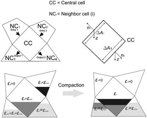
Thus, the common method for bed compaction is considering the particle shrinkage in the bed while bed porosity remains constant [61,69,96,97]. The differences caused by the consumption and transport processes [98] can not be represented by this method. A shrinkage model which simultaneously produced bed shrinkage and porosity raise is also presented for a char bed [63]. In this model the bed collapsed when the threshold porosity was reached, and bed porosity is readjusted over a certain distance within a column. To study the channeling in a grate this model was recently applied to a wood bed [66]. The first model of local solid fraction consumption with varied porosity is presented by Collazo et al. [65]. Unfortunately, no contraction was produced and the bed size stayed almost constant. Following these works, Gomez et al. [79] have recently presented a complete 3-D modeling technique to simulate the transient combustion of packed bed biomass which also produces a continuous bed movement during solid consumption. This method works on energy and mass transfer between cells with mass grouping, by emptying the upper cells and filling the lower cells. Around a central cell, mass and energy are calculated between neighbor cells no matter which cell collapses. A loop over all cells changes every cell conditions are fulfilled. Figure 11.6 shows a schematic of the cells during compaction movement.
In a most recent work, Mehrabian et al. [81] developed a transient 3-D model where a validated comprehensive single particle model [90] for thermally thick biomass particle combustion is applied. Smooth shrinkage of the bed, as well as bed collapse due to uneven consumption of fuel, is taken into account. This model computes the bed shrinkage based on the shrinkage of individual particles. To calculate the new position of particles user-defined function is used. Particles are assumed to be always in contact with the particles beneath and move only in the direction of gravity. A looping procedure is applied to find the particle beneath. Particle positions are updated after each execution of the model so at the end of the time step all particles in the packed bed arrange a compacted bed. Discontinuous shrinkage (bed collapse) and cavities occur in the packed bed due to uneven fuel consumption. Bed porosity is calculated at every time step, which is used to calculate the gas phase pressure drop in the packed bed.
Gas phase modeling: The gas phase conservation equations are continuity, momentum, energy, turbulence, chemical species, and soot. Most authors used the built-in algorithm of the commercial CFD software to solve these equations [76,79,81,99]. The standard k-epsilon model is used to account for the effect of turbulence with enhanced wall treatment. For homogeneous reactions, a finite-rate Eddy dissipation model is used which computes both the Arrhenius rate and Eddy dissipation rate and uses the lower one.
The effect of the porosity on the gas flow was introduced as a source (Eq. 11.30) in the momentum equation [100].
(11.30)
where, coefficients of permeability,
(11.31)
 (11.31)
(11.32)
(11.33)
(11.34)
Heat transfer modeling: Heat and mass transfer plays an important part in the combustion process. Heat and mass transfer is modeled for the solid phase and the interactions of the solid with the gas phase. To model the heat and mass exchanges between phases, many authors have used the famous Wakao and Kaguei correlations for the calculation of Nusselt and Sherwood dimensionless numbers shown in Eqs (11.35) and (11.36), respectively.
(11.35)
(11.36)
These dimensionless numbers are used to calculate the convective heat transfer coefficient (h) and the mass transfer coefficient (km) as follows.
(11.37)
Here, radiation heat transfer has been modeled by a discrete ordinates model (DOM). Gomez et al. [79] modified the standard DOM to calculate the difference in temperature between the solid and the gas phases and high absorptivity of the medium. Mehrabian et al. [81] have also calculated the radiative heat transfer between the particles.
Modeling of packed bed combustion is a comparatively new research area and researchers are still in the very early stages of investigation. The solid conversion mechanism has made this process complex and much effort is needed to overcome the problems of modeling. A complete solid-phase model, bed shrinkage model, modified heat transfer, and radiation model are necessary for further development of the process. Investigation is needed to mitigate the major issues limiting the application of packed bed combustion.
11.6 Modeling of Slagging in Combustion
11.6.1 Fundamentals of Slagging
Coal contains various inorganic contents, such as SiO2, TiO2, Al2O3, CaO, MgO, Na2O, K2O, P2O5, Mn3O4, SO3, Fe2O3, etc. During combustion of coal in power plants, these mineral contents are deposited as slag. Slagging is a process of combustion in which the ash component is heated, becomes molten, and thus is deposited along the furnace refractory wall. This molten ash forms a layer called slag. The advantage of slagging is a reduction in the disposing of unused mineral content in the environment, improved energy efficiency, and broader fuel flexibility. The deposited slag layer also works as a coating which prevents heat loss in the gasifiers. But slagging reduces the overall efficiency of the furnace; excessive slagging reduces reliability and safety because of corrosion. In order to maintain an optimum condition of slagging, a detailed fundamental of slagging is important. For designing and optimization of slagging in a combustor, it is imperative to investigate the related process occurring inside the furnace. In the last decade, research has been concentrated in the effects of oxy-fuel combustion by CFD. Limited attempts have also been taken to investigate the slagging issue. It is very important to know the amount and location of the slag as well as its dynamics. It is not possible to investigate the problems on site unobtrusively and without reasonable effort. The answer is numerical simulation which leads to slagging modeling. In recent years, a number of attempts have been made to utilize CFD methods to model the ash formation and transport process in a pulverized-fuel combustion system. Computational modeling is a way to investigate the performance of slagging for better understanding of this process. Modeling may provide detailed investigations overcoming experimental limitations.
11.6.2 Processes Involved in Slagging
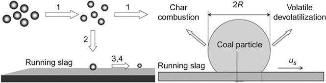
In general, the modeling of slagging consists of several complexes and simultaneous processes, such as the slag flow, particle capture, and particle consumption modeling. Proper understanding and fundamentals in modeling of slagging are important. A graphical representation of the process involved in slag formation is given in Figure 11.7. When the fuel particle hits the wall of the furnace, some of the particles are captured and some of the particles are rebounded from the wall. The captured particles pass through a wall burning process [102]. As input conditions for the slag model, the heat fluxes, slag mass flow rates, and gas temperatures can be integrated from the coupled CFD code.
Char capture modeling: In the coal combustion process, fuel particles are always at the state of melting. It is very difficult for them to drive back to spatial space. Larger particles try to be carried into the gaseous field again after depositing. In coal-fired boilers, the size of most particles is >1 mm, so most of the particles cannot go back to flow space. When these char/ash particles hit the furnace wall, most of the particles are captured on the wall and some particles rebound from the wall. Determining the capturing/rebounding criteria is important in modeling the slagging in CFD. Several authors use a particle capture submodel to define particle-capturing criteria to form slag or not on the refractory wall. Based on the stickiness and the Weber number of the particles, the char capture criteria are summarized in Ref. [103] as shown in Table 11.5. Though a number of capturing criteria are developed, a comprehensive modeling for the ash particle capture is still required.
Table 11.5
Typical char capturing criteria
| Char/ash particle (T-Trap, R-Reflect) | ||||||||
| Temp | Tp>Tcy | Tp<Tcy | ||||||
| Conversion>Cσ | Conversion<Cα | Conversion>Cα | Conversion<Cα | |||||
| We>Weα | We>Weα | We>Weα | We>Weα | We>Weα | We>Weα | We>Weα | We>Weα | |
| Twi<Tcy | T | T | R | T | R | T | R | T |
| Twi<Tcy | R | T | R | T | R | R | R | R |

Wall burning submodels: In slagging furnace, the process of free flow particle combustion, its depositions (trapping/rebounding), and wall burning are simultaneous processes. These processes are interrelated and communicate with each other in terms of physical parameters like viscosity and temperature. The burning characteristics of particles on the molten slag layer with the associated process are presented in Figure 11.7. Fundamentals about the wall burning process are given in Refs [101,104]. After, a char/ash particle is trapped on the refractory wall, it passes through and the wall burning process starts. After sticking on the wall, the molten slag moves in the flow direction. Wall burning is a slower char combustion process because of the slower diffusion of oxygen on the particles’ external surface. To allow for the slower reaction of submerged particles in the wall slag layer, a wall burning sub model is proposed in Refs [102,103,105,106], which considers the sink position of the trapped particles.
11.6.3 Recent Numerical Works
In recent years, emphasis has been given to the furnace slagging problem, as it is considered a threat to the long-term performance of the boiler. Many efforts have been given to identify the problems and related issues to avoid these problems experimentally. Several numerical studies were also carried out to investigate the fundamentals and detailed associated phenomena in these problems.
Table 11.6 shows the summarized endeavors in modeling the formation of slag by researchers. Li et al. [111,114] conducted an experimental study to determine the physical phenomena associated with char–slag transition in an entrained-flow reactor. Seggiani [107] developed a simplified model for the simulation of time-varying slag flow in a Prenflo entrained flow reactor of the IGCC power plant, Spain. Wang et al. [101,104] developed a 1-D steady-state model to determine the deposition and burning characteristics during slagging co-firing of coal and wood. In this model, particle deposition, wall burning, and slag flow are considered. Yong et al. [102,106] developed a steady-state model to describe the flow and heat transfer characteristics in slag layer of solid fuel gasifications by combining the model developed by Seggaini and Wang as described earlier.
Table 11.6
Summary of the modeling attempts for slagging
| Facility | Fuel | Code | Outcome/limitations | References |
| Prenflo gasifier | Coal | This model provides the slag deposit thickness, the temperature across the deposit and heat flux to the metal wall. But this model cannot resolve the slag behavior in the azimuthal direction | [107] | |
| Pilot-scale combustor | Coal and wood | WBSFPCC2 | This model demonstrates the deposition and burning characteristics during slagging co-firing, especially the wall burning mechanisms | [101] |
| Pilot-scale combustor | Coal | WBSFPCC2 | This model considers wall burning subprocess when particle are trapped on slag layer and its effects on the boiler wall performance. This model considers only molten slag thickness; no solid layer thickness is solved | [104] |
| Gasifier | Coal | FLUENT | Developed a multiphase multilayer phase transformation model. The viscosity–temperature relationship in the liquid slag layer is established | [108] |
| 5MWth combustor | Coal | FLUENT | The accumulated molten slag is 1–2 mm, having average slag velocity of 0.1 mm s due to high viscosity | [105] |
| 5MWth combustor | Coal | FLUENT | Ash capturing ratio decreases with the increase in temperature of critical viscosity | [103] |
| 5MWth combustor | Coal | FLUENT | It is found that the wall traps about 56% of the coal particles fed in to the combustor. This model cannot resolve the slag behavior in the azimuthal direction | [102] |
| IGCC Power plant combustor | Coal | GLACIER | This model has been demonstrated for oxygen blown, pressurized system, but for air blown or atmospheric system is not explored | [109] |
| Alumina reactor | Coal | FLUENT | A simple model was suggested for char capture by molten slag surface under high-temperature conditions | [110] |
| A lab-scale LEFR | Coal | FLUENT | Determines particle depositions behavior during char–slag transitions and established a criterion for accurately predicting particle fates | [111] |
| FPTF at ABB | Coal | PCGC-2 | It was observed that heat flux and the deposition rate had a substantial effect on the thermal and physical properties | [112] |
| 512-MW Boiler | Coal | AshProSM | It assesses the combined impact of ash formation and deposition phenomena, fuel quality, ash properties, slagging | [113] |

Bockelie et al. [115] extended the 1-D slag model into the 2-D wall surface in a fuel combustor. Liu and Hao [116] modeled a 2-D slag flow in an entrained flow gasifier using the volume-of-fluid model. Ni et al. [108] used the same technique to model the multiphase multilayer slag flow and phase transformation considering 2-D mesh with uniform ash deposition rate. Chen and Ghoniem [105] developed a comprehensive 3-D slag flow model to determine the slag behavior during coal combustion and gasification in a 5-MW pressurized coal water slurry vertically oriented oxy-fuel furnace. This model fully resolves the 3-D characteristics of char/ash deposition, slag flow, as well as heat transfer through the slag layer. It was observed that molten ash properties are critical to the slag layer buildup.
Figure 11.8 shows the visualization of the molten slag thickness, slag surface flow velocity, slag volume fraction near the wall, respectively, based on Ref. [105]. The result showed that the 1- to 2-mm slag layer is formed on the refractory wall which is basically molten. These molten slags run downward on the refractory wall, gather on the floor of the furnace and exit at the lower wall of the combustor, mostly driven by gravity for the horizontal furnace. The mean slag flow rate is normally about 0.1 mm s−1.

11.7 Example A: Lab-Scale Modeling for Coal Combustion
This numerical work is an attempt to model coal combustion and its related issues and to address the effects of oxy-fuel firing by computational modeling of a small-scale CTF. The main reason for this example is to provide a guideline for designing a new or retrofitting an existing boiler with oxy-fuel combustion capability considering heat transfers. This study will determine the balance between convective and radiative heat transfer for operations of the boiler in air and also in oxy-fuel firing conditions. Overall, this study endeavors to obtain a decent understanding of the mechanism of oxy-fuel coal combustion technique using a finite-volume-based computational tool.
11.7.1 Experimental Study Considered
In order to model the coal combustion, a 0.5-MWth CTF was considered. This facility is equipped for coal combustion under air and oxy-fuel conditions. In the experimental work, studies of the effect of radiative and convective heat transfer and burnout effects of selected coal with different RRs were conducted. The RRs considered in the experimental study were RR 65% (total O2 30.9% and total CO2 69.2% by mass), RR 72% (total O2 25.4% and total CO2 74.6% by mass) and RR 75% (total O2 22.8% and total CO2 77.2% by mass). The definition of RR was given previously. A scaled version of the IFRF aerodynamically air-staged burner with primary oxidizer and coal and secondary preheated oxidizer was used and fired at a constant thermal input of 0.5 MWt for all conditions. The temperatures were maintained at 70°C and 270°C at the primary and secondary inlets, respectively. Constant secondary swirling flow was maintained with the swirled number of 0.6 for all experiments.
11.7.2 Furnace Description and Operating Conditions
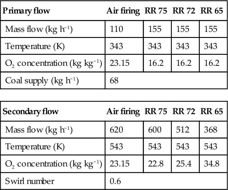
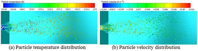
The horizontal furnace consists of a 0.8-m square ceramic-lined wall approximately 4 m long followed by a convergent section leading to a simulated economizer region. The present computational domain has several boundaries such as inlet boundaries including primary oxidizer, secondary oxidizer, coal supply, wall boundaries, and the exit. The inlet boundary conditions of the burner for different combustion cases are given in Table 11.7. Around 80% of the total oxidizers enter the secondary and the rest through the primary. The input power of fuel is 0.5 MWth and the particle mass flow rate is 68 kg h−1 for all cases simulated. Swirled flow was generated in the secondary inlet with prescribed angular velocity in relation to the constant swirl number. To be consistent with the experiments, different walls were kept at different thermal resistances. Considering radiative properties of the wall, the assumed value of emissivity is e=0.85 for the furnace wall. In the present study, used CTF was supplied with pulverized, highly volatile bituminous coal as fuel. The coal is characterized by gross calorific value (GCV) of 27,098 kJ kg−1. Fuel particle distribution is inserted into the computational domain as Rosin Rammler distribution. The particle size range considered in this study is 75–300 µm. The characteristic parameters of Rosin Rammler distribution applied in this study are as follows: maximum particle size, dmax=300 µm, minimum particle size dmin=75 µm, mean size, dRRD, mean=100 µm, and spread, n=5.78. The fuel particle distribution along with the particle temperature distribution and the particle movement in the furnace for the air combustion case are presented in Figure 11.9. From the figure, it is found that the maximum particle temperature achieved in air combustion is around 2250 K.
Table 11.7
The inlet boundary condition for different combustion cases
| Primary flow | Air firing | RR 75 | RR 72 | RR 65 |
| Mass flow (kg h−1) | 110 | 155 | 155 | 155 |
| Temperature (K) | 343 | 343 | 343 | 343 |
| O2 concentration (kg kg−1) | 23.15 | 16.2 | 16.2 | 16.2 |
| Coal supply (kg h−1) | 68 | |||
| Secondary flow | Air firing | RR 75 | RR 72 | RR 65 |
| Mass flow (kg h−1) | 620 | 600 | 512 | 368 |
| Temperature (K) | 543 | 543 | 543 | 543 |
| O2 concentration (kg kg−1) | 23.15 | 22.8 | 25.4 | 34.8 |
| Swirl number | 0.6 | |||
11.7.3 Effect of Different Performance Parameters
Four different combustion environments were investigated in this study. They are: air combustion (23% inlet O2) (case-I) shown as the reference case and three different RFG fuel (oxy-fuel) combustions such as RR 75% (22.8% inlet O2), RR 72% (25.4% inlet O2) and RR 65% (30.9% inlet O2). The feed gases for these combustion environments are summarized in Table 11.7. In all the combustion cases, some variables were always kept constant, such as input power of 0.5 MW, initial conditions (pressure=101,325 Pa, temperature=800 K, ρ=0.67 kg m−3). The mass flow rate of coal was also constant for all the air and oxy-fuel combustion cases. In the experiments, for the oxy-fuel cases, a dry recycle system was simulated where the O2 concentration in the primary transport was maintained at a constant value. A similar condition was maintained in the present numerical analysis.
The velocity vector (m s−1) at the inlet for the air-firing case is shown in Figure 11.10. In order to increase the mixing, stabilize the flame shape and to provide enough time to the oxidizers for complete burning of fuel, the swirled flow is used in the burning systems. The swirl effect is significant in the combustion phenomenon. The primary oxidizer and the coal particles are fed into the furnace through a primary inlet and swirled secondary oxidizers are fed through a secondary air inlet as shown in the burner configuration. The velocity vectors show an internal recirculation zone, reaction zone, and external recirculation zone. The velocity distributions on the axial vertical position at 0.3 m from the burner exit for selected cases are presented in Figure 11.10. From the figure, it is seen that the velocity of oxidizing gas is decreasing from reference case to RR 65% case. This provides more residence time for the fuel particle to stay in the combustion reaction area and thus a better ignition environment which finally improves the flame temperature.
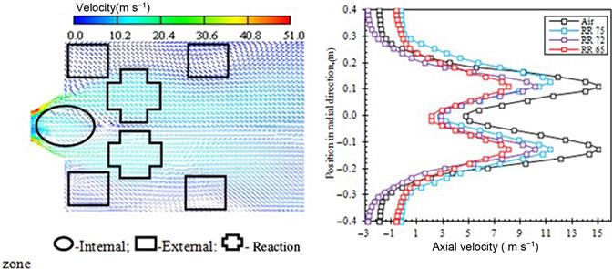
Figure 11.11 shows the temperature distributions for different cases considered. The variation in the flames’ shape between air-fired and RFG fuel-fired cases can be explained on the basis of the differences in the thermodynamics behavior between N2 present in air-firing and CO2 present in oxy-fired cases. The flame temperature for the case of RR 72 is very much similar to that of the air-combustion case. But the flame temperature for RR 75 is slightly lower than the air-fired case. This is due to reduced O2 in RR 75 compared to the air-fired case and availability of CO2 in RR 75. Comparatively more luminous flames are seen in cases RR 75, RR 72, and RR 65. For a lower RR of 65%, much brighter flame is observed compared to the air case. It is clear that the flame temperature increases when oxygen in the inlet is higher and the RFG is less. The flame temperature for the case of RR 65 is higher compared to RR 72 and RR 75.The maximum flame temperatures for air-fired, RR 75, RR 72, and RR 65 were 2250, 2100, 2280, and 2585 K, respectively. This phenomenon may be explained on the basis of the characteristics of turbulent timescale of the EBU combustion model, which suggests a higher flame temperature in the RFG environment with O2-enriched cases due to the quick combustion rate.

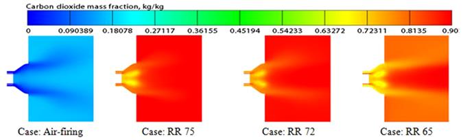
Availability of oxygen (O2) mass fraction (kg kg−1) in the exit of the burner area contributes to the flame characteristics and the ignition environment. The O2 mass fraction (kg kg−1) on a horizontal plane axially along the center of the furnace is shown in Figure 11.12 for different cases. This figure graphically illustrates the O2 mass fraction for the air-fired and three RR cases. It is seen from the figure that the O2 concentration for the air-fired case is similar to that of RR 75 case. Some delay can be observed in the consumption of oxygen (O2) in the air case and RR 75. For RR 72 and RR 65, the profile is more or less similar to the RR 75% case, but the O2 concentration is slightly higher. However, the consumption of O2 is faster and the availability of O2 is much enriched in the case of RR 65% compared to RR 72% and RR 75%, so the ignition condition is improved and better flame is observed just after the exit of the burner. CO2 mass fractions are presented in Figure 11.13 displaying the comparisons of the mass fraction distributions (kg kg−1) of CO2 for all the cases. In the case of air firing, the maximum CO2 concentration in the furnace is 0.193 by mass (kg kg−1). In the case of higher RR, CO2 is much more enriched. But for lower RR 65% cases, this fraction goes down to approximately 0.88 by mass. According to chemical properties [117], CO2 has higher specific heat compared to nitrogen (N2). This property is responsible for absorbing more heat, which protects the furnace wall and controls the overall emissivity. That is why an increase in CO2 in the RR cases has significant importance in the combustion environment compared to the air-fired case. The species mass fraction distribution for different cases at 0.3 m from the burner exit is presented in Figure 11.14.


The predictions of the radiation for all combustion cases in the radiative sections are calculated. The values of radiative heat flux for the RR 75, RR 72, and RR 65 cases are compared against the experimental case. The calculated radiative heat fluxes are in the range of 250–400 kW m−2, whereas for the RR 75, RR 72, and RR 65 cases, the range is 275–340, 270–365, 340–490 kW m−2, respectively. The variation in radiative heat flux with RR can be explained on the basis of an O2-enriched environment. When, the O2 concentration is increased by reducing the RR, the radiative heat flux at the radiative sections increases as the RR is reduced from 75% to 65% by volume at the inlet. When CO2 in the boiler decreases, the Cp of the flue gas decreases and the temperature can be higher, thus resulting in higher radiative heat flux. The predicted radiative heat fluxes for RR 72 and RR 75 are similar to that of the air-firing case. While for 65% RR, comparatively higher radiative heat flux is observed. The comparison of predicted and experimental radiative heat flux is given in Table 11.8.
Table 11.8
Comparison of radiative heat flux (Sir) and carbon-in-ash (CIA, %) measurement
| Case | Carbon in ash (CIA) (%) | Radiative heat flux (KW m−2) | ||
| Experimental | Numerical | Experimental | Numerical | |
| Air firing | 2.10 | 2.45 | 390.00 | 431.58 |
| RR 75% | 0.50 | 1.87 | 340.00 | 393.46 |
| RR 72% | 0.90 | 1.47 | 370.00 | 398.29 |
| RR 65% | 0.50 | 1.45 | 495.00 | 522.71 |

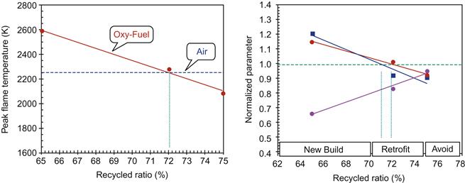
The variation of peak flame temperature for air operation to oxy-fuel operation with different RRs is presented in Figure 11.15. The figure shows that the peak flame temperature for air operation is equivalent to peak oxy-fuel flame temperature at an RR of approximately 72%, which is consistent with experimental results. The normalized radiative and convective heat fluxes for different RR are presented in Figure 11.15. In the case of radiative heat flux, peak values are considered. The graphical presentation shown can help in evaluating a suitable working range for coal combustion under varying RR conditions where both radiative and convective heat transfer can be maintained at a unique balance. This information will help in evaluating the performance of a newly built or an existing retrofitted furnace run on both air and oxy-fuel combustion.
In order to offer direction to the utility power firms to take cost-effective measures by reducing the unburned carbon in fly ash (CIA), it is important to measure the unburned CIA. Also, predicting unburned carbon in fly ash is a significant measure for determining the efficiency of coal combustion in a power plant. CFD modeling offers this opportunity to measure the CIA. One of the objectives of this study was to determine unburned carbon in ash (CIA) for different firing conditions. Table 11.8 compares the numerically calculated CIA percentage with experimental data. CIA at the particles exiting the furnace depends on several factors, such as the particle size distribution, oxygen concentration, and residence time. Numerical results exhibit a similar trend with the experimental ones, for example, improved burnout under oxy-fuel-firing conditions compared to air combustion. This can be attributed to longer residence times for the particles as well as to the higher oxygen concentration in the furnace.
11.8 Example B: Lab-Scale Modeling for Coal/Biomass Co-Firing
The CFD modeling method for oxy-fuel co-combustion of biomass is a significant challenge compared to coal combustion modeling. Only a few CFD attempts at biomass co-combustion in boilers and furnaces are found in literature in either small or large scales. But the detailed mechanism in chemical and thermal reactions and subsequent mechanisms on the influence of irregular-shaped particles are not explored in detail. A few researchers simulated 3-D large-scale tangentially fired power generation plants using CFD [28,45,48,49]. However, there is little study on the modeling of co-firing of coal and biomass under an oxy-fuel combustion environment. The following study determines the effect of co-firing in oxy-fuel combustion of coal and biomass at different co-firing ratios. Overall, this study is an attempt to model the co-firing considering the issues related to design or retrofitting of an existing furnace.
11.8.1 Experimental Study Considered
The data of a CTF considered in this example are a 0.5-MWth lab-scale furnace for coal and biomass combustion under air/oxy-firing condition. The detailed specification and dimensions of the furnace are documented in Ref. [20]. The burner design consists of fuel with a carrier gas supplied through a primary annulus and the swirled combustion air was delivered through a secondary annulus. The swirl is applied in accordance with the experimental setup given in Ref. [20]. In this numerical study, co-combustion was modeled using pulverized coal and biomass as fuel. The coal and biomass are characterized by a GCV of 27.098 and 17.362 MJ kg−1, respectively. The fuel particle sizes were ranged between 75 and 300 µm. For irregular-shaped biomass, around 30% of passing particles must have a maximum size of more than 200 µm. The length-to-diameter ratio for biomass particles is assumed to be 10. The flow rate, temperatures, and oxygen concentrations for different registers vary with the RRs.
11.8.2 Investigated Cases
In this study, different RRs were considered, such as RR 68% (total O2 26.6% and total CO2 73.4% by mass), RR 72% (total O2 23.4% and total CO2 76.6% by mass), and RR 75% (total O2 21.0% and total CO2 79% by mass). The biomass was co-fired with the coal at a mass ratio of 20% and 40% for air-firing and the selected cases of oxy-firing. In all cases, the total mass flow of fuel was maintained to keep the input load of the plant at 0.5 MWth. The fuel mass flow rates into the plant for different co-firing ratios are shown in Table 11.9. One of the main purposes of this study was to investigate the variation of flame temperature, brightness, and luminosity in different combustion environments and to relate the output data in air to oxy-fuel cases for the purposes of retrofitting. Development of a unique balance between convective and radiative heat transfer characteristics is also important.

11.8.3 Outcome of the Investigation
The variations of numerical and experimental data of radiative heat flux in the radiative section of the CTF are studied and presented for all cases in Figure 11.16. The figure shows the radiative heat flux comparison for 20% and 40% biomass sharing in an air-firing case. Overall, a slightly higher range of radiative flux is observed for the 20% case compared to 40%. This is due to the lower amount of moisture and the lower calorific value of the biomass sharing. However, experimental results show an interesting profile for heat flux for 40% biomass sharing in air-firing case. For RRs 68%, 72%, and 75%, the comparison of the radiative heat flux between the numerical and experimental data for 20% and 40% biomass. It can be seen for these cases that as the RR is increased, the radiative heat flux reduces, which can be explained by the O2-enriched environment. When RR is increased by reducing the O2 level, the radiative heat flux is decreased. Comparatively higher and lower radiative heat flux are observed in the case of RR 68 and RR 75, respectively. The volatile content for biomass is higher. It is expected that volatile matter content would proportionately increase flame length and help in easier ignition of coal, leading to an increase in the radiative heat flux in the combustion area. The higher moisture content with the lower calorific value of biomass plays a vital role. With the increase of biomass sharing to 40%, volatile fraction and moisture content increase. The dominant effect of the lower calorific value and higher moisture content of biomass depresses the effect of the volatile content. Thus the principal effect of the lower calorific value and higher moisture content of biomass is to lower the flame temperature, thus creating radiative heat flux. When the share of biomass was increased from 20% to 40%, it was seen that the radiative heat flux was decreased significantly for all cases. This can be explained on the basis of volatile presence. Higher volatile yields of biomass produce more off-gas inside the furnace. This larger volume of off-gas generates a larger flame but lower temperature at a higher biomass share. Higher moisture content and lower calorific value depress the flame temperature canceling the effect of the high volatile content. Due to the lower flame temperature at 40%, radiative heat flux is significantly decreased.

The flame temperature distributions for all the cases are presented in Figure 11.17. The visualization is shown on the vertical plane 0.3 m from the exit of the burner. For all the cases, the biomass fuel burns very close to the burner exit where the peak flame temperature is observed. With the increase in biomass share, the possibility of ignition of fuel within the furnace increases with fuel volatility and since biomass char is more reactive than coal char; this ensures that the biomass burns out early within the furnace. Therefore, the co-combustion flames are larger in volume. Determining the suitable level of highly volatile biomass is important for better efficiency of the furnace. Higher flame temperature during co-firing can be achieved by injecting less biomass. When the biomass share is increased to 40%, a comparatively larger volume of flames is observed. The temperature distribution shows that the addition of biomass to coal results in a decrease in gas temperature in the respective oxy-fuel cases. It can be stated that the rate of combustion decreased with the increase in biomass particle size, leading to lower temperature. Large particles,greater than 200 µm, are more in a higher concentration for 40% compared to 20% biomass shares.

Figure 11.18 represents the relationship between the convective and radiative heat transfer and the flame temperature for (i) 20% share of biomass and (ii) 40% share of biomass. This relationship has been obtained comparing the normalized data of peak flame temperature and peak radiative heat flux and convective heat transfer predicted. This type of representation is useful for the purpose of retrofitting of existing plants, by choosing the proper RR equivalent to air-firing. Defining a working range for different fuel ratio under an oxy-fuel condition is important. This will provide a unique balance between convective and radiative heat transfer and flame temperature formatted inside the furnace run on air and oxy-combustion. The variations of different normalized parameters for a 20% share of biomass are presented in Figure 11.18(a). It is seen in this figure that air equivalent peak flame temperature is found at RR 71%. Similar to that air equivalent peak radiative heat flux is also found at RR 71%. When radiative heat flux decreases with the increase in RR, convective heat flux increases. This is due to the increased convective heat transfer coefficient because of increased mass flow at higher RR. Similar to a 20% share of biomass, the working range for a 40% share of biomass is presented in Figure 11.18(b). The trend is similar to the 20% case, but air equivalent peak flame temperature and peak radiative heat flux are found at 70% RR. From this analysis, it is identified that radiative heat flux and flame temperature are significantly manipulated by RR and the retrofitting option is well justified. Also, with the increase in biomass share, an air equivalent heat flux/flame temperature is found to the lower RR.

In order to reduce the amount of unburned carbon and to improve the efficiency of the plant, determination of unburned CIA is significant. The CIA data are presented in Table 11.10. Comparatively, improved burnout under oxy-fuel-firing conditions is observed compared to air combustion for different biomass share cases. It is evident that with the increase in biomass share, the CIA amount is decreased in most cases. The amount of CIA depends on several factors such as particle size, combustion environment, and residence time. The decrease in overall CIA content for increased biomass share is not only due to improved combustion conditions which favor coal particles but also the contribution of both fuels to the favorable result.

11.9 Conclusion
The combustion of fossil fuels is a thermochemical conversion technology for power generation. In order to understand the technologies that are used for CO2 capture in conventional power plants, it is important to understand the systems of leading technology for these power plants. Among them, oxy-fuel technology is the most significant option considering emissions’ capturing capability. Combustion of biomass, municipal solid waste combustion in a packed bed is also a source of pollutant emissions. Combustion of solid fuel itself is a complex phenomenon because of the compound mechanisms and parameters involved. Slag formation in the combustion equipment is treated as a serious problem. In order to maintain an optimum condition of slagging, a detailed fundamental of the slagging is important. For designing and optimization of slagging combustor, it is imperative to investigate the related processes occurring inside the furnace. It is important to be able to accurately investigate the emissions level, power generation, and slag formation from combustion equipment, especially with the present concerns about GHG emissions. Numerical modeling is an effective way to investigate the performance related to the design and optimization of the problem in combustion. It is not possible to investigate the problems on-site unobtrusively and without reasonable effort. The answer is numerical simulation, which leads to combustion modeling. Overall, this chapter has reviewed recent advances in the carbon capturing and storage systems and related issues, fundamentals of coal/biomass combustion methodology, packed bed combustion modeling, and slag formation modeling concepts. Examples were presented demonstrating the application of the recent developments utilizing CFD methods to model the heat transfer performance, emissions, ash formation, and transport processes in pulverized coal and biomass combustion systems under different combustion environments.
Nomenclature
Ac Pre-exponential factor (s−1)
![]() Cross-sectional area of particle (m2)
Cross-sectional area of particle (m2)
Av Pre-exponential factor (s−1)
![]() Combustion model constant (=3.0)
Combustion model constant (=3.0)
![]() Combustion model constant (=0.5)
Combustion model constant (=0.5)
Dii Diffusivity of the species i in the mixture (m2 s−1)
Dp Diameter of the particle (µm)
Ec Activation energy (kJ mol−1)
Ev Activation energy (kJ mol−1)
G Production due to the buoyancy force
h Convection coefficient (W m−2 K−1)
k Thermal conductivity (W m−1 K−1)
km Mass transfer constant (m s−1)
K Turbulent kinetic energy (m2 s−2)
![]() Rate constant of devolatilization
Rate constant of devolatilization
min Minimum value of the operator
mPFG Amount of product flue gas
mRFG Amount of recycled flue gas
![]() Mass of particles at devolatilization (kg)
Mass of particles at devolatilization (kg)
p Sum of partial pressure (N m−2)
![]() Partial pressure of oxygen at furnace (N m−2)
Partial pressure of oxygen at furnace (N m−2)
![]() Oxygen partial pressure at surface (N m−2)
Oxygen partial pressure at surface (N m−2)
![]() Fuel consumption rate (kg m−3s−1)
Fuel consumption rate (kg m−3s−1)
S Stoichiometric air/fuel ratio
![]() Temperature of the particle (K)
Temperature of the particle (K)
![]() Velocity in the ith direction (m s−1)
Velocity in the ith direction (m s−1)
V Product of volatiles at time (t)
![]() Velocity of the particle (m s−1)
Velocity of the particle (m s−1)
xi Spatial distance in the ith direction
![]() Mass fraction of fuel (kg kg−1)
Mass fraction of fuel (kg kg−1)
![]() Mass fraction of product (kg kg−1)
Mass fraction of product (kg kg−1)
![]() Mass fraction of oxidizer (kg kg−1)
Mass fraction of oxidizer (kg kg−1)
Greek Symbols
![]() Generation or consumption velocities
Generation or consumption velocities
λ Thermal conductivity (W mK−1)
![]() Total radiation intensity (W m−2)
Total radiation intensity (W m−2)
![]() Turbulent dissipation rate (m2 s−3)
Turbulent dissipation rate (m2 s−3)
![]() Density at particle phase (kg m−3)
Density at particle phase (kg m−3)
List of Abbreviations
AASB Aerodynamically air-staged burner
DTRM Discrete transfer radiation method
EBU Eddy breakup combustion model