15

From NLP to Task-Agnostic Transformer Models

Up to now, we have examined variations of the original Transformer model with encoder and decoder layers, and we explored other models with encoder-only or decoder-only stacks of layers. Also, the size of the layers and parameters has increased. However, the fundamental architecture of the transformer retains its original structure with identical layers and the parallelization of the computing of the attention heads.

In this chapter, we will explore innovative transformer models that respect the basic structure of the original Transformer but make some significant changes. Scores of transformer models will appear, like the many possibilities a box of LEGO^© pieces gives. You can assemble those pieces in hundreds of ways! Transformer model sublayers and layers are the LEGO^© pieces of advanced AI.

We will begin by asking which transformer model to choose among the many offers and the ecosystem we will implement them in.

Then we will discover Locality Sensitivity Hashing (LSH) buckets and chunking in Reformer models. We will then learn what disentanglement is in DeBERTa models. DeBERTa also introduces an alternative way of managing positions in the decoder. DeBERTA’s high-powered transformer model exceeds human baselines.

Our last step stops will be to discover powerful computer vision transformers such as Vit, CLIP, and DALL-E. We can add CLIP and DALL-E to OpenAI GPT-3 and Google BERT (trained by Google) to the very small group of foundation models.

These powerful foundation models prove that transformers are task-agnostic. A transformer learns sequences. These sequences include vision, sound, and any type of data represented as a sequence.

Images contain sequences of data-like language. We will run ViT, CLIP, and DALL-E models to learn. We will take vision models to innovative levels.

By the end of the chapter, you will see that the world of task-agnostic transformers has evolved into a universe of imagination and creativity.

This chapter covers the following topics:

• Choosing a transformer model
• The Reformer transformer model
• Locality Sensitivity Hashing (LSH)
• Bucket and chunking techniques
• The DeBERTA transformer model
• Disentangled attention
• Absolute positions
• Text-image vision transformers with CLIP
• DALL-E, a creative text-image vision transformer

Our first step will be to see how to choose a model and an ecosystem.

Choosing a model and an ecosystem

We thought that testing transformer models by downloading them would require machine and human resources. Also, you might have thought that if a platform doesn’t have an online sandbox by this time, it will be a risk to go further because of the work to test a few examples.

However, sites such as Hugging Face download pretrained models automatically in real time, as we will see in The Reformer and DeBERTa sections! So, what should we do? Thanks to that, we can run Hugging Face models in Google Colab without installing anything on the machine ourselves. We can also test Hugging Face models online.

The idea is to analyze without having anything to “install.” “Nothing to Install” in 2022 can mean:

• Running a transformer task online
• Running a transformer on a preinstalled Google Colaboratory VM that seamlessly downloads a pretrained model for a task, which we can run in a few lines
• Running a transformer through an API

The definition of “install” has expanded over the past few years. The definition of “online” has widened. We can consider using a few lines of code to run an API as a meta-online test.

We will refer to “without installing,” and “online” in a broad sense in this section. Figure 15.1 shows how we should test models “online”:

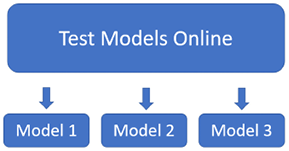
Figure 15.1: Testing transformer models online

Testing in this decade has become flexible and productive, as the following shows:

• Hugging Face hosts API models such as DeBERTa and some other models. In addition, Hugging Face offers an AutoML service to train and deploy transformer models in their ecosystem.
• OpenAI’s GPT-3 engine runs on the online playground and provides an API. OpenAI offers models that cover many NLP tasks. The models require no training. GPT-3’s billion-parameter zero-shot engine is impressive. It shows that transformer models with many parameters produce better results overall. Microsoft Azure, Google Cloud AI, AllenNLP, and other platforms offer interesting services.
• An online model analysis can be done by reading a paper if it is worthwhile. A good example is Google’s publication by Fedus et al., (2021), on Switch Transformers: Scaling to Trillion Parameter Models with Simple and Efficient Sparsity. Google increased the size of the T5-based models we studied in Chapter 8, Applying Transformers to Legal and Financial Documents for AI Text Summarization. This paper confirms the strategy of large online models such as GTP-3.

However, in the end, you are the one taking the risk of choosing one solution over another. The time you spend on exploring platforms and models will help you optimize the implementation of your project once you have made your choice.

You can host your choice in three different ways, as shown in Figure 15.2:

• On a local machine using an API. OpenAI, Google Cloud AI, Microsoft Azure AI, Hugging Face, and others provide good APIs. An application can be on a local machine and not on a cloud platform but can go through a cloud service with an API.
• On a cloud platform such as Amazon Web Services (AWS) or Google Cloud. You can train, fine-tune, test, and run the models on these platforms. In this case, there is no application on a local machine. Everything is on the cloud.
• From anywhere using an API! On a local machine, a data center VM, or from anywhere. This means that the API would be integrated in a physical system such as a windmill, an airplane, a rocket, or an autonomous vehicle. The system could thus permanently connect with another system through an API.

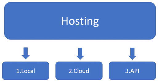
Figure 15.2: Implementing options for your models

In the end, it is up to you to make the decision. Take your time. Test, analyze, compute the costs, and work as a team to listen to different perspectives. The more you understand how transformers work, the better the choices you make will be.

Let’s now explore the Reformer, a variation of the original Transformer model.

The Reformer

Kitaev et al. (2020) designed the Reformer to solve the attention and memory issues, adding functionality to the original Transformer model.

The Reformer first solves the attention issue with Locality Sensitivity Hashing (LSH) buckets and chunking.

LSH searches for nearest neighbors in datasets. The hash function determines that if datapoint q is close to p, then hash(q) == hash(p). In this case, the data points are the keys of the transformer model’s heads.

The LSH function converts the keys into LSH buckets (B1 to B4 in Figure 15.3) in a process called LSH bucketing, just like how we would take objects similar to each other and put them in the same sorted buckets.

The sorted buckets are split into chunks (C1 to C4 in Figure 15.3) to parallelize. Finally, attention will only be applied within the same bucket in its chunk and the previous chunk:

Figure 15.3: LSH attention heads

LSH bucketing and chunking considerably reduce the complexity from O(L²), attending to all the word pairs, to O(LlogL), only attending to the content of each bucket.

The Reformer also solves the memory issue of recomputing each layer’s input instead of storing the information for multi-layer models. The recomputing is achieved on-demand instead of consuming terabytes of memory for some large multi-layer models.

We will now use a Reformer model trained on the English translation of Crime and Punishment by Fyodor Dostoevsky.

Running an example

Let’s run it directly online with the hosted inference API. The input sentence is:

The student was impoverished and did not know what to do.

The link to the online interface contains the input:

https://huggingface.co/google/reformer-crime-and-punishment?text=The+student+was+impoverished+and+did+not+know+what+to+do

The hosted inference API appears with the input sentence. Click on compute to obtain an inference, and the result will appear right under the input:

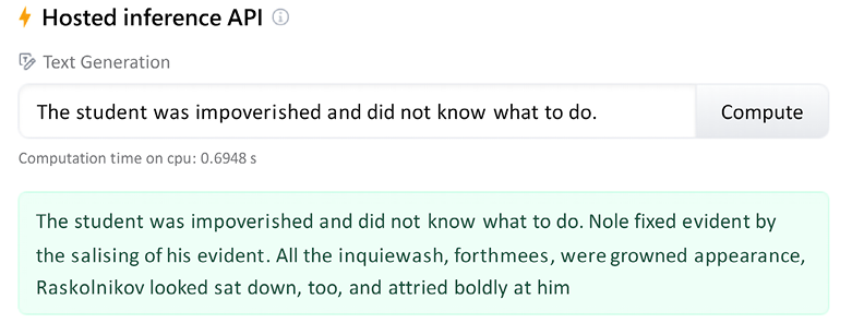
Figure 15.4: The Reformer’s hosted inference API

You might get a different response since the algorithm is stochastic. The Reformer was reasonably trained, though not with a supercomputer with billions of bits of information like OpenAI’s GPT-3. The result of the Reformer is not very impressive. It would take more training and fine-tuning to obtain better results.

OpenAI’s GPT-3 engine produces the following result for text completion:

The student was impoverished and did not know what to do. He did not have any one to turn to and could not find a place to stay. He took out a pad from his bag and started writing. He wrote:

"My name is XXXXXXXXXX. I am a student at XXXXXXXXXX. I have no family, no friends, no money."

The result is more convincing. You can access OpenAI’s playground after having signed up: https://openai.com/

This shows that a highly well-trained transformer model containing billions of parameters can outperform an innovative transformer model architecture.

Will supercomputer-driven cloud AI platforms progressively outperform local attempts or even less powerful cloud platforms? You need to address these issues through prototypes before investing in one solution over another.

DeBERTa introduces another innovative architecture, which we will now explore.

DeBERTa

Another new approach to transformers can be found through disentanglement. Disentanglement in AI allows you to separate the representation features to make the training process more flexible. Pengcheng He, Xiaodong Liu, Jianfeng Gao, and Weizhu Chen designed DeBERTa, a disentangled version of a transformer, and described the model in an interesting article: DeBERTa: Decoding-enhanced BERT with Disentangled Attention: https://arxiv.org/abs/2006.03654

The two main ideas implemented in DeBERTa are:

• Disentangle the content and position in the transformer model to train the two vectors separately
• Use an absolute position in the decoder to predict masked tokens in the pretraining process

The authors provide the code on GitHub: https://github.com/microsoft/DeBERTa

DeBERTa exceeds the human baseline on the SuperGLUE leaderboard:

Figure 15.5: DeBERTa on the SuperGLUE leaderboard

Let’s run an example on Hugging Face’s cloud platform.

Running an example

To run an example on Hugging Face’s cloud platform, click on the following link:

https://huggingface.co/cross-encoder/nli-deberta-base

The hosted inference API will appear with an example and output of possible class names:

Figure 15.6: DeBERTa’s hosted inference API

The possible class names are mobile, website, billing, and account access.

The result is interesting. Let’s compare it to a GPT-3 keyword task. First, sign up on https://openai.com/

Enter Text as the input and Keywords to ask the engine to find keywords:

Text: Last week I upgraded my iOS version and ever since then my phone has been overheating whenever I use your app.

Keywords: app, overheating, phone

The possible keywords are app, overheating, and phone.

We have gone through the DeBERTa and GPT-3 transformers. We will now extend transformers to vision models.

From Task-Agnostic Models to Vision Transformers

Foundation models, as we saw in Chapter 1, What Are Transformers?, have two distinct and unique properties:

• Emergence – Transformer models that qualify as foundation models can perform tasks they were not trained for. They are large models trained on supercomputers. They are not trained to learn specific tasks like many other models. Foundation models learn how to understand sequences.
• Homogenization – The same model can be used across many domains with the same fundamental architecture. Foundation models can learn new skills through data faster and better than any other model.

GPT-3 and Google BERT (only the BERT models trained by Google) are task-agnostic foundation models. These task-agnostic models lead directly to ViT, CLIP, and DALL-E models. Transformers have uncanny sequence analysis abilities.

The level of abstraction of transformer models leads to multi-modal neurons:

• Multi-modal neurons can process images that can be tokenized as pixels or image patches. Then they can be processed as words in vision transformers. Once an image has been encoded, transformer models see the tokens as any word token, as shown in Figure 15.7:

  

  Figure 15.7: Images can be encoded into word-like tokens

In this section, we will go through:

• ViT, vision transformers that process images as patches of words
• CLIP, vision transformers that encode text and image
• DALL-E, vision transformers that construct images with text

Let’s begin by exploring ViT, a vision transformer that processes images as patches of words.

ViT – Vision Transformers

Dosovitskiy et al. (2021) summed up the essence of the vision transformer architecture they designed in the title of their paper: An Image is Worth 16x16 Words: Transformers for Image Recognition at Scale.

An image can be converted into patches of 16x16 words.

Let’s first see the architecture of a ViT before looking into the code.

The Basic Architecture of ViT

A vision transformer can process an image as patches of words. In this section, we will go through the process in three steps:

1. Splitting the image into patches
2. A linear projection of the patches
3. The hybrid input embedding sublayer

The first step is to SPLIT the image into equal-sized patches.

Step 1: Splitting the image into patches

The image is split into n patches, as shown in Figure 15.8. There is no rule saying how many patches as long as all the patches have the same dimensions, such as 16x16:

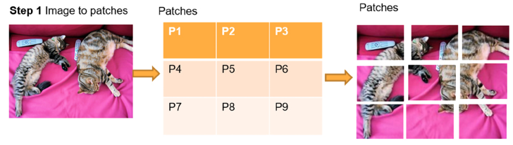
Figure 15.8: Splitting an image into patches

The patches of equal dimensions now represent the words of our sequence. The problem of what to do with these patches remains. We will see that each type of vision transformer has its own method.

In this case, for the ViT, Step 2 will be to make a linear projection of flattened images.

Step 2: Linear projection of flattened images

Step 1 converted an image to equal-sized patches. The motivation of the patches is to avoid processing the image pixel by pixel. However, the problem remains to find a way to process the patches.

The team at Google Research decided to design a linear projection of flattened images with the patches obtained by splitting the image, as shown in Figure 15.9:

Figure 15.9: Linear projection of flattened images

The idea is to obtain a sequence of work-like patches. The remaining problem is to embed the sequence of flattened images.

Step 3: The hybrid input embedding sublayer

Word-like image sequences can fit into a transformer. The problem is that they still are images!

Google Research decided that a hybrid input model would do the job, as shown in Figure 15.10:

• Add a convolutional network to embed the linear projection of the patches
• Add positional encoding to retain the structure of the original image
• Then process the embedded input with a standard original BERT-like encoder

Figure 15.10: A hybrid input sublayer and a standard encoder

Google Research found a clever way to convert an NLP transformer model into a vision transformer.

Now, let’s implement a Hugging Face example of a vision transformer in code.

Vision transformers in code

In this section, we will focus on the main areas of code that relate to the specific architecture of vision transformers.

Open Vision_Transformers.ipynb, which is in the GitHub repository for this chapter.

Google Colab VM’s contain many pre-installed packages such as torch and torchvision. You can display them by uncommenting the command in the first cell of the notebook:

#Uncomment the following command to display the list of pre-installed modules 
#!pip list -v  

Then go to the Vision Transformer (ViT) cell of the notebook. The notebook first installs Hugging Face transformers and imports the necessary modules:

!pip install transformers
from transformers import ViTFeatureExtractor, ViTForImageClassification
from PIL import Image
import requests

We then download an image from the COCO dataset. You can find a comprehensive corpus of datasets on their website if you wish to experiment further: https://cocodataset.org/

Let’s download from the VAL2017 dataset. Follow the COCO dataset website instructions to obtain these images through programs or download the datasets locally.

The VAL2017 contains 5,000 images we can choose from to test this ViT model. You can run any of the 5,000 images.

Let’s test the notebook with the image of the cats. We first retrieve the image of the cats through their URL:

url = 'http://images.cocodataset.org/val2017/000000039769.jpg'
image = Image.open(requests.get(url, stream=True).raw)

We next download Google’s feature extractor and classification model:

feature_extractor = ViTFeatureExtractor.from_pretrained('google/vit-base-patch16-224')
model = ViTForImageClassification.from_pretrained('google/vit-base-patch16-224')

The model was trained on 224 x 244 resolution images but was presented with 16 x 16 patches for feature extraction and classification. The notebook runs the model and makes a prediction:

inputs = feature_extractor(images=image, return_tensors="pt")
outputs = model(**inputs)
logits = outputs.logits
# model predicts one of the 1000 ImageNet classes
predicted_class_idx = logits.argmax(-1).item()
print("Predicted class:",predicted_class_idx,": ", model.config.id2label[predicted_class_idx])

The output is:

Predicted class: 285 :  Egyptian cat

Explore the code that follows the prediction, which gives us information at a low level, among which are:

• model.config.id2label, which will list the labels of the classes. The 1000 label classes explain why we obtain a class and not a detailed text description:

  {0: 'tench, Tinca tinca',1: 'goldfish, Carassius auratus', 2: 'great white shark, white shark, man-eater, man-eating shark, Carcharodon carcharias',3: 'tiger shark, Galeocerdo cuvieri',...,999: 'toilet tissue, toilet paper, bathroom tissue'}
  
• model, which will display the architecture of the model that begins with the hybrid usage of a convolutional input sublayer:

  (embeddings): ViTEmbeddings(
    (patch_embeddings): PatchEmbeddings(
      (projection): Conv2d(3, 768, kernel_size=(16, 16), stride=(16, 16))
    )
  

After the convolutional input embedding sublayer, the model is a BERT-like encoder.

Take your time to explore this innovative move from NLP transformers to transformers for images, leading to transformers for everything quite rapidly.

Now, let’s go through CLIP, another computer vision model.

CLIP

Contrastive Language-Image Pre-Training (CLIP) follows the philosophy of transformers. It plugs sequences of data in its transformer-type layers. Instead of sending text pairs, this time, the model sends text-image pairs. Once the data is tokenized, encoded, and embedded, CLIP, a task-agnostic model, learns text-image pairs as with any other sequence of data.

The method is contrastive because it looks for the contrasts in the features of the image. It is the method we use in some magazine games in which we have to find the differences, the contrasts, between two images.

Let’s first see the architecture of CLIP before looking into the code.

The Basic Architecture of CLIP

Contrastive: the images are trained to learn how they fit together through their differences and similarities. The image and captions find their way toward each other through (joint text, image) pretraining. After pretraining, CLIP learns new tasks.

CLIPs are transferable because they can learn new visual concepts, like GPT models, such as action recognition in video sequences. The captions lead to endless applications.

ViT splits images into word-like patches. CLIP jointly trains text and image encoders for (caption, image) pairs to maximize cosine similarity, as shown in Figure 15.11:

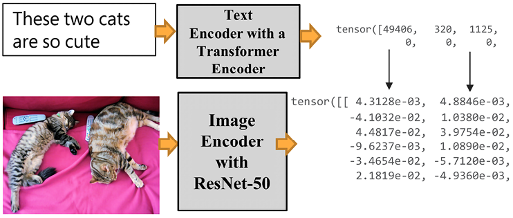
Figure 15.11: Jointly training text and images

Figure 15.11 shows how the transformer will run a standard transformer encoder for the text input. It will run a ResNet 50-layer CNN for the images in a transformer structure. ResNet 50 was modified to run an average pooling layer in an attention pooling mechanism with a multi-head QKV attention head.

Let’s see how CLIP learns text-image sequences to make predictions.

CLIP in code

Open Vision_Transformers.ipynb, which is in the repository for this chapter on GitHub. Then go to the CLIP cell of the notebook.

The program begins by installing PyTorch and CLIP:

!pip install ftfy regex tqdm
!pip install git+https://github.com/openai/CLIP.git

The program also imports the modules and CIFAR-100 to access the images:

import os
import clip
import torch
from torchvision.datasets import CIFAR100

There are 10,000 images available with an index between 0 and 9,999. The next step is to select an image we want to run a prediction on:

Figure 15.12: Selecting an image index

The program then loads the model on the device that is available (GPU or CPU):

# Load the model
device = "cuda" if torch.cuda.is_available() else "cpu"
model, preprocess = clip.load('ViT-B/32', device)

The images are downloaded:

# Download the dataset
cifar100 = CIFAR100(root=os.path.expanduser("~/.cache"), download=True, train=False)

The input is prepared:

# Prepare the inputs
image, class_id = cifar100[index]
image_input = preprocess(image).unsqueeze(0).to(device)
text_inputs = torch.cat([clip.tokenize(f"a photo of a {c}") for c in cifar100.classes]).to(device)

Let’s visualize the input we selected before running the prediction:

import matplotlib.pyplot as plt
from torchvision import transforms
plt.imshow(image)

The output shows that index 15 is a lion:

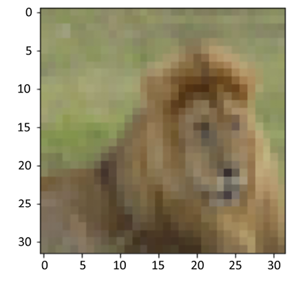
Figure 15.13: Image of Index 15

We know this is a lion because we are humans. A transformer initially designed for NLP has to learn what an image is. We will now see how well it can recognize images.

The program shows that it is running a joint transformer model by separating the image input from the text input when calculating the features:

# Calculate features
with torch.no_grad():
    image_features = model.encode_image(image_input)
    text_features = model.encode_text(text_inputs)

Now CLIP makes a prediction and displays the top five predictions:

# Pick the top 5 most similar labels for the image
image_features /= image_features.norm(dim=-1, keepdim=True)
text_features /= text_features.norm(dim=-1, keepdim=True)
similarity = (100.0 * image_features @ text_features.T).softmax(dim=-1)
values, indices = similarity[0].topk(5)
# Print the result
print("
Top predictions:
")
for value, index in zip(values, indices):
    print(f"{cifar100.classes[index]:>16s}: {100 * value.item():.2f}%")

You can modify topk(5) if you want to obtain more or fewer predictions. The top five predictions are displayed:

Top predictions:
            lion: 96.34%
           tiger: 1.04%
           camel: 0.28%
      lawn_mower: 0.26%
         leopard: 0.26%

CLIP found the lion, which shows the flexibility of transformer architectures.

The next cell displays the classes:

cifar100.classes

You can go through the classes to see that with only one label per class, which is restrictive, CLIP did a good job:

[...,'kangaroo','keyboard','lamp','lawn_mower','leopard','lion',
 'lizard', ...]

The notebook contains several other cells describing the architecture and configuration of CLIP that you can explore.

The model cell is particularly interesting because you can see the visual encoder that begins with a convolutional embedding like for the ViT model and then continues as a “standard” size-768 transformer with multi-head attention:

CLIP(
  (visual): VisionTransformer(
    (conv1): Conv2d(3, 768, kernel_size=(32, 32), stride=(32, 32), bias=False)
    (ln_pre): LayerNorm((768,), eps=1e-05, elementwise_affine=True)
    (transformer): Transformer(
      (resblocks): Sequential(
        (0): ResidualAttentionBlock(
          (attn): MultiheadAttention(
            (out_proj): NonDynamicallyQuantizableLinear(in_features=768, out_features=768, bias=True)
          )
          (ln_1): LayerNorm((768,), eps=1e-05, elementwise_affine=True)
          (mlp): Sequential(
            (c_fc): Linear(in_features=768, out_features=3072, bias=True)
            (gelu): QuickGELU()
            (c_proj): Linear(in_features=3072, out_features=768, bias=True)
          )
          (ln_2): LayerNorm((768,), eps=1e-05, elementwise_affine=True)
        )

Another interesting aspect of the model cell is to look into the size-512 text encoder that runs jointly with the image encoder:

(transformer): Transformer(
    (resblocks): Sequential(
      (0): ResidualAttentionBlock(
        (attn): MultiheadAttention(
          (out_proj): NonDynamicallyQuantizableLinear(in_features=512, out_features=512, bias=True)
        )
        (ln_1): LayerNorm((512,), eps=1e-05, elementwise_affine=True)
        (mlp): Sequential(
          (c_fc): Linear(in_features=512, out_features=2048, bias=True)
          (gelu): QuickGELU()
          (c_proj): Linear(in_features=2048, out_features=512, bias=True)
        )
        (ln_2): LayerNorm((512,), eps=1e-05, elementwise_affine=True)
      )

Go through the cells that describe the architecture, configuration, and parameters to see how CLIP represents data.

We showed that task-agnostic transformer models process image-text pairs as text-text pairs. We could apply task-agnostic models to music-text, sound-text, music-images, and any type of data pairs.

We will now explore DALL-E, another task-agnostic transformer model that can process images and text.

DALL-E

DALL-E, as with CLIP, is a task-agnostic model. CLIP processed text-image pairs. DALL-E processes the text and image tokens differently. DALL-E’s input is a single stream of text and image of 1,280 tokens. 256 tokens are for the text, and 1,024 tokens are used for the image. DALL-E is a foundation model like CLIP.

DALL-E was named after Salvador Dali and Pixar’s WALL-E. The usage of DALL-E is to enter a text prompt and produce an image. However, DALL-E must first learn how to generate images with text.

DALL-E is a 12-billion-parameter version of GPT-3.

This transformer generates images from text descriptions using a dataset of text-image pairs.

The Basic Architecture of DALL-E

Unlike CLIP, DALL-E concatenates up to 256 BPE-encoded text tokens with 32×32 = 1,024 image tokens, as shown in Figure 15.14:

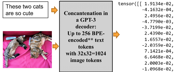
Figure 15.14: DALL-E concatenates text and image input

Figure 15.14 shows that this time, our cat image is concatenated with the input text.

DALL-E has an encoder and a decoder stack, which is built with a hybrid architecture of infusing convolutional functions in a transformer model.

Let’s peek into the code to see how the model works.

DALL-E in code

In this section, we will see how DALL-E reconstructs images.

Open Vision_Transformers.ipynb. Then go to the DALL-E cell of the notebook. The notebook first installs OpenAI DALL-E:

!pip install DALL-E

The notebook downloads the images and processes an image:

import io
import os, sys
import requests
import PIL
import torch
import torchvision.transforms as T
import torchvision.transforms.functional as TF
from dall_e import map_pixels, unmap_pixels, load_model
from IPython.display import display, display_markdown
target_image_size = 256
def download_image(url):
    resp = requests.get(url)
    resp.raise_for_status()
    return PIL.Image.open(io.BytesIO(resp.content))
def preprocess(img):
    s = min(img.size)
    
    if s < target_image_size:
        raise ValueError(f'min dim for image {s} < {target_image_size}')
        
    r = target_image_size / s
    s = (round(r * img.size[1]), round(r * img.size[0]))
    img = TF.resize(img, s, interpolation=PIL.Image.LANCZOS)
    img = TF.center_crop(img, output_size=2 * [target_image_size])
    img = torch.unsqueeze(T.ToTensor()(img), 0)
    return map_pixels(img)

The program now loads the OpenAI DALL-E encoder and decoder:

# This can be changed to a GPU, e.g. 'cuda:0'.
dev = torch.device('cpu')
# For faster load times, download these files locally and use the local paths instead.
enc = load_model("https://cdn.openai.com/dall-e/encoder.pkl", dev)
dec = load_model("https://cdn.openai.com/dall-e/decoder.pkl", dev)

I added the enc and dec cells so that you can look into the encoder and decoder blocks to see how this hybrid model works: the convolutional functionality in a transformer model and the concatenation of text and image input.

The image processed in this section is mycat.jpg (creator: Denis Rothman, all rights reserved, written permission required to reproduce it). The image is in the Chapter15 directory of this book’s repository. It is downloaded and processed:

x=preprocess(download_image('https://github.com/Denis2054/AI_Educational/blob/master/mycat.jpg?raw=true'))

Finally, we display the original image:

display_markdown('Original image:')
display(T.ToPILImage(mode='RGB')(x[0]))

The output displays the image:

Figure 15.15: An image of a cat

Now, the program processes and displays the reconstructed image:

import torch.nn.functional as F
z_logits = enc(x)
z = torch.argmax(z_logits, axis=1)
z = F.one_hot(z, num_classes=enc.vocab_size).permute(0, 3, 1, 2).float()
x_stats = dec(z).float()
x_rec = unmap_pixels(torch.sigmoid(x_stats[:, :3]))
x_rec = T.ToPILImage(mode='RGB')(x_rec[0])
display_markdown('Reconstructed image:')
display(x_rec)

The reconstructed image looks extremely similar to the original:

Figure 15.16: DALL-E reconstructs the image of the cat

The result is impressive. DALL-E learned how to generate images on its own.

The full DALL-E source code is not available at the time of the book’s writing and might never be. An OpenAI API to generate images from text prompts is not online yet. But keep your eyes open!

In the meantime, we can continue discovering DALL-E on OpenAI at https://openai.com/blog/dall-e/

Once you have reached the page, scroll down to the examples provided. For example, I chose a photo of Alamo Square in San Francisco as a prompt:

Figure 15.17: Prompt for Alamo Square, SF

Then I modified “at night” to “in the morning”:

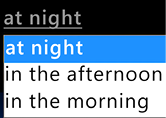
Figure 15.18: Modifying the prompt

DALL-E then generated a multitude of text2image images:

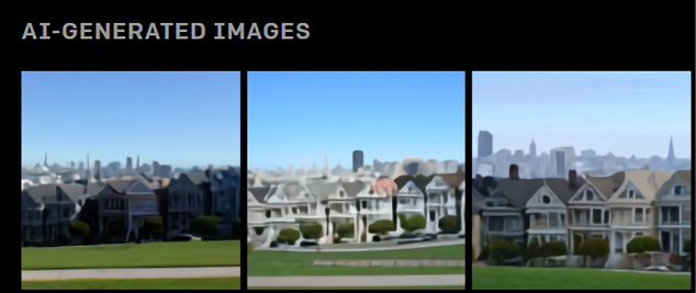
Figure 15.19: Generating images from text prompts

We have implemented ViT, CLIP, and DALL-E, three vision transformers. Let’s go through some final thoughts before we finish.

An expanding universe of models

New transformer models, like new smartphones, emerge nearly every week. Some of these models are both mind-blowing and challenging for a project manager:

• ERNIE is a continual pretraining framework that produces impressive results for language understanding.

  Paper: https://arxiv.org/abs/1907.12412

  Challenges: Hugging Face provides a model. Is it a full-blown model? Is it the one Baidu trained to exceed human baselines on the SuperGLUE Leaderboard (December 2021): https://super.gluebenchmark.com/leaderboard? Do we have access to the best one or just a toy model? What is the purpose of running AutoML on such small versions of models? Will we gain access to it on the Baidu platform or a similar one? How much will it cost?

• SWITCH: A trillion-parameter model optimized with sparse modeling.

  Paper: https://arxiv.org/abs/2101.03961

  Challenges: The paper is fantastic. Where is the model? Will we ever have access to the real fully trained model? How much will it cost?

• Megatron-Turing: A 500 billion parameter transformer model.

  Blog: https://developer.nvidia.com/blog/using-deepspeed-and-megatron-to-train-megatron-turing-nlg-530b-the-worlds-largest-and-most-powerful-generative-language-model/

  Challenges: One of the best models on the market. Will we have access through an API? Will it be a full-blown model? How much will it cost?

• XLNET is pretrained like BERT, but the authors contend it exceeds BERT model performance.

  Paper: https://proceedings.neurips.cc/paper/2019/file/dc6a7e655d7e5840e66733e9ee67cc69-Paper.pdf

  Challenges: Does XLNET really exceed the performances of Google BERT, the version Google uses for their activities? Do we have access to the best versions of Google BERT or XLNET models?

The list has become endless and it is growing!

Testing them all remains a challenge beyond the issues mentioned previously. Only a few transformer models qualify as foundation models. A foundation model must be:

• Fully trained for a wide range of tasks
• Able to perform tasks it was not trained for because of the unique level of NLU it has attained
• Sufficiently large to guarantee reasonably accurate results, such as OpenAI GPT-3

Many sites offer transformers that prove useful for educational purposes but cannot be considered sufficiently trained and large to qualify for benchmarking.

The best approach is to deepen your understanding of transformer models as much as possible. At one point, you will become an expert, and finding your way through the jungle of big tech innovations will be as easy as choosing a smartphone!

Summary

New transformer models keep appearing on the market. Therefore, it is good practice to keep up with cutting-edge research by reading publications and books and testing some systems.

This leads us to assess which transformer models to choose and how to implement them. We cannot spend months exploring every model that appears on the market. We cannot change models every month if a project is in production. Industry 4.0 is moving to seamless API ecosystems.

Learning all the models is impossible. However, understanding a new model quickly can be achieved by deepening our knowledge of transformer models.

The basic structure of transformer models remains unchanged. The layers of the encoder and/or decoder stacks remain identical. The attention head can be parallelized to optimize computation speeds.

The Reformer model applies LSH buckets and chunking. It also recomputes each layer’s input instead of storing the information, thus optimizing memory issues. However, a billion-parameter model such as GPT-3 produces acceptable results for the same examples.

The DeBERTa model disentangles content and positions, making the training process more flexible. The results are impressive. However, billion-parameter models such as GPT-3 can equal the outputs of a DeBERTa.

ViT, CLIP, and DALL-E took us into the fascinating world of task-agnostic text-image vision transformer models. Combining language and images produces new and productive information.

The question remains to see how far ready-to-use AI and automated systems will go. We will attempt to visualize the future of transformer-based AI in the next chapter on the rise of metahumans.

Questions

1. Reformer transformer models don’t contain encoders. (True/False)
2. Reformer transformer models don’t contain decoders. (True/False)
3. The inputs are stored layer by layer in Reformer models. (True/False)
4. DeBERTa transformer models disentangle content and positions. (True/False)
5. It is necessary to test the hundreds of pretrained transformer models before choosing one for a project. (True/False)
6. The latest transformer model is always the best. (True/False)
7. It is better to have one transformer model per NLP task than one multi-task transformer model. (True/False)
8. A transformer model always needs to be fine-tuned. (True/False)
9. OpenAI GPT-3 engines can perform a wide range of NLP tasks without fine-tuning. (True/False)
10. It is always better to implement an AI algorithm on a local server. (True/False)

References

• Hugging Face Reformer: https://huggingface.co/transformers/model_doc/reformer.html?highlight=reformer
• Hugging Face DeBERTa: https://huggingface.co/transformers/model_doc/deberta.html
• Pengcheng He, Xiaodong Liu, Jianfeng Gao, Weizhu Chen, 2020, Decoding-enhanced BERT with Disentangled Attention: https://arxiv.org/abs/2006.03654
• Alexey Dosovitskiy, Lucas Beyer, Alexander Kolesnikov, Dirk Weissenborn, Xiaohua Zhai, Thomas Unterthiner, Mostafa Dehghani, Matthias Minderer, Georg Heigold, Sylvain Gelly, Jakob Uszkoreit, Neil Houlsby, 2020, An Image is Worth 16x16 Words: Transformers for Image Recognition at Scale: https://arxiv.org/abs/2010.11929
• OpenAI: https://openai.com/
• William Fedus, Barret Zoph, Noam Shazeer, 2021, Switch Transformers: Scaling to Trillion Parameter Models with Simple and Efficient Sparsity: https://arxiv.org/abs/2101.03961
• Alec Radford, Jong Wook Kim, Chris Hallacy, Aditya Ramesh, Gabriel Goh, Sandhini Agarwal, Girish Sastry, Amanda Askell, Pamela Mishkin, Jack Clark, Gretchen Krueger, Ilya Sutskever, 2021, Learning Transferable Visual Models From Natural Language Supervision: https://arxiv.org/abs/2103.00020
• C7LIP: https://github.com/openai/CLIP
• Aditya Ramesh, Mikhail Pavlov, Gabriel Goh, Scott Gray, Chelsea Voss, Alec Radford, Mark Chen, Ilya Sutskever, 2021, Zero-Shot Text-to-Image Generation: https://arxiv.org/abs/2102.12092
• DALL-E: https://openai.com/blog/dall-e/

Join our book’s Discord space

Join the book’s Discord workspace:

https://www.packt.link/Transformers