Chapter 9. Activity Diagrams
Activity modeling focuses on the execution and flow of the behavior of a system, rather than how it is assembled. Possibly more than any other UML diagram, activity diagrams apply to much more than just software modeling. They are applicable to just about any type of behavioral modeling; for example, business processes, software processes, or workflows. Activity diagrams capture activities that are made up of smaller actions .
When used for software modeling, activities typically represent a behavior invoked as a result of a method call. When used for business modeling, activities may be triggered by external events, such as an order being placed, or internal events, such as a timer to trigger the payroll process on Friday afternoons. Activity diagrams have undergone significant changes with UML 2.0; they have been promoted to first-class elements and no longer borrow elements from state diagrams.
Activities and Actions
An activity is a behavior that is factored into one or more actions. An action represents a single step within an activity where data manipulation or processing occurs in a modeled system. “Single step” means you don’t break down the action into smaller pieces in the diagram; it doesn’t necessarily mean the action is simple or atomic. For example, actions can be:
Mathematical functions
Calls to other behaviors (modeled as activities)
Processors of data (attributes of the owning object, local variables, etc.)
Translating these into real examples, you can use actions to represent:
Calculating sales tax
Sending order information to a shipping partner
Generating a list of items that need to be reordered because of low inventory
When you use an activity diagram to model the behavior of a classifier, the classifier is said to be the context of the activity. The activity can access the attributes and operations of the classifier, any objects linked to it, and any parameters if the activity is associated with a behavior. When used to model business processes, this information is typically called process-relevant data . Activities are intended to be reused within an application, and actions are typically specific and are used only within a particular activity.
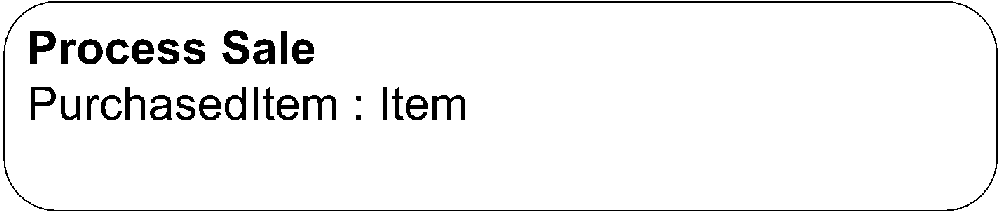
You show an activity as a rectangle with rounded corners. Specify the name of the activity in the upper left. You can show parameters involved in the activity below the name. Alternatively, you can use parameter nodes , described later in this section. Figure 9-1 shows a simple activity.
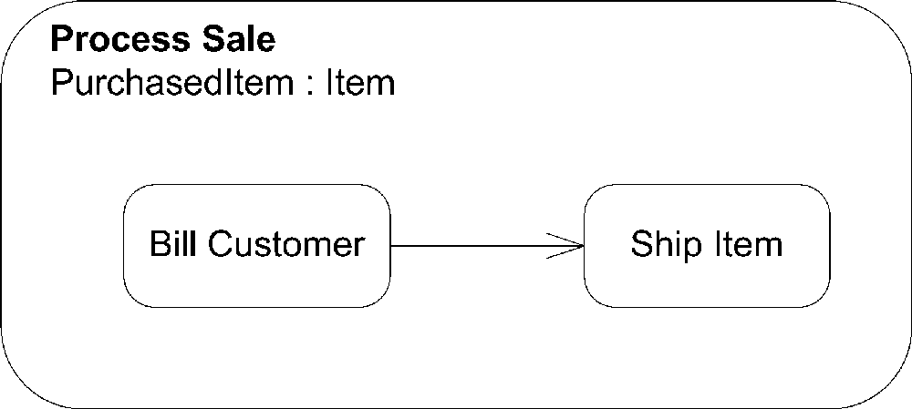
You can show the details for an activity inside of the rectangle, or, to simplify a diagram, leave off the surrounding rectangle altogether. You show actions using the same symbol as an activity: a rectangle with rounded corners; place the name of the action in the rectangle. Figure 9-2 shows some actions inside of an activity.
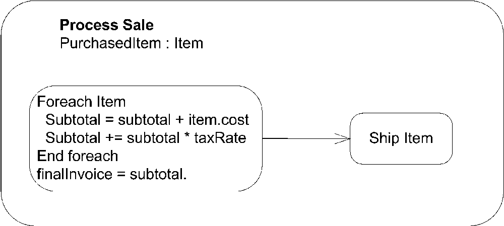
To make activity diagrams more expressive, you can write pseudocode or application-dependent language inside an action. Figure 9-3 shows an example of an action with a domain-specific block of code.
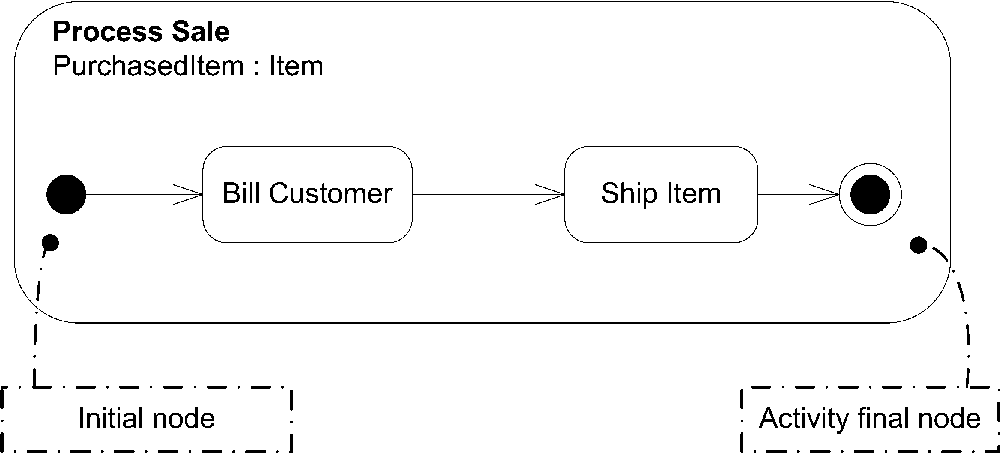
Each activity typically starts with an initial node and ends with an activity final node. When an activity reaches an activity final node, the activity is terminated. You show an initial node as a black dot and an activity final node as a solid circle
with a ring around it. See "Control Nodes" for more information on initial and final nodes. Figure 9-4 shows an activity with initial and final nodes.
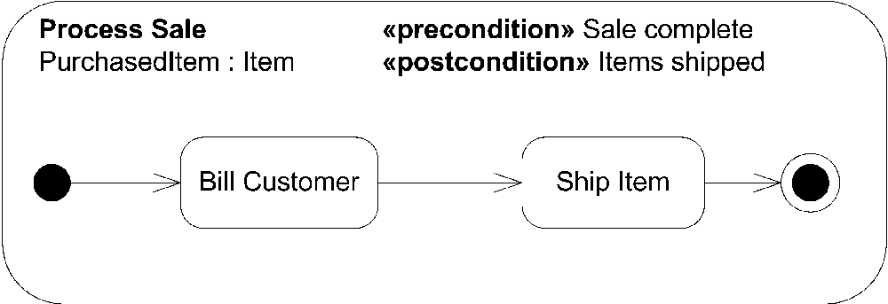
Activities may have pre- and postconditions that apply to the entire activity. You show a precondition by placing the keyword «precondition» at the top center of the activity and then place the constraint immediately after it. You show a post-condition using the keyword «postcondition». Figure 9-5 shows an activity with pre- and postconditions.
An action may have local pre- and postconditions that should hold true before the action is invoked and after it has completed, respectively. However, the UML specification doesn’t dictate how pre- and postconditions map to implementation; violations of the conditions are considered implementation-dependent and don’t necessarily mean the action can’t execute.
You show pre- and postconditions using notes attached to the action. You label the note with the keyword «localPrecondition» or «localPostcondition». Figure 9-6 illustrates this.

Activity Edges
In order to show flow through an activity, you link actions together using activity edges . Edges specify how control and data flow from one action to the next. Actions that aren’t ordered by edges may execute concurrently; the UML specification leaves it up to the specific implementation of an activity diagram to say whether actions actually execute in parallel or are handled sequentially.
You show an activity edge as a line with an arrow pointing to the next action. You can name edges by placing the name near the arrow, though most edges are unnamed. Figure 9-6 (as well as the earlier figures) shows an activity diagram with several activity edges.
Control flows
UML offers a specialized activity edge for control-only elements, called a control flow . A control flow explicitly models control passing from one action to the next. In practice, however, few people make the distinction between a generic activity edge and a control flow because the same notation is used for both.
Object flows
UML offers a data-only activity edge, called object flows . Object flows add support for multicasting data, token selection, and transformation of tokens. The notation for object flows is the same as that for a generic activity edge.
You can use an object flow to select certain tokens to flow from one activity to the next by providing a selection behavior
. You indicate a selection behavior by attaching a note to the object flow with the keyword «selection» and the behavior specified. Figure 9-7 shows selecting the top candidates from potential new hires. See "Object Nodes" for details on modeling objects.

You can assign behaviors to object flows that transform data passed along an edge; however, the behavior can’t have any side effects on the original data. You show transformation behaviors
using a note attached to the object flow. Label the note with the keyword «transformation», and write the behavior under the label. Figure 9-8 shows an example of a transformation behavior that extracts student identification from course registrations to verify that the student’s account is fully paid.
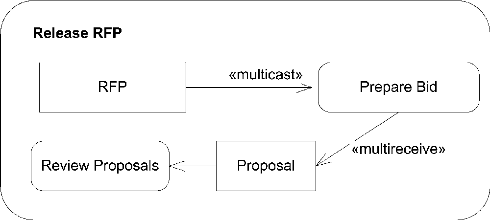
Object flows allow you to specify sending data to multiple instances of a receiver using multicasting. For example, if you are modeling a bidding process, you can show a Request for Proposal (RFP) being sent to multiple vendors and their responses being received by your activity. You show sending data to multiple receivers by labeling an object flow with the keyword «multicast», and you show data being received from multiple senders by labeling an object flow with the keyword «multireceive». Figure 9-9 shows an activity diagram modeling an RFP process.
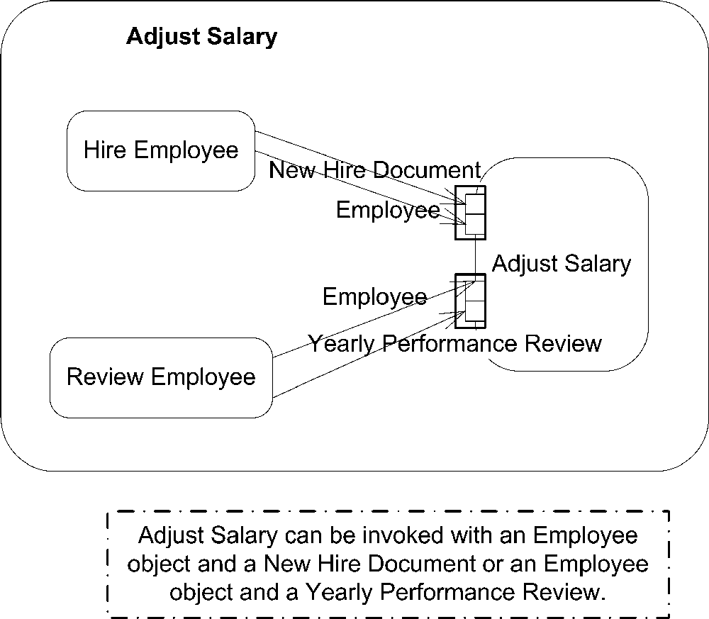
There are times when an action may accept more than one type of valid input to begin execution. For example, a human resources action named Adjust Salary may require an Employee object and either a New Hire Document or Yearly Performance Review Document, but not both. You can show groups and alternatives for input pins (see "Pins" under "Object Nodes“) by using parameter sets
. A parameter set groups one or more pins and indicates that they are all that are needed for starting or finishing an action. An action can use input pins only from one parameter set for any given execution, and likewise output on only one output parameter set. You show a parameter set by drawing a rectangle around

the pins included in the set. Figure 9-10 shows the Adjust Salary action with parameter sets.
Connectors
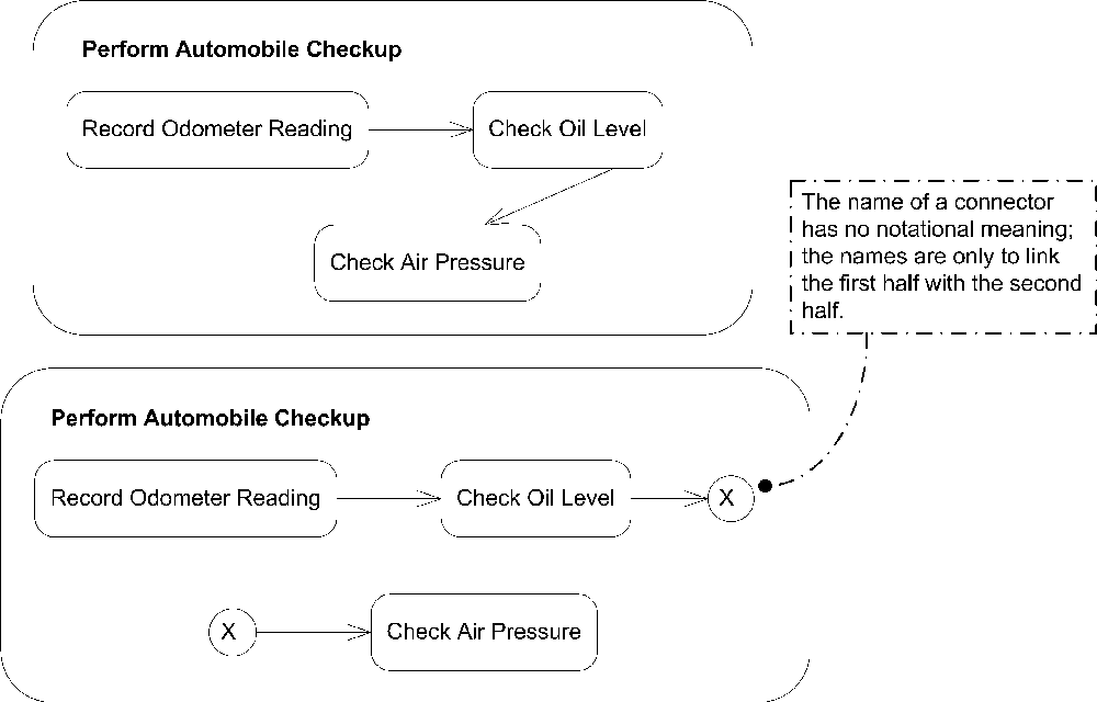
To simplify large activity diagrams you can split edges using connectors. Each connector is given a name and is purely a notational tool. You place the name of a connector in a circle and then show the first half of an edge pointing to the connector and the second half coming out of the connector. Figure 9-11 shows two equivalent activity diagrams; one with a connector and one without.
Tokens
Conceptually, UML models information moving along an edge as a token. A token may represent real data, an object, or the focus of control. An action typically has a set of required inputs and doesn’t begin executing until the inputs are met. Likewise, when an action completes, it typically generates outputs that may trigger other actions to start. The inputs and outputs of an action are represented as tokens .
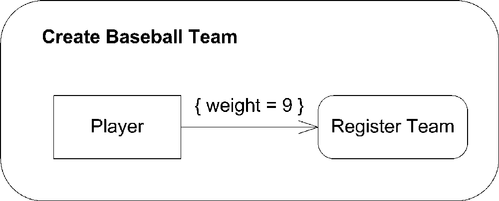
Each edge may have a weight associated with it that indicates how many tokens must be available before the tokens are presented to the target action. You show a weight by placing the keyword weight in curly brackets ({}) equal to the desired number of tokens. A weight of null indicates all tokens should be made available to the target action as soon as they arrive. For example, Figure 9-12 shows that nine players are needed before you can make a baseball team.
In addition to weights, each edge may have a guard condition that is tested against all tokens. If the guard condition fails, the token is destroyed. If the condition passes, the token is available to be consumed by the next action. If a weight is associated with the edge, the tokens aren’t tested against the guard condition until enough tokens are available to satisfy the weight. Each token is tested individually, and if one fails, it is removed from the pool of available tokens. If this reduces the number of tokens available to less than the weight for the edge, all the tokens are held until enough are available. You show a guard condition by putting a boolean expression in brackets ([]) near the activity edge. Guard conditions are typically used with decision nodes to control the flow of an activity (see "Decision and merge nodes“).
Activity Nodes
UML 2.0 defines several types of activity nodes to model different types of information flow. There are parameter nodes to represent data being passed to an activity, object nodes to represent complex data, and control nodes to direct the flow through an activity diagram.
Parameter Nodes
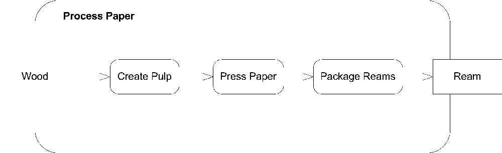
You can represent parameters to an activity or output from an executed activity as parameter nodes . You show a parameter node as a rectangle on the boundary of an activity, with the name or description of the parameter inside the rectangle. Input parameter nodes have edges to the first action, and output parameter nodes have edges coming from the final action to the parameter node. Figure 9-13 shows an example of wood being fed into a paper production activity, and paper being produced at the end.
Object Nodes
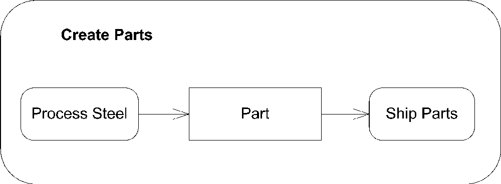
To represent complex data passing through your activity diagram, you can use object nodes. An object node represents an instance of a particular classifier in a certain state. Show an object node as a rectangle, with the name of the node written inside. The name of the node is typically the type of data the node represents. Figure 9-14 is an activity diagram showing a factory producing parts for shipping.
If the type of data the node represents is a signal, draw the node as a concave pentagon. See Figure 9-37 in "Interruptible Activity Regions" for an example of a signal in an activity diagram.
Pins
UML defines a special notation for object nodes, called pins
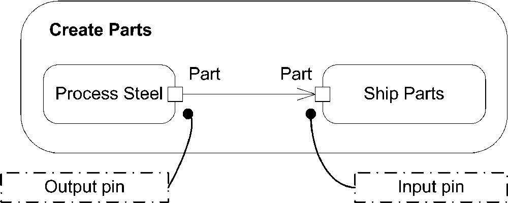
, to provide a shorthand notation for input to or output from an action. For example, because the action Ship Parts in Figure 9-14 requires a Part, you can define an input pin on Ship Parts labeled Part. You show a pin using the same rectangle as for object nodes, except the rectangle is small and attached to the side of its action. If it is an input pin, any edges leading into the action should point to the input pin; if it is an output pin, any edges leaving the action should leave from the pin. Figure 9-15 shows the Create Parts diagram rewritten using pins.
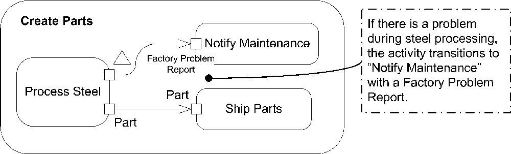
If the output from an action is related to an exception (error condition), you indicate that the pin is an exception pin by inserting a small arrow near the pin. Figure 9-16 shows the Create Parts action with error handling.
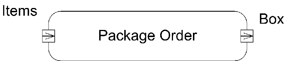
If you don’t have edges leading into or out of an action, you can show whether a pin is an input pin or an output pin by placing small arrows inside the pin rectangle. The arrow should point toward the action if you are showing an input pin and away from the action if you are showing an output pin. Figure 9-17 shows an action with input and output pins.
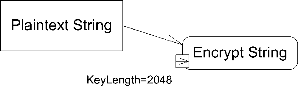
If an action takes a constant value as input, you can model the input data using a value pin . A value pin is shown as a normal input pin, except the value of the object is written near the rectangle. Figure 9-18 shows an activity diagram with a value pin.
Control Nodes
In addition to actions, activities may include other nodes to represent decision making, concurrency, or synchronization. These specialized nodes are called control nodes and are described in detail in this section.
Initial nodes
An initial node is the starting point for an activity; an initial node can have no incoming edges. You can have multiple initial nodes for a single activity to indicate that the activity starts with multiple flows of execution. You show an initial node as a solid black dot, as shown in Figure 9-4.
Decision and merge nodes
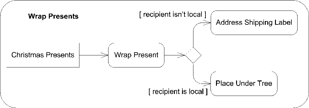
A decision node is a control node that chooses different output flows based on boolean expressions. Each decision node has one input edge and multiple outgoing edges. When data arrives at the decision node, a single outgoing edge is selected, and the data is sent along that edge. A decision node usually selects an edge by evaluating each outgoing edge’s guard condition. A guard condition is a boolean expression that tests some value visible to the activity, typically an attribute of the owning classifier or the data token itself.
You show a decision node as a diamond with the flows coming into or out of the sides. You show guard conditions by putting a boolean expression in brackets ([]) near the activity edge. Figure 9-19 is an activity diagram showing a decision made while wrapping presents.
Guard conditions aren’t guaranteed to be evaluated in any particular order, and a decision node allows only one outgoing edge to be selected. You should take care to design your models so that only one guard condition ever evaluates to true for a given set of data, to prevent race conditions.
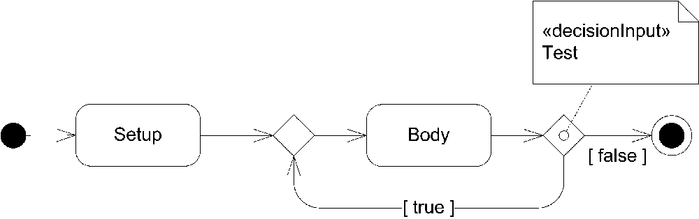
You can specify functionality that executes whenever data arrives at the decision node. Called decision input behavior, this functionality is allowed to evaluate the data arriving at the node and offers output for the guard conditions to evaluate. The behavior is not allowed to have any side effects when executing, since it can
be executed multiple times for the same data input (once for each edge that needs to be tested). You show decision input behavior in a note labeled with the keyword «decisionInput». Figure 9-20 shows an activity diagram that checks to see if a newly authenticated user is the 100th user and should therefore be prompted to take a survey.

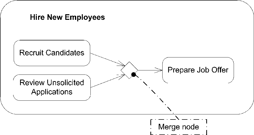
A merge node is effectively the opposite of a decision node; it brings together alternate flows into a single output flow. It doesn’t synchronize multiple concurrent flows; see "Fork and join nodes" for concurrency support. A merge node has multiple incoming edges and a single outgoing edge. A merge node simply takes any tokens offered on any of the incoming edges and makes them available on the outgoing edge.
You show a merge node using the same diamond you use in a decision node, except with multiple incoming edges and a single outgoing edge. Figure 9-21 shows how a potential new hire’s information may be submitted to Human Resources for processing.
Fork and join nodes
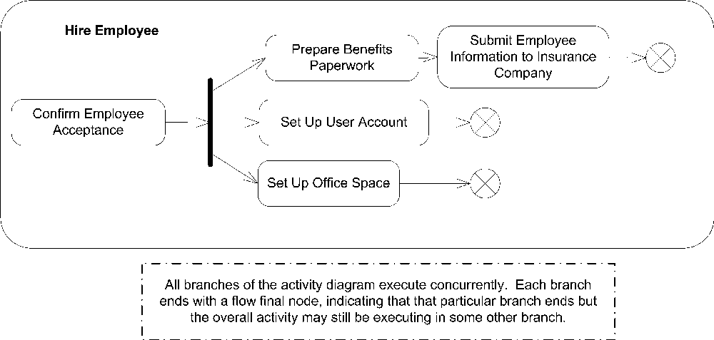
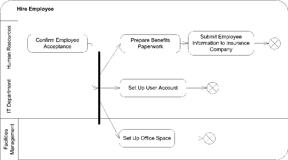
A fork node splits the current flow through an activity into multiple concurrent flows. It has one incoming edge and several outgoing edges. When data arrives at a fork node, it is duplicated for each outgoing edge. For example, you can use a fork node to indicate that when a new person is hired, actions are initiated by Human Resources, the IT Department, and Facilities Management. All these actions execute concurrently and terminate independently.
You show a fork node as a vertical line, with one incoming edge and several outgoing edges. Figure 9-22 is an activity diagram that models hiring a new employee.
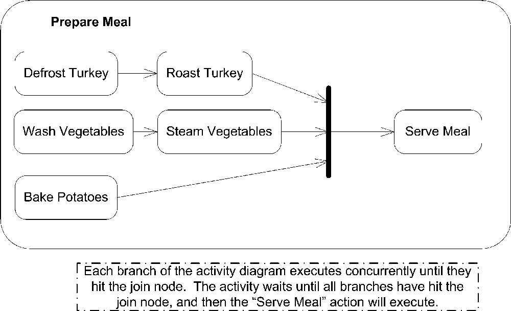
A join node is effectively the opposite of a fork node; it synchronizes multiple flows of an activity back to a single flow of execution. A join node has multiple incoming edges and one outgoing edge. Once all the incoming edges have tokens, the tokens are sent over the outgoing edge.
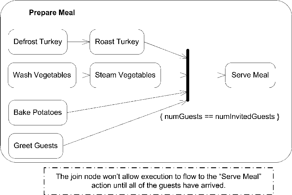
You show a join node as a vertical line, with multiple incoming edges and one outgoing edge. Figure 9-23 is an activity diagram that models serving a meal.
It is worth noting that activity diagrams don’t have the advanced time-modeling notations that interaction diagrams have. So, while it’s possible to show how to prepare a meal and serve everything at the same time with an activity diagram, you can’t capture the time needed to cook each part of the meal. However, you can capture this information with a timing interaction diagram. See Chapter 10 for more information on interaction diagrams.
You can specify a boolean condition to indicate under what conditions the join node will emit a token allowing the flow to continue along its single output edge. This expression is called a join specification
and can use the names of incoming edges and tokens arriving over those edges in the condition. You write a join specification near the join node inside of braces ({}). Figure 9-24 adds greeting guests to the steps involved in preparing a meal and ensures that you don’t serve the meal until all the guests have arrived.
Final nodes
Two types of final nodes are used in activity diagrams: activity final and flow final. Activity final nodes terminate the entire activity. Any tokens that arrive at the activity final node are destroyed, and any execution in any other node is terminated, without results. You can have multiple activity final nodes in a single activity diagram, but a token hitting any of them terminates the whole activity. You show an activity final node as a black dot with a circle around it, as shown in Figure 9-4.
Flow final nodes terminate a path through an activity diagram, but not the entire activity. Flow final nodes are used when the flow of an activity forks, and one
branch of the fork should be stopped but the others may continue. Show a flow final node as a circle with an X in it, as shown in Figure 9-22.
Advanced Activity Modeling
UML 2.0 introduces several powerful modeling notations for activity diagrams that allow you to capture complicated behaviors. Much of this new notation is clearly targeted at moving closer to executable models, with things such as executable regions and exception handling. While not all the notations described in this section are used in every model, these constructs are invaluable when applied correctly.
Activity Partitions
There are times when it is helpful to indicate who (or what) is responsible for a set of actions in an activity diagram. For example, if you are modeling a business process, you can divide an activity diagram by the office or employee responsible for a set of actions. If you are modeling an application, you may want to split an activity diagram based on which tier handles which action. You split an activity diagram using an activity partition. Show an activity partition with two parallel lines, either horizontal or vertical, called swimlanes , with the name of the partition in a box at one end. Place all nodes that execute within the partition between the two lines. Figure 9-25 shows an activity diagram partitioned by business unit.
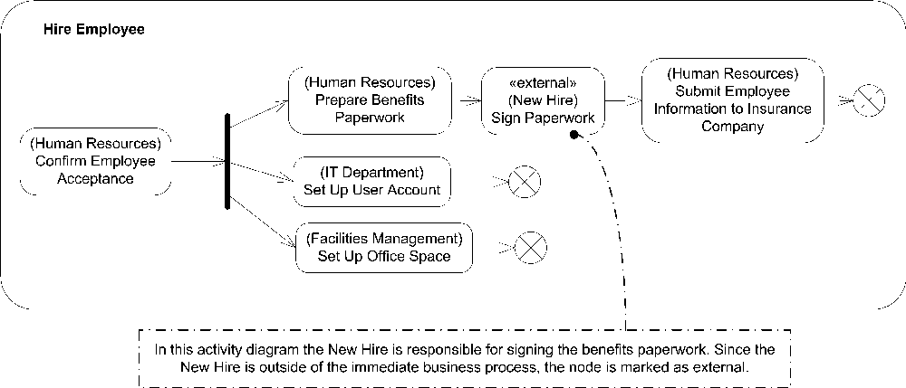
There are times when trying to draw a straight line through your activity diagram may not be possible. You can show that a node is part of a partition by writing the partition name in parentheses above the name of the node. If the activities within
a partition occur outside the scope of your model, you can label a partition with the keyword «external». This is frequently used when performing business modeling using activity diagrams. If the behavior being modeled is handled by someone external to your business process, you can mark the functionality with an external partition. Figure 9-26 shows examples of naming partitions directly on the node and using external partitions.
A partition has no effect on the data flow in an activity, however depending on the entity represented by the partition, there are implications on how actions are handled. If a partition represents a UML classifier, any method invocation within that partition must be handled by an instance of that classifier. If the partition represents an instance, the same restrictions apply, except that behaviors must be handled by the specific instance referenced by the partition. For example, if you are modeling a system that has a partition named LoginService, all actions performed within that partition should be handled by an instance of your LoginService. However, if you have a partition that represents an instance of a User class named CurrentUser, all actions in that partition must be handled by the CurrentUser instance. To indicate that a partition represents a class, you use the keyword «class» before the type name. Though the UML doesn’t explicitly state it, it is customary to show that a partition represents an instance by underlining the type name. Figure 9-27 shows an example of a partition representing a classifier and a partition representing an instance.

Partitions can also represent attributes with specific values. For example, you can have an activity diagram, which shows that at a certain point in its execution, an attribute has a specific value. You can use a partition to indicate the attribute and value available to actions executing within that partition. Indicate that a partition represents an attribute by placing the keyword «attribute», followed by the name of the attribute in a box above the value boxes. Figure 9-28 is an example of an activity diagram in which the UserRole attribute is specified to indicate what level of access a user needs to perform the given actions.
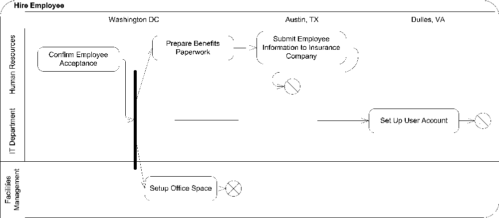
You can combine partitions to show arbitrarily complex constraints on an activity diagram. For example, you can have two partitions that indicate the business department responsible for particular functionality and two partitions indicating the geographic location of the departments. These are called multidimensional partitions and are new to UML 2.0. You can show a multidimensional partition by using both horizontal and vertical intersecting partitions, as shown in Figure 9-29.
Exception Handling
UML 2.0 activity diagrams provide support for modeling exception handling. An exception is an error condition that occurs during the execution of an activity. An exception is said to be thrown by the source of the error and caught when it is handled. You can specify that an action can catch an exception by defining an exception handler. The exception handler defines the type of exception, and a behavior to execute when that particular exception is caught.

You show an exception handler as a regular node with a small square on its boundary. Draw a lightning-bolt-style edge from the protected node to the small square. Finally, label the edge with the type of the exception caught by this handler. Figure 9-30 shows an example exception handler.
If an exception occurs while an action is executing, the execution is abandoned and there is no output from the action. If the action has an exception handler, the handler is executed with the exception information. When the exception handler executes, its output is available to the next action after the protected node, as though the protected node had finished execution.
If the action doesn’t have an exception handler, the exception propagates to outer nodes until it encounters an exception handler. As the exception leaves a node (an action, structured activity node, or activity) all processing in the node is terminated. It is unspecified what happens if the exception makes it to the top level of a system without being caught; UML 2.0 profiles can define specific behavior to handle this.

Expansion Regions
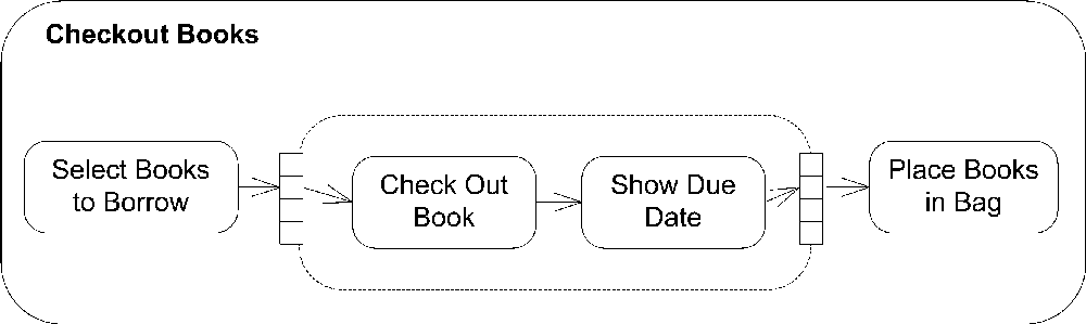
You can show that an action, or set of actions, executes over a collection of input data by placing the actions in an expansion region. For example, if you had an action named Check Out Books that checked each of the provided books out of a library, you can model the checkout book action using an expansion region, with a collection of books as input.
You show an expansion region using a dashed rectangle, with rounded corners surrounding the actions that should execute for each piece of input data. Place a row of four input pins on the dashed boundary to represent a collection of data coming into the region. You show a line with an arrow to the row of input pins, and then from the input pins to the input pin of the first internal action. Likewise, you show a row of four output pins on the dashed boundary, with edges coming from the last action’s output pin to the row of four output pins on the region. Figure 9-31 shows the Check Out Book expansion region.
The use of four input pins simply represents a collection of input data; it doesn’t specify how much data is actually presented to the expansion region. The region executes for each piece of data in the collection and, assuming there are no errors, offers one piece of output data from each execution.
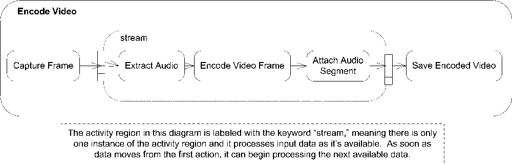
You can use the keywords «parallel», «iterative», or «stream» to indicate if the executions of the expansion region can occur concurrently (parallel), sequentially (iterative), or continuously (stream). Place the keyword in the upper left of the expansion region. Figure 9-32 shows a video encoder that streams the frames through the various stages of encoding as soon as they are available.
Looping
UML 2.0 defines a construct to model looping in activity diagrams. A loop node has three subregions: setup, body, and test. The test subregion may be evaluated before or after the body subregion. The setup subregion executes only once, when first entering the loop; the test and body sections execute each time through the loop until the test subregion evaluates to false.
The specification gives no suggested notation for loop nodes, however you can improvise one using activity regions. Conceptually, a loop node looks like Figure 9-33.
Using activity partitions, you can express this as a single node, as shown in Figure 9-34.

Streaming
An action is said to be streaming if it can produce output while it is processing input. For example, an action representing a compression algorithm can take audio input data from a streamed input and send compressed audio along a streamed output.
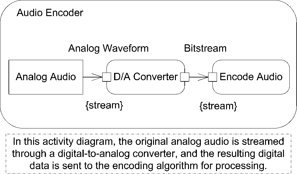
You indicate that an action is streaming its input and output by placing the keyword stream in braces ({}) near the edges coming in and out of an action. Figure 9-35 shows an example audio encoding that is streaming data.
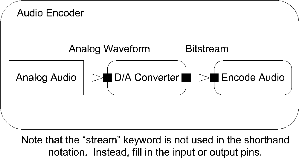
UML provides a shorthand notation for streaming edges, and input and output pins: use a solid arrowhead or rectangle. Figure 9-36 shows the same audio encoder, but is drawn using the streaming shorthand notation.
The UML specification expects that vendors will provide base classes for domain-specific activities users can employ to model an application-specific problem. You may also mark a set of actions as streaming using an expansion region. See "Expansion Regions" for more information.
Interruptible Activity Regions
You can mark that a region of your activity diagram can support termination of the tokens and processing by marking it as an interruptible activity region. For example, you may want to make a potentially long-running database query as interruptible so that the user can terminate things if he doesn’t want to wait for the results.
You indicate a region is interruptible by surrounding the relevant nodes with a dashed rectangle that has rounded corners. You indicate how the region can be interrupted by drawing a lightning-bolt-style edge leaving the region and connecting to the node that assumes execution. If a token leaves the region over this edge, all other processing and tokens inside the region are terminated. The token leaving the region is unaffected.
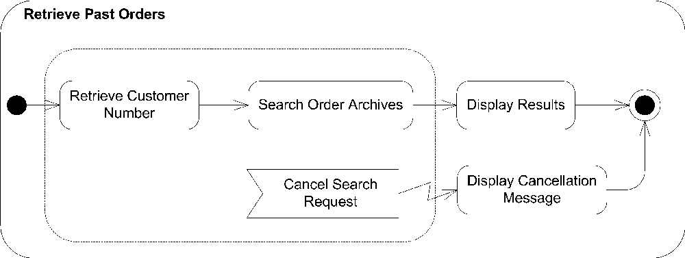
Typically the source of an interruption is the receipt of a signal from an external entity. You show receipt of a signal as a concave pentagon, with the name of the signal inside. Figure 9-37 shows an example of a long-running database query being interrupted by user input.
Central Buffer Nodes
UML 2.0 introduced a new type of activity node, called the central buffer node, that provides a place to specify queuing functionality for data passing between object nodes. A central buffer node takes inputs from several object node sources and offers them along several object node outputs. For example, there may be two car-manufacturing plants feeding a car dealer supply line. A central buffer node can be placed between the manufacturing plants and the dealers to specify prioritization of deliveries or sorting of the manufactured cars. You show a central buffer node as a rectangle with the keyword «centralBuffer» at the top and the
type of object written in the center. Figure 9-38 shows an example central buffer node feeding car dealer supply lines.

Data Store Nodes
A data store node is a special type of central buffer node that copies all data that passes through it. For example, you can insert a data store node in your activity diagram to indicate that all interactions are logged to an external database, or that when an article is submitted for review, it is automatically stored in a searchable archive.
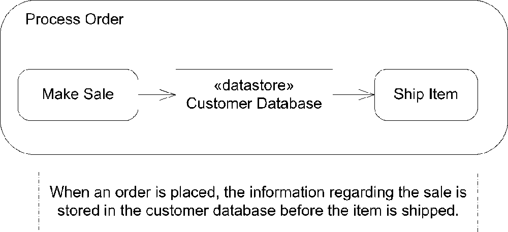
You show a data store node as a stereotyped version of an object node. Show the node as a rectangle, and place the keyword «datastore» above the name of the node. Figure 9-39 shows a data store node.
If the same object passes through a data store node, the specification states that the previous version of the object will be overwritten.
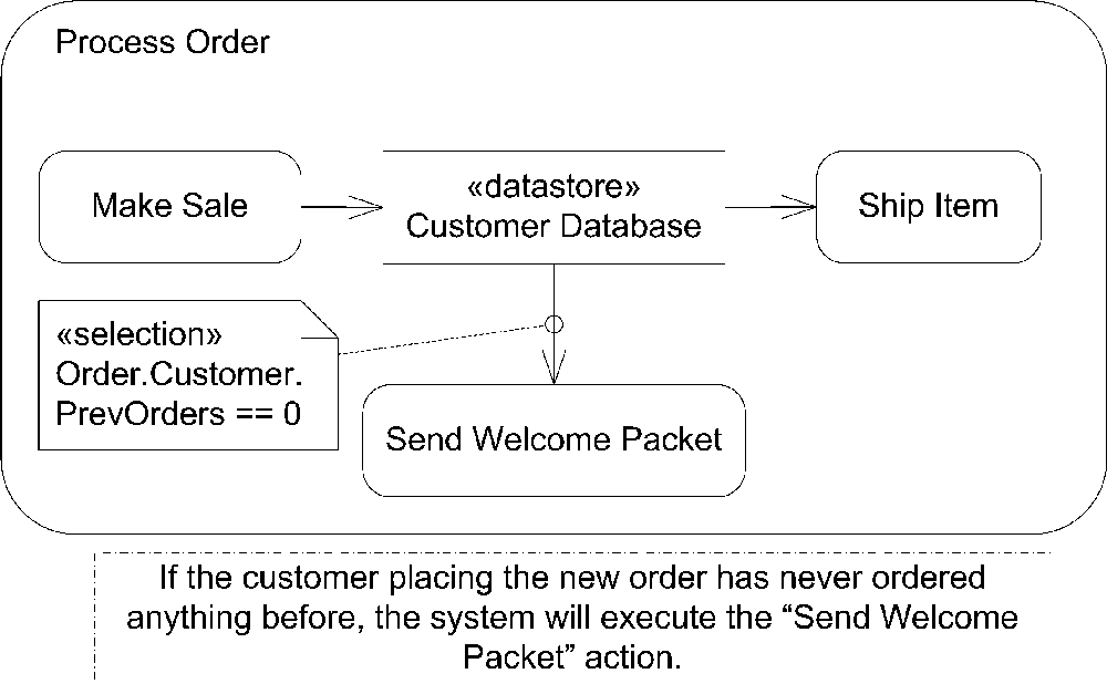
You can show transitions from a data store node that have additional information to select a subset of the data stored in a data store node, similar to a database query. The specification doesn’t require any particular syntax and suggests showing the selection criteria in a note labeled with the keyword «selection». Figure 9-40 shows an activity diagram that uses a data store node to send welcome packets to new customers.