3

Higher-Order Models in Computer Vision

Pushmeet Kohli

Machine Learning and Perception
Microsoft Research
Cambridge, UK

Email: [email protected]

Carsten Rother

Machine Learning and Perception
Microsoft Research
Cambridge, UK

Email: [email protected]

CONTENTS

3.1    Introduction

3.1.1    Outline

3.2    Higher-Order Random Fields

3.3    Patch and Region-Based Potentials

3.3.1    Label Consistency in a Set of Variables

3.3.2    Pattern-Based Potentials

3.4    Relating Appearance Models and Region-Based Potentials

3.5    Global Potentials

3.5.1    Connectivity Constraint

3.5.2    Constraints and Priors on Label Statistics

3.6    Maximum a Posteriori Inference

3.6.1    Transformation-Based Methods

3.6.2    Dual Decomposition

3.7    Conclusions and Discussion

Bibliography

3.1    Introduction

Many computer vision problems such as object segmentation, disparity estimation, and 3D reconstruction can be formulated as pixel or voxel labeling problems. The conventional methods for solving these problems use pairwise conditional and markov random field (CRF/MRF) formulations [1], which allow for the exact or approximate inference of maximum a posteriori (MAP) solutions. MAP inference is performed using extremely efficient algorithms such as combinatorial methods (e.g., graph-cut [2, 3, 4] or the BHS-algorithm [5, 6]), or message passing-based techniques (e.g., belief propagation (BP) [7, 8, 9] or tree-reweighted (TRW) message passing [10, 11]).

The classical formulations for image-labeling problems represent all output elements using random variables. An example is the problem of interactive object cutout where each pixel is represented using a random variable which can take two possible labels: foreground or background. The conventionally used pairwise random field models introduce a statistical relationship between pairs of random variables, often only among the immediate 4 or 8 neighboring pixels. Although such models permit efficient inference, they have restricted expressive power. In particular, they are unable to enforce the high-level structural dependencies between pixels that have been shown to be extremely powerful for image-labeling problems. For instance, while segmenting an object in 2D or 3D, we might know that all its pixels (or parts) are connected. Standard pairwise MRFs or CRFs are not able to guarantee that their solutions satisfy such a constraint. To overcome this problem, a global potential function is needed which assigns all such invalid solutions a zero probability or an infinite energy.

Despite substantial work from several communities, pairwise MRF and CRF models for computer vision problems have not been able to solve image-labeling problems such as object segmentation fully. This has led researchers to question the richness of these classical pairwise energy-function-based formulations, which in turn has motivated the development of more sophisticated models. Along these lines, many have turned to the use of higher-order models that are more expressive, thereby enabling the capture of statistics of natural images more closely.

The last few years have seen the successful application of higher-order CRFs and MRFs to some low-level vision problems such as image restoration, disparity estimation and object segmentation [12, 13, 14, 15, 16, 17, 18, 19, 20, 21, 22, 23]. Researchers have used models composed of new families of higher-order potentials, i.e., potentials defined over multiple variables, which have higher modeling power and lead to more accurate models of the problem. Researchers have also investigated incorporation of constraints such as connectivity of the segmentation in CRF and MRF models. This is done by including higher-order or global potentials¹ that assign zero probability (infinite cost) to all label configurations that do not satisfy these constraints.

One of the key challenges with respect to higher-order models is the question of efficiently inferring the Maximum a Posterior (MAP) solution. Since, inference in pairwise models is very well studied, one popular technique is to transform the problem back to a pairwise random field. Interestingly, any higher-order function can be converted to a pairwise one, by introducing additional auxiliary random variables [5, 24]. Unfortunately, the number of auxiliary variables grows exponentially with the arity of the higher-order function, hence in practice only higher-order function with a few variables can be handled efficiently. However, if the higher-order function contains some inherent “structure”, then it is indeed possible to practically perform MAP inference in a higher-order random field where each higher-order function may act on thousands of variables [25, 15, 26, 21]. We will review various examples of such potential functions in this chapter.

There is a close relationship between higher-order random fields and random field models containing latent variables [27, 19]. In fact, as we will see later in the chapter, any higher-order model can be written as a pairwise model with auxiliary latent variables and vice versa [27]. Such transformations enable the use of powerful optimization algorithms and even result in global optimally solutions for some problem instances. We will explain the connection between higher-order models and models containing latent variables, using the problem of interactive foreground/background image segmentation as an example [28, 29].

3.1.1    Outline

This chapter deals with higher-order graphical models and their applications. We discuss a number of recently proposed higher-order random field models and the associated algorithms that have been developed to perform MAP inference in them. The structure of the chapter is as follows.

We start with a brief introduction of higher-order models in Section 3.2. In Section 3.3, we introduce a class of higher-order functions which encode interactions between pixels belonging to image patches or regions. In Section 3.4 we relate the conventional latent variable CRF model for interactive image segmentation [28] to a random field model with region-based higher-order functions. Section 3.5 discusses models which encode image-wide (global) constraints. In particular, we discuss the problem of image segmentation under a connectivity constraint and solving labeling problems under constraints on label-statistics. In Section 3.6, we discuss algorithms that have been used to perform MAP inference in such models. We concentrate on two categories of techniques: the transformation approach, and the problem (dual) decomposition approach. We also give pointers to many other inference techniques for higher-order random fields such as message passing [18, 21]. For topics on higher-order model that are not discussed in this chapter, we refer the reader to [30, 31].

3.2    Higher-Order Random Fields

Before proceeding further, we provide the basic notation and definitions used in this chapter. A random field is defined over a set of random variables x = {xi|i ∈ V}x = {xi|i ∈ V}$x=\left\{x_i\text{|}i\in \mathcal{V}\right\}$. These variables are typically arranged on a lattice $\mathcal{V}=\left\{1,2,\dots ,n\right\}$ and represent scene elements, such as pixels or voxels. Each random variable takes a value from the label set $ℒ=\left\{l_1,l_2,\dots ,l_k\right\}$. For example, in scene segmentation, the labels can represent semantic classes such as a building, tree, or a person. Any possible assignment of labels to the random variables will be called a labeling (also denoted by x). Clearly, in the above scenario the total number of labelings x is kⁿ.

An MRF or CRF model enforces a particular factorization of the posterior distribution P(x|d), where d is the observed data (e.g., RGB input image). It is common to define an MRF or CRF model through its so-called Gibbs energy function E(x), which is the negative log of the posterior distribution of the random field, i.e.,

$E\left(x;d\right)=-\log P\left(x\text{|}d\right)+\text{constant}.$

(3.1)

The energy (cost) of a labeling x is represented as a sum of potential functions, each of which depends on a subset of random variables. In its most general form, the energy function can be defines as:

$E\left(x;d\right)={\displaystyle \sum _{c\in \mathcal{C}}{\psi }_c\left(x_c\right)}.$

(3.2)

Here, c is called a clique which is a set of random variables x_c which are conditionally dependent on each other. The term ψ_c(x_c) denotes the value of the clique potential corresponding to the labeling x_c ⊆ x for the clique c, and $\mathcal{C}$ is the set of all cliques. The degree of the potential ψ_c(·) is the size of the corresponding clique c (denoted by |c|). For example, a pairwise potential has |c| = 2.

For the well-studied special case of pairwise MRFs, the energy only consists of potentials of degree one and two, that is,

$E\left(x;d\right)={\displaystyle \sum _{i\in \mathcal{V}}{\psi }_i\left(x_i;d\right)}+{\displaystyle \sum _{\left(i,j\right)\in ℰ}{\psi }_{ij}\left(x_i,x_j\right).}$

(3.3)

Here, $ℰ$ represents the set of pairs of variables which interact with each other. In the case of image segmentation, $ℰ$ may encode a 4-connected neighborhood system on the pixel-lattice.

Observe that the pairwise potential ψ_ij(x_i, x_j) in Equation 3.3 does not depend on the image data. If we condition the pairwise potentials on the data, then we obtain a pairwise CRF model which is defined as:

$E\left(x;d\right)={\displaystyle \sum _{i\in \mathcal{V}}{\psi }_i\left(x_i;d\right)}+{\displaystyle \sum _{\left(i,j\right)\in ℰ}{\psi }_{ij}}\left(x_i,x_j;d\right).$

(3.4)

3.3    Patch and Region-Based Potentials

In general, it is computationally infeasible to exactly represent a general higher order potential function defined over many variables². Some researchers have proposed higher-order models for vision problems which use potentials defined over a relatively small number of variables. Examples of such models include the work of Woodford et al. [23] on disparity estimation using a third-order smoothness potential, and El-Zehiry and Grady [12] on image segmentation with a curvature potential³. In such cases, it is also feasible to transform the higher-order energy into an equivalent pairwise energy function with the addition of a relatively small number of auxiliary variables, and minimize the resulting pairwise energy using conventional energy minimization algorithms.

Although the above-mentioned approach has been shown to produce good results, it is not able to deal with higher-order potentials defined over a very large number (hundreds or thousands) of variables. In the following, we present two categories of higher-order potentials that can be represented compactly and minimized efficiently. The first category encodes the property that pixels belonging to certain groups take the same label. While this is a powerful concept in several application domains, e.g., pixel-level object recognition, it is not always applicable, e.g., image denoising. The second category generalizes this idea by allowing groups of pixels to take arbitrary labelings, as long as the set of different labelings is small.

3.3.1    Label Consistency in a Set of Variables

A common method to solve various image-labeling problems like object segmentation, stereo and single view reconstruction is to formulate them using image segments (so-called superpixels [33]) obtained from unsupervised segmentation algorithms. Researchers working with these methods have made the observation that all pixels constituting the segments often have the same label, that is, they might belong to the same object or might have the same depth.

Standard super-pixel based methods use label consistency in super-pixels as a hard constraint. Kohli et al. [25] proposed a higher-order CRF model for image labeling that used label consistency in superpixels as a soft constraint. This was done by using higher-order potentials defined on the image segments generated using unsupervised segmentation algorithms. Specifically, they extend the standard pairwise CRF model often used for object segmentation by incorporating higher-order potentials defined on sets or regions of pixels. In particular, they extend the pairwise CRF which is used in TextonBoost [34]⁴.

The Gibbs energy of the higher-order CRF of [25] can be written as:

$E\left(x\right)={\displaystyle \sum _{i\in \mathcal{V}}{\psi }_i\left(x_i\right)}+{\displaystyle \sum _{\left(i,j\right)\in ℰ}{\psi }_{ij}}\left(x_i,x_j\right)+{\displaystyle \sum _{c\in \mathcal{S}}{\psi }_c}\left(x_c\right),$

(3.5)

where $ℰ$ represents the set of all edges in a 4- or 8-connecting neighborhood system, $\mathcal{S}$ refers to a set of image segments (or superpixels), and ψ_c are higher-order label consistency potentials defined on them. In [25], the set $\mathcal{S}$ consisted of all segments of multiple segmentations of an image obtained using an unsupervised image segmentation algorithm such as mean-shift [35]. The labels constituting the label set $ℒ$ of the CRF represent the different objects. Every possible assignment of the random variables x (or configuration of the CRF) defines a segmentation.

The label consistency potential used in [25] is similar to the smoothness prior present in pairwise CRFs [36]. It favors all pixels belonging to a segment taking the same label. It takes the form of a Pⁿ Potts model [15]:

${\psi }_c\left(x_c\right)=\{\begin{array}{ccc}0& \text{if}& x_i=l_k,\forall i\in c,\\ {\theta }_1{\left|c\right|}^{{\theta }_{\alpha }}& \text{otherwise}.& \end{array}$

(3.6)

where |c| is the cardinality of the pixel set c⁵, and θ₁ and θ_α are parameters of the model. The expression θ₁|c|^θ_α gives the label inconsistency cost, i.e., the cost added to the energy of a labeling in which different labels have been assigned to the pixels constituting the segment. Figure 3.1(left) visualizes a Pⁿ Potts potential.

The Pⁿ Potts model enforces label consistency rigidly. For instance, if all but one of the pixels in a superpixel take the same label then the same penalty is incurred as if they were all to take different labels. Due to this strict penalty, the potential might not be able to deal with inaccurate super-pixels or resolve conflicts between overlapping regions of pixels. Kohli et al. [25] resolved this problem by using the Robust higher-order potentials defined as:

${\psi }_c\left(x_c\right)=\{\begin{array}{cc}{N}_i\left(x_c\right)\frac{1}{Q}{\gamma }_{\max }& \text{if}{N}_i\left(x_c\right)\le Q\\ {\gamma }_{\max }& \text{otherwise}.\end{array}$

(3.7)

where N_i(x_c) denotes the number of variables in the clique c not taking the dominant label, i.e., N_i(x_c) = min_k(|c| – n_k(x_c)), γ_max = |c|^θ_α(θ₁ + θ₂G(c)), where G(c) is the measure of the quality of the superpixel c, and Q is the truncation parameter, which controls the rigidity of the higher-order clique potential. Figure 3.1(right) visualizes a robust Pⁿ Potts potential.

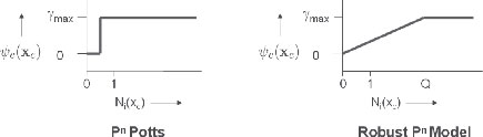
FIGURE 3.1
Behavior of the rigid Pⁿ Potts potential (left) and the Robust Pⁿ model potential (right). The figure shows how the cost enforced by the two higher-order potentials changes with the number of variables in the clique not taking the dominant label, i.e., N_i(x_c) = min_k(|c| − n_k(x_c)), where n_k (.) returns the number of variables x_i in x_c that take the label k. Q is the truncation parameter used in the definition of the higher-order potential (see equation 3.7).

Unlike the standard Pⁿ Potts model, this potential function gives rise to a cost that is a linear truncated function of the number of inconsistent variables (see Figure 3.1). This enables the robust potential to allow some variables in the clique to take different labels. Figure 3.2 shows results for different models.

Lower-Envelope Representation of Higher-Order Functions

Kohli and Kumar [24] showed that many types of higher-order potentials including the Robust Pⁿ model can be represented as lower envelopes of linear functions. They also showed that the minimization of such potentials can be transformed to the problem of minimizing a pairwise energy function with the addition of a small number of auxiliary variables which take values from a small label set.

It can be easily seen that the Robust Pⁿ model (3.7) can be written as a lower envelope potential using h + 1 linear functions. The functions $f^q,q\in \mathcal{Q}=\left\{1,2,\dots ,h+1\right\}$ are defined using

$\begin{array}{l}{\mu }^q=\{\begin{array}{ll}\hfill {\gamma }_a\hfill & \text{if}q=a\in ℒ,\hfill \\ \hfill {\gamma }_{\max }\hfill & \text{otherwise},\hfill \end{array}\hfill \\ w_{ia}^q=\{\begin{array}{cc}0\hfill & \text{if}q=h+1\text{or}a=q\in ℒ,\hfill \\ \hfill {\alpha }_a\hfill & \text{otherwise}\text{.}\hfill \end{array}\hfill \end{array}$

The above formulation is illustrated in Figure 3.3 for the case of binary variables.

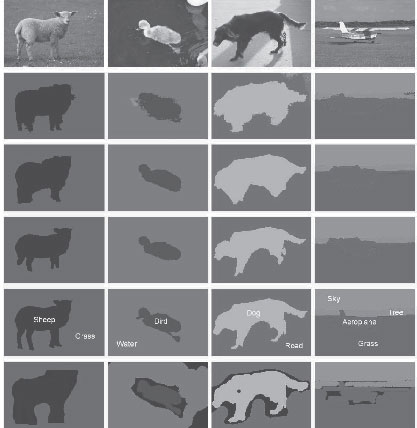
FIGURE 3.2
Some qualitative results. Please view in colour. First row: Original image. Second row: Unary likelihood labeling from TextonBoost [34]. Third row: Result obtained using a pairwise contrast preserving smoothness potential as described in [34]. Fourth row: Result obtained using the Pⁿ Potts model potential [15]. Fifth row: Results using the Robust Pⁿ model potential (3.7) with truncation parameter Q = 0.1|c|, where |c| is equal to the size of the super-pixel over which the Robust Pⁿ higher-order potential is defined. Sixth row: Hand-labeled segmentations. The ground truth segmentation are not perfect and many pixels (marked black) are unlabelled. Observe that the Robust Pⁿ model gives best results. For instance, the leg of the sheep and bird have been accurately labeled, which was missing in the other results.

3.3.2    Pattern-Based Potentials

The potentials in the previous section were motivated by the fact that often a group of pixels have the same labeling. While this is true for a group of pixels which is inside an object, it is violated for a group which encodes a transitions between objects. Furthermore, the label consistency assumption is also not useful when the labeling represents, e.g., natural textures. In the following we will generalize the label-consistency potentials to so-called pattern-based potentials, which can model arbitrary labelings. Unfortunately, this generalization also implies that the underlying optimization will become harder (see Section 3.6).

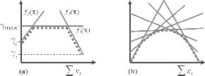
FIGURE 3.3
(a) Robust Pⁿ model for binary variables. The linear functions f₁ and f₂ represents the penalty for variables not taking the labels 0 and 1, respectively. The function f₃ represents the robust truncation factor. (b) The general concave form of the robust Pⁿ model defined using a larger number of linear functions.

Suppose we had a dictionary containing all possible 10 × 10 patches that are present in natural real-world images. One could use this dictionary to define a higher-order prior for the image restoration problem which can be incorporated in the standard MRF formulation. This higher-order potential is defined over sets of variables, where each set corresponds to a 10 × 10 image patch. It enforces that patches in the restored image come from the set of natural image patches. In other words, the potential function assigns a low cost (or energy) to the labelings that appear in the dictionary of natural patches. The rest of the labelings are given a high (almost constant) cost.

It is well known that only a small fraction of all possible labelings of a 10 × 10 patch actually appear in natural images. Rother et al. [26] used this sparsity property to compactly represent a higher-order potential prior for binary texture denoising by storing only the labelings that need to be assigned a low cost, and assigning a (constant) high cost to all other labelings.

They parameterize higher-order potentials by a list of possible labelings (also called patterns [37]) $\mathcal{X}=\left\{X_1,X_2,\dots ,X_t\right\}$ of the clique variables x_c, and their corresponding costs θ = {θ₁, θ₂, …, θ_t}. They also include a high constant cost θ_max for all other labelings. Formally, the potential functions can be defined as:

${\psi }_c\left(x_c\right)=\{\begin{array}{cc}{\theta }_q& \text{if}{x}_c=X_q\in \mathcal{X}\\ {\theta }_{\max }& \text{otherwise},\end{array}$

(3.8)

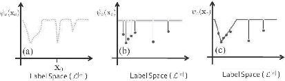
FIGURE 3.4
Different parameterizations of higher-order potentials. (a) The original higher-order potential function. (b) Approximating pattern-based potential which requires the definition of 7 labelings. (c) The compact representation of the higher-order function using the functional form defined in Equation (3.9). This representation (3.9) requires only t = 3 deviation functions.

where θ_q ≤ θ_max, ∀θ_q ∈ θ. The higher-order potential is illustrated in Figure 3.4(b). This representation was concurrently proposed by Komodakis et al. [37].

Soft Pattern Potentials

The pattern-based potential is compactly represented and allows efficient inference. However, the computation cost is still quite high for potentials which assign a low cost to many labelings. Notice that the pattern-based representation requires one pattern per low-cost labeling. This representation cannot be used for higher-order potentials where a large number of labelings of the clique variables are assigned low weights (< θ_max).

Rother et al. [26] observed that many low-cost label assignments tend to be close to each other in terms of the difference between labelings of pixels. For instance, consider the image segmentation task, which has two labels, foreground (f) and background (b). It is conceivable that the cost of a segmentation labeling (fffb) for 4 adjacent pixels on a line would be close to the cost of the labeling (ffbb). This motivated them to try to encode the cost of such groups of similar labelings in the higher-order potential in such a way that their transformation to quadratic functions does not require increasing the number of states of the switching variable z (see details in Section 3.6). The differences of the representations are illustrated in Figure 3.4(b) and (c).

They parameterized the compact higher-order potentials by a list of labeling deviation cost functions $\mathcal{D}=\left\{d_1,d_2,\dots ,d_t\right\}$, and a list of associated costs θ = {θ₁, θ₂, …, θ_t}. They also maintain a parameter for the maximum cost θ_max that the potential can assign to any labeling. The deviation cost functions encode how the cost changes as the labeling moves away from some desired labeling. Formally, the potential functions can be defined as:

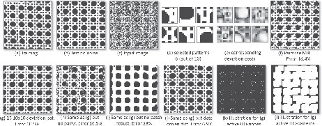
FIGURE 3.5
Binary texture restoration for Brodatz texture D101. (a) Training image (86 × 86 pixels). (b) Test image. (c) Test image with 60% noise, used as input. (d) 6 (out of 10) selected patterns of size 10 × 10 pixels. (e) Their corresponding deviation cost function. (f–j) Results of various different models (see text for details).

${\psi }_c\left(x_c\right)=\min \left\{\underset{q\in \left\{1,2,\dots ,t\right\}}{\min }{\theta }_q+d_q\left(x_c\right),{\theta }_{\max }\right\},$

(3.9)

where deviation functions $d_q:{ℒ}^{\left|c\right|}\to ℝ$ are defined as: $d_q\left(x_c\right)={\displaystyle {\sum }_{i\in c;l\in ℒ}{w}_{il}^q\delta \left(x_i=l\right)}$, where $w_{il}^q$ is the cost added to the deviation function if variable x_i of the clique c is assigned label l. The function δ(x_i = l) is the Kronecker delta function that returns value 1 if x_i = l and returns 0 for all assignments of x_i. This higher-order potential is illustrated in Figure 3.4(c). It should be noted that the higher-order potential (3.9) is a generalization of the pattern-based potential defined in Equation (3.8) and in [37]. Setting weights $w_{il}^q$ as:

$w_{il}^q=\{\begin{array}{ll}\hfill 0\hfill & \text{if}{X}_q\left(i\right)=l\hfill \\ \hfill {\theta }_{\max }\hfill & \text{otherwise}\hfill \end{array}$

(3.10)

makes potential (3.9) equivalent to Equation (3.8).

Note, that the above pattern-based potentials can also be used to model arbitrary higher-order potentials, as done in, e.g., [38], as long as the size of the clique is small.

Pattern-Based Higher-Order Potentials for Binary Texture Denoising

Pattern-based potentials are especially important for computer vision since many image labeling problems in vision are dependent on good prior models of patch labelings. In existing systems, such as new view synthesis, e.g., [13], or super-resolution, e.g., [39], patch-based priors are used in approximate ways and do not directly solve the underlying higher-order random field.

Rother et al. [26] demonstrated the power of the pattern-based potentials for the toy task of denoising a specific type of binary texture, i.e., Brodatz texture D101⁶. Given a training image, Figure 3.5(a), their goal was to denoise the input image (c) to achieve ideally (b). To derive the higher-order potentials, they selected a few patterns of size 10 × 10 pixels, which occur frequently in the training image (a) and are as different as possible in terms of their Hamming distance. They achieve this by k-means clustering over all training patches. Figure 3.5(d) depicts 6 (out of k = 10) such patterns.

6  This specific denoising problem has also been addressed previously in [40].

To compute the deviation function for each particular pattern, they considered all patterns that belong to the same cluster. For each position within the patch, they record the frequency of having the same value. Figure 3.5(e) shows the associate deviation costs, where a bright value means low frequency (i.e., high cost). As expected, lower costs are at the edge of the pattern. Note, the scale and truncation of the deviation functions, as well as the weight of the higher-order function with respect to unary and pairwise terms, are set by hand in order to achieve best performance. The results for various models are shown in Figure 3.5(f–l). (Please refer to [26] for a detailed description of each model.)

Figure 3.5(f) shows the result with a learned pairwise MRF. It is apparent that the structure on the patch-level is not preserved. In contrast, the result in Figure 3.5(g), which uses the soft higher-order potentials and pairwise function, is clearly superior. Figure 3.5(h) shows the result with the same model as in (g) but where pairwise terms are switched off. The result is not as good since those pixels which are not covered by a patch are unconstrained and hence take the optimal noisy labeling. Figure 3.5(i) shows the importance of having patch robustness, i.e., that θ_max in Equation (3.9) is not infinite, which is missing in the classical patch-based approaches (see [26]). Finally, 3.5(j) shows a result with the same model as in (g) but with a different dictionary. In this case the 15 representative patches are different for each position in the image. To achieve this, they used the noisy input image and hence have a CRF model instead of an MRF model (see details in [26]).

Figure 3.5(k-l) visualizes the energy for the result in (g). In particular, 3.5(k) illustrates in black those pixels where the maximum (robustness) patch cost θ_max is paid. It can be observed that only a few pixels do not utilize the maximum cost. Figure 3.5(1) illustrates all 10 × 10 patches that are utilized, i.e., each white dot in 3.5(k) relates to a patch. Note that there is no area in 3.5(1) where a patch could be used that does not overlap with any other patch. Also, note that many patches do overlap.

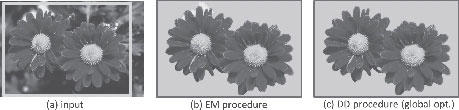
FIGURE 3.6
Interactive image segmentation using the interactive segmentation method proposed in [29]. The user places a yellow rectangle around the object (a). The result (b) is achieved with the iterative EM-style procedure proposed [29]. The result (c) is the global optimum of the function, which is achieved by transforming the energy to a higher-order random field and applying a dual-decomposition (DD) optimization technique [19]. Note that the globally optimal result is visually superior.

3.4    Relating Appearance Models and Region-Based Potentials

As mentioned in the previous Section 3.3.1, there is a connection between robust Pⁿ Potts potentials and the TextonBoost model [34] which contains variables that encode the appearance of the foreground and background regions in the image. In the following, we will analyze this connection, which was presented in the work of Vicente et al. [19].

TextonBoost [34] has an energy term that models for each object-class segmentation an additional parametric appearance model. The appearance model is derived at test-time for each image individually. For simplicity, let us consider the interactive binary segmentation scenario, where we know beforehand that only two classes (fore- and background) are present. Figure 3.6 explains the application scenario. It has been shown in many works that having an additional appearance model for both fore- and background give improved results [28, 29]. The energy of this model takes the form:

$E\left(x,{\theta }^0,{\theta }^1\right)={\displaystyle \sum _{i\in \mathcal{V}}{\psi }_i\left(x_i,{\theta }^0,{\theta }^1,d_i\right)}+{\displaystyle \sum _{\left(i,j\right)\in ℰ}{w}_{ij}\left|x_i-x_j\right|}.$

(3.11)

Here, $ℰ$ is the set of 4-connected neighboring pixels, and x_i ∈ {0, 1} is the segmentation label of pixel i (where 0 corresponds to the background and 1 to the foreground). The first term of Equation 3.11 is the likelihood term, where d_i is the RGB color at site i and θ⁰ and θ¹ are, respectively, the background and foreground color models. Note that the color models θ⁰, θ¹ act globally on all pixels in the respective segment. The second term is the standard contrast-sensitive edge term, see [28, 29] for details.

The goal is to minimize the energy (3.11) jointly for x, θ⁰ and θ¹. In [29] this optimization was done in an iterative, EM-style fashion. It works by iterating the following steps: (i) Fix color models θ⁰, θ¹ and minimize energy (3.11) over segmentation x. (ii) Fix segmentation x, minimize energy (3.11) over color models θ⁰, θ¹. The first step is solved via a maxflow algorithm, and the second one via standard machine-learning techniques for fitting a model to data. Each step is guaranteed not to increase the energy, but, of course, the procedure may get stuck in a local minimum, as shown in Figure 3.6(b).

In the following we show that the global variables can be eliminated by introducing global region-based potentials in the energy. This, then, allows for more powerful optimization techniques, in particular the dual-decomposition procedure. This procedure provides empirically a global optimum in about 60% of cases: see one example in Figure 3.6(c).

In [19] the color models were expressed in the form of histograms. We assume that the histogram has K bins indexed by k = 1, …, K. The bin in which pixel i falls is denoted as b_i, and ${\mathcal{V}}_k\subseteq \mathcal{V}$ denotes the set of pixels assigned to bin k. The vectors θ⁰ and θ¹ in [0, 1}^K represent the distribution over fore- and background, respectively, and sum to 1. The likelihood model is then given by

${\psi }_i\left(x_i,{\theta }^0,{\theta }^1,d_i\right)={\displaystyle \sum _i-\log {\theta }_{b_i}^{x_i}},$

(3.12)

where ${\theta }_{b_i}^{x_i}$ represents the likelihood of observing a pixel belonging to bin b_i which takes label x_i.

Rewriting the Energy via High-Order Cliques

Let us denote $n_k^s$ to be the number of pixels i that fall into bin k and have label s, i.e., $n_k^s={\displaystyle {\sum }_{i\in {\mathcal{V}}_k}\delta \left(x_i-s\right)}$. All these pixels contribute the same cost $-\log {\theta }_k^s$ to the term ψ_i(x_i, θ⁰, θ¹, d_i), therefore we can rewrite it as

${\psi }_i\left(x_i,{\theta }^0,{\theta }^1,d_i\right)={\displaystyle \sum _s{\displaystyle \sum _k-n_k^s\log {\theta }_k^s}}.$

(3.13)

It is well-known that for a given segmentation, x distributions θ⁰ and θ¹ that minimize ψ_i(x_i, θ⁰, θ¹, d_i) are simply the empirical histograms computed over the appropriate segments: ${\theta }_k^s=n_k^s\text{/}{n}^s$ where n^s is the number of pixels with label $s:n^s={\displaystyle {\sum }_{i\in \mathcal{V}}\delta \left(x_i-s\right)}$. Plugging optimal θ⁰ and θ¹ into the energy (3.11) gives the following expression:

$E\left(x\right)=\underset{{\theta }^0,{\theta }^1}{\min }E\left(x,{\theta }^0,{\theta }^1\right)$

(3.14)

$={\displaystyle \sum _k{h}_k\left(n_k^1\right)+h\left(n^1\right)}+{\displaystyle \sum _{\left(i,j\right)\in ℰ}{w}_{ij}\left|x_i-x_j\right|},$

(3.15)

$h_k\left(n_k^1\right)=-g\left(n_k^1\right)-g\left(n_k-n_k^1\right)$

(3.16)

$h\left(n^1\right)=g\left(n^1\right)+g\left(n-n^1\right),$

(3.17)

where g(z) = z log(z), $n_k=\left|{\mathcal{V}}_k\right|$ is the number of pixels in bin k, and $n=\left|\mathcal{V}\right|$ is the total number of pixels.

It is easy to see that functions h_k (·) are concave and symmetric about n_k/2, and function h(·) is convex and symmetric about n/2. Unfortunately, as we will see in Section 3.6, the convex part makes the energy hard to be optimized. The form of Equation(3.15) allows an intuitive interpretation of this model. The first term (sum of concave functions) has a preference towards assigning all pixels in ${\mathcal{V}}_k$ to the same segment. The convex part prefers balanced segmentations, i.e., segmentations in which the background and the foreground have the same number of pixels.

Relationship to Robust Pⁿ Model for Binary Variables

The concave functions h_k(·), i.e., Equation (3.16) have the form of a robust Pⁿ Potts model for binary variables as illustrated in Figure 3.3(b). There are two main differences between the model of [25] and [19]. Firstly, the energy of [19] has a balancing term (Equation 3.17). Secondly, the underlying super-pixel segmentation is different. In [19], all pixels in the image that have the same colour are deemed to belong a single superpixel, whereas in [25] superpixels are spatially coherent. An interesting future work is to perform an empirical comparison of these different models. In particular, the balancing term (Equation 3.17) may be weighted differently, which can lead to improved results (see examples in [19]).

3.5    Global Potentials

In this section we discuss higher-order potential functions, which act on all variables in the model. For image-labeling problems, this implies a potential whose cost is affected by the labeling of every pixel. In particular, we will consider two types of higher-order functions: ones which enforce topological constraints on the labeling, such as connectivity of all foreground pixels, and those whose cost depends on the frequency of assigned labels.

3.5.1    Connectivity Constraint

Enforcing connectivity of a segmentation is a very powerful global constraint. Consider Figure 3.7 where the concept of connectivity is used to build an interactive segmentation tool. To enforce connectivity we can simply write the energy as

$\begin{array}{cc}E\left(x\right)={\displaystyle \sum _{i\in \mathcal{V}}{\psi }_i\left(x_i\right)}+{\displaystyle \sum _{\left(i,j\right)\in ℰ}{w}_{ij}\left|x_i-x_j\right|}& s.t.xbeingconnected,\end{array}$

(3.18)

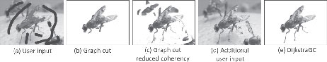
FIGURE 3.7
Illustrating the connectivity prior from [41]. (a) Image with user-scribbles (green, foreground; blue, background). Image segmentation using graph cut with standard (b) and reduced coherency (c). None of the results are perfect. By enforcing that the foreground object is 4-connected, a perfect result can be achieved (e). Note: this result is obtained by starting with the segmentation in (b) and then adding the 5 foreground user-clicks (red crosses) in (d).

where connectivity can, for instance, be defined on the standard 4-neighborhood grid. Apart from the connectivity constraint, the energy is a standard pairwise energy for segmentation, as in Equation (3.11). In [20] a modified version of this energy is solved with each user interaction. Consider the result in Figure 3.7(b) that is obtained with the input in 3.7(a). Given this result, the user places one red cross, e.g., at the tip of the fly’s leg (Figure 3.7(d)), to indicate another foreground pixel. The algorithm in [20] then has to solve the subproblem of finding a segmentation where both islands (body of the fly and red cross) are connected. For this a new method called DijkstraGC was developed, which combines the shortest-path Dijkstra algorithm and graph cut. In [20] it is also shown that for some practical instances DijkstraGC is globally optimal. It is worth commenting that the connectivity constraint enforces a different from of regularization compared to standard pairwise terms. Hence, in practice the strength of the pairwise terms may be chosen differently when the connectivity constraint potential is used.

The problem of minimizing the energy (3.18) directly has been addressed in Nowozin et al. [42], using a constraint-generation technique. They have shown that enforcing connectivity does help object recognition systems. Very recently the idea of connectivity was used for 3D reconstruction, i.e., to enforce that objects are connected in 3D, see details in [41].

Bounding Box Constraint

Building on the work [42], Lempitsky et al. [43] extended the connectivity constraint to the so-called bounding box prior. Figure 3.8 gives an example where the bounding box prior helps to achieve a good segmentation result.

The bounding box prior is formalized with the following energy

$\begin{array}{cc}E\left(x\right)={\displaystyle \sum _{i\in \mathcal{V}}{\psi }_i\left(x_i\right)}+{\displaystyle \sum _{\left(i,j\right)\in ℰ}{w}_{ij}\left|x_i-x_j\right|}& s.t.\forall C\in \Gamma {\displaystyle \sum _{i\in C}{x}_i\ge 1},\end{array}$

(3.19)

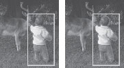
FIGURE 3.8
Bounding box prior. (Left) Typical result of the image segmentation method proposed in [29] where the user places the yellow bounding box around the object, which results in the blue segmentation. The result is expected since in the absence of additional prior knowledge the head of the person is more likely background, due to the dark colors outside the box. (Right) Improved result after applying the bounding box constraint. It enforces that the segmentation is spatially “close” to the four sides of the bounding box and also that the segmentation is connected.

where Γ is the set of all 4-connected “crossing” paths. A crossing path C is a path that goes from the top to the bottom side of the box, or from the left to the right side. Hence, the constraint in (3.19) forces that along each path C, there is at least one foreground pixel. This constraint makes sure that there exist a segmentation that touches all 4 sides of the bounding box and that is also 4-connected. As in [42], the problem is solved by first relaxing it to continuous labels, i.e., x_i ∈ [0, 1], and then applying a constraint-generation technique, where each constraint is a crossing path which violates the constraint in Equation (3.19). The resulting solution is then converted back to an integer solution, i.e., x_i ∈ {0, 1}, using a rounding schema called pin-pointing; see details in [43].

3.5.2    Constraints and Priors on Label Statistics

A simple and useful global potential is a cost based on the number of labels that are present in the final output. In its most simple form, the corresponding energy function has the form:

$E\left(x\right)={\displaystyle \sum _{i\in \mathcal{V}}{\psi }_i\left(x_i\right)}+{\displaystyle \sum _{\left(i,j\right)\in ℰ}{\psi }_{ij}\left(x_i,x_j\right)}+{\displaystyle \sum _{l\in L}{c}_l\left[\exists i:x_i=l\right]},$

(3.20)

where L is the set of all labels, c_l is the cost for each label, and [arg] is 1 if arg is true, and 0 otherwise. The above defined energy prefers a simpler solution over a more complex one.

The label cost potential has been used successfully in various domains, such as stereo [44], motion estimation [45], object segmentation [14], and object-instance recognition [46]. For instance, in [44] a 3D scene is reconstructed by a set of surfaces (planes or B-splines). A reconstruction with fewer surfaces is preferred due to the label-cost prior. One example where this prior helps is shown in Figure 3.9, where a plane, which is visible through a fence, is recovered as one plane instead of many planar fragments.

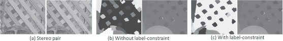
FIGURE 3.9
Illustrating the label-cost prior. (a) Crop of a stereo image (“cones” image from Middlebury database). (b) Result without a label-cost prior. In the left image each color represents a different surface, where gray-scale colors mark planes and nongrayscale colors, B-splines. The right image shows the resulting depth map. (c) Corresponding result with label-cost prior. The main improvement over (b) is that large parts of the green background (visible through the fence) are assigned to the same planar surface.

Various method have been proposed for minimizing the energy (3.20), including alpha-expansion (see details in [14, 45]). Extension to the energy defined in 3.20 have also been proposed. For instance, Ladicky et al. [14] have addressed the problem of minimizing energy functions containing a term whose cost is an arbitrary function of the set of labels present in the labeling.

Higher-Order Potentials Enforcing Label Counts

In many computer vision problems such as object segmentation or reconstruction, which are formulated in terms of labeling a set of pixels, we may know the number of pixels or voxels that can be assigned to a particular label. For instance, in the reconstruction problem, we may know the size of the object to be reconstructed. Such label count constraints are extremely powerful and have recently been shown to result in good solutions for many vision problems.

Werner [22] were one of the first to introduce constraints on label counts in energy minimization. They proposed a n-ary maxsum diffusion algorithm for solving these problems, and demonstrated its performance on the binary image denoising problem. Their algorithm, however, could only produce solutions for some label counts. It was not able to guarantee an output for any arbitrary label count desired by the user. Kolmogorov et al. [47] showed that for submodular energy functions, the parametric maxflow algorithm [48] can be used for energy minimization with label counting constraints. This algorithm outputs optimal solutions for only few label counts. Lim et al.[49] extended this work by developing a variant of the above algorithm they called decomposed parametric maxflow. Their algorithm is able to produce solutions corresponding to many more label counts.

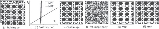
FIGURE 3.10
Illustrating the advantage of using an marginal probability field (MPF) over an MRF. (a) Set of training images for binary texture denoising. Superimposed is a pairwise term (translationally invariant with shift (15; 0); 3 exemplars in red). Consider the labeling k = (1, 1) of this pairwise term ϕ. Each training image has a certain number h_{(1, 1)} of (1, 1) labels, i.e. h_{(1, 1)} = Σ_i[ϕ_i = (1, 1)]. The negative logarithm of the statistics {h_{(1, 1)}} over all training images is illustrated in blue (b). It shows that all training images have roughly the same number of pairwise terms with label (1, 1). The MPF uses the convex function f_k (blue) as cost function. It is apparent that the linear cost function of an MRF is a bad fit. (c) A test image and (d) a noisy input image. The result with an MRF (e) is inferior to the MPF model (f). Here the MPF uses a global potential on unary and pairwise terms.

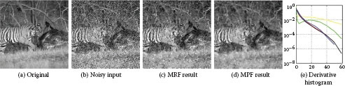
FIGURE 3.11
Results for image denoising using a pairwise MRF (c) and an MPF model (d). The MPF forces the derivatives of the solution to follow a mean distribution, which was derived from a large dataset. (f) Shows derivative histograms (discretized into the 11 bins). Here black is the target mean statistic, blue is for the original image (a), yellow for noisy input (b), green for the MRF result (c), and red for the MPF result (d). Note, the MPF result is visually superior and does also match the target distribution better. The runtime for the MRF (c) is 1096s and for MPF (d) 2446s.

Marginal Probability Fields

Finally, let us review the marginal probability field introduced in [50], which uses a global potential to overcome some fundamental limitations of maximum a posterior (MAP) estimation in Markov random fields (MRFs).

The prior model of a Markov random field suffers from a major drawback: the marginal statistics of the most likely solution (MAP) under the model generally do not match the marginal statistics used to create the model. Note, we refer to the marginal statistics of the cliques used in the model, which generally equates to those statistics deemed important. For instance, the marginal statistics of a single clique for a binary MRF are the number of 0s and 1s of the output labeling.

To give an example, given a corpus of binary training images that each contain 55% white and 45% black pixels (with no other significant statistic), a learned MRF prior will give each output pixel an independent probability of 0.55 of being white. Since the most likely value for each pixel is white, the most likely image under the model has 100% white pixels, which compares unfavorably with the input statistic of only 55%. When combined with data likelihoods, this model will therefore incorrectly bias the MAP solution towards being all white, the more so the greater the noise and hence data uncertainty.

The marginal probability field (MPF) overcomes this limitation. Formally, the MPF is defined as

$E\left(x\right)={\displaystyle \sum _k{f}_k}\left({\displaystyle \sum _i\left[{\varphi }_i\left(x\right)=k\right]}\right),$

(3.21)

where [arg] is defined as above, ϕ_i(x) returns the labeling of a factor at position i, k is an n-d vector, and f_k is the MPF cost kernel $ℝ\to {ℝ}^{+}$. For example, a pairwise factor of a binary random field has |k| = 4 possible states, i.e. k ∈ {(0, 0),(0, 1),(1, 0), (1, 1)}.

The key advantage of an MPF over an MRF is that the cost kernel f_k is arbitrary. In particular, by choosing a convex form for the kernel any arbitrary marginal statistics can be enforced. Figure 3.10 gives an example for binary texture denoising. Unfortunately, the underlying optimization problem is rather challenging, see details in [50]. Note that linear and concave kernels result in tractable optimization problems, e.g. for unary factors this has been described in Section 3.3.1 (see Figure 3.3(b) for a concave kernel for ${\displaystyle {\sum }_i\left[x_i=1\right]}$).

The MPF can be used in many applications, such as denoising, tracking, segmentation, and image synthesis (see [50]). Figure 3.11 illustrates an example for image denoising.

3.6    Maximum a Posteriori Inference

Given an MRF, the problem of estimating the maximum a posteriori (MAP) solution can be formulated as finding the labeling x that has the lowest energy. Formally, this procedure (also referred to as energy minimization) involves solving the following problem:

$x*=\arg \underset{x}{\min }E\left(x;d\right).$

(3.22)

The problem of minimizing a general energy function is NP-hard in general, and remains hard even if we restrict the arity of potentials to 2 (pairwise energy functions). A number of polynomial time algorithms have been proposed in the literature for minimizing pairwise energy functions. These algorithms are able to find either exact solutions for certain families of energy functions or approximate solutions for general functions. These approaches can broadly be classified into two categories: message passing and move making. Message passing algorithms attempt to minimize approximations of the free energy associated with the MRF [10, 51, 52].

Move making approaches refer to iterative algorithms that move from one labeling to the other while ensuring that the energy of the labeling never increases. The move space (that is, the search space for the new labeling) is restricted to a subspace of the original search space that can be explored efficiently [2]. Many of the above approaches (both message passing [10, 51, 52] and move making [2]) have been shown to be closely related to the standard LP relaxation for the pairwise energy minimization problem [53].

Although there has been work on applying message passing algorithms for minimizing certain classes of higher-order energy functions [21, 18], the general problem has been relatively ignored. Traditional methods for minimizing higher-order functions involve either (1) converting them to a pairwise form by addition of auxiliary variables, followed by minimization using one of the standard algorithms for pairwise functions (such as those mentioned above) [5, 38, 37, 26], or (2) using dual-decomposition which works by decomposing the energy functions into different parts, solving them independently, and then merging the solution of the different parts [20, 50].

3.6.1    Transformation-Based Methods

As mentioned before, any higher-order function can be converted to a pairwise one by introducing additional auxiliary random variables [5, 24]. This enables the use of conventional inference algorithms such as belief propagation, tree-reweighted message passing, and graph cuts for such models. However, this approach suffers from the problem of combinatorial explosion. Specifically, a naive transformation can result in an exponential number of auxiliary variables (in the size of the corresponding clique) even for higher-order potentials with special structure [38, 37, 26].

In order to avoid the undesirable scenario presented by the naive transformation, researchers have recently started focusing on higher-order potentials that afford efficient algorithms [25, 15, 22, 23, 50]. Most of the efforts in this direction have been towards identifying useful families of higher-order potentials and designing algorithms specific to them. While this approach has led to improved results, its long-term impact on the field is limited by the restrictions placed on the form of the potentials. To address this issue, some recent works [24, 14, 45, 38, 37, 26] have attempted to characterize the higher-order potentials that are amenable to optimization. These works have successfully been able to exploit the sparsity of potentials and provide a convenient parameterization of tractable potentials.

Transforming Higher-Order Pseudo-Boolean Functions

The problem of transforming a general submodular higher-order function to a second order one has been well studied. Kolmogorov and Zabih [3] showed that all submodular functions of order three can be transformed to one of order two, and thus can be solved using graph cuts. Freedman and Drineas [54] showed how certain submodular higher-order functions can be transformed to submodular second order functions. However, their method, in the worst case, needed to add an exponential number of auxiliary binary variables to make the energy function second order.

The special form of the Robust Pⁿ model (3.7) allows it to be transformed to a pairwise function with the addition of only two binary variables per higher-order potential. More formally, Kohli et al. [25] showed that higher-order pseudo-boolean functions of the form:

$f\left(x_c\right)=\min \left({\theta }_0+{\displaystyle \sum _{i\in c}{w}_i^0\left(1-x_i\right)},{\theta }_1+{\displaystyle \sum _{i\in c}{w}_i^1{x}_i},{\theta }_{\max }\right)$

(3.23)

can be transformed to submodular quadratic pseudo-boolean functions, and hence can be minimized using graph cuts. Here, x_i ∈ {0, 1} are binary random variables, c is a clique of random variables, x_c ∈ {0, 1}^|c| denotes the labelling of the variables involved in the clique, and $w_i^0\ge 0,w_i^1\ge 0,{\theta }_0,{\theta }_1,{\theta }_{\max }$ are parameters of the potential satisfying the constraints θ_max ≥ θ₀, θ₁, and

$\begin{array}{cc}\left(\left({\theta }_{\max }\le {\theta }_0+{\displaystyle \sum _{i\in c}{w}_i^0\left(1-x_i\right)}\right)\vee \left({\theta }_{\max }\le {\theta }_1+{\displaystyle \sum _{i\in c}{w}_i^1{x}_i}\right)\right)=1& \forall x\in {\left\{0,1\right\}}^{\left|c\right|}\end{array}$

(3.24)

where ∨ is a boolean OR operator. The transformation to a quadratic pseudo-boolean function requires the addition of only two binary auxiliary variables, making it computationally efficient.

Theorem The higher-order pseudo-boolean function

$f\left(x_c\right)=\min \left({\theta }_0+{\displaystyle \sum _{i\in c}{w}_i^0\left(1-x_i\right),{\theta }_1+{\displaystyle \sum _{i\in c}{w}_i^1{x}_i,{\theta }_{\max }}}\right)$

(3.25)

can be transformed to the submodular quadratic pseudo-boolean function

$f\left(x_c\right)=\underset{m_0,m_1}{\min }\left(r_0\left(1-m_0\right)+m_0{\displaystyle \sum _{i\in c}{w}_i^0\left(1-x_i\right)+r_1{m}_1+\left(1-m_1\right){\displaystyle \sum _{i\in c}{w}_i^1{x}_i-K}}\right)$

(3.26)

by the addition of binary auxiliary variables m₀ and m₁. Here, r₀ = θ_max − θ₀, r₁ = θ_max − θ₁ and K = θ_max − θ₀ − θ₁. (See proof in [55]).

Multiple higher-order potentials of the form (3.23) can be summed together to obtain higher-order potentials of the more general form

$f\left(x_c\right)=F_c\left({\displaystyle \sum _{i\in c}{x}_i}\right)$

(3.27)

where $F_c:ℝ\to ℝ$ is any concave function. However, if the function F_c is convex (as discussed in Section 3.4) then this transformation scheme does not apply. Kohli and Kumar [24] have shown how the minimization of energy function containing higher-order potentials of the form 3.27 with convex functions F_c can be transformed to a compact max-min problem. However, this problem is computationally hard and does not lend itself to conventional maxflow based algorithms.

Transforming Pattern-Based Higher-Order Potentials

We will now describe the method used in [26] to transform the minimization of an arbitrary higher-order potential functions to the minimization of an equivalent quadratic function. We start with a simple example to motivate our transformation.

Consider a higher-order potential function that assigns a cost θ₀ if the variables x_c take a particular labeling $X_0\in {ℒ}^{\left|c\right|}$, and θ₁ otherwise. More formally,

${\psi }_c\left(x_c\right)=\{\begin{array}{lll}{\theta }_0\hfill & \hfill \text{if}\hfill & x_c=X_0\hfill \\ {\theta }_1\hfill & \hfill \text{otherwise}.\hfill & \hfill \end{array}$

(3.28)

where θ₀ ≤ θ₁, and X₀ denotes a particular labeling of the variables x_c. The minimization of this higher-order function can be transformed to the minimization of a quadratic function using one additional switching variable z as:

$\underset{x_c}{\min }{\psi }_c\left(x_c\right)=\underset{x_c,z\in \left\{0,1\right\}}{\min }f\left(z\right)+{\displaystyle \sum _{i\in c}{g}_i\left(z,x_i\right)}$

(3.29)

where the selection function f is defined as: f(0) = θ₀ and f(1) = θ₁, while the consistency function g_i is defined as:

$g_i\left(z,x_i\right)=\{\begin{array}{ll}\hfill 0\hfill & \text{if}z=1\hfill \\ \hfill 0\hfill & \text{if}z=0\text{and}{x}_i=X_0\left(i\right)\hfill \\ \hfill \inf \hfill & \text{otherwise}.\hfill \end{array}$

(3.30)

where X₀(i) denotes the label of variable x_i in labeling X₀.

Transforming Pattern-Based Higher-Order Potentials with Deviations

The minimization of a pattern-based potential with deviation functions (as defined in Section 3.3.2) can be transformed to the minimization of a pairwise function using a (t + 1)-state switching variable as:

$\underset{x_c}{\min }{\psi }_c\left(x_c\right)=\underset{x_c,z\in \left\{1,2,\dots ,t+1\right\}}{\min }f\left(z\right)+{\displaystyle \sum _{i\in c}g\left(z,x_i\right)}$

(3.31)

$\begin{array}{cc}\text{where}& f\left(z\right)\end{array}=\{\begin{array}{ll}\hfill {\theta }_q\hfill & \text{if}z=q\in \left\{1,\dots ,t\right\}\hfill \\ \hfill {\theta }_{\max }\hfill & \text{if}z=t+1,\hfill \end{array}$

(3.32)

$g_i\left(z,x_i\right)=\{\begin{array}{lll}\hfill w_{il}^q\hfill & \text{if}\hfill & z=q\text{and}{x}_i=l\in ℒ\hfill \\ \hfill 0\hfill & \text{if}\hfill & z=t+1.\hfill \end{array}$

(3.33)

The role of the switching variable in the above mentioned transformation can be seen as that of finding which deviation function will assign the lowest cost to any particular labeling. The reader should observe that the last, i.e., (t + 1)^th state of the switching variable z does not penalize any labeling of the clique variables x_c. It should also be noted that the transformation method described above can be used to transform any general higher-order potential. However, in the worst case, the addition of a switching variable with ${\left|ℒ\right|}^{\left|c\right|}$ states is required, which makes minimization of even moderate order functions infeasible. Furthermore, in general the pairwise function resulting from this transformation is NP-hard.

3.6.2    Dual Decomposition

Dual decomposition has been successfully used for minimizing energy functions containing higher-order potentials. The approach works by decomposing the energy functions into different parts, solving them independently, and then merging the solution of the different parts. Since the merging step provides a lower bound on the original function, the process is repeated until the lower bound is optimal. For a particular task at hand the main question is on how to decompose the given problem into parts. This decomposition can have a major effect on the quality of the solution.

Let us explain the optimization procedure using the higher-order energy (3.15) for image segmentation. The function has the form

$E\left(x\right)=\underset{E^1\left(x\right)}{\underbrace{{\displaystyle \sum _k{h}_k\left(n_k^1\right)+{\displaystyle \sum _{\left(i,j\right)\in ℰ}{w}_{ij}\left|x_i-x_j\right|}}}}+\underset{E^2\left(x\right)}{\underbrace{h\left(n^1\right)}},$

(3.34)

where h_k(·) are concave functions and h(·) is a convex function. Recall that $n_k^1$ and n¹ are functions of the segmentation: $n_k^1={\displaystyle {\sum }_{i\in V_k}{x}_i}$ and $n^1={\displaystyle {\sum }_{i\in V}{x}_i}$. It can be seen that the energy function (3.34) is composed of a submodular part (E¹(x)) and a supermodular (E²(x)) part. As shown in [19] minimizing function (3.34) is an NP-hard problem.

We now apply the dual-decomposition technique to this problem. Let us rewrite the energy as

$E\left(x\right)=\left[E^1\left(x\right)-\langle y,x\rangle \right]+\left[E^2\left(x\right)+\langle y,x\rangle \right],$

(3.35)

where y is a vector in ${ℝ}^n$, n = |V|, and 〈y, x〉 denotes the dot product between two vectors. In other words, we added unary terms to one subproblem and subtracted them from the other one. This is a standard use of the dual-decomposition approach for MRF optimization [56]. Taking the minimum of each term in (3.35), over x gives a lower bound on E(x):

$\varphi \left(y\right)=\underset{{\varphi }^1\left(y\right)}{\underbrace{\underset{x}{\min }\left[E^1\left(x\right)-\langle y,x\rangle \right]}}+\underset{{\varphi }^2\left(y\right)}{\underbrace{\underset{x}{\min }\left[E^2\left(x\right)-\langle y,x\rangle \right]}}\le \underset{x}{\min }E\left(x\right).$

(3.36)

Note that both minima, i.e., for ϕ¹(y) and ϕ²(y), can be computed efficiently. In particular, the first term can be optimized via a reduction to an min s-t cut problem [25].

To get the tightest possible bound we need to maximize ϕ(y) over y. Function ϕ(·) is concave, therefore, one could use some standard concave maximization technique, such as a subgradient method, which is guaranteed to converge to an optimal bound. In [19] it is shown that in this case the tightest bound can be computed in polynomial time using a parametric maxflow technique [47].

3.7    Conclusions and Discussion

In this chapter we reviewed a number of higher-order models for computer vision problems. We showed how the ability of higher-order models to encode complex statistics between pixels makes them an ideal candidate for image labelling problems. The focus of the chapter has been on models based on discrete variables. It has not covered some families of higher-order models such as fields of experts [17] and product of experts [57] that have been shown to lead to excellent results for problem such as image denoising.

We also addressed the inherent difficulty in representing higher-order models and in performing inference in them. Learning of higher-order models involving discrete variables has seen relatively little work, and should attract more research in the future.

Another family of models that are able to encode complex relationships between pixels are hierarchical models which contain latent variables. Typical examples of such models include deep belief nets (DBN) and restricted boltzmann machines (RBM). There are a number of interesting relationships between these models and higher-order random fields [27]. We believe the investigation of these relationships is a promising direction for future work. We believe this would lead to better understanding of the modeling power of both families of models, as well as lead to new insights which may help in the development of better inference and learning techniques.

Bibliography

[1]  R. Szeliski, R. Zabih, D. Scharstein, O. Veksler, V. Kolmogorov, A. Agarwala, M. Tappen, and C. Rother, “A comparative study of energy minimization methods for Markov random fields.” in ECCV, 2006, pp. 16–29.

[2]  Y. Boykov, O. Veksler, and R. Zabih, “Fast approximate energy minimization via graph cuts.” PAMI, vol. 23, no. 11, pp. 1222–1239, 2001.

[3]  V. Kolmogorov and R. Zabih, “What energy functions can be minimized via graph cuts?.” PAMI, vol. 26, no. 2, pp. 147–159, 2004.

[4]  N. Komodakis, G. Tziritas, and N. Paragios, “Fast, approximately optimal solutions for single and dynamic MRFs,” in CVPR, 2007, pp. 1–8.

[5]  E. Boros and P. Hammer, “Pseudo-boolean optimization.” Discrete Appl. Math., vol. 123, no. 1-3, pp. 155–225, 2002.

[6]  E. Boros, P. Hammer, and G. Tavares, “Local search heuristics for quadratic unconstrained binary optimization (QUBO),” J. Heuristics, vol. 13, no. 2, pp. 99–132, 2007.

[7]  P. Felzenszwalb and D. Huttenlocher, “Efficient Belief Propagation for Early Vision,” in Proc. CVPR, vol. 1, 2004, pp. 261–268.

[8]  J. Pearl, “Fusion, propagation, and structuring in belief networks,” Artif. Intell., vol. 29, no. 3, pp. 241–288, 1986.

[9]  Y. Weiss and W. Freeman, “On the optimality of solutions of the max-product belief-propagation algorithm in arbitrary graphs.” Trans. Inf. Theory, 2001.

[10]  V. Kolmogorov, “Convergent tree-reweighted message passing for energy minimization.” IEEE Trans. Pattern Anal. Mach. Intell., vol. 28, no. 10, pp. 1568–1583, 2006.

[11]  M. Wainwright, T. Jaakkola, and A. Willsky, “Map estimation via agreement on trees: message-passing and linear programming.” IEEE Trans. Inf. Theory, vol. 51, no. 11, pp. 3697–3717, 2005.

[12]  N. Y. El-Zehiry and L. Grady, “Fast global optimization of curvature,” in CVPR, 2010, pp. 3257–3264.

[13]  A. Fitzgibbon, Y. Wexler, and A. Zisserman, “Image-based rendering using image-based priors.” in ICCV, 2003, pp. 1176–1183.

[14]  L. Ladicky, C. Russell, P. Kohli, and P. H. S. Torr, “Graph cut based inference with co-occurrence statistics,” in ECCV, 2010, pp. 239–253.

[15]  P. Kohli, M. Kumar, and P. Torr, “P3 and beyond: Solving energies with higher order cliques,” in CVPR, 2007.

[16]  X. Lan, S. Roth, D. Huttenlocher, and M. Black, “Efficient belief propagation with learned higher-order markov random fields.” in ECCV, 2006, pp. 269–282.

[17]  S. Roth and M. Black, “Fields of experts: A framework for learning image priors.” in CVPR, 2005, pp. 860–867.

[18]  B. Potetz, “Efficient belief propagation for vision using linear constraint nodes,” in CVPR, 2007.

[19]  S. Vicente, V. Kolmogorov, and C. Rother, “Joint optimization of segmentation and appearance models,” in ICCV, 2009, pp. 755–762.

[20]  ——, “Graph cut based image segmentation with connectivity priors,” in CVPR, 2008.

[21]  D. Tarlow, I. E. Givoni, and R. S. Zemel, “Hop-map: Efficient message passing with high order potentials,” JMLR - Proceedings Track, vol. 9, pp. 812–819, 2010.

[22]  T. Werner, “High-arity interactions, polyhedral relaxations, and cutting plane algorithm for soft constraint optimisation (MAP-MRF),” in CVPR, 2009.

[23]  O. Woodford, P. Torr, I. Reid, and A. Fitzgibbon, “Global stereo reconstruction under second order smoothness priors,” in CVPR, 2008.

[24]  P. Kohli and M. P. Kumar, “Energy minimization for linear envelope MRFs,” in CVPR, 2010, pp. 1863–1870.

[25]  P. Kohli, L. Ladicky, and P. Torr, “Robust higher order potentials for enforcing label consistency,” in CVPR, 2008.

[26]  C. Rother, P. Kohli, W. Feng, and J. Jia, “Minimizing sparse higher order energy functions of discrete variables,” in CVPR, 2009, pp. 1382–1389.

[27]  C. Russell, L. Ladicky, P. Kohli, and P. H. S. Torr, “Exact and approximate inference in associative hierarchical random fields using graph-cuts,” in UAI, 2010.

[28]  A. Blake, C. Rother, M. Brown, P. Perez, and P. Torr, “Interactive image segmentation using an adaptive GMMRF model,” in ECCV, 2004, pp. I: 428–441.

[29]  C. Rother, V. Kolmogorov, and A. Blake, “Grabcut: interactive foreground extraction using iterated graph cuts,” in SIGGRAPH, 2004, pp. 309–314.

[30]  A. Blake, P. Kohli, and C. Rother, Advances in Markov Random Fields. MIT Press, 2011.

[31]  S. Nowozin and C. Lampert, Structured Learning and Prediction in Computer Vision. NOW Publishers, 2011.

[32]  A. Shekhovtsov, P. Kohli, and C. Rother, “Curvature prior for MRF-based segmentation and shape inpainting,” Center for Machine Perception, K13133 FEE Czech Technical University, Prague, Czech Republic, Research Report CTU–CMP–2011–11, September 2011.

[33]  X. Ren and J. Malik, “Learning a classification model for segmentation.” in ICCV, 2003, pp. 10–17.

[34]  J. Shotton, J. Winn, C. Rother, and A. Criminisi, “TextonBoost: Joint appearance, shape and context modeling for multi-class object recognition and segmentation.” in ECCV (1), 2006, pp. 1–15.

[35]  D. Comaniciu and P. Meer, “Mean shift: A robust approach toward feature space analysis.” IEEE Trans. Pattern Anal. Mach. Intell., vol. 24, no. 5, pp. 603–619, 2002.

[36]  Y. Boykov and M. Jolly, “Interactive graph cuts for optimal boundary and region segmentation of objects in N-D images,” in ICCV, 2001, pp. I: 105–112.

[37]  N. Komodakis and N. Paragios, “Beyond pairwise energies: Efficient optimization for higher-order MRFs,” in CVPR, 2009, pp. 2985–2992.

[38]  H. Ishikawa, “Higher-order clique reduction in binary graph cut,” in CVPR, 2009, pp. 2993–3000.

[39]  W. T. Freeman, E. C. Pasztor, and O. T. Carmichael, “Learning low-level vision,” IJCV, vol. 40, no. 1, pp. 25–47, 2000.

[40]  D. Cremers and L. Grady, “Statistical priors for efficient combinatorial optimization via graph cuts,” in ECCV, 2006, pp. 263–274.

[41]  M. Bleyer, C. Rother, P. Kohli, D. Scharstein, and S. Sinha, “Object stereo: Joint stereo matching and object segmentation,” in CVPR, 2011, pp. 3081–3088.

[42]  S. Nowozin and C. H. Lampert, “Global connectivity potentials for random field models,” in CVPR, 2009, pp. 818–825.

[43]  V. S. Lempitsky, P. Kohli, C. Rother, and T. Sharp, “Image segmentation with a bounding box prior,” in ICCV, 2009, pp. 277–284.

[44]  M. Bleyer, C. Rother, and P. Kohli, “Surface stereo with soft segmentation,” in CVPR, 2010, pp. 1570–1577.

[45]  A. Delong, A. Osokin, H. N. Isack, and Y. Boykov, “Fast approximate energy minimization with label costs,” in CVPR, 2010, pp. 2173–2180.

[46]  D. Hoiem, C. Rother, and J. M. Winn, “3D layoutcrf for multi-view object class recognition and segmentation,” in CVPR, 2007.

[47]  V. Kolmogorov, Y. Boykov, and C. Rother, “Applications of parametric maxflow in computer vision,” in ICCV, 2007, pp. 1–8.

[48]  G. Gallo, M. Grigoriadis, and R. Tarjan, “A fast parametric maximum flow algorithm and applications,” SIAM J. on Comput., vol. 18, pp. 30–55, 1989.

[49]  Y. Lim, K. Jung, and P. Kohli, “Energy minimization under constraints on label counts,” in ECCV, 2010, pp. 535–551.

[50]  O. Woodford, C. Rother, and V. Kolmogorov, “A global perspective on map inference for low-level vision,” in ICCV, 2009, pp. 2319–2326.

[51]  D. Sontag, T. Meltzer, A. Globerson, T. Jaakkola, and Y. Weiss, “Tightening lp relaxations for map using message passing,” in UAI, 2008.

[52]  J. Yedidia, W. Freeman, and Y. Weiss, “Generalized belief propagation.” in NIPS, 2000, pp. 689–695.

[53]  C. Chekuri, S. Khanna, J. Naor, and L. Zosin, “A linear programming formulation and approximation algorithms for the metric labeling problem,” SIAM J. Discrete Math., vol. 18, no. 3, pp. 608–625, 2005.

[54]  D. Freedman and P. Drineas, “Energy minimization via graph cuts: Settling what is possible.” in CVPR, 2005, pp. 939–946.

[55]  P. Kohli, L. Ladicky, and P. H. S. Torr, “Robust higher order potentials for enforcing label consistency,” IJCV, vol. 82, no. 3, pp. 302–324, 2009.

[56]  L. Torresani, V. Kolmogorov, and C. Rother, “Feature correspondence via graph matching: Models and global optimization,” in ECCV, 2008, pp. 596–609.

[57]  G. E. Hinton, “Training products of experts by minimizing contrastive divergence,” Neural Comput., vol. 14, no. 8, pp. 1771–1800, 2002.

¹Potentials defined over all variables in the problem are referred to as global potentials.

²Representation of a general m order potential function of k-state discrete variables requires k^m parameter values

³El-Zehiry and Grady [12] used potentials defined over 2 × 2 patches to enforce smoothness. Shekhovtsov et al. [32] have recently proposed a higher order model for encouraging smooth, low curvature image segmentations that uses potentials defined over much large sets of variables and was learnt using training data.

⁴Kohli et al. ignore a part of the TextonBoost [34] energy that represents a global appearance model for each object-class. In Section 3.4 we will revisit this issue and show that in fact this global, appearance model is closely related to the higher-order potentials defined in [25].

⁵For the problem of [25], this is the number of pixels constituting super-pixel c.