1

Graph theory concepts and definitions used in image processing and analysis

Olivier Lézoray

Université de Caen Basse-Normandie
GREYC UMR CNRS 6072
6 Bvd. Maréchal Juin
F-14050 CAEN, FRANCE

Email: [email protected]

Leo Grady

Department of Image Analytics and Informatics
Siemens Corporate Research
755 College Rd.
Princeton, NJ 08540, USA

Email: [email protected]

CONTENTS

1.1    Introduction

1.2    Basic Graph Theory

1.3    Graph Representation

1.3.1    Matrix Representations

1.3.2    Adjacency Lists

1.4    Paths, Trees, and Connectivity

1.4.1    Walks and Paths

1.4.2    Connected Graphs

1.4.3    Shortest Paths

1.4.4    Trees and Minimum Spanning Trees

1.4.5    Maximum Flows and Minimum Cuts

1.5    Graph Models in Image Processing and Analysis

1.5.1    The Regular Lattice

1.5.2    Irregular tessellations

1.5.3    Proximity Graphs for Unorganized Embedded Data

1.6    Conclusion

Bibliography

1.1    Introduction

Graphs are structures that have a long history in mathematics and have been applied in almost every scientific and engineering field (see [1] for mathematical history, and [2, 3, 4] for popular accounts). Many excellent primers on the mathematics of graph theory may be found in the literature [5, 6, 7, 8, 9, 10], and we encourage the reader to learn the basic mathematics of graph theory from these sources. We have two goals for this chapter: First, we make this work self-contained by reviewing the basic concepts and notations for graph theory that are used throughout this book. Second, we connect these concepts to image processing and analysis from a conceptual level and discuss implementation details.

1.2    Basic Graph Theory

Intuitively, a graph represents a set of elements and a set of pairwise relationships between those elements. The elements are called nodes or vertices, and the relationships are called edges. Formally, a graph GG$\mathcal{G}$ is defined by the sets $\mathcal{G}=\left(\mathcal{V},ℰ\right)$ in which $ℰ\subseteq \mathcal{V}\times \mathcal{V}$. We may denote the i-th vertex as ${\upsilon }_i\in \mathcal{V}$, and the i-th edge as $e_i\in ℰ$. Since each edge is a subset of two vertices, we may also write e_ij = {υ_i, υ_j}. In this book we do not consider graphs with self-loops, meaning that $e_{ij}\in ℰ$ implies that i ≠ j. We also do not consider graphs for which there are multiple edges of the same orientation connecting the same node pair. However, for specific graph encodings, self-loops and multiple edges can be useful (see Chapter 11).

Every graph may be viewed as weighted. Given a graph $\mathcal{G}=\left(\mathcal{V},ℰ\right)$, vertex weighting is a function $\widehat{w}:\mathcal{V}\to ℝ$, and edge weighting is a function $w:ℰ\to ℝ$. To simplify the notation, we will use w to refer to both vertex and edge weighting. The weight of a vertex is denoted by w(υ_i) or w_i, and the weight of an edge incident to two vertices is denoted by w(υ_i,υ_j) or w_ij. If w_i = 1, $\forall {\upsilon }_i\in \mathcal{V}$ and w_ij = 1, $\forall e_{ij}\in ℰ$, then we may consider the graph to be unweighted. If not otherwise specified, all node and edge weights are considered to be equal to unity. We treat w_ij = 0 as equivalent to $e_{ij}\notin ℰ$. Intuitively, an edge weight of zero is equivalent to meaning that the edge is not a member of the edge set.

Each edge is considered to be oriented and some edges additionally directed. An orientation of an edge means that each edge $e_{ij}\in ℰ$ contains an ordering of the vertices, υ_i and υ_j. An edge e_ij is directed if w_ij ≠ w_ij. A graph for which none of the edges are directed is called an undirected graph, and a graph in which at least one edge is directed is called a directed graph or digraph. A directed edge is represented by the notation e_i→j. A directed graph is more general than an undirected graph because it does not require that w_ij = w_ji for each edge. Consequently, all algorithms for directed graphs may also be applied to undirected graphs, but the converse may or may not be true. Therefore, in this chapter we use digraphs to illustrate the most general concepts.

The edge orientation of an undirected graph provides a reference to determine the sign of a flow through that edge. This concept was developed early in the circuit theory literature to describe the direction of current flow through a resistive branch (an edge). For example, a current flow through e_ij from node υ_i to υ_j is considered positive, while a current flow from υ_j to υ_i is considered negative. In this sense, flow through a directed edge is usually constrained to be strictly positive.

Drawing a graph is typically done by depicting each node with a circle and each edge with a line connecting circles representing the two nodes. The edge orientation or direction is usually represented by an arrow. Edge e_ij is drawn with an arrow pointing from node υ_i to node υ_j.

We consider two functions $s,t:ℰ\to \mathcal{V}$. Function s is called the source function, and function t is called the target function. Given an edge $e_{ij}=\left({\upsilon }_i,{\upsilon }_j\right)\in ℰ$, we say that s(e_ij) = υ_i is the origin or source of e_ij, and t(e_ij) = υ_j is the endpoint or target of e_ij. Given any edge, $e_k\in ℰ$, the vertices s(e_k) and t(e_k) are called the boundaries of e_k, and the expression t(e_k) − s(e_k) is called the boundary of e_k.

Given these preliminaries, we may now list a series of basic definitions:

1.  Adjacent: Two nodes υ_i and υ_j are called adjacent if $\exists e_{ij}\in ℰ$ or $\exists e_{ji}\in ℰ$, which is denoted by υ_i ~ υ_j. Two edges e_ij and e_sk are adjacent if they share a common vertex, that is, if i = s, i = k, j = s, or j = k.

2.  Incident: An edge e_ij is incident to nodes υ_i and υ_j (and each node is incident to the edge).

3.  Isolated: A node υ_i is called isolated if w_ij = w_ji = 0, $\forall {\upsilon }_j\in \mathcal{V}$. Intuitively, a node is isolated if it is not connected to the graph by an edge (of nonzero weight).

4.  Degree: The outer degree of node υ_i, deg⁻ (υ_i), is equal to ${\mathrm{deg}}^{-}\left({\upsilon }_i\right)={\displaystyle {\sum }_{e_{ij}\in ℰ}{w}_{ij}}$. The inner degree of node υ_i, deg⁺ (υ_i), is equal to ${\mathrm{deg}}^{+}\left({\upsilon }_i\right)={\displaystyle {\sum }_{e_{ji}\in ℰ}{w}_{ji}}$. Note that, in an undirected graph, deg⁻ (υ_i) = deg⁺ (υ_i), $\forall {\upsilon }_i\in \mathcal{V}$. Consequently, we may simply use d(υ_i) or d_i to denote the degree of a vertex in an undirected graph. An isolated node υ_i has zero degree.

5.  Complement: A graph $\overline{\mathcal{G}}=\left(\mathcal{V},\overline{ℰ}\right)$ is called the complement to graph $\mathcal{G}=\left(\mathcal{V},ℰ\right)$ if $\overline{ℰ}=\mathcal{V}\times \mathcal{V}-ℰ$. Therefore, the complement graph has all the same nodes as the original, but each node pair in the complement is connected iff the node pair was not connected in the original graph.

6.  Regular: An undirected graph is called regular if d_i = k, $\forall {\upsilon }_i\in \mathcal{V}$ for some constant k.

7.  Complete (fully connected): An undirected graph is called complete or fully connected if each node is connected to every other node by an edge, that is when $ℰ=\mathcal{V}\times \mathcal{V}$. A complete graph of n vertices is denoted K_n. Figure 1.1 gives an example of K₅.

8.  Partial graph: A graph ${\mathcal{G}}^{\prime }=\left(\mathcal{V},{ℰ}^{\prime }\right)$ is called a partial graph [11] of $\mathcal{G}=\left(\mathcal{V},ℰ\right)$ if ${ℰ}^{\prime }\subseteq ℰ$.

9.  Subgraph: A graph ${\mathcal{G}}^{\prime }=\left({\mathcal{V}}^{\prime },{ℰ}^{\prime }\right)$ is called a subgraph of $\mathcal{G}=\left(\mathcal{V},ℰ\right)$ if ${\mathcal{V}}^{\prime }\subseteq \mathcal{V}$, and ${ℰ}^{\prime }=\left\{e_{ij}\in ℰ|{\upsilon }_i\in {\mathcal{V}}^{\prime }\text{and}{\upsilon }_j\in {\mathcal{V}}^{\prime }\right\}$.

10.  clique: A clique is defined as a fully connected subset of the vertex set (see Figure 1.2).

11.  Bipartite: A graph is called bipartite if $\mathcal{V}$ can be partitioned into two subsets ${\mathcal{V}}_1\subset \mathcal{V}$ and ${\mathcal{V}}_2\subset \mathcal{V}$, where ${\mathcal{V}}_1\cap {\mathcal{V}}_2=\cancel{0}$ and ${\mathcal{V}}_1\cup {\mathcal{V}}_2=\mathcal{V}$, such that $ℰ\subseteq {\mathcal{V}}_1\times \mathcal{V}{}_2$. If $\left|\mathcal{V}\right|=m$ and $\left|\mathcal{V}\right|=n$, and $ℰ={\mathcal{V}}_1\times {\mathcal{V}}_2$, then $\mathcal{G}$ is called a complete bipartite graph and is denoted by K_m,n. Figure 1.2 gives an example of K_{3, 5}.

12.  Graph isomorphism: Let ${\mathcal{G}}_1=\left({\mathcal{V}}_1,{ℰ}_1\right)$ and ${\mathcal{G}}_2=\left({\mathcal{V}}_2,{ℰ}_2\right)$ be two undirected graphs. A bijection $f:{\mathcal{V}}_1\to {\mathcal{V}}_2$ from ${\mathcal{G}}_1$ to ${\mathcal{G}}_2$ is called a graph isomorphism if $\left({\upsilon }_i,{\upsilon }_j\right)\in {ℰ}_1$ implies that $\left(f\left({\upsilon }_i\right),f\left({\upsilon }_j\right)\right)\in {ℰ}_2$. Figure 1.3 shows an example of an isomorphism between two graphs.

13.  Higher-order graphs (hypergraph): A graph $G=\left(\mathcal{V},ℰ,ℱ\right)$ is considered to be a higher-order graph or hypergraph if each element of $ℱ,f_i\in ℱ$ is defined as a set of nodes for which each |f_i| > 2. Each element of a higher-order set is called a hyperedge, and each hyperedge may also be weighted. A k-uniform hypergraph is one for which all hyperedges have size k. Therefore, a 3-uniform hypergraph would be a collection of node triplets.

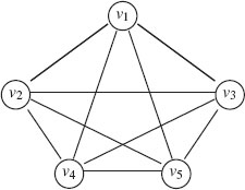
FIGURE 1.1
An example of complete graph K₅.

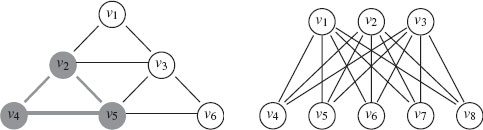
FIGURE 1.2
Left: A clique in a graph (grey). Right: The complete bipartite graph K_{3, 5} with ${\mathcal{V}}_1=\left\{{\upsilon }_1,{\upsilon }_2,{\upsilon }_3\right\}$ and ${\mathcal{V}}_2=\left\{{\upsilon }_4,{\upsilon }_5,{\upsilon }_6,{\upsilon }_7,{\upsilon }_8\right\}$.

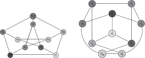
FIGURE 1.3
Example of two isomorphic graphs under the mapping ${\upsilon }_{10}\to {{\upsilon }^{\prime }}_3,{\upsilon }_9\to {{\upsilon }^{\prime }}_5,{\upsilon }_8\to {{\upsilon }^{\prime }}_2,{\upsilon }_7\to {{\upsilon }^{\prime }}_7,{\upsilon }_6\to {{\upsilon }^{\prime }}_8,{\upsilon }_5\to {{\upsilon }^{\prime }}_1,{\upsilon }_4\to {{\upsilon }^{\prime }}_{10},{\upsilon }_3\to {{\upsilon }^{\prime }}_4,{\upsilon }_2\to {{\upsilon }^{\prime }}_6,{\upsilon }_1\to {{\upsilon }^{\prime }}_9$.

1.3    Graph Representation

Several computer representations of graphs can be considered. The data structures used to represent graphs can have a significant influence on the size of problems that can be performed on a computer and the speed with which they can be solved. It is therefore important to know the different representations of graphs. To illustrate them, we will use the graph depicted in Figure 1.4.

1.3.1    Matrix Representations

A graph may be represented by one of several different common matrices. A matrix representation may provide efficient storage (since most graphs used in image processing are sparse), but each matrix representation may also be viewed as an operator that acts on functions associated with the nodes or edges of a graph.

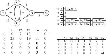
FIGURE 1.4
From top-left to bottom-right: a weighted directed graph, its adjacency list, its adjacency matrix, and its (transposed) incidence matrix representations.

The first matrix representation of a graph is given by the incidence matrix. The incidence matrix for $\mathcal{G}=\left(\mathcal{V},ℰ\right)$ is an $\left|ℰ\right|\times \left|\mathcal{V}\right|$ matrix A where

$A_{ij}=\{\begin{array}{c}-1\text{if}s\left(e_i\right)={\upsilon }_j,\\ +1\text{if}t\left(e_i\right)={\upsilon }_j,\\ 0\text{otherwise}.\end{array}$

(1.1)

The incidence matrix has the unique property of the matrices in this section that it preserves the orientation information of each edge but not the edge weight. The adjoint (transpose) of the incidence matrix also represents the boundary operator for a graph in the sense that multiplying this matrix with a signed indicator vector of edges in a path will return the endpoints of the path. Furthermore, the incidence matrix defines the exterior derivative for functions associated with the nodes of the graph. As such, this matrix plays a central role in discrete calculus (see [12] for more details).

The constitutive matrix of graph $\mathcal{G}=\left(\mathcal{V},ℰ\right)$ is an $\left|ℰ\right|\times \left|ℰ\right|$ matrix C where

$C_{ij}=\{\begin{array}{l}w\left(e_i\right)\text{if}i=j,\hfill \\ 0\text{otherwise}.\hfill \end{array}$

(1.2)

The adjacency matrix representation of graph $\mathcal{G}=\left(\mathcal{V},ℰ\right)$ is a $\left|\mathcal{V}\right|\times \left|\mathcal{V}\right|$ matrix W where

$W_{ij}=\{\begin{array}{l}{w}_{ij}\text{if}{e}_{ij}\in ℰ,\hfill \\ \text{0}\text{otherwise}.\hfill \end{array}$

(1.3)

For undirected graphs the matrix W is symmetric.

The Laplacian matrix of an undirected graph $\mathcal{G}=\left(\mathcal{V},ℰ\right)$ is a $\left|\mathcal{V}\right|\times \left|\mathcal{V}\right|$ matrix GL where

$L_{ij}=\{\begin{array}{c}{d}_i\text{if}i=j,\\ -w_{ij}\text{if}{e}_{ij}\in ℰ,\\ 0\text{otherwise},\end{array}$

(1.4)

and G is a diagonal matrix with G_ii = w(υ_i). In the context of the Laplacian matrix, w(υ_i) = 1 or $w\left({\upsilon }_i\right)=\frac{1}{d_i}$ are most often adopted (see [12] for a longer discussion on this point).

If G = I, then for an undirected graph these matrices are related to each other by the formula

$A^{T}CA=W-\mathcal{D}=L,$

(1.5)

where D is a diagonal matrix of node degrees with D_ii = d_i.

1.3.2    Adjacency Lists

The advantage of adjacency lists over matrix representations is less memory usage. Indeed, a full incidence matrix requires $O\left(\left|\mathcal{V}\right|\times \left|ℰ\right|\right)$ memory, and a full adjacency matrix requires $O\left({\left|\mathcal{V}\right|}^2\right)$ memory. However, sparse graphs can take advantage of sparse matrix representations for a much more efficient storage.

An adjacency list representation of a graph is an array L of $\left|\mathcal{V}\right|$ linked lists (one for each vertex of $\mathcal{V}$). For each vertex υ_i, there is a pointer L_i to a linked list containing all vertices υ_j adjacent to υ_i. For weighted graphs, the linked list contains both the target vertex and the edge weight. With this representation, iterating through the set of edges is $O\left(\left|\mathcal{V}\right|+\left|ℰ\right|\right)$ whereas it is $O\left({\left|\mathcal{V}\right|}^2\right)$ for adjacency matrices. However, checking if an edge $e_k\in ℰ$ is an $O\left(\left|\mathcal{V}\right|\right)$ operation with adjacency lists whereas it is an O(1) operation with adjacency matrices.

1.4    Paths, Trees, and Connectivity

Graphs model relationships between nodes. These relationships make it possible to define whether two nodes are connected by a series of pairwise relationships. This concept of connectivity, and the related ideas of paths and trees, appear in some form throughout this work. Therefore, we now review the concepts related to connectivity and the basic algorithms used to probe connectivity relationships.

1.4.1    Walks and Paths

Given a directed graph $\mathcal{G}=\left(\mathcal{V},ℰ\right)$ and two vertices ${\upsilon }_i,{\upsilon }_j\in \mathcal{V}$, a walk (also called a chain) from υ_i to υ_j is a sequence π(υ₁, υ_n) = (υ₁, e₁, υ₂, …, υ_n−1, e_n−1, υ_n), where n ≥ 1, ${\upsilon }_i\in \mathcal{V}$, and $e_j\in ℰ$:

${\upsilon }_1={\upsilon }_i,{\upsilon }_j={\upsilon }_n,\text{and}\left\{s\left(e_i\right),t\left(e_i\right)\right\}=\left\{{\upsilon }_i,{\upsilon }_{i+1}\right\},1\le i\le n.$

(1.6)

The length of the walk is denoted as |π| = n. A walk may contain a vertex or edge more than once. If υ_i = υ_j, the walk is called a closed walk; otherwise it is an open walk. A walk is called a trail if every edge is traversed only once. A closed trail is called a circuit. A circuit is called a cycle if all nodes are distinct. An open walk is a path if every vertex is distinct. A subpath is any sequential subset of a path. Figure 1.5 is used to illustrate the concepts of walk, trail, and path. In Figure 1.5, bolded grey arrows provide a walk π(υ₁, υ₁) = (υ₁, e₈, υ₅, e₇, υ₁, e₁, υ₂, e₆, υ₆, e₄, υ₅, e₇, υ₁) that is a closed walk, but is neither a trail (e₇ is traversed twice) nor a cycle. Dashed grey arrows provide a walk π(υ₆, υ₄) = (υ₆, e₅, υ₂, e₂, υ₃, e₃, υ₄) that is an open walk, a trail, and a path. Black arrows are arrows not involved in the walks π(υ₁, υ₁) and π(υ₆, υ₄).

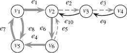
FIGURE 1.5
Illustration of a walk π(υ₁, υ₁) (bolded grey), trail, and path π(υ₆, υ₄) (dashed grey).

1.4.2    Connected Graphs

Two nodes are called connected if ∃π(υ_i, υ_j) or ∃π(υ_j, υ_i). A graph $\mathcal{G}=\left(\mathcal{V},ℰ\right)$ is called a connected graph iff $\forall {\upsilon }_i,{\upsilon }_j\in \mathcal{V},\exists \pi \left({\upsilon }_i,{\upsilon }_j\right)$, or ∃π(υ_j, υ_i). Therefore, the relation

${\upsilon }_i{R}_w{\upsilon }_j=\{\begin{array}{r}\hfill {\upsilon }_i={\upsilon }_j,\\ \hfill \exists \pi \left({\upsilon }_i,{\upsilon }_j\right)\text{or}\exists \pi \left({\upsilon }_j,{\upsilon }_i\right),\end{array}$

(1.7)

is an equivalence relation. The induced equivalence classes by this relation form a partition of $\mathcal{V}$ into ${\mathcal{V}}_1,{\mathcal{V}}_2,\dots ,{\mathcal{V}}_p$ subsets. Subgraphs ${\mathcal{G}}_1,{\mathcal{G}}_2,\dots ,{\mathcal{G}}_p$ induced by ${\mathcal{V}}_1,{\mathcal{V}}_2,\dots ,{\mathcal{V}}_p$ are called the connected components of the graph $\mathcal{G}$. Each connected component is a connected graph. The connected components of a graph $\mathcal{G}$ are the set of largest subgraphs of $\mathcal{G}$ that are each connected.

Two nodes are strongly connected if ∃π(υ_i, υ_j) and ∃π(υ_j, υ_i). If two nodes are connected but not strongly connected, then the nodes are called weakly connected. Note that, in an undirected graph, all connected nodes are strongly connected. The graph is strongly connected iff $\forall {\upsilon }_i,{\upsilon }_j\in \mathcal{V},\exists \pi \left({\upsilon }_i,{\upsilon }_j\right)$, and ∃π(υ_j, υ_i). Therefore, the relation

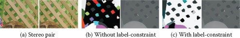
FIGURE 3.9
Illustrating the label-cost prior. (a) Crop of a stereo image (“cones” image from Middlebury database). (b) Result without a label-cost prior. In the left image each color represents a different surface, where gray-scale colors mark planes and nongrayscale colors, B-splines. The right image shows the resulting depth map. (c) Corresponding result with label-cost prior. The main improvement over (b) is that large parts of the green background (visible through the fence) are assigned to the same planar surface.

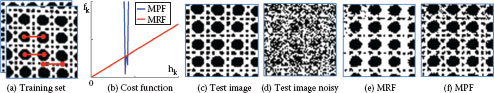
FIGURE 3.10
Illustrating the advantage of using an marginal probability field (MPF) over an MRF. (a) Set of training images for binary texture denoising. Superimposed is a pairwise term (translationally invariant with shift (15; 0); 3 exemplars in red). Consider the labeling k = (1, 1) of this pairwise term ϕ. Each training image has a certain number h_{(1, 1)} of (1, 1) labels, i.e. h_{(1, 1)} = Σ_i[ϕ_i = (1, 1)]. The negative logarithm of the statistics {h_{(1, 1)}} over all training images is illustrated in blue (b). It shows that all training images have roughly the same number of pairwise terms with label (1, 1). The MPF uses the convex function f_k (blue) as cost function. It is apparent that the linear cost function of an MRF is a bad fit. (c) A test image and (d) a noisy input image. The result with an MRF (e) is inferior to the MPF model (f). Here the MPF uses a global potential on unary and pairwise terms.

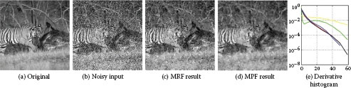
FIGURE 3.11
Results for image denoising using a pairwise MRF (c) and an MPF model (d). The MPF forces the derivatives of the solution to follow a mean distribution, which was derived from a large dataset. (f) Shows derivative histograms (discretized into the 11 bins). Here black is the target mean statistic, blue is for the original image (a), yellow for noisy input (b), green for the MRF result (c), and red for the MPF result (d). Note, the MPF result is visually superior and does also match the target distribution better. The runtime for the MRF (c) is 1096s and for MPF (d) 2446s.

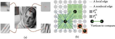
FIGURE 7.2
(a) Four examples of image patches. Central pixels (in red) are associated with vectors of gray-scale values within a patch of size 13 × 13 $\left(F_6^{f^0}\right)$. (b) Graph topology and feature vector illustration: a 8-adjacency grid graphs is constructed. The vertex surrounded by a red box shows the use of the simplest feature vector, i.e., the initial function. The vertex surrounded by a green box shows the use of a feature vector that exploits patches.

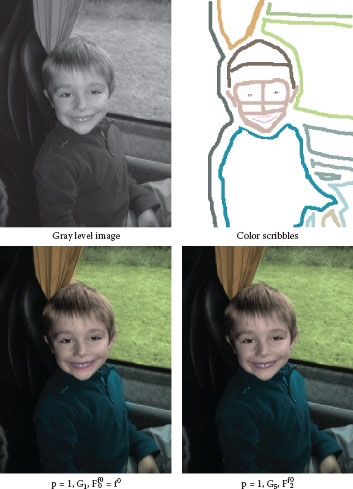
FIGURE 7.9
Isotropic colorization of a grayscale image with w = g₂ and λ = 0.01 in local and nonlocal configurations.

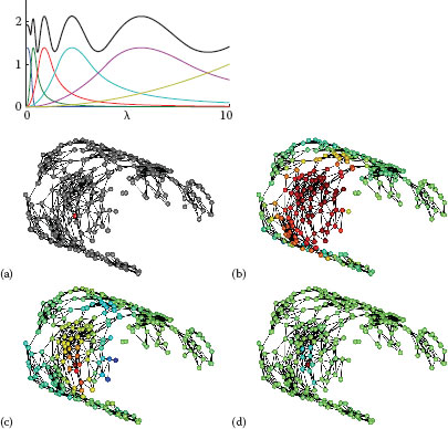
FIGURE 8.1
Left: Scaling function h(λ) (blue curve), wavelet generating kernels g(t_jλ), and sum of squares G (black curve), for J = 5 scales, λ_max = 10, K_1p = 20. Details in Section 8.2.3. Right: Example graph showing specified center vertex (a), scaling function (b) and wavelets at two scales (c,d). Figures adapted from [1].

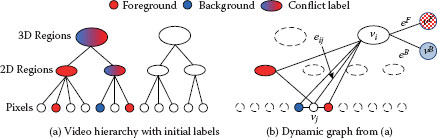
FIGURE 9.8
Video hierarchy and dynamic graph construction in the 3D video cutout system [38]. (a). Video hierarchy created by two-step mean shift segmentation. User-specified labels are then propagated upward from the bottom level. (b). A graph is dynamically constructed based on the current configuration of the labels. Only highest level nodes that have no conflict are selected. Each node in the hierarchy also connects to two virtual nodes υ^F and υ^B.

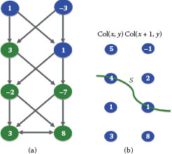
FIGURE 10.5
Illustrating the recovery of a feasible surface from a closed set. (a) shows a closed set in the constructed graph in Figure 10.4(d), which consists of all green nodes. The surface specified by the closed set in (a) is shown in (b).

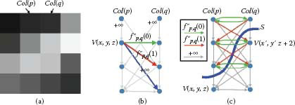
FIGURE 10.9
Graph construction for the convex smoothness penalty function. (a) Example of two adjacent columns. The smoothness parameter Δ_x = 2. (b) Weighted arcs introduced for each node V(x, y, z). Gray arcs of weight +∞ reflect the hard smoothness constraints. (c) Weighted arcs are built between nodes corresponding to the two adjacent columns. The feasible surface S cuts the arcs with a total weight of $f_{p,q}\left(2\right)=f_{p,q}^{″}\left(0\right)+\left[f_{p,q}^{″}\left(0\right)+f_{p,q}^{″}\left(1\right)\right]$, which determines smoothness shape compliance term of α(S) for the two adjacent columns.

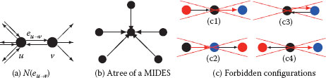
FIGURE 11.11
Directed neighborhood $\mathcal{N}\left(e_{u\to \upsilon }\right)$ of edge e_u→υ(a). A tree of a MIDES defining unambiguously its surviving vertex (b). Two edges within a same neighborhood cannot be both selected. Hence, red edges in (c) cannot be selected once black edges have been added to the MIDES.

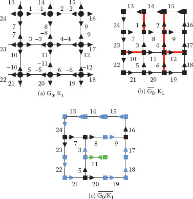
FIGURE 11.21
A combinatorial map (a) and its dual (b) encoding a 3 × 3 grid with the contraction kernel K₁ = α*(1, 2, 4, 12, 6, 10) (▬) superimposed to both figures. Only positive darts are represented in (b) and (c) in order to not overload them. The resulting reduced dual combinatorial map (c) should be further simplified by a removal kernel of empty self-loops (RKESL) K₂ = α*(11) to remove dual vertices of degree 1 (■). Dual vertices of degree 2 (■) are removed by the RKEDE K₃ = φ*(24, 13, 14, 15, 9, 22, 17, 21, 19, 18,) ∪ {3, −5}. Note that the dual vertex φ*(3) = (3, −5, 11) becomes a degree 2 vertex only after the removal of α*(11).

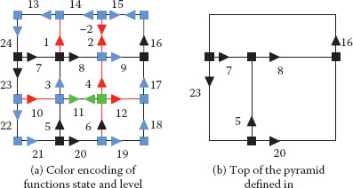
FIGURE 11.22
Implicit encoding (a) and top level combinatorial map (b) of the pyramid defined in Figure 11.21. Red, green and blue darts have level equal to 1, 2, and 3 respectively. States associated to these levels are, respectively, equal to CK, RKESL, RKEDE.

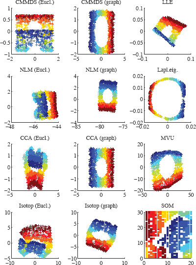
FIGURE 12.03
Two-dimensional embeddings of the Swiss roll with various NLDR methods. Distance-based methods use either Euclidean norm (‘Eucl.’) or shortest paths in a neighborhood graph (‘Graph’).

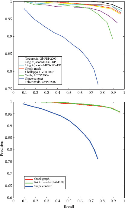
FIGURE 14.6
The recognition performance of the shock-graph matching based on the approach described above for the Kimia-99 and Kimia-216 shape databases [11].

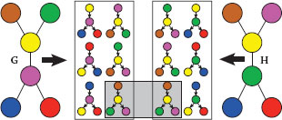
FIGURE 17.3
Graph kernels between two graphs (each color represents a different label). We display all binary 1-tree walks with a specific tree structure, extracted from two simple graphs. The graph kernels are computing and summing the local kernels between all those extracted tree-walks. In the case of the Dirac kernel (hard matching), only one pair of tree-walks is matched (for both labels and structures).

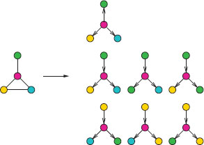
FIGURE 17.5
Examples of tree-walks from a graph. Each color represents a different label.

${\upsilon }_i{R}_s{\upsilon }_j=\{\begin{array}{r}\hfill {\upsilon }_i={\upsilon }_j\\ \hfill \exists \pi \left({\upsilon }_i,{\upsilon }_j\right)\text{and}\exists \pi \left({\upsilon }_j,{\upsilon }_i\right),\end{array}$

(1.8)

is an equivalence relation. The subgraphs induced by the obtained partition of $\mathcal{G}$ are the strongly connected components of $\mathcal{G}$. Figure 1.6 illustrates the concepts of strongly and weakly connected components.

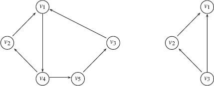
FIGURE 1.6
Left: A strongly connected component. Right: A weakly connected component.

1.4.3    Shortest Paths

The problems of routing in graphs (in particular the search for a shortest path) are among the oldest and most common problems in graph theory. Let $\mathcal{G}=\left(\mathcal{V},ℰ\right)$ be a weighted graph where a weight function $w:ℰ\to ℝ$ associates a real value (i.e., a weight also called a length in this context) to each edge.¹ In this section we consider only graphs for which all edge weights are nonnegative. Let l(π(υ_i, υ_j)) denote the total weight (or length) of a walk:

$l\left(\pi \left({\upsilon }_i,{\upsilon }_j\right)\right)={\displaystyle \sum _{e_k\in \pi \left({\upsilon }_i,{\upsilon }_j\right)}w\left(e_k\right)}.$

(1.9)

We will also use the convention that the length of the walk equals ∞ if υ_i and υ_j are not connected and l(π(υ_i, υ_i)) = 0. The minimum length between two vertices is

$l*\left({\upsilon }_i,{\upsilon }_j\right)=\underset{\pi \left({\upsilon }_i,{\upsilon }_j\right)}{\arg \min }l\left(\pi \left({\upsilon }_i,{\upsilon }_j\right)\right).$

(1.10)

A walk satisfying the minimum in (1.10) is a path called a shortest path. The shortest path between two nodes may not be unique. Different algorithms can be used to compute l* if one wants to find a shortest path from one vertex to all the others or between all pairs of vertices. We will restrict ourselves to the first kind of problem.

To compute the shortest path from one vertex to all the others, the most common algorithm is from Dijkstra [13]. Dijkstra’s algorithm solves the problem for every pair υ_i, υ_j, where υ_i is a fixed starting point and ${\upsilon }_j\in \mathcal{V}$. Dijkstra’s algorithm exploits the property that the path between any two nodes contained in a shortest path is also a shortest path. Specifically, let π(υ_i, υ_j) be a shortest path from υ_i to υ_j in a weighted connected graph $\mathcal{G}=\left(\mathcal{V},ℰ\right)$ with positive weights $\left(w:ℰ\to {ℝ}^{+}\right)$ and let υ_k be a vertex in π(υ_i, υ_j). Then, the subpath π(υ_i, υ_k) ⊂ π(υ_i, υ_j) is a shortest path from υ_i to υ_k. Dijkstra’s algorithm for computing shortest paths with υ_i as a source is provided in Figure 1.7 with an example on a given graph. In computer vision, shortest paths have been used for example, for interactive image segmentation [14, 15].

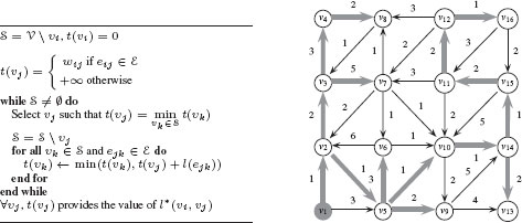
FIGURE 1.7
Left: Dijkstra’s algorithm for computing shortest path from a source vertex υ_i to all vertices in a graph. Right: Illustration of Dijkstra’s algorithm. The source is vertex υ₁. The shortest path from υ₁ to other vertices is shown with bolded grey arrows.

1.4.4    Trees and Minimum Spanning Trees

A tree is an undirected connected graph without cycles (acyclic). An unconnected tree without cycles is called a forest (each connected component of a forest is a tree). More precisely, if $\mathcal{G}$ is a graph with $\left|\mathcal{V}\right|=n$ vertices and if $\mathcal{G}$ is a tree, the following properties are equivalent:

•  $\mathcal{G}$ is connected without cycles,

•  $\mathcal{G}$ is connected and has n − 1 edges,

•  $\mathcal{G}$ has no cycles and has n − 1 edges,

•  $\mathcal{G}$ has no cycles and is maximal for this property (i.e., adding any edge creates a cycle),

•  $\mathcal{G}$ is connected and is minimal for this property (i.e., removing any edge makes the graph disconnected),

•  There exists a unique path between any two vertices of $\mathcal{G}$.

A partial graph ${\mathcal{G}}^{\prime }=\left(\mathcal{V},{ℰ}^{\prime }\right)$ of a connected graph $\mathcal{G}=\left(\mathcal{V},ℰ\right)$ is called a spanning tree of $\mathcal{G}$ if ${\mathcal{G}}^{\prime }$ is a tree. There is at least one spanning tree for any connected graph.

We may define the weight (or cost) of any tree $\mathcal{T}=\left(\mathcal{V},{ℰ}_{\mathcal{T}}\right)$ by

$c\left(\mathcal{T}\right)={\displaystyle \sum _{e_k\in {ℰ}_{\mathcal{T}}}w\left(e_k\right)}.$

(1.11)

A spanning tree of the graph that minimizes the cost (compared to all spanning trees of the graph) is called a minimal spanning tree. The minimal spanning tree of a graph may not be unique. The problem of finding a minimal spanning tree of a graph appears in many applications (e.g., in phone network design). There are several algorithms for finding minimum spanning trees, and we present the one proposed by Prim. The principle of Prim’s algorithm is to progressively build a tree. The algorithm starts from the edge of minimum weight and adds iteratively to the tree the edge of minimum weight among all the possible edges that maintain a partial graph that is acyclic. More precisely, for a graph $\mathcal{G}=\left(\mathcal{V},ℰ\right)$, one progressively constructs from a vertex υ₁ a subset ${\mathcal{V}}^{\prime }$ with $\left\{{\upsilon }_1\right\}\subseteq {\mathcal{V}}^{\prime }\subseteq \mathcal{V}$ and a subset ${ℰ}^{\prime }\subseteq ℰ$ such that the partial graph ${\mathcal{G}}^{\prime }=\left(\mathcal{V},{ℰ}^{\prime }\right)$ is a minimum spanning tree of $\mathcal{G}$. To do this, at each step, one selects the edge e_ij of minimum weight in the set $\left\{e_{kl}|e_{kl}\in ℰ,{\upsilon }_k\in {\mathcal{V}}^{\prime },l\in \mathcal{V}{\mathcal{V}}^{\prime }\right\}$. Subset ${\mathcal{V}}^{\prime }$ and ${ℰ}^{\prime }$ are then augmented with vertex υ_j and edge $e_{ij}:{\mathcal{V}}^{\prime }\leftarrow {\mathcal{V}}^{\prime }\cup \left\{{\upsilon }_j\right\}$ and ${ℰ}^{\prime }\leftarrow {ℰ}^{\prime }\cup \left\{e_{ij}\right\}$. The algorithm terminates when ${\mathcal{V}}^{\prime }=\mathcal{V}$. Prim’s algorithm for computing minimum spanning trees is provided in Figure 1.8 along with an example on a given graph. In computer vision, minimum spanning trees have been used, for example, for image segmentation [16] and image hierarchical representation [17].

1.4.5    Maximum Flows and Minimum Cuts

A transport network is a weighted directed graph $\mathcal{G}=\left(\mathcal{V},ℰ\right)$ such that

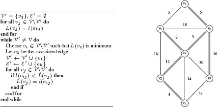
FIGURE 1.8
Left: Prim’s algorithm for computing minimum spanning trees in a graph starting from node υ₁. Note that, any node may be selected as υ₁, and the algorithm will generate a minimal spanning tree. However, when a graph contains multiple minimal spanning trees the selection of υ₁ may determine which minimal spanning tree is determined by the algorithm. Right: Illustration of Prim’s algorithm. The minimum spanning tree is shown by the grey bolded edges.

•  There exists exactly one vertex υ₁ with no predecessor called the source (and denoted by υ_s), that is, deg⁺ (υ₁) = 0,

•  There exists exactly one vertex υ_n with no successor called the sink (and denoted by υ_t), that is, deg⁻ (υ_n) = 0,

•  There exists at least one path from υ_s to υ_t,

•  The weight w(e_ij) of the directed edge e_ij is called the capacity and it is a nonnegative real number, that is, we have a mapping $w:ℰ\to {ℝ}^{+}$.

We denote by ${\mathcal{A}}^{+}\left({\upsilon }_i\right)$ the set of inward directed edges from vertex υ_i:

${\mathcal{A}}^{+}\left({\upsilon }_i\right)=\left\{e_{ji}\in ℰ\right\}.$

(1.12)

Similarly, we denote by ${\mathcal{A}}^{-}\left({\upsilon }_i\right)$ the set of outward directed edges from vertex υ_i:

${\mathcal{A}}^{-}\left({\upsilon }_i\right)=\left\{e_{ij}\in ℰ\right\}.$

(1.13)

A function $\phi :ℰ\to {ℝ}^{+}$ is called a flow iff

•  Each vertex υ_i ∉ {υ_s, υ_t} satisfies the conservation condition (also called Kirchhoff’s Current Law):

${\displaystyle \sum _{e_{ji}}\phi \left(e_{ji}\right)-{\displaystyle \sum _{e_{ij}}\phi \left(e_{ij}\right)}=0,}$

(1.14)

which may also be written in matrix form as

$A^T\mathit{\phi }=p,$

(1.15)

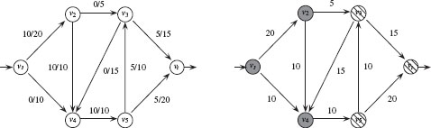
FIGURE 1.9
Left: an (s, t)-flow with value 10. Each edge is labeled with its flow/capacity. Right: An (s, t)-cut with capacity 30, ${\mathcal{V}}_1=\left\{{\upsilon }_s,{\upsilon }_2,{\upsilon }_4\right\}$ (grey) and ${\mathcal{V}}_2=\left\{{\upsilon }_3,{\upsilon }_5,{\upsilon }_t\right\}$ (striped).

where p_i = 0 for any υ_i ∉ {υ_s, υ_t}. Intuitively, this law states that the flow entering each node must also leave that node (i.e., conservation of flow).

•  For each edge e_ij, the capacity constraint φ(e_ij) ≤ w(e_ij) is satisfied.

The value of a flow is $\left|\phi \right|={\displaystyle \sum _{e_{ij}\in \mathcal{A}-\left({\upsilon }_s\right)}\phi \left(e_{ij}\right)}={\displaystyle \sum _{e_{ij}\in \mathcal{A}+\left({\upsilon }_t\right)}\phi \left(e_{ij}\right)}=p_s$. A flow φ* is a maximum flow if its value is the largest possible, that is, |φ*| ≥ |φ| for every other flow φ. Figure 1.9 shows an (s, t) flow with value 10.

An (s, t)-cut is a partition $P=<{\mathcal{V}}_1,{\mathcal{V}}_2>$ of the vertices into subsets ${\mathcal{V}}_1$ and ${\mathcal{V}}_2$, such that, ${\mathcal{V}}_1\cap {\mathcal{V}}_2=\cancel{0},{\mathcal{V}}_1\cup {\mathcal{V}}_2=\mathcal{V},{\upsilon }_s\in {\mathcal{V}}_1$ and ${\upsilon }_t\in {\mathcal{V}}_2$. The capacity of a cut P is the sum of the capacities of the edges that start in ${\mathcal{V}}_1$ and end in ${\mathcal{V}}_2$:

$C\left(P\right)={\displaystyle \sum _{{\upsilon }_i\in {\mathcal{V}}_1}{\displaystyle \sum _{{\upsilon }_j\in {\mathcal{V}}_2}w\left(e_{ij}\right)}},$

(1.16)

with w(e_ij) = 0 if $e_{ij}\notin ℰ$. Figure 1.9 shows an (s, t)-cut with capacity 30. The minimum cut problem is to compute an (s, t)-cut for which the capacity is as low as possible. Intuitively, the minimum cut is the least expensive way to disrupt all flow from υ_s to υ_t. In fact, one can prove that, for any weighted directed graph, there is always a flow φ and a cut $\left({\mathcal{V}}_1,{\mathcal{V}}_2\right)$ such that the value of the maximum flow is equal to the capacity of the minimum cut [18].

We call an edge e_ij saturated by a flow if φ(e_ij) = w_ij. A path from υ_s to υ_t is saturated if any one of its edges is saturated. The residual capacity of an edge $c_r:\mathcal{V}\times \mathcal{V}\to {ℝ}^{+}$ is

$c_r\left(e_{ij}\right)=\{\begin{array}{r}\hfill w_{ij}-\phi \left(e_{ij}\right)\text{if}{e}_{ij}\in ℰ,\\ \hfill \phi \left(e_{ij}\right)\text{if}{e}_{ji}\in ℰ,\\ \hfill 0\text{otherwise}.\end{array}$

(1.17)

The residual capacity represents the flow quantity that can still go through the edge. We may define the residual graph as a partial graph ${\mathcal{G}}_r=\left(\mathcal{V},{ℰ}_r\right)$ of the initial graph where all the edges of zero residual capacity have been removed, that is, ${ℰ}_r=\left\{e_{ij}\in ℰ|c_r\left(e_{ij}\right)>0\right\}$.

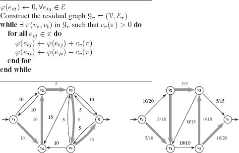
FIGURE 1.10
Top: Ford–Fulkerson algorithm for maximum flow. Bottom: An augmenting path π in ${\mathcal{G}}_r$ with c_r(π) = 5, and the associated augmented flow φ′.

Given a path π in ${\mathcal{G}}_r$ from υ_s to υ_t, the residual capacity of an augmenting path is the minimum of all the residual capacities of its edges:

$c_r\left(\pi \right)=\underset{e_{ij}\in \pi }{\arg \min }{c}_r\left(e_j\right).$

(1.18)

Such a path is called an augmenting path if c_r(π) > 0. From this augmenting path we can define a new augmented flow function φ′:

${\phi }^{\prime }\left(e_{ij}\right)=\{\begin{array}{r}\hfill \phi \left(e_{ij}\right)+c_r\left(\pi \right)\text{if}{e}_{ij}\in \pi ,\\ \hfill \phi \left(e_{ij}\right)-c_r\left(\pi \right)\text{if}{e}_{ji}\in \pi ,\\ \hfill \phi \left(e_{ij}\right)\text{otherwise}.\end{array}$

(1.19)

A flow is called a maximum flow if and only if the corresponding residual graph is disconnected (i.e., there is no augmenting path). There are several algorithms for finding maximum flows, but we present the classic algorithm proposed by Ford and Fulkerson [18]. The principle of the Ford–Fulkerson algorithm is to add flow along one path as long as there exists an augmenting path in the graph. Figure 1.10 provides the algorithm along with one step of generating an augmenting path. In computer vision, the use of maximum-flow/min-cut solutions to solve problems is typically referred to as graph cuts, following the publication by Boykov et al. [19]. Furthermore, the Ford–Fulkerson algorithm was found to be inefficient for many computer vision problems, with the algorithm by Boykov and Kolmogorov generally preferred [20].

1.5    Graph Models in Image Processing and Analysis

In the previous sections we have presented some of the basic definitions and notations used for graph theory in this book. These definitions and notations may be found in other sources in the literature but were presented to make this work self-contained. However, there are many ways in which graph theory is applied in image processing and computer vision that are specialized to these domains. We now build on the previous definitions to provide some of the basics for how graph theory has been specialized for image processing and computer vision in order to provide a foundation for the subsequent chapters.

1.5.1    The Regular Lattice

Digital image processing operates on sampled data from an underlying continuous light field. Each sample is called a pixel in 2D or a voxel in 3D. The sampling is based on the notion of lattice, which can be viewed as a regular tiling of a space by a primitive cell. A d-dimensional lattice ${\mathbb{L}}^d$ is a subset of the d-dimensional Euclidean space ${ℝ}^d$ with

${\mathbb{L}}^d=\left\{x\in {ℝ}^d|x={\displaystyle \sum _{i=1}^d{k}_i{u}_i,k_i\in \mathbb{Z}}\right\}=U{\mathbb{Z}}^d,$

(1.20)

where $u_1,\dots ,u_d\in {ℝ}^d$ form a basis of ${ℝ}^d$ and U is the matrix of column vectors. A lattice in a d-dimensional space is therefore a set of all possible vectors represented as integer weighted combinations of d linearly independent basis vectors. The lattice points are given by Uk with $k^T=\left(k_1,\dots ,k_d\right)\in {\mathbb{Z}}^d$.

The unit cell of ${\mathbb{L}}^d$ with respect to the basis u₁, …, u_d is

$C=\left\{x\in {ℝ}^d|x={\displaystyle \sum _{i=1}^d{k}_i{u}_i,k_i\in \left[0,1\right]}\right\}=U\cdot {\left[0,u_1\right]}^d,$

(1.21)

where [0, u₁]^d is the unit cube in ${ℝ}^d$. The volume of C is given by |det U|. The density of the lattice is given by 1/|detU|, that is, the lattice sites per unit surface. The set $\left\{C+x|x\in {ℝ}^d\right\}$ of all lattice cells covers ${ℝ}^d$. The Voronoi cell of a lattice is called the unit cell (a cell of a lattice whose translations cover the whole space). The Voronoi cell encloses all points that are closer to the origin than to other lattice points. The Voronoi cell boundaries are equidistant hyperplanes between surrounding lattice points. Two well-known 2D lattices are the rectangular $U_1=\left[\begin{array}{cc}1& 0\\ 0& 1\end{array}\right]$ and hexagonal $U_2=\left[\begin{array}{cc}\frac{\sqrt{3}}{2}& 0\\ \frac{1}{2}& 1\end{array}\right]$ lattices. Figure 1.11 presents these two lattices. By far the most common lattice in image processing and computer vision is the rectangular sampling lattice derived from U₁. In 3D image processing, the lattice sampling is typically given by

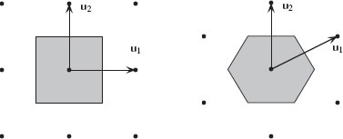
FIGURE 1.11
The rectangular (left) and hexagonal (right) lattices and their associated Voronoi cells.

$U_3=\left[\begin{array}{ccc}1& 0& 0\\ 0& 1& 0\\ 0& 0& k\end{array}\right],$

(1.22)

for some constant k in which the typical situation is that k ≥ 1.

The most common way of using a graph to model image data is to identify every node with a pixel (or voxel) and to impose an edge structure to define local neighborhoods for each node. Since a lattice defines a regular arrangement of pixels it is possible to define a regular graph by using edges to connect pairs of nodes that fall within a fixed Euclidean distance of each other.

For example, in a rectangular lattice, two pixels p = (p₁, p₂)^T and q = (q₁, q₂)^T of ${\mathbb{Z}}^2$, are called 4-adjacent (or 4-connected) if they differ by at most one coordinate:

$\left|p_1-q_1\right|+\left|p_2-q_2\right|=1,$

(1.23)

and 8-adjacent (or 8-connected) if they differ at most of 2 coordinates:

$\max \left(\left|p_1-q_1\right|,\left|p_2-q_2\right|\right)=1,$

(1.24)

In the hexagonal lattice, only one adjacency relationship exists: 6-adjacency. Figure 1.11 presents adjacency relationships on the 2D rectangular and hexagonal lattices. Similarly, in ${\mathbb{Z}}^3$, we can say in a rectangular lattice that voxels are 6-adjacent, 18-adjacent, or 26-adjacent whether they differ at most of 1, 2, or 3 coordinates. Figure 1.12 presents adjacency relationships between 3D cells (voxels).

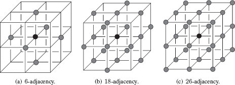
FIGURE 1.12
Different adjacency structures in a 3D lattice.

If one considers edges that connect pairs of nodes that are not directly (i.e., locally) spatially adjacent (e.g., 4- or 8-connected in ${\mathbb{Z}}^2$) [21], the corresponding edges are called nonlocal edges [22]. The level of nonlocality of an edge depends on how far the two points are in the underlying domain. These nonlocal edges are usually obtained from proximity graphs (see Section 1.5.3) on the pixel coordinates (e.g., ϵ-ball graphs) or on pixel features (e.g., k-nearest-neighbor graphs on patches).

1.5.2    Irregular tessellations

Image data is almost always sampled in a regular, rectangular lattice that is modeled with the graphs in the previous section. However, images are often simplified prior to processing by merging together regions of adjacent pixels using an untargeted image segmentation algorithm. The purpose of this simplification is typically to reduce processing time for further operations, but it can also be used to compress the image representation or to improve the effectiveness of subsequent operations. When this image simplification has been performed, a graph may be associated with the simplified image by identifying each merged region with one node and defining an edge relationship for two adjacency regions. Unfortunately, this graph is no longer guaranteed to be regular due to the image-dependent and space-varying merging of the underlying pixels. In this section we review common simplification methods that produce these irregular graphs.

One very well-known irregular image tessellation is the region quadtree tessellation [25]. A region quadtree is a hierarchical image representation that is derived from recursively subdividing the 2D space into four quadrants of equal size until every square contains one homogeneous region (based on appearance properties of every region of the underlying rectangular grid) or contains a maximum of one pixel. A region quadtree tesselation can be easily represented by a tree where each node of the tree corresponds to a square. The set of all nodes at a given depth provides a given level of decomposition of the 2D space. Figure 1.13 presents a simple example on an image (Figure 1.13(a)) with the associated tree (Figure 1.13(b)), as well as an example on a real image (Figure 1.13(c)). Quadtrees easily generalize to higher dimensions. For instance, in three dimensions, the 3D space is recursively subdivided into eight octants, and thus the tree is called an octree, where each node has eight children.

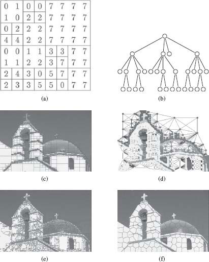
FIGURE 1.13
(a) An image with the quadtree tessellation, (b) the associated partition tree, (c) a real image with the quadtree tessellation, (d) the region adjacency graph associated to the quadtree partition, (e) and (f) two different irregular tessellations of an image using image-dependent superpixel segmentation methods: Watershed [23] and SLIC superpixels [24].

Finally, any partition of the classical rectangular grid can be viewed as producing an irregular tessellation of an image. Therefore any segmentation of an image can be associated with a region adjacency graph. Figure 1.13(d) presents the region adjacency graph associated to the partition depicted in 1.13(c). Specifically, given a graph $\mathcal{G}=\left\{\mathcal{V},ℰ\right\}$ where each node is identified with a pixel, a partition into R connected regions ${\mathcal{V}}_1\cup {\mathcal{V}}_2\cup \dots \cup {\mathcal{V}}_R=\mathcal{V},{\mathcal{V}}_1\cap {\mathcal{V}}_2\cap \dots \cap {\mathcal{V}}_R=\cancel{0}$ may be identified with a new graph $\tilde{\mathcal{G}}=\left\{\tilde{\mathcal{V}},\widetilde{ℰ}\right\}$ where each partition of $\mathcal{V}$ is identified with a node of $\tilde{\mathcal{V}}$, that is, ${\mathcal{V}}_i\in \tilde{\mathcal{V}}$. A common method for defining $\widetilde{ℰ}$ is to let the edge weight between each new node equal the sum of the edge weights connecting each original node in the sets, that is, for edge $e_{ij}\in \widetilde{ℰ}$

$w_{ij}={\displaystyle \sum _{e_{ks},{\upsilon }_k\in {\mathcal{V}}_i,{\upsilon }_s\in {\mathcal{V}}_j}{w}_{ks}}.$

(1.25)

Each contiguous ${\mathcal{V}}_i$ is called a superpixel. Superpixels are an increasingly popular trend in computer vision and image processing. This popularity is partly due to the success of graph-based algorithms, which can be used to operate efficiently on these irregular structures (as opposed to traditional image-processing algorithms which required that each element is organized on a grid). Indeed, graph-based models (e.g., Markov Random Fields or Conditional Random Fields) can provide dramatic speed increases when moving from pixel-based graphs to superpixel-based graphs due to the drastic reduction in the number of nodes. For many vision tasks, compact and highly uniform superpixels that respect image boundaries are desirable. Typical algorithms for generating superpixels are Normalized Cuts [21], Watersheds [23], Turbo Pixels [26], and simple linear iterative clustering superpixels [24], etc. Figure 1.13(e) and (f) presents some irregular tessellations based on superpixel algorithms.

1.5.3    Proximity Graphs for Unorganized Embedded Data

Sometimes the relevant features of an image are neither individual pixels nor a partition of the image. For example, the relevant features of an image might be the blood cells in a biomedical image, and it is these blood cells that we wish to identify with the nodes of our graph. We may assume that each node (feature) in a dD image is associated with a coordinate in d dimensions. However, although each node has a geometric representation, it is much less clear than before how to construct a meaningful edge set for a graph based on the proximity of features.

There are many ways to construct a proximity graph representation from a set of data points that are embedded in ${ℝ}^d$. Let us consider a set of data points $\left\{x_1,\dots ,x_n\right\}\in {ℝ}^d$. To each data point we associate a vertex of a proximity graph $\mathcal{G}$ to define a set of vertices $\mathcal{V}=\left\{{\upsilon }_1,{\upsilon }_2,\dots ,{\upsilon }_n\right\}$. Determining the edge set $ℰ$ of the proximity graph $\mathcal{G}$ requires defining the neighbors of each vertex υ_i according to its embedding x_i. A proximity graph is therefore a graph in which two vertices are connected by an edge iff the data points associated to the vertices satisfy particular geometric requirements. Such particular geometric requirements are usually based on a metric measuring the distance between two data points. A usual choice of metric is the Euclidean metric. We will denote as $\mathcal{D}\left({\upsilon }_i,{\upsilon }_j\right)={\Vert x_i-x_j\Vert }_2$ the Euclidean distance between vertices, and as $\mathcal{B}\left({\upsilon }_i;r\right)=\left\{x_j\in {ℝ}^n|\mathcal{D}\left({\upsilon }_i,{\upsilon }_j\right)\le r\right\}$ the closed ball of radius r centered on x_i. Classical proximity graphs are:

•  The ϵ-ball graph: υ_i ~ υ_j if $x_j\in \mathcal{B}\left({\upsilon }_i;ϵ\right)$.

•  The k-nearest-neighbor graph (k-NNG): υ_i ~ υ_j if the distance between x_i and x_i is among the k-th smallest distances from x_i to other data points. The k-NNG is a directed graph since one can have x_i among the k-nearest neighbors of x_j but not vice versa.

•  The Euclidean Minimum Spanning Tree (EMST): This is a connected tree subgraph that contains all the vertices and has a minimum sum of edge weights (see Section 1.4.4). The weight of the edge between two vertices is the Euclidean distance between the corresponding data points.

•  The symmetric k-nearest-neighbor graph (Sk-NNG): υ_i ~ υ_j if x_i is among the k-nearest neighbors of y or vice versa.

•  The mutual k-nearest-neighbor graph (Mk-NNG): υ_i ~ υ_j if x_i is among the k-nearest neighbors of y and vice versa. All vertices in a mutual k-NN graph have a degree upper-bounded by k, which is not usually the case with standard k-NN graphs.

•  The Relative Neighborhood Graph (RNG): υ_i ~ υ_j iff there is no vertex in

$\mathcal{B}\left({\upsilon }_i;\mathcal{D}\left({\upsilon }_i,{\upsilon }_j\right)\right)\cap \mathcal{B}\left({\upsilon }_j;\mathcal{D}\left({\upsilon }_i,{\upsilon }_j\right)\right).$

(1.26)

•  The Gabriel Graph (GG): υ_i ~ υ_j iff there is no vertex in

$\mathcal{B}\left(\frac{{\upsilon }_i+{\upsilon }_j}{2};\frac{\mathcal{D}\left({\upsilon }_i,{\upsilon }_j\right)}{2}\right).$

(1.27)

•  The β-Skeleton Graph (β-SG): υ_i ~ υ_j iff there is no vertex in

$\mathcal{B}\left(\left(1-\frac{\beta }{2}\right){\upsilon }_i+\frac{\beta }{2}{\upsilon }_j;\frac{\beta }{2}\mathcal{D}\left({\upsilon }_i,{\upsilon }_j\right)\right)\cap \mathcal{B}\left(\left(1-\frac{\beta }{2}\right){\upsilon }_j+\frac{\beta }{2}{\upsilon }_i;\frac{\beta }{2}\mathcal{D}\left({\upsilon }_i,{\upsilon }_j\right)\right).$

(1.28)

The Gabriel Graph is obtained with β = 1, and the Relative Neighborhood Graph with β = 2.

•  The Delaunay Triangulation (DT): υ_i ~ υ_j iff there is a closed ball $\mathcal{B}\left(\cdot ;r\right)$ with υ_i and υ_j on its boundary and no other vertex υ_k contained in it. The Delaunay Triangulation is the dual of the Voronoi irregular tessellation where each Voronoi cell is defined by the set {$x\in {ℝ}^n|\mathcal{D}\left(x,{\upsilon }_k\right)\le \mathcal{D}\left(x,{\upsilon }_j\right)$ for all υ_j ≠ υ_k}. In such a graph, ∀ υ_i, deg (υ_i) = 3.

•  The Complete Graph (CG): υ_i ~ υ_j ∀(υ_i, υ_j), that is, it is a fully connected graph that contains an edge for each pair of vertices and $ℰ=\mathcal{V}\times \mathcal{V}$.

A surprising relationship between the edge sets of these graphs is that [27]

$1-\text{NNG}\subseteq \text{EMST}\subseteq \text{RNG}\subseteq \text{GG}\subseteq \text{DT}\subseteq \text{CG}\text{.}$

(1.29)

Figure 1.14 presents examples of some of these proximity graphs. All these graphs are extensively used in different image analysis tasks. These methods have been used in Scientific Computing to obtain triangular irregular grids (triangular meshes) adapted for the finite element method [28] for applications in physical modeling used in industries such as automotive, aeronautical, etc. Proximity graphs have also been used in Computational and Discrete Geometry [29] for the analysis of point sets in ${ℝ}^2$ (e.g., for 2D shapes) or ${ℝ}^3$ (e.g., for 3D meshes). They are also the basis of many classification and model reduction methods [30] that operate on feature vectors in ${ℝ}^d$, for example, Spectral Clustering [31], Manifold Learning [32], object matching, etc. Figure 1.15 presents some proximity graph examples on real-world data.

1.6    Conclusion

Graphs are tools that make it possible to model pairwise relationships between data elements and have found wide application in science and engineering. Computer vision and image processing have a long history of using graph models, but these models have been increasingly dominant representations in the recent literature. Graphs may be used to model spatial relationships between nearby or distant pixels, between image regions, between features, or as models of objects and parts. The subsequent chapters of this book are written by leading researchers who will provide the reader with a detailed understanding of how graph theory is being successfully applied to solve a wide range of problems in computer vision and image processing.

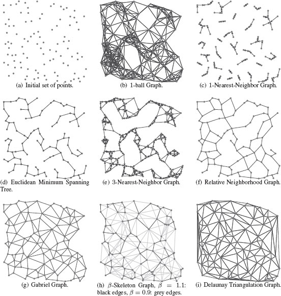
FIGURE 1.14
Examples of proximity graphs from a set of 100 points in ${\mathbb{Z}}^2$.

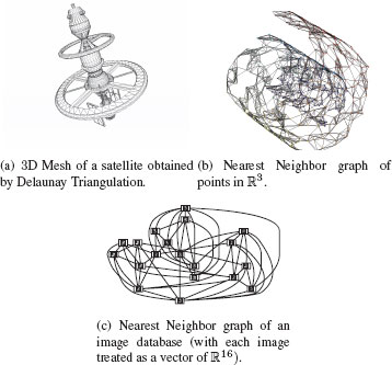
FIGURE 1.15
Some proximity graph examples on real-world data.

Bibliography

[1]  N. Biggs, E. Lloyd, and R. Wilson, Graph Theory, 1736–1936. Oxford University Press, New-York, 1986.

[2]  A.-L. Barabasi, Linked: How Everything Is Connected to Everything Else and What It Means. Plume, New-York, 2003.

[3]  D. J. Watts, Six Degrees: The Science of a Connected Age. W. W. Norton, 2004.

[4]  N. A. Christakis and J. H. Fowler, Connected: The Surprising Power of Our Social Networks and How They Shape Our Lives. Little, Brown and Company, 2009.

[5]  F. Harary, Graph Theory. Addison-Wesley, 1994.

[6]  A. Gibbons, Algorithmic Graph Theory. Cambridge University Press, 1989.

[7]  N. Biggs, Algebraic Graph Theory, 2nd ed. Cambridge University Press, 1994.

[8]  R. Diestel, Graph Theory, 4th ed., ser. Graduate Texts in Mathematics. Springer-Verlag, 2010, vol. 173.

[9]  J. L. Gross and J. Yellen, Handbook of Graph Theory, ser. Discrete Mathematics and Its Applications. CRC Press, 2003, vol. 25.

[10]  J. Bondy and U. Murty, Graph Theory, 3rd ed., ser. Graduate Texts in Mathematics. Springer-Verlag, 2008, vol. 244.

[11]  J. Gallier, Discrete Mathematics, 1st ed., ser. Universitext. Springer-Verlag, 2011.

[12]  L. Grady and J. R. Polimeni, Discrete Calculus: Applied Analysis on Graphs for Computational Science. Springer, 2010.

[13]  E. W. Dijkstra, “A note on two problems in connexion with graphs,” Numerische Mathematik, vol. 1, no. 1, pp. 269–271, 1959.

[14]  E. N. Mortensen and W. A. Barrett, “Intelligent scissors for image composition,” in SIGGRAPH, 1995, pp. 191–198.

[15]  P. Felzenszwalb and R. Zabih, “Dynamic programming and graph algorithms in computer vision,” IEEE Trans. Pattern Anal. Mach. Intell., vol. 33, no. 4, pp. 721–740, 2011.

[16]  P. F. Felzenszwalb and D. P. Huttenlocher, “Efficient graph-based image segmentation,” Int. J. Computer Vision, vol. 59, no. 2, pp. 167–181, 2004.

[17]  L. Najman, “On the equivalence between hierarchical segmentations and ultrametric watersheds,” J. of Math. Imaging Vision, vol. 40, no. 3, pp. 231–247, 2011.

[18]  L. Ford Jr and D. Fulkerson, “A suggested computation for maximal multi-commodity network flows,” Manage. Sci., pp. 97–101, 1958.

[19]  Y. Boykov, O. Veksler, and R. Zabih, “Fast approximate energy minimization via graph cuts,” IEEE Trans. Pattern Anal. Mach. Intell., vol. 23, no. 11, pp. 1222–1239, 2001.

[20]  Y. Boykov and V. Kolmogorov, “An experimental comparison of min-cut/max-flow algorithms for energy minimization in vision,” IEEE Trans. Pattern Anal. Mach. Intell., vol. 26, no. 9, pp. 1124–1137, 2004.

[21]  J. Shi and J. Malik, “Normalized cuts and image segmentation,” IEEE Trans. Pattern Anal. Mach. Intell., vol. 22, no. 8, pp. 888–905, 2000.

[22]  A. Elmoataz, O. Lezoray, and S. Bougleux, “Nonlocal discrete regularization on weighted graphs: A framework for image and manifold processing,” IEEE Trans. Image Process., vol. 17, no. 7, pp. 1047–1060, 2008.

[23]  L. Vincent and P. Soille, “Watersheds in digital spaces: An efficient algorithm based on immersion simulations,” IEEE Trans. Pattern Anal. Mach. Intell., vol. 13, no. 6, pp. 583–598, 1991.

[24]  A. Radhakrishna, “Finding Objects of Interest in Images using Saliency and Superpixels,” Ph.D. dissertation, 2011.

[25]  H. Samet, “The quadtree and related hierarchical data structures,” ACM Comput. Surv., vol. 16, no. 2, pp. 187–260, 1984.

[26]  A. Levinshtein, A. Stere, K. N. Kutulakos, D. J. Fleet, S. J. Dickinson, and K. Siddiqi, “Turbopixels: Fast superpixels using geometric flows,” IEEE Trans. Pattern Anal. Mach. Intell., vol. 31, no. 12, pp. 2290–2297, 2009.

[27]  G. T. Toussaint, “The relative neighbourhood graph of a finite planar set,” Pattern Recogn., vol. 12, no. 4, pp. 261–268, 1980.

[28]  O. Zienkiewicz, R. Taylor, and J. Zhu, The Finite Element Method: Its Basis and Fundamentals, 6th ed. Elsevier, 2005.

[29]  J. E. Goodman and J. O’Rourke, Handbook of Discrete and Computational Geometry, 2nd ed. CRC Press LLC, 2004.

[30]  M. A. Carreira-Perpinan and R. S. Zemel, “Proximity graphs for clustering and manifold learning,” in NIPS, 2004.

[31]  U. von Luxburg, “A tutorial on spectral clustering,” Stat. Comp., vol. 17, no. 4, pp. 395–416, 2007.

[32]  J. A. Lee and M. Verleysen, Nonlinear Dimensionality Reduction. Springer, 2007.

¹Edge weights may be used to represent either affinities or distances between nodes. An affinity weight of zero is viewed as equivalent to a disconnection (removal of the edge from $ℰ$), and a distance weight of ∞ is viewed as equivalent to a disconnection. An affinity weight a may be converted to a distance weight b via $b=\frac{1}{a}$. A much longer discussion on this relationship may be found in [12]. In this work, affinity weights and distance weights use the same notation, with the distinction being made by context. All weights in this section are considered to be distance weights.