10 Optimal Simultaneous Multisurface and Multiobject Image Segmentation

Images are increasingly occurring as higher-dimensional data. While the early effort was devoted to developing methods for image processing and analysis in 2D, the focus has later shifted to stereo images, 2D + time (motion video) image data, and to multispectral (or multiband) 3D images. Substantial effort has been devoted to developing automated or semi-automated image segmentation techniques over the past decades [1]. With the increased availability of X-ray computed tomography (CT), magnetic resonance (MR), positron-emission tomography (PET), singlephoton emission computed tomography (SPECT), ultrasound, optical coherence tomography (OCT), and other medical imaging modalities, higher-dimensional data are omnipresent in routine clinical medicine. Clearly, 3D, 4D, and 5D volumetric images are becoming common. In this context, 3D images represent volumetric data typically organized as a x–y–z matrices. When adding temporal image acquisition aspects, the image data become four-dimensional (x–y–z–t matrices) – MR, CT, or ultrasound images of cardiac ventricles obtained over cardiac cycle may serve as an example of such 4D datasets. When such 4D image data are acquired at several time instances over time, for example, weekly over a period of several weeks, 5D image data result (x–y–z–t₁–t₂ matrices) — pulmonary CT images acquired over one breathing cycle and longitudinally over several imaging sessions are an example of such 5D image data. It is easily possible to imagine how higher-dimensional image data can be formed. Same as conventional 2D image data, high-dimensional image data need to be processed, segmented, analyzed, and used for intelligent decision making. However, the n-D character of the underlying image data requires development of fundamentally different approaches, in which contextual information across all dimensions of such images is considered and inherently incorporated. In no other image analysis step is this more apparent than in image segmentation.

Incorporating image-based contextual information and performing image segmentation in an optimal fashion are two powerful concepts that form the basis of the n-dimensional graph-based image segmentation approaches described below [2, 3, 4]. After introducing the basic algorithm on a simple 2D example, a general methodology for optimal segmentation of single surfaces is introduced that is applicable to n-D image data. Extensions facilitating optimal segmentation of multiple interacting surfaces for a single or multiple interacting objects are reported. The generality of the approach is demonstrated on closed-surface and multiobject segmentation cases and applicability to n-D image data is shown. Since the optimality of the solution is guaranteed with respect to the cost function, special emphasis is given to cost function design, including edge-based, region-based, and edge-region-combined cost functions. Methods for incorporating shape priors are discussed leading to arc-based graph representation and associated arc-based graph segmentation solutions.

10.2 Motivation and Problem Description

As mentioned, n-dimensional images are routinely occurring in medical imaging applications worldwide. With the ever-increasing numbers of such acquired image data, with ever-increasing numbers of image slices forming such images, and with increased in-plane image resolution, the image data amounts that require expert analysis by radiologists, orthopedists, internists, and other medical professionals are growing rapidly and exceed the capability of physicians to analyze them visually. Performing organ/object segmentations in 3D, 4D, or higher-D is infeasible for a human observer in a clinical setting due to the time constraints and the overall tedious character of manual tracing. The functionality and performance of the reported automated methods is demonstrated in a variety of medical image analysis tasks providing a convincing evidence of the broad applicability of the introduced algorithmic concepts.

The segmentation problems we are addressing in this chapter can be divided in the following categories, all of them applicable to n-D image data:

• Single-surface terrain-like segmentation, for example diaphragm segmentation in 3D or 4D CT images.

• Multisurface terrain-like segmentation, e.g., segmentation of multiple retinal layers from 3D OCT images.

• Single-/multisurface segmentation of tubular objects, like detection of vascular inner and outer wall in 3D/4D intravascular ultrasound.

• Single-/multisurface segmentation of closed surfaces, e.g., identification of a liver surface from 3D CT or detection of endo- and epi-cardial surfaces of cardiac left ventricle from 3D/4D/5D ultrasound.

• Single-/multisurface segmentation of bifurcating tubular structures, e.g., inner and outer walls of intrathoracic airway trees across bifurcations from 3D CT images.

• Single-/multisurface segmentation of several mutually interacting objects, like simultaneous detection of prostate and bladder from CT or simultaneous segmentation of knee bones and cartilages from MR images.

In all of these and many similar cases, the underlying image data are used to construct a graph in which optimal surfaces are identified according to a node- or arc-based cost function. Importantly, all cases for which the reported approach is applicable require that the graph columns intercept the sought surface (or surfaces) exactly once. Having this constraint is advantageous in applications for which it is imperative to preserve object topology, which is different from the label-based approaches of [5, 6]. To satisfy this requirement, the graph must be formed correspondingly, either by using a priori information about the approximate shape and/or topology of the resulting object(s), or by performing topologically correct approximate presegmentation that is used for graph construction. Details of these processes are given below.

10.3 Methods for Graph-Based Image Segmentation

10.3.1 Optimal Surface Detection Problems

Let $ℐ$ be a given 3-D volumetric image with size of n = X × Y × Z. Figure 10.1(a) shows a 3-D retinal OCT volume. For each (x, y) pair, 0 ≤ x < X and 0 ≤ y < Y, the voxel subset ${ℐ (x, y, z) | 0 \leq z < Z}$ forms a column parallel to the z-axis, denoted by Col(x, y). Two columns are adjacent if their (x, y) coordinates satisfy some neighborhood conditions. For instance, under the 4-neighbor setting, the column Col(x, y) is adjacent to Col(x′, y′) if $| x - x^{'} | + | y - y^{'} | = 1$ . Henceforth, we use a model of the 4-neighbor adjacency; this simple model can be easily extended to other adjacency settings. Note that each of the sought z-monotone surfaces contains exactly one voxel in each column of $ℐ$ . Denote by S(x, y) the z-coordinate of the voxel $ℐ (x, y, z)$ on a surface S. Figure 10.1(b) shows the surface orientation. The surface smoothness constraint is specified by two smoothness parameters, Δx and Δy, which define the maximum allowed change in the z-coordinate of a surface along each unit distance change in the x and y dimensions, respectively. If $ℐ (x, y, z^{'})$ and $ℐ (x + 1, y, z^{″})$ (respectively, $ℐ (x, y + 1, z^{″})$ ) are two (neighboring) voxels on a feasible surface, then |z′−z″| ≤ Δx (respectively, |z′−z″| ≤ Δy) (Figure 10.1(c)). More precisely, a surface in I is defined as a function S : [0..X) × [0..Y) → [0..Z), such that for any pair (x, y), |S(x, y) − S(x + 1, y)| ≤ Δx and |S(x, y) − S(x, y + 1)| ≤ Δy, where [a..b) denotes the set of integers from a to b − 1. In multiple surface detection, for each pair of the sought surfaces S and S′, we use two parameters, δ^l ≥ 0 and δ^u ≥ 0, to represent the surface separation constraint, which defines the relative positioning and the distance range of the two surfaces. That is, if $ℐ (x, y, z) \in S$ and $ℐ (x, y, z^{'}) \in S^{'}$ , we have δ^l ≤ z′ − z ≤ δ^u for every (x, y) pair (Figure 10.2). A set of surfaces are considered feasible if each individual surface in the set satisfies the given smoothness constraints and if each pair of surfaces satisfies the surface separation constraints.

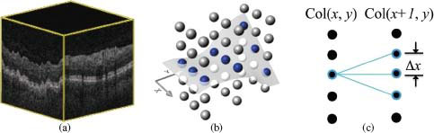
FIGURE 10.1
The optimal surface detection problem. (a) A 3-D retinal OCT volume. (b) The surface orientation. (c) Two adjacent columns with the smoothness parameters Δx = 1.

Designing appropriate cost functions is of paramount importance for any optimization-based segmentation method. The cost function for each voxel in the input image usually reflects either edge-based and/or region-based properties of the target surface, depending on the imaging setting.

Edges defined by image gradients are commonly used for image segmentation. A typical edge-based cost function aims to accurately position the boundary surface in the volumetric image. Incorporating regional information, which alleviates the sensitivity of the initial model and improves the robustness, is becoming increasingly important in image segmentation [7, 8, 9, 10, 11, 12, 13]. We thus assign costs to every voxel of $ℐ$ to integrate the edge- and region-based cost functions, as follows. Each voxel $ℐ (x, y, z)$ has an edge-based cost b_i(x, y, z), which is an arbitrary real value, for the detection of the i-th surface. Note that λ surfaces $S = {S_{1}, S_{2}, \dots, S_{λ}}$ in $ℐ$ induce λ + 1 regions {R₀, R₁, …, R_λ} (Figure 10.2(a)). For each region R_i (i = 0, 1, …, λ), every voxel $ℐ (x, y, z)$ is assigned a real-valued region-based cost c_i (x, y, z). The edge-based cost of each voxel in $ℐ$ is inversely related to the likelihood that it may appear on a desired surface, while the region-based costs c_i(·) (i = 0, 1, …, λ) measure the inverse likelihood of a given voxel preserving the expected regional properties (e.g., homogeneity) of the partition {R₀,R₁, …, R_λ}. Both the edge-based and region-based costs can be determined by using simple low-level image features [1, 8, 9, 12]. Then, the total cost $α (S)$ induced by the λ surfaces in $S$ is defined as

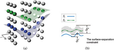
FIGURE 10.2
(a) Two sought surfaces divide the image $ℐ$ into three regions. (b) The surface interrelation modeling with the minimum (δ^l) and maximum (δ^u) surface distances.

$α (S) = \sum_{i = 1}^{λ} b_{i} (S_{i}) + \sum_{i = 0}^{λ} c_{i} (R_{i}) = \sum_{i = 1}^{λ} \sum_{ℐ (x, y, z) \in S_{i}} b_{i} (x, y, z) + \sum_{i = 0}^{λ} \sum_{ℐ (x, y, z) \in R_{i}} c_{i} (x, y, z) .$

(10.1)

10.3.2 Optimal Single Surface Detection

This section presents the polynomial time algorithm for solving the optimal single surface detection (OSSD) problem, in which λ = 1 and no region-based costs are considered, that is, the energy function is $α (S) = \sum_{I (x, y, z) \in S} b (x, y, z)$ . We first exploit the intralayer self-closure structure of the OSSD problem, and then formulate it as a minimum-cost closed set problem based on a nontrivial graph transformation scheme.

A closed set $C$ in a directed graph with arbitrary vertex costs w(·) is a subset of vertices such that all successors of any vertex in $C$ are also contained in $C$ [14, 15].

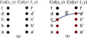
FIGURE 10.3
Illustrating the intralayer self-closure structure of the OSSD problem. The surface smoothness parameter Δx = 1. (a) The lowest neighbors. If voxel c ∈ Col(x, y) is on a feasible surface, then only one of the voxels {b′, c′, d′} on Col(x + 1, y) can be on the same surface. Thus, b′ is the lowest neighbor of voxel c on Col(x + 1, y). The lowest neighbor of voxel a′ ∈ Col(x + 1, y) on Col(x, y) is voxel a. (b) The intralayer self-closure structure. S is a feasible surface. The red voxels form the set Lw(S). The lowest neighbor of each voxel in Lw(S) is also in Lw(S).

The cost of a closed set $C$ , denoted by $w (C)$ , is the total cost of all vertices in $C$ . Note that a closed set can be empty (with a cost zero). The minimum-cost closed set problem seeks a closed set in the graph whose cost is minimized.

10.3.2.1 The Intralayer Self-Closure Property of the OSSD Problem

The algorithm for the OSSD problem hinges on the following observation about the self-closure structure of any feasible OSSD solution. For a voxel $ℐ (x, y, z)$ and each adjacent column Col(x′, y′) of Col(x, y), the lowest neighbor of $ℐ (x, y, z)$ on Col(x′, y′) is the voxel on Col(x′, y′) with the smallest z-coordinate that can appear together with $ℐ (x, y, z)$ on the same feasible surface in $ℐ$ . More precisely, the lowest neighbor of $ℐ (x, y, z)$ on its adjacent column Col(x ± 1, y) (respectively, Col(x, y ± 1)) is $ℐ (x \pm 1, y, \max {0, z - Δ x})$ (respectively, $ℐ (x, y \pm 1, \max {0, z - Δ y})$ ). In Figure 10.3(a), the lowest neighbor of voxel c on Col(x + 1, y) is b′ and the lowest neighbor of voxel a′ on Col(x, y) is voxel a, where Δx = 1.

We say that a voxel $ℐ (x, y, z)$ is below a surface S if S(x, y) > z, and denote by Lw(S) all the voxels of $ℐ$ that are on or below S. A key observation is that for any feasible surface S in $ℐ$ , the lowest neighbors of every voxel in Lw(S) are also contained in Lw(S). Figure 10.3(b) shows the intralayer self-closure structure for two adjacent columns. For instance, the lowest neighbor b′ of voxel c ∈ Lw(S) on Col(x+1, y) is in Lw(S) and the lowest-neighbor c of voxel d′ ∈ Lw(S) on Col(x, y) is also in Lw(S). This intralayer self-closure property is crucial to our algorithm and suggests to relate our target problem to the minimum closed set problem. In our approach, instead of finding an optimal surface S* directly, we seek in $ℐ$ a voxel set Lw(S*), which uniquely defines the surface S *.

10.3.2.2 The Graph Transformation Scheme for the OSSD Problem

This section presents the construction of the node-weighted directed graph $G = (V, ℰ)$ from the input image $ℐ$ , which enables to detect an optimal single surface by computing a minimum-cost closed set. This construction crucially relies on the intralayer self-closure structure.

The directed graph $G$ is constructed, as follows. Every node $υ (x, y, z) \in V$ represents exactly one voxel $ℐ (x, y, z) \in ℐ$ . The graph $G$ can be viewed as a geometric graph defined on a 3-D grid. To abuse the notation, we also use Col(x, y) to denote the nodes in $G$ corresponding to the voxels of Col(x, y) in $ℐ$ . The arcs of $G$ (an arc is a directed edge in a graph) are then introduced to guarantee that all nodes corresponding the voxel set Lw(S) of a feasible surface S form a closed set in $G$ . First, we need to make sure that if voxel $ℐ (x, y, z_{s})$ is on S, then all the nodes υ(x, y, z) of $G$ below υ(x, y, z_s) (with z ≤ z_s) on the same column must be in a closed set $C$ . Thus, for each column Col(x, y), every node υ(x, y, z) (z > 0) has a directed arc to the node υ(x, y, z – 1) immediately below it. These arcs are called the intracolumn arcs, which, in fact, enforce the monotonicity of the sought surface (the sought surface intersects each column exactly once). Next, we need to incorporate into $G$ the smoothness constraints along the x- and y-dimensions. Notice that if voxel $ℐ (x, y, z_{s})$ is on surface S, then its neighboring voxels on S along the x-dimension must be no “lower” than voxel $ℐ (x, y, z_{s} - Δ x)$ . Hence, node $υ (x, y, z_{s}) \in C$ indicates that nodes υ(x + 1, y, z_s − Δx) and υ(x − 1, y, z_s − Δx) must be in $C$ . Thus, for each node υ(x, y, z), we put arcs from υ(x, y, z) to υ(x + 1, y, z – Δx) and to υ(x – 1, y, z – Δ x), respectively. Note that node υ(x + 1, y, z – Δx) (respectively, υ(x − 1, y, z − Δx)) corresponds to the lowest neighbor of voxel $ℐ (x, y, z)$ on its adjacent column Col(x + 1, y) (respectively, Col(x − 1, y)). Those arcs are called the intercolumn arcs. Here, to avoid cluttering the exposition of our key ideas, we do not consider the boundary conditions, which can be handled as well. The same construction is done for the y-dimension.

To incorporate the edge-based costs, a node cost w(x, y, z) is assigned to each node υ(x, y, z) in $G$ , as follows.

$w (x, y, z) = {\begin{array}{l} b (x, y, z) & if z = 0 \\ b (x, y, z) - b (x, y, z - 1) & for z = 1, 2, \dots, Z - 1 \end{array}$

(10.2)

where b(x, y, z) is the cost of voxel $ℐ (x, y, z)$ . This completes the construction of $G$ , which has n nodes and O(n) arcs. Note that the size of $G$ is independent of the smoothness parameters Δx and Δy. Figure 10.4 exemplifies the construction on two adjacent columns of voxels.

10.3.2.3 Optimal Single Surface Detection by Computing a Minimum-Cost Closed Set

The graph $G$ thus constructed allows us to detect an optimal single surface in $ℐ$ , by computing a minimum-cost nonempty closed set in $G$ . The analysis of the optimal surface detection problem in a more general setting in [2, 16] reveals the following facts: (1) Any closed set $C \neq \emptyset$ in $G$ defines a feasible surface in $ℐ$ whose total cost equals that of $C$ ; (2) any feasible surface S in $ℐ$ corresponds to a closed set $C \neq \emptyset$ in $G$ whose cost equals that of S. Consequently, a nonempty closed set in $G$ with the minimum cost can specify an optimal single surface in $ℐ$ .

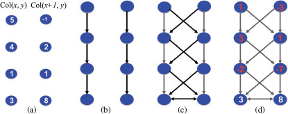
FIGURE 10.4
Illustrating the graph construction for the OSSD problem. The construction is exemplified on two adjacent columns. The surface smoothness parameter Δx = 1. (a) Two adjacent columns of voxels. Each number is the edge-based cost of the corresponding voxel. (b) The intracolumn arcs (black) pointing downward enforce the monotonicity of the sought surface. (c) The intercolumn arcs (black) enforce the surface smoothness constraints. (d) Node costs assignment scheme.

Given any closed set $C \neq \emptyset$ in $G$ , we define a feasible surface S in $ℐ$ , as follows. For each (x, y)-pair, let $C (x, y) \subset C$ be the set of nodes on the column Col(x, y) of $G$ . Based on the construction of $G$ , it is not hard to see that $C (x, y) \neq \emptyset$ . Let z_h (x, y) be the largest z-coordinate of the nodes in $C (x, y)$ . Define the surface S as S(x, y) = z_h(x, y) for every (x, y)-pair. Figure 10.5 shows an example of recovering a feasible surface from a closed set.

Hence, we can compute a minimum-cost closed set $C^{*} \neq \emptyset$ in $G$ , which specifies an optimal single surface S* in $ℐ$ . However, the minimum closed set $C^{*}$ in G′ can be empty (with a cost zero), and when this is the case, $C^{*} = \emptyset$ gives little useful information on recovering the surface. Fortunately, our careful construction of $G$ still enables us to overcome this difficulty. If the minimum closed set in $G$ is empty, then it implies that the cost of every nonempty closed set in $G$ is nonnegative. We want to do a transformation to reduce the cost of every closed set in $G$ by a constant to make sure that at least one is of negative cost. To do so, we investigate a special closed set $C_{0}$ consisting of the “bottom” nodes of all columns in $G$ , that is, $C_{0} = {υ (x, y, 0) | 0 \leq x < X, 0 \leq y < Y}$ . The construction of the graph $G$ indicates that $C_{0}$ is a closed set and is a subset of any nonempty closed set in $G$ . Hence, to obtain a minimum nonempty closed set in $G$ , we do the following: Let M be the total cost of nodes in $C_{0}$ ; if M > 0, pick an arbitrary node $υ (x_{0}, y_{0}, 0) \in C_{0}$ and assign a new weight w(x₀, y₀, 0) − M − 1 to υ(x₀, y₀, 0) (Figure 10.6(a)). We call this a translation operation on $G$ . Thus, the total cost of the closed set $C_{0}$ (after a translation operation on $G$ ) is negative. Since $C_{0}$ is a subset of any non-empty closed set in $G$ , the cost of any nonempty closed set is reduced by (M + 1). Hence, the minimum-cost nonempty closed set in $G$ is not changed after the translation operation, and it cannot be empty. Then, we can simply find a minimum closed set $C^{*}$ in $G$ after performing a translation operation on $G$ . $C^{*}$ is a minimum-cost nonempty closed set in $G$ before the translation.

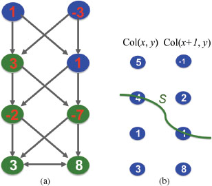
FIGURE 10.5
Illustrating the recovery of a feasible surface from a closed set. (a) shows a closed set in the constructed graph in Figure 10.4(d), which consists of all green nodes. The surface specified by the closed set in (a) is shown in (b).

As in [14, 15, 2, 16], we find a minimum-cost closed set $C^{*} \neq \emptyset$ in $G$ by formulating it as computing a minimum s-t cut in a weighted directed graph $G^{'}$ transformed from $G$ . Let $V^{+}$ and $V^{-}$ denote the set of nodes in $G$ with nonnegative and negative costs, respectively. Define a new directed graph $G_{s t} = (V \cup {s, t}, ℰ \cup ℰ_{s t})$ . The node set of $G_{s t}$ is the node set $V$ of $G$ plus a source s and a sink t. The arc set of $G_{s t}$ is the arc set $ℰ$ of $G$ plus a new arc set $ℰ_{s t}$ . $ℰ_{s t}$ consists of the following arcs: The source s is connected to each node $υ \in V^{-}$ by an arc of cost −w(υ); every node $υ \in V^{+}$ is connected to the sink t by an arc of cost w(υ) (Figure 10.6(a)). Let $(A, \bar{A})$ denote a finite-cost s-t cut in $G_{s t}$ with s ∈ A and $t \in \bar{A}$ , and $C (A, \bar{A})$ denote the total cost of the cut. Note that the arcs in the cut $(A, \bar{A})$ are either in $(A \cap V^{+}, t)$ or in $(s, \bar{A} \cap V^{-})$ . Let w(V′) denote the total cost of nodes in a subset $V^{'} \subseteq V$ .

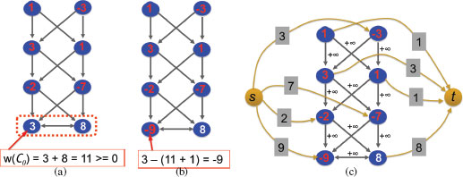
FIGURE 10.6
Illustrating the computation of a minimum-cost nonempty closed set. (a) The “bottom” nodes of all columns forms a minimal closed set which is a subset of any nonempty closed set of the graph in Figure 10.4(d). (b) Performing a translation operation on the graph in (a). (b) The constructed s-t graph for computing a minimum-cost nonempty closed set.

$\begin{array}{l} C (A, \bar{A}) = & \sum_{υ \in \bar{A} \cap V^{-}} (- w (υ)) + \sum_{υ \in A \cap V^{+}} w (υ) \\ = & \sum_{υ \in V^{-}} (- w (υ)) - \sum_{υ \in A \cap V^{-}} (- w (υ)) + \sum_{υ \in A \cap V^{+}} w (υ) \\ = & - w (V^{-}) + \sum_{υ \in A} w (υ) \end{array}$

(10.3)

Note that the term −w(V⁻) is fixed and is the sum over all nodes with negative costs in $G$ . The term $\sum_{υ \in S} w (υ)$ is the total cost of all nodes in the source set A of the cut $(A, \bar{A})$ . But, A − {s} is a closed set in $G$ [14, 15]. Thus, the cost of a cut $(A, \bar{A})$ in G_st and the cost of the corresponding closed set in $G$ differ by a constant, and the source set of a minimum cut in G_st corresponds to a minimum-cost closed set in $G$ .

Therefore, the minimum s-t cut in $G_{s t}$ defines a minimum-cost closed set $C^{*}$ in $G$ , which can be used to specify an optimal single surface S* in $ℐ$ .

10.3.3 Optimal Multiple Surface Detection

This section presents the algorithm for solving the optimal multiple surface detection (OMSD) problem, i.e., simultaneous detection of λ > 1 interrelated surfaces in a 3-D image $ℐ$ such that the total cost of the λ surfaces defined in Equation 10.1 is minimized [3, 16]. In addition to the intralayer self-closure structure for each single surface, we further explore the interlayer self-closure structure of the pairwise interacting surfaces, which again enables us to model the OMSD problem as a minimum-cost closed set problem.

10.3.3.1 Overview of the OMSD Algorithm

The OMSD algorithm is based on a sophisticated graph transformation scheme, which enables us to simultaneously identify λ > 1 optimal interrelated net surfaces as a whole by computing a minimum-cost closed set in a weighted directed graph $G$ that we transform from $ℐ$ . The algorithm uses the following three main steps.

Step 1: Graph Construction. Build a node-weighted directed graph $G = (V, ℰ)$ , which contains λ node-disjoint subgraphs $G_{i} = (V_{i}, ℰ_{i})$ . Each subgraph $G_{i}$ is used to search for the i-th surface in $ℐ$ . The separation constraints of the surfaces are enforced by introducing a subset of directed arcs between any two adjacent subgraphs, $G_{i}$ and $G_{i + 1} (i = 1, 2, \dots, λ - 1)$ . The construction of the graph $G$ (see Section 10.3.3.3) hinges on the self-closure structure exploited in Section 10.3.3.2.

Step 2: Computing a Minimum-Cost Closed Set. Compute a minimum-cost nonempty closed set $C^{*}$ in $G$ , which can be done by formulating it as computing a minimum s-t cut in an edge-weighted directed graph transformed from $G$ .

Step 3: Surfaces Reconstruction. The optimal set of λ surfaces is reconstructed from the minimum-cost closed set $C^{*}$ with each surface being specified by $C^{*} \cap V_{i}$ .

10.3.3.2 The self-closure structure of the OMSD Problem

Assume that $S = {S_{1}, S_{2}, \dots, S_{λ}}$ is a feasible set of λ surfaces in $ℐ$ with S_i+1 being “on top” of S_i. For each pair of the sought surfaces, S_i and S_i+1, two parameters $δ_{i}^{l} \geq 0$ and $δ_{i}^{u} \geq 0$ ¹ are used to specify the surface separation constraint (note that we may define the separation constraint between any pair of the surfaces in $S$ ). First, consider each individual surface $S_{i} \in S$ . Recall that Lw(S_i) denotes the subset of all voxels of $ℐ$ that are on or below S_i. As in Section 10.3.2.1, we observe that each Lw(S_i) has the intralayer self-closure structure.

However, the task here is more involved since the λ surfaces in $S$ are interrelated. The following observation reveals the common essential structure between the smoothness and the separation constraints, leading us to further examine the closure structure between the Lw(S_i)’s. We may view the 3-D image $ℐ$ as a set of X 2-D slices embedded in the yz-plane. Thus, a feasible surface S of $ℐ$ is decomposed into X z-monotone curves with each in a 2-D slice. We observe that each feasible z-monotone curve is subjective to the smoothness constraint in the corresponding slice, and any pair of adjacent z-monotone curves expresses to meet the analogical separation constraints. This observation suggests that the surface separation constraint in a d-D image may be viewed as the surface smoothness constraint in the (d + 1)-D image consisting of the stack of a sequence of λ d-D images. Hence, we intend to map the detection of λ optimal surfaces in d-D to the problem of finding a single optimal surface in (d+1)-D.

To distinguish the self-closure structures, we define below the upstream and downstream voxels of any voxel $ℐ (x, y, z)$ in $ℐ$ for the given surface separation parameters $δ_{i}^{l}$ and $δ_{i}^{u}$ : if $ℐ (x, y, z) \in S_{i}$ , then the i-th upstream (respectively, downstream) voxel of $ℐ (x, y, z)$ is the voxel on column Col(x, y) with the smallest z-coordinate that can be on S_i+1 (respectively, S_i−1). More precisely, for every voxel $ℐ (x, y, z)$ and 1 ≤ i < λ (respectively, 1 < i ≤ λ), the i-th upstream (respectively, downstream) voxel of $ℐ (x, y, z)$ is $ℐ (x, y, z + δ_{i}^{l})$ (respectively, $ℐ (x, y, \max {0, z - δ_{i - 1}^{u}})$ ) if $z + δ_{i}^{l} < Z$ (respectively, $z - δ_{i - 1}^{l} \geq 0$ ). Consider any voxel $ℐ (x, y, z) \in L w (S_{i})$ . Since z ≤ S_i(x, y), the i-th upstream voxel of $ℐ (x, y, S_{i} (x, y))$ is “above” the i-th upstream voxel of $ℐ (x, y, z)$ (i.e., $S_{i} (x, y) + δ_{i}^{l} \geq z + δ_{i}^{l}$ ). In the meanwhile, $S_{i + 1} (x, y) \geq S_{i} (x, y) + δ_{i}^{l}$ (by the definition of the i-th upstream voxel). Hence, the i-th upstream voxel of $ℐ (x, y, z)$ , $ℐ (x, y, z + δ_{i}^{l})$ , is in Lw(S_i+1). Using a similar argument, the i-th downstream voxel of $ℐ (x, y, z)$ , $ℐ (x, y, \max {0, z - δ_{i - 1}^{u}})$ , is in Lw(S_i−1). Thus, we have the following interlayer self-closure structure of Lw(S_i)’s: Given any set $S$ of λ feasible surfaces in $I$ , the i-th upstream (respectively, downstream) voxel of each voxel in Lw(S_i) is in Lw(S_i+1) (respectively, Lw(S_i−1)), for every 1 ≤ i < λ (respectively, 1 < i ≤ λ).

Both the intralayer and interlayer self-closure structures together bridge the OMSD problem and the minimum closed set problem. Instead of directly searching for an optimal set of λ surfaces, $S^{*} = {S_{1}^{*}, S_{2}^{*}, \dots, S_{λ}^{*}}$ , we intend to find λ optimal subsets of voxels in $ℐ$ , $Lw (S_{1}^{*}) \subset Lw (S_{2}^{*}) \subset \dots \subset Lw (S_{λ}^{*})$ , such that each $Lw (S_{i}^{*})$ uniquely defines a surface $S_{i}^{*} \in S^{*}$ .

10.3.3.3 The Graph Transformation Scheme for the OMSD Problem

This section presents the construction of the node-weighted directed graph $G = (V, ℰ)$ , enabling us to simultaneously identify an optimal set of λ > 1 interrelated surfaces as a whole by computing a minimum-cost closed set. An example of the construction is shown in Figure 10.7.

The graph $G$ contains λ node-disjoint subgraphs ${G_{i} = (V_{i}, ℰ_{i}) | i = 1, 2, \dots, λ}$ ; each $G_{i}$ is for the search of the i-th surface S_i. $V = \cap_{i = 1}^{λ} V_{i}$ and $ℰ = \cap_{i = 1}^{λ} ℰ_{i} \cup ℰ_{s}$ . The surface separation constraints between any two consecutive surfaces S_i and S_i+1 are enforced in $G$ by a subset of edges in $ℰ_{s}$ , which connect the corresponding subgraphs $G_{i}$ and $G_{i + 1}$ . Each subgraph $G_{i}$ is constructed in the same way as in Section 10.3.2.2 by observing the intralayer self-closure structure of the problem (Figure 10.7(b)).

We then put directed arcs into $ℰ_{s}$ between $G_{i}$ and $G_{i + 1}$ , to enforce the surface separation constraints. From the interlayer self-closure property, if voxel $ℐ (x, y, z) \in S_{i}$ , then its i-th upstream voxel $ℐ (x, y, z + δ_{i}^{l})$ must be on or below the surface S_i+1 (i.e., $ℐ (x, y, z + δ_{i}^{l}) \in Lw (S_{i + 1})$ ). Thus, for each node υ_i(x, y, z) with $z < Z - δ_{i}^{l}$ on the column Col_i(x, y) of $G_{i}$ , a directed arc is put in $ℰ_{s}$ from υ_i(x, y, z) to $υ_{i + 1} (x, y, z + δ_{i}^{l})$ on Col_i+1(x, y) of $G_{i + 1}$ . Intuitively, these arcs ensure that the surface S_i+1 must be at a distance of at least $δ_{i}^{l}$ “above” S_i (i.e., for each (x, y)-pair, $S_{i + 1} (x, y) - S_{i} (x, y) \geq δ_{i}^{l}$ . On the other hand, each node υ_i+1(x, y, z) with $z \geq δ_{i}^{l}$ on Col_i+1(x, y) has a directed arc in $ℰ_{s}$ to υ_i(x, y, z′) on Col_i(x, y) with $z^{'} = \max {0, z - δ_{i}^{u}}$ (note that $ℐ (x, y, z^{'})$ is the (i + 1)-st downstream voxel of $ℐ (x, y, z)$ , making sure that S_i+1 must be at a distance of no larger than $δ_{i}^{u}$ “above” S_i (i.e., for each (x, y)-pair, $S_{i + 1} (x, y) - S_{i} (x, y) \leq δ_{i}^{u}$ . This construction is applied to every pair of the corresponding columns of any two subgraphs $G_{i}$ and $G_{i + 1}$ , for i = 1, 2, …, λ – 1. Figure 10.7(c) shows an example of introducing those intergraph arcs.

Recall that we aim to compute a minimum-cost non-empty closed set in $G$ , which can specify λ optimal surfaces in I. However, the graph $G$ constructed up to this point does not yet work for this purpose. In the graph construction above, one may notice that any node υ_i(x, y, z) with $z \geq Z - δ_{i}^{l}$ has no arc to any node on Col_i+1(x, y), and any node υ_i+1(x, y, z) with $z < δ_{i}^{l}$ has no arc with any node on Col_i(x, y). Each of those nodes of $G$ is called a deficient node. The voxels corresponding to the deficient nodes cannot be on any feasible surface. Thus, those deficient nodes along with their incident arcs are safe to be removed (Figure 10.7(d)). The removal of the deficient nodes may also cause other nodes to be deficient (i.e., their corresponding voxels cannot be on any feasible surface). We need to continue eliminate those new deficient nodes. We simply denote also by $G$ the graph after the deficient node pruning process. Note that in the resulting graph $G$ if any column Col_i(x, y) = ∅, then there is no feasible solution to the OMSD problem. In the rest of this section, we assume that the OMSD problem has feasible solutions. Then, for every (x, y)-pair and i = 1, 2, …, λ, let $z_{i}^{bot} (x, y)$ and $z_{i}^{top} (x, y)$ be the smallest and largest z-coordinates of the nodes on the column Col_i(x, y) of G_i, respectively. The deficient node pruning process may remove some useful arcs whose ending nodes need to be changed. For any node υ_i(x, y, z) with $z < z_{i}^{bot} (x, y)$ in $G$ before the pruning process, if it has an incoming arc, the ending node of the arc needs to be changed to the node $υ_{i} (x, y, z_{i}^{bot} (x, y))$ in $G$ after the pruning process (Figure 10.7(d)).

We next further assign a cost w(·) to each node in $G$ , as follows. For every (x, y)-pair, the cost of the node υ_i(x, y, z) is assigned as w_i(x, y, z), with

$w_{i} (x, y, z) = {\begin{array}{l} b_{i} (x, y, z) + \sum_{j = 0}^{z} [c_{i - 1} (x, y, j) - c_{i} (x, y, j)] \\ if z = z_{i}^{bot} (x, y), \\ [b_{i} (x, y, z) - b_{i} (x, y, z - 1)] + [c_{i - 1} (x, y, z) - c_{i} (x, y, z)] \\ for z = z_{i}^{bot} (x, y) + 1, \dots, z_{i}^{top} (x, y) . \end{array}$

(10.4)

This completes the construction of $G$ . It takes O(λn) time to construct the graph, which has O(λn) nodes and O(λn) arcs.

10.3.3.4 Computing Optimal Multiple Surfaces for the OMSD Problem

The graph $G$ thus constructed allows us to find an optimal set of λ surfaces in $ℐ$ , by computing a nonempty minimum-cost closed set in $G$ . In order to do that, as in Ref. [16, 3], we can prove the following facts: (1) Any closed set $C \neq \emptyset$ in $G$ defines a set $S$ of λ feasible surfaces {S₁, S₂, …, S_λ} in $ℐ$ ; (2) any set $S = {S_{1}, S_{2}, \dots, S_{λ}}$ of λ feasible surfaces in $ℐ$ corresponds to a closed set $C \neq \emptyset$ in $G$ . Furthermore, we can show that the cost $α (S)$ of $S$ differs by a fixed value from the total cost $w (C)$ of $C$ . Let $C_{i} = C \cap V_{i}$ and denote by $C_{i} (x, y)$ the set of nodes of $C_{i}$ on the column Col_i(x, y) of G_i. Note that if a node $υ_{i} (x, y, z_{c}) \in C_{i} (υ)$ , then all nodes in ${υ_{i} (x, y, z) | υ_{i} (x, y, z) \in {Col}_{i} (x, y), z \leq z_{c}}$ are also in $C_{i} (x, y)$ . Hence, the total node cost of $C_{i} (x, y)$ is $w (C_{i} (x, y)) = \sum_{z = z_{i}^{bot} (x, y)}^{S_{i} (x, y)} w_{i} (x, y, z)$ . Thus, we have

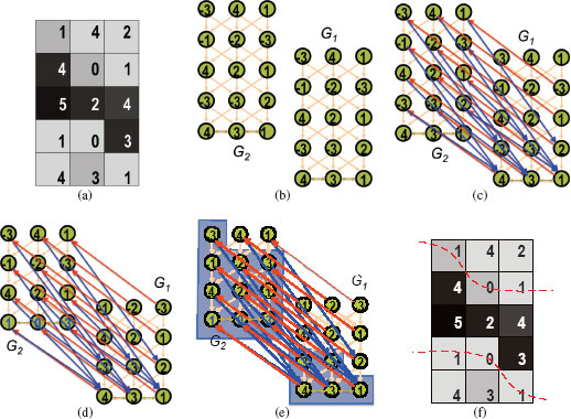
$\begin{array}{l} α (S) = \sum_{i = 1}^{λ} b_{i} (S_{i}) + \sum_{i = 0}^{λ} c_{i} (R_{i}) = \sum_{i = 1}^{λ} \sum_{ℐ (x, y, z) \in S_{i}} b_{i} (x, y, z) + \sum_{i = 0}^{λ} \sum_{ℐ (x, y, z) \in R_{i}} c_{i} (x, y, z) \\ = \sum_{i = 1}^{λ} \sum_{(x, y)} {b_{i} (x, y, 0) + \sum_{z = 1}^{S_{i} (x, y)} [b_{i} (x, y, z) - b_{i} (x, y, z - 1)]} \\ + (\sum_{i = 1}^{λ} \sum_{(x, y)} \sum_{z = 0}^{S_{i} (x, y)} [c_{i} - 1 (x, y, z) - c_{i} (x, y, z)] + \sum_{(x, y)} \sum_{z = 0}^{Z - 1} c_{λ} (x, y, z)) = \\ \sum_{i = 1}^{λ} \sum_{(x, y)} & {\underset{the cost of the "bottom-most" node υ_{i} (x, y, z_{b}) (z_{b} = z_{i}^{bot} (x, y)) of {Col}_{i} (x, y) in G_{i}}{\underset{︸}{(b_{i} (x, y, 0) + \sum_{z = 1}^{z_{i}^{bot} (x, y)} [b_{i} (x, y, z) - b_{i} (x, y, z - 1)] + \sum_{z = 0}^{z_{i}^{bot} (x, y)} [c_{i - 1} (x, y, z) - c_{i} (x, y, z)])}} \\ + \sum_{z = z_{i}^{bot} (x, y) + 1}^{S_{i} (x, y)} \underset{the cost of node υ_{i} (x, y, z) \in {Col}_{i} (x, y)}{\underset{︸}{([b_{i} (x, y, z) - b_{i} (x, y, z - 1)] + [c_{i - 1} (x, y, z) - c_{i} (x, y, z)])}}} \\ + \sum_{(x, y)} \sum_{z = 0}^{Z - 1} c_{λ} (x, y, z) \\ = \sum_{i = 1}^{λ} \sum_{(x, y)} \sum_{z = z_{i}^{bot} (x, y)}^{S_{i} (x, y)} w_{i} (x, y, z) + \sum_{(x, y)} \sum_{z = 0}^{Z - 1} c_{λ} (x, y, z) \\ = \sum_{i = 1}^{λ} \sum_{(x, y)} w_{i} (C_{i} (x, y)) + \sum_{(x, y)} \sum_{z = 0}^{Z - 1} c_{λ} (x, y, z) \\ = w (C) + \sum_{(x, y)} \sum_{z = 0}^{Z - 1} c_{λ} (x, y, z) \end{array}$

(10.5)

FIGURE 10.7
Illustrating the optimal multiple surface detection algorithm. For the purpose of visualization, a 2-D image (a) is used. Only edge-based costs are used and no region-based costs are considered in this example. The number in each pixel is its edge-based cost. Two interacting surfaces are desired to be detected. The surface smoothness parameter is Δx = 1, the minimum surface distance δ^l = 1, and the maximum surface distance δ^u = 3. (b) shows two subgraphs constructed from the image in (a), each is used to search one surface. The introduced arcs (red and blue) shown in (c) to enforce the minimum and maximum distance between two sought surfaces. The topmost row of nodes in G₁ and the bottom-most row of nodes in G₂ may not present on any feasible surface and are removed as in (d). (e) shows a minimum-cost nonempty closed set in $G$ , which consists of all nodes in the blue boxes. The recovered two surfaces are shown in (f).

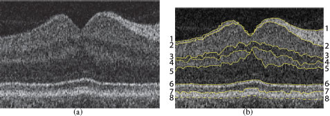
FIGURE 10.8
Segmentation of multiple (8) surfaces on one slice from spectral-domain 3-D OCT volume. Note the fovea location “dip” in the middle of the image slice.

Note that the term $\sum_{(x, y)} \sum_{z = 0}^{Z - 1} c_{λ} (x, y, z)$ is fixed and is the total sum of the λ-th in-region costs of all voxels in $ℐ$ . Consequently, a minimum-cost nonempty closed set $C^{*}$ in $G$ (Figure 10.7(e)), which can be computed as in Section 10.3.2.3, can specify an optimal set $S^{*}$ of λ surfaces ${S_{1}^{*}, S_{2}^{*}, \dots, S_{λ}^{*}}$ in $ℐ$ . Each $S_{i}^{*}$ is specified by $C^{*} \cap V_{i}$ as in Section 10.3.2.3 (Figure 10.7(f)).

10.3.4 Optimal Surface Detection with Convex Priors

Up to this point, in our optimal layered graph search model, the node weights in a graph represent the desired segmentation properties such as edge- and region-based image costs, and the desired surface smoothness is hardwired as connectedness of neighboring columns. This representation is limiting the ability to incorporate a broader variety of a priori knowledge in the segmentation process. The connectedness of one voxel to the voxels of its neighboring columns is basically of equal importance in our current model, which prevents us from fully utilizing image edge information as well as from fully taking advantage of shape priors. In some applications, one may prefer to detect surfaces with certain configurations or shapes. For example, the fovea in macular OCT images (Figure 10.8) has a specific shape, the preference of which may be incorporated in the optimization using a weighted agreement between the potential surface solution and the expected shape. In addition, the hardwired smoothness constraints may oversmooth the target surfaces, which makes it difficult to capture their abrupt changes. One way to alleviate this drawback is to use varying smoothness parameters obtained from a training set. It worked quite well in a retinal OCT segmentation as reported in [17]. However, that approach applies only if the dual shape–location dependency is consistent, which is fortunately satisfied in retinal OCT.

To obtain a generally applicable approach, we utilize the weights of both graph nodes and arcs to represent the desired segmentation properties for optimal single- and multiple-surface segmentation, which can incorporate a wide spectrum of constraints into the problem formulation. Let Γ = [0..X − 1] × [0..Y – 1] denote the grid domain of image $ℐ$ . For optimal surface detection, in addition to requiring each surface S to satisfy the hard smoothness constraints as in Section 10.3.1, we introduce into the objective function a soft smoothness a priori shape compliance energy term $ℰ_{smooth} (S)$ on the grid domain Γ for each surface S, with $ℰ_{smooth} (S) = \int_{Γ} ϕ (\nabla S)$ , where ϕ is a smoothness penalty function, for instance, penalizing the first derivatives of the grid Γ deformation. We consider a discrete approximation of $ℰ_{smooth} (S)$ extended by the piecewise property. Assume that $N$ is a given neighborhood system on Γ. For any p(x, y) ∈ Γ, let S(p) denote the z-coordinate of the voxel $ℐ (x, y, z)$ on the surface S. Then, the discrete a priori shape compliance smoothness energy $ℰ_{smooth} (S)$ can be expressed as $\sum_{(p, q) \in N} f_{p, q} (| S (p) - S (q) |)$ , where f_{p, q} is a nondecreasing function associated with two neighboring columns of p and q that penalizes the shape changes of S on p and q. The node-weights are assigned as in our current model to reflect the desired segmentation properties. The enhanced optimal surface detection (EOSD) problem seeks to find a feasible set $S$ of λ surfaces in $ℐ$ such that (1) each individual surface satisfies the hard smoothness constraints; (2) each pair of the surfaces satisfies the surface separation constraints; and (3) the cost $α (S)$ induced by $S$ , with

$\begin{array}{l} α (S) & = \underset{edge term}{\underset{︸}{\sum_{i = 1}^{λ} \sum_{ℐ (x, y, z) \in S_{i}} b_{i} (x, y, z)}} + \underset{region term}{\underset{︸}{\sum_{i = 0}^{λ} \sum_{ℐ (x, y, z) \in R_{i}} c_{i} (x, y, z)}} \\ + \underset{smoothness shape compliance term}{\underset{︸}{\sum_{i = 1}^{λ} \sum_{(p, q) \in N} f_{p, q}^{(i)} (| S_{i} (p) - S_{i} (q) |),}} \end{array}$

(10.6)

is minimized. The objective function $α (S)$ actually is that for the OSD problem (Equation (10.1) in Section 10.3.1) plus the total smoothness a priori shape compliance energy of λ surfaces in $S$ (i.e., $\sum_{i = 1}^{λ} ℰ_{smooth} (S_{i})$ .

The most related problem is the metric labeling problem in computer science or called the Markov Random Field (MRF) optimization problem in computer vision. Our EOSD problem is a substantial generalization of the metric labeling problem, in which λ = 1 and no region term is involved. The metric labeling problem captures a broad range of classification problems where the quality of a labeling depends on the pairwise relations between the underlying set of objects, such as image restoration [18, 19], image segmentation [20, 21, 22, 23], visual correspondence [24, 25], and deformable registration [26]. After being introduced by Kleinberg and Tardos [27], it has been studied extensively in theoretical computer science [28, 29, 30, 31]. The best-known approximation algorithm for the problem is an O(log L) (L is the number of labels, or in our case, L = Z) [30, 27] and has no $Ω (\sqrt{\log L})$ ) approximation unless NP has quasi-polynomial time algorithms [29]. Due to the application nature of the problem, researchers in image processing and computer vision have also developed a variety of good heuristics that use classical combinatorial optimization techniques, such as network flow and local search (e.g., [18, 32, 21, 20, 24, 33]), for solving some special cases of the metric labeling problem.

Due to the NP-hardness of the metric labeling problem, the EOSD problem is NP-hard fornonconvex smoothness penalty functions. In this section, we focus on convex smoothness penalty functions (i.e., $f_{p, q}^{(i)} (\cdot)$ is a convex and nondecreasing function) that are widely used in medical image processing and in Markov Random Fields. The convex metric labeling problem is known to be polynomially solvable (e.g., [2, 33, 34]). Wu and Chen studied a more general case in [2] than both Ahuja et al. [34] and Ishikawa [33] in the sense that they considered nonuniform connectivity between columns. To solve the EOSD problem with convex smoothness penalty functions (convex EOSD, for short), we extend the technique developed for solving the convex metric labeling problem (in which smoothness penalty functions are convex) while incorporating the OMSD algorithm presented in Section 10.3.3 [35]. We reduce the problem to computing a minimum-cost s-excess set in a directed graph. Instead of forcing no arc (directed graph edge) leaving the sought node set, the minimum s-excess problem [2, 34] charges a penalty onto each arc leaving the set (i.e., the tail of the arc is in the set, while the head is not), which can be solved by using a minimum s-t cut algorithm.

10.3.4.1 The Graph Transformation Scheme for the Convex EOSD Problem

The graph $G = (V, ℰ)$ consists of λ node-disjoint subgraphs ${G_{i} = (V_{i}, ℰ_{i}) | i = 1, 2, \dots, λ}$ ; each $G_{i}$ is for the search of the i-th surface S_i, as constructed in Section 10.3.2. We thus enforce in $G$ both surface smoothness and surface separation constraints and incorporate the edge term and the region term of Equation 10.6.

The remaining problem is how to incorporate the soft smoothness a priori shape compliance term in Equation 10.6. Note that the minimum s-excess problem can be solved by computing a minimum s-t cut. Essentially, we need to “distribute” the cost f_p,q(|S(p) − S(q)|) to the corresponding cut between the columns in $G$ corresponding to the columns p and q in $ℐ$ . Two intertwined questions need to be answered: how to put arcs between two adjacent columns, and how to assign a nonnegative cost to each arc (negative arc costs make the computation of a minimum s-excess computationally intractable). Fortunately, the (discrete equivalent of) second derivative of $f_{p, q}^{(i)} (\cdot)$ defined as in Equation 10.7, has the desired features that $f^{″}_{p, q}^{(i)} (h) \geq 0$ for h = 0, 1, 2, …, Δx − 1(Δ_y − 1).

$\begin{array}{l} f^{″}_{p, q}^{(i)} (0) & = f_{p, q}^{(i)} (1) - f_{p, q}^{(i)} (0) \\ f^{″}_{p, q}^{(i)} (h) & = [f_{p, q}^{(i)} (h + 1) - f_{p, q}^{(i)} (h)] - [f_{p, q}^{(i)} (h) - f_{p, q}^{(i)} (h - 1)], \\ h = 1, 2, \dots, Δ_{x} - 1 (Δ_{y} - 1) . \end{array}$

(10.7)

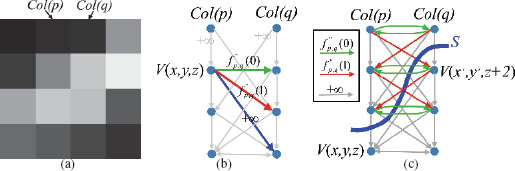
FIGURE 10.9
Graph construction for the convex smoothness penalty function. (a) Example of two adjacent columns. The smoothness parameter Δ_x = 2. (b) Weighted arcs introduced for each node V(x, y, z). Gray arcs of weight +∞ reflect the hard smoothness constraints. (c) Weighted arcs are built between nodes corresponding to the two adjacent columns. The feasible surface S cuts the arcs with a total weight of $f_{p, q} (2) = f_{p, q}^{″} (0) + [f_{p, q}^{″} (0) + f_{p, q}^{″} (1)]$ , which determines smoothness shape compliance term of α(S) for the two adjacent columns.

Based on $f^{″}_{p, q}^{(i)} (\cdot)$ , a cost distribution scheme is developed [2, 33, 34] to incorporate the soft smoothness a priori shape compliance term (Figure 10.9). Assume that the surface smoothness parameters are Δx and Δy. For each subgraph $G_{i}$ , we introduce additional intercolumn arcs: for each h = 0, 1, …, Δx − 1 (Δy — 1), υ_i(x, y, z) has an arc to υ_i(x′, y′, z − h) with an arc-weight of $f^{″}_{p, q}^{(i)} (h)$ (Figure 10.9(b)), where p(x, y) and q(x′, y′) are two adjacent columns with |x – x′| + |y – y′| = 1 (note that we consider 4-neighborhood setting). Thus, the size of the graph $G$ is of O(λn) nodes and O((Δx + Δy)λn) arcs.

10.3.4.2 Computing Optimal Multiple Surfaces for the Convex EOSD Problem

In the following, we show that using this construction, the total cost of the arcs that are cut by a feasible surface S_i between two adjacent columns Col(p) and Col(q) equals the shape prior penalty $f_{p, q}^{(i)} (| S_{i} (p) - S_{i} (q) |)$ . Without loss of generality, assume that $f_{p, q}^{(i)} (0) = 0$ (otherwise, we can subtract $f_{p, q}^{(i)} (0)$ from the cost of each arc from Col(p) to Col(q) without affecting the optimal solution). Let z_p = S_i(p) and z_q = S_i(q). We next only consider the case that z_p ≥ z_q (the case z_p ≤ z_q can be symmetrically the same). If z_p = z_q, S_i does not cut any inter-column arc between Col(p) to Col(q). Thus, the induced penalty is zero, which is the same as the cost $f_{p, q}^{(i)} (0)$ . We now consider the case with z_p > z_q. For each z with z_q < z ≤ z_p, υ_i(x, y, z) has a directed arc in $G_{i}$ to each node υ_i(x′, y′, zz) for z_q < zz ≤ z, with a cost of $f^{″}_{p, q}^{(i)} (z - z z)$ . Below, we list all directed arcs cut by the surface S_i in such a way that each row is for the arcs originating from the same node in Col(p) and each column is for the arcs pointing to the same node in Col(q), as follows:

$\begin{array}{l} (\begin{matrix} υ_{i} (x, y, z_{p}), \\ υ_{i} (x^{'}, y^{'}, z_{p}) \end{matrix}) & (\begin{matrix} υ_{i} (x, y, z_{p}), \\ υ_{i} (x^{'}, y^{'}, z_{p} - 1) \end{matrix}) & \dots, & (\begin{matrix} υ_{i} (x, y, z_{p}), \\ υ_{i} (x^{'}, y^{'}, z_{p} + 1) \end{matrix}) \\ (\begin{matrix} υ_{i} (x, y, z_{p} - 1), \\ υ_{i} (x^{'}, y^{'}, z_{p} - 1) \end{matrix}) & \dots, & (\begin{matrix} υ_{i} (x, y, z_{p} - 1), \\ υ_{i} (x^{'}, y^{'}, z_{p} + 1) \end{matrix}) \\ ⋮ \\ (\begin{matrix} υ_{i} (x, y, z_{p} + 1), \\ υ_{i} (x^{'}, y^{'}, z_{p} + 1) \end{matrix}) \end{array}$

The total cost of those cut arcs between Col(p) and Col(q) equals

$\begin{array}{l} f^{″}_{p, q}^{(i)} (0) + [f^{″}_{p, q}^{(i)} (0) + f^{″}_{p, q}^{(i)} (1)] + \dots + \\ [f^{″}_{p, q}^{(i)} (0) + \dots + f^{″}_{p, q}^{(i)} (z_{p} - z_{q} - 2) + f^{″}_{p, q}^{(i)} (z_{p} - z_{q} - 1)] \\ = & [f_{p, q}^{(i)} (1) - f_{p, q}^{(i)} (0)] + [f_{p, q}^{(i)} (2) - f_{p, q}^{(i)} (1)] + \dots + \\ [f_{p, q}^{(i)} (z_{p} - z_{q}) - f_{p, q}^{(i)} (z_{p} - z_{q} - 1)] \\ = & f_{p, q}^{(i)} (z_{p} - z_{q}) (note that f_{p, q}^{(i)} (0) = 0) \end{array}$

(10.8)

Figure 10.9(c) shows the directed arcs cut by the surface S for the case z_p ≤ z_q.

Hence, we prove that the total cost of the arcs that are cut by a feasible surface S_i between two adjacent columns Col(p) and Col(q) equals the shape prior penalty $f_{p, q}^{(i)} (| S_{i} (p) - S_{i} (q) |)$ .

Then, together with a similar argument in Section 10.3.3, we are able to show the following facts: (1) Any nonempty s-excess set $X$ with a finite cost in $G$ defines λ feasible surfaces in $ℐ$ whose total cost differs from that of $X$ by a fixed value; (2) any set $S$ of λ feasible surfaces in $ℐ$ corresponds to a nonempty s-excess set $X$ in $G$ whose cost differs from that of $S$ by a fixed value. Consequently, a nonempty s-excess set in $G$ with the minimum cost can specify an optimal set of λ surfaces in $ℐ$ while minimizing the energy function (10.6).

A minimum s-excess set in $G$ can be computed by using a minimum s-t cut algorithm, as in [22]. If the minimum s-excess set in $G$ thus obtained is empty, we can first perform on $G$ a translation operation similar to that in Section 10.3.2, and then apply the s-t cut based algorithm to obtain a minimum nonempty s-excess set in $G$ . As in Section 10.3.2, we define a directed graph $G_{s t}$ from $G$ and then compute a minimum s-t cut $(A^{*}, {\bar{A}}^{*})$ in $G_{s t}$ . Then, $X^{*} = A^{*} - {s}$ is the minimum-cost s-excess set in $G$ , which can be used to specify an optimal set of λ surfaces as in Section 10.3.3.

10.3.5 Layered Optimal Graph Image Segmentation for Multiple Objects and Surfaces — LOGISMOS

The optimal graph-based segmentation approach can offer many advantages when employed for multiobject multisurface segmentation. Such a method allows optimally segmenting multiple surfaces that mutually interact within individual objects and/or between objects. Similar to the multisurface case presented above, intrasurface, intersurface, and interobject relationships are represented by context-specific graph arcs.

When segmenting complex shapes, the LOGISMOS approach [4] typically starts with an object presegmentation step the purpose of which is to identify the topology of the desired segmentaation surfaces. Using the presegmentation information, a single graph holding all relationships and surface cost elements is constructed, in which the segmentation of all desired surfaces is performed simultaneously in a single optimization process. While the description given below specifically refers to 3D image segmentation, the LOGISMOS method is fundamentally n-dimensional.

10.3.5.1 Object Pre-segmentation

The LOGISMOS method begins with a coarse presegmentation of the image data, but there is no prescribed method that must be used. The only requirement is that presegmentation yields robust approximate surfaces of the individual objects, having the same (correct) topology as the underlying objects and being sufficiently close to the true surfaces. The definition of “sufficiently close” is problem-specific and needs to be considered in relationship with how the layered graph is constructed from the approximate surfaces. Note that it is frequently sufficient to generate a single presegmented surface per object, even if the object itself exhibits more than one mutually interacting surface of interest. Depending upon the application, level sets, deformable models, active shape/appearance models, or other segmentation techniques can be used to yield object presegmentations.

10.3.5.2 Construction of Object-Specific Graphs

If the object-specific graph is constructed from a result of object presegmentation, the approximate presegmented surface may be meshed and the graph columns constructed as normals to individual mesh faces. The lengths of the columns are then derived from the expected maximum distances between the presegmented approximate surface and the true surface, so that the correct solution can be found within the constructed graph. Maintaining the same graph structure for individual objects, the base graph is formed using the presegmented surface mesh $M$ . V_B is the vertex set on $M$ and E_B is the edge set. A graph column is formed by equally sampling several nodes along the normal direction of a vertex in V_B. The base graph is formed by connecting the bottom nodes by the connection relationship of E_B. In the multiple closed surface detection case, a duplication of the base graph is constructed each time when searching for an additional surface. The duplicated base graphs are connected by undirected arcs to form a new base graph, which ensures that the interacting surfaces can be detected simultaneously. Additional directed intracolumn arcs, intercolumn arcs, and intersurface arcs incorporate surface smoothness Δ and surface separation δ constraints into the graph.

10.3.5.3 Multiobject Interactions

When multiple objects with multiple surfaces of interest are in close apposition, a multiobject graph construction is adopted. This begins with considering pairwise interacting objects, with the connection of the base graphs of these two objects to form a new base graph. Object interaction is frequently local, limited to only some portions of the two objects’ surfaces. Here we will assume that the region of pairwise mutual object interaction is known. A usual requirement may be that surfaces of closely located adjacent objects do not cross each other, that they are at a specific maximum/minimum distance, or similar. Object-interacting surface separation constraints are implemented by adding interobject arcs at the interacting areas. Interobject surface separation constraints are also added to the interacting areas to define the separation requirements that shall be in place between two adjacent objects. The interobject arcs are constructed in the same way as the intersurface arcs. The challenge in this task is that no one-to-one correspondence exists between the base graphs (meshes) of the interacting object pairs. To address this challenge, corresponding columns i and j need to be defined between the interacting objects. The corresponding columns should have the same directions. Considering signed distance offset d between the vertex sets $V_{i}$ and $V_{j}$ of the two objects, interobject arcs $ℰ^{o}$ between two corresponding columns can be defined as:

$\begin{array}{l} ℰ^{o} & = {〈 V_{i} (k), V_{j} (k - d + δ^{l}) 〉 | \forall k : \\ \max (d - δ^{l}, 0) \leq k \leq \min (K - 1 + d - δ^{l}, K - 1)} \\ \cup {〈 V_{j} (k), V_{i} (k + d - δ^{u}) 〉 | \forall k : \\ \max (δ^{u} - d, 0) \leq k \leq \min (K - 1 + d - δ^{u}, K - 1)} \end{array}$

(10.9)

where k is the vertex index number; δ^l and δ^u are interobject separation constraints with δ^l ≤ δ^u.

Nevertheless, it may be difficult to find corresponding columns between two regions of different topology. The approach presented below offers one possible solution. Since more than two objects may be mutually interacting, more than one set of pairwise interactions may coexist in the constructed graph.

10.3.5.4 Electric Lines of Force

Starting with the initial presegmented shapes, a cross-object search direction must be defined for each location along the surface. The presently adopted method for defining corresponding columns via cross-object surface mapping relies upon electric field theory for a robust and general definition of such search direction lines to guarantee nonintersecting character of the search-direction lines [36]. Recall Coulomb’s law from basic physics

$E_{i} = \frac{1}{4 π ε_{0}} \frac{Q}{r^{2}} \hat{r},$

(10.10)

where E_i is the electric field at point i. Q is the charge of point i; r is the distance from point i to the evaluation point; $\hat{r}$ is the unit vector pointing from the point i to the evaluation point. ε₀ is the vacuum permittivity. Since the total electric field E is the sum of E_i’s

$E = \sum_{i} E_{i},$

(10.11)

the electric field has the same direction as the electric line(s) of force (ELF). When an electric field is generated from multiple source points, the electric lines of force exhibit a nonintersection property, which is of major interest in the context of finding corresponding columns.

When computing ELF for a computer generated 3D triangulated surface, the surface is composed of a limited number of vertices that are usually not uniformly distributed. These two observations greatly reduce the effect of charges located in close proximity. To cope with this undesirable effect, a positive charge Q_i is assigned to each vertex υ_i. The value of Q_i is determined by the area sum of triangles t_j where υ_i ∈ t_j. When changing r² to r^m (m > 2), the nonintersection property still holds. The difference is that more distant vertices will be penalized in ELF computing. Therefore, a slightly larger m will increase the robustness of local ELF computation. Discarding the constant term, the electric field is defined as

$\hat{E} = \sum_{i} \frac{\sum_{j} AREA (t_{j})}{r_{i}^{m}} {\hat{r}}_{i},$

(10.12)

where υ_i ∈ t_j and m > 2.

Assuming there is a closed surface in an n-D space, the point having a zero electric field is the solution of equation $\hat{E} = 0$ . In an extreme case, the closed surface will converge to the solution points when searching along the ELF. Except for these points, the nonintersecting ELF will fill the entire space. Since ELF are nonintersecting, it is easy to interpolate ELF at nonvertex locations on a surface. The interpolation can greatly reduce total ELF computation load when upsampling a surface. In 2D, linear interpolation from two neighboring vertices and their corresponding ELF can be implemented. In 3D, use of barycentric coordinates is preferred to interpolate points within triangles.

When a closed surface is used for ELF computation, isoelectric potential surfaces can be found. Except for the solution points $\hat{E} = 0$ , all other points belong to an isoelectric potential surface and the ELF passing through such a point can be easily interpolated. The interpolated ELF intersects the initial closed surface. Consequently, this technique can be used to create connections between a point in space and a closed surface, yielding cross-surface mapping.

10.3.5.5 ELF-Based Cross-Object Surface Mapping

The nonintersection property of ELF is useful to find one-to-one mapping between adjacent objects with different surface topologies. Interrelated ELF of two coupled surfaces can be determined in two steps:

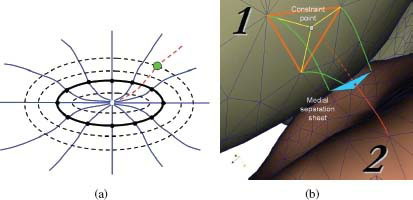
FIGURE 10.10
Cross-object surface mapping by ELF. (a) The ELF (blue lines) are pushed forward from a surface composed of black vertices. The dashed black surfaces indicate the location of isoelectric potential contours. The red-dashed ELF is the traced-back line from a green point to the solid black surface. The traced-back line is computed by interpolating two neighboring pushed-forward ELF. (b) Constraint-point mapping of coupled 3D surfaces is performed in the following 5 steps: (i) Green and red ELF are pushed forward from surface 1 and 2, respectively. (ii) The intersections between the ELF and medial separating sheet form a blue triangle and a red point. (iii) The red point is traced back along dotted red line to surface 1. (iv) When the dotted red line intersects surface 1, it forms a light-blue constraint point on surface 1. (v) The constraint point is connected at surface 1 by yellow edges. Reprinted, with IEEE permission, from [4].

• Push forward—regular ELF path computation using Equation (10.12).

• Trace back—interpolation process to form an ELF path from a point in space to a closed surface as outlined above.

The general idea of mapping two coupled surfaces using ELF includes defining an ELF path using the push forward process, identifying the medial-sheet intersection point on this path, generating a constraint point on the opposite surface, and connecting the constraint point with already existing close vertices on this surface – so called constraint-point mapping [36]. Figure 10.10a shows ELF pushed forward from a surface and traced back from a point to that surface. Figure 10.10b shows an example of mapping two coupled surfaces in 3D.

Note that each vertex in the object-interaction area can therefore be used to create a constraint point affecting the coupled surface. Importantly, the corresponding pairs of vertices (the original vertex and its constraint point) from two interacting objects in the contact area identified using the ELF are guaranteed to be in a one-to-one relationship and all-to-all mapping, irrespective of surface vertex density. As a result, the desirable property of maintaining the previous surface geometry (e.g., the orange triangle in Figure 10.10b) is preserved. Therefore, the mapping procedure avoids surface regeneration and merging [37] (which is usually difficult) and enhances robustness with respect to local roughness of the surface, when compared with our previously introduced nearest point based mapping techniques [38, 39].

10.3.5.6 Cost Function and Graph Optimization

The resulting segmentation is driven by the cost functions associated with the graph vertices. Design of vertex-associated costs is problem specific, and costs may reflect edge-based, region-based, or combined edge–region image properties as already described above. Same as in the earlier cases, the optimization problem can be converted to finding the minimum nonempty closed set in the modified graph. As a result of such single optimization process, a globally optimal solution provides all segmentation surfaces for all involved interacting objects while satisfying all surface and object interaction constraints.

10.4 Case Studies

10.4.1 Segmentation of Retinal Layers in Optical Coherence Tomography Volumes

As a first case study, we consider the task of automatically segmenting multiple retinal layers in spectral-domain optical coherence tomography volumes, as illustrated in Figure 10.8. Segmenting these layers is necessary to quantify changes that occur in these layers as a result of ocular diseases causing blindness, such as glaucoma, diabetic retinopathy, and age-related macular degeneration [40]. Such a task is well suited for utilizing the layer-based graph approach discussed in this chapter as the ultimate goal is to simultaneously define approximately seven-to-eleven layered 3D surfaces within these volumes. Since many of the separating surfaces may seem similar to one another at a local level (e.g., surfaces that indicate a transition from a relatively dark region to a relatively bright region), the ability to simultaneously segment these surfaces in 3D is important, as is possible using the layered graph approach described in this chapter.

10.4.1.1 Graph Structure

As an example of a layered graph segmentation problem, we can assume that in an OCT volume I(x, y, z), we desire to find a set of surfaces, where each surface i can be represented by a function f_i(x, y). Because for every (x, y) location, there is only one z-value on the surface, in constructing the subgraph associated with each surface, we can simply define one column Col(x, y) of nodes for each (x, y) location. This thus results in the set of nodes of the surface subgraph directly corresponding to the voxel locations in the original volume, and we can use a similar notation to index the nodes of the subgraph using N_i(x, y, z) (where x, y, and z correspond to the voxel locations and i corresponds to the surface) as we would index the image volume using I(x, y, z). In finding a simultaneous set of n surfaces, we thus have n subgraphs with nodes N₁(x, y, z), …, N_n(x, y, z). Edges are added between the columns as discussed in general in Section 10.3.2 and 10.3.3 to enforce feasibility constraints (i.e., smoothness and surface separation constraints). Better results can be obtained if we allow this constraints to vary as a function of (x, y) location [41, 42]. Such locally varying constraints can be learned from a training set as described in [41, 42].

While the layered graph approach enables the simultaneous segmentation of all surfaces, further efficiency can be obtained if the surfaces are segmented in groups in a multiresolution fashion [42, 43]. For instance, one might first simultaneously segment a smaller set of the most visible surfaces in a low-resolution representation of the volume, while refining the segmentation (and segmenting more surfaces) more locally in higher resolutions of the volume.

10.4.1.2 Cost Function Design

As reported in [44, 42], segmenting the layers in OCT volumes can benefit from incorporating both edge and regional information into the cost function design (i.e., having both on-surface and in-region costs). In fact, the segmentation of OCT layers was the first application to utilize both of these terms using the graph approach of this chapter. In [45], on-surface costs were defined by computing signed edge terms to favor either a bright-to-dark transition or dark-to-bright-transition, depending on the surface. In-region cost terms were based on fuzzy membership functions in dark, medium, or bright intensity classes so that voxels that most matched the expected intensity range of the region would have the lowest costs. The relative weights of each of these terms was defined based on a training set.

10.4.2 Simultaneous Segmentation of Prostate and Bladder in Computed Tomography Volumes

In the United States, prostate cancer is the most common cancer in men, accounting for about 28% of all newly diagnosed cases [46]. Precise target delineation is critical for a successful 3-D radiotherapy treatment planning for prostate cancer treatment. Automatic segmentation of pelvic structure is of particular difficulty. It involves soft tissues that present a large variability in shape and size. Those soft tissues also have similar intensity and have mutual influence in position and shape. To overcome all these difficulties, both shape prior information and surface context information are incorporated using an arc-weighted graph representation to simultaneously segment prostate and bladder in 3D.

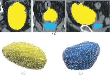
FIGURE 10.11
(a) Presegmentation for bladder (yellow) and prostate (blue) in the transverse (left), coronal (middle) and sagittal (right) views. (b) Triangulated mesh for the bladder. (c) Triangulated mesh for the prostate.

Our method consists of the following steps [47, 35, 48]. First, we obtain a presegmentation of bladder and prostate as the initial shape model, which provides useful information about the topological structures of the target objects (Figure 10.11(a)). A 3-D geodesic active contour method is employed [49] for presegmenting the bladder. The mean shape of the prostate from the training datasets is simply fitted to the never-before seen CT images using a rigid transform. Two triangulated meshes M₁ (V₁, E₁) and M₂(V₂, E₂) are built for the bladder and prostate based on the shape model, respectively (Figure 10.11(b),(c)). Based on these two triangulated meshes, the arc-weighted graph is constructed using the method described in Section 10.3.4. Specifically, two weighted subgraphs $G_{i}$ are built from the mesh M_i as follows. For each vertex υ_i ∈ V_i, a column of K nodes is created in $G_{i}$ . The positions of nodes reflect the positions of corresponding voxels in the image domain. The length of the column is set according to the required search range. The number of nodes K on each column is determined by the required resolution. The direction of the column is set as the triangle normal. The feasible surface S_i in the graph $G_{i}$ is defined as the surface containing exactly one node in each column. To avoid the overlap of two target surfaces, a “partially interacting area” is defined according to the distance between two meshes, which indicates that the two target surfaces may mutually interact each other at that area. To model the interaction relation, the two graphs $G_{1}$ and $G_{2}$ “share” some common node columns in that partially interacting area, and the target surfaces S₁ and S₂ both cut those columns, as shown in Figure 10.12.

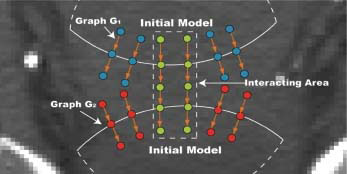
FIGURE 10.12
Graph construction for mutually interacting objects. An example 2-D slice is presented. Note that in the interacting region, for each column with green nodes, there actually exists two columns with the same position, one for Graph $G_{1}$ , one for Graph $G_{2}$ .

Cost function design plays an important role for successful surface detection. In our segmentation, the gradient-based cost function was combined with class uncertainty information for edge-based costs [48]. Given intensity information, the posterior probability that the voxel belongs to the target object is learned from the training set, which is used as the region-based costs. The quadratic shape prior penalty function is obtained from the experiments on the training datasets [48].

The experiments were conducted for simultaneous segmentation of the bladder and the prostate. 3-D CT images from different patients with prostate cancer were used. The image sizes ranged from 80 × 120 × 30 to 190 × 180 × 80 voxels. The image spacing resolution ranged from 0.98 × 0.98 × 3.00 mm³ to 1.60 × 1.60 × 3.00 mm³. Out of 21 volumes, 8 were randomly selected as the training data and our segmentation was performed on the remaining 13 datasets.

For quantitative validation, the result was compared with the expert-defined manual contours. For volumetric error measurement, the Dice similarity coefficient (DSC) was computed using $D = 2 | V_{m} \cap V_{c} | / (| V_{m} | + | V_{c} |)$ , where V_m denotes the manual volumetric result and V_c denotes the computed result. For surface distance error, both mean and the maximum unsigned surface distance error were computed for the bladder and the prostate surfaces between the computed result and the manual delineation. The result is shown in Table 10.1.

For visual performance assessment, the illustrative result with both computed contours and manual contours is displayed in Figure 10.13(a). The 3-D representation was shown in Figure 10.13(d).

Surface	DSC	Mean (mm)	Maximum (mm)
Prostate	0.797	1.01 ± 0.94	5.46 ± 0.96
Bladder	0.900	0.99 ± 0.77	5.88 ± 1.29

TABLE 10.1
Overall quantitative results. Mean ± SD in mm for the unsigned surface distance error.

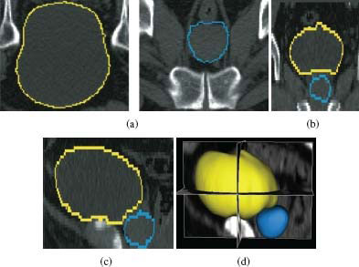
FIGURE 10.13
The bladder (yellow) and the prostate (blue) segmentation results. (a) Transverse view. (b) Coronal view. (c) Sagittal view. (d) 3-D representation of the bladder (yellow) and the prostate (blue).

10.4.3 Cartilage and Bone Segmentation in the Knee Joint

Section 10.3.5 introduced our LOGISMOS method for multiobject, multisurface segmentation. Here we demonstrate its functionality on a knee bone/cartilage segmentation example. In this orthopedic application, a typical scenario includes the need to segment surfaces of the periosteal and subchondral bone and of the overlying articular cartilage from MRI scans with high accuracy and in a globally consistent manner (Figure 10.14).

Three bones articulate in the knee joint: the femur, the tibia, and the patella. Each of these bones is partly covered by cartilage in regions where individual bone pairs slide over each other during joint movements. For assessment of the knee joint cartilage health, it is necessary to identify six surfaces: femoral bone, femoral cartilage, tibial bone, tibial cartilage, patellar bone, and patellar cartilage. In addition to each connected bone and cartilage surface mutually interacting on a given bone, the bones interact in a pairwise manner – cartilage surfaces of the tibia and femur and of the femur and patella are in close proximity (or in frank contact) for any given knee joint position. Clearly, the problem of simultaneous segmentation of the six surfaces belonging to three interacting objects is well suited for application of the LOGISMOS method.

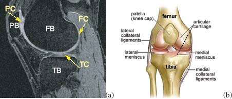
FIGURE 10.14
Human knee. (a) Example MR image of a knee joint — femur, patella, and tibia bones with associated cartilage surfaces are clearly visible. FB = femoral bone, TB = tibial bone, PB = patellar bone, FC = femoral cartilage, TC = tibial cartilage, PC = patellar cartilage. (b) Schematic view of knee anatomy; adapted from [50]. Reprinted, with IEEE permission, from [4].

10.4.3.1 Bone Presegmentation

Figure 10.15 shows the flowchart of our approach [4]. As the first step, the volume of interest (VOI) of each bone, together with its associated cartilage, is identified using an AdaBoost classification approach in 3D MR images. Three VOIs per knee joint image result within which the individual bones (femur, tibia, patella) are located.

After localizing the object VOIs, approximate surfaces of the individual bones must be obtained by first roughly fitting the mean bone shape models directly to the automatically identified VOIs (upper panels of Figure 10.15b). A single surface detection graph was constructed based on the fitted mean shapes – graph columns were built along nonintersecting electric lines of force to increase the robustness of the graph construction (Section 10.3.5.4). The surface costs were associated with each graph node based on the inverted surface likelihood probabilities provided by the random forest classifiers. After repeating this step iteratively until convergence (usually 3–5 iterations were needed), the approximate surfaces of each bone were automatically identified, without considering any bone-to-bone context, see lower panel of Figure 10.15b.

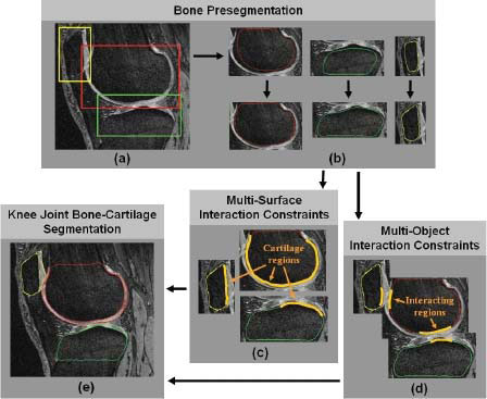
FIGURE 10.15
The flowchart of LOGISMOS-based segmentation of articular cartilage for all bones in the knee joint. (a) Detection of bone volumes of interest using AdaBoost approach. (b) Approximate bone segmentation using single-surface graph search. (c) Generation of multisurface interaction constraints. (d) Construction of multiobject interaction constraints. (e) LOGISMOS-based simultaneous segmentation of 6 bone & cartilage surfaces in 3D. Reprinted, with IEEE permission, from [4].

10.4.3.2 Multisurface Interaction Constraints

Image locations adjacent to and outside of the bone may belong to cartilage, meniscus, synovial fluid, or other tissue, and they thus exhibit different image appearance (Figure 10.15c). Since the cartilage generally covers only those parts of the respective bones which may articulate with another bone, two surfaces (cartilage and bone) are defined only at those locations, while single (bone) surfaces are to be detected in noncartilage regions. To facilitate a topologically robust problem definition across a variety of joint shapes and cartilage disease stages, two surfaces are detected for each bone, and the single–double surface topology differentiation reduces into differentiation of zero and nonzero distances between the two surfaces. In this respect, the noncartilage regions along the external bone surface were identified as regions in which zero distance between the two surfaces was enforced so that the two surfaces collapsed onto each other, effectively forming a single bone surface. In the cartilage regions, the zero-distance rule was not enforced, providing for both a subchondral bone and articular cartilage surface segmentation.

10.4.3.3 Multiobject Interaction Constraints

In addition to dual-surface segmentation that must be performed for each individual bone, the bones of the joint interact in the sense that cartilage surfaces from adjacent bones cannot intersect each other, cartilage and bone surfaces must coincide at the articular margin, the maximum anatomically feasible cartilage thickness shall be observed, etc. The regions in which adjacent cartilage surfaces come into contact are considered the interacting regions (Figure 10.15d). In the knee, such interacting regions exist between the tibia and the femur (tibiofemoral joint) and between the patella and the femur (patellofemoral joint). To automatically find these interacting regions, an isodistance medial separation sheet is identified in the global coordinate system midway between adjacent presegmented bone surfaces. If a vertex is located on an initial surface while having a search direction intersecting the sheet, the vertex is identified as belonging to the region of surface interaction. The separation sheet can be identified using signed distance maps even if the initial surfaces intersect. Following the ELF approach described above, one-to-one and all-to-all corresponding pairs are generated between femur–tibia contact area as well as femur–patella contact area by constraint-point mapping technique. The corresponding pairs and their ELF connections are used for interobject graph link construction [38, 39].

10.4.3.4 Knee Joint Bone–Cartilage Segmentation

After completion of the above steps, the segmentation of multiple surfaces of multiple mutually interacting objects is performed simultaneously and globally optimally subject to the interaction constraints (Figure 10.15e). Specifically, double surface segmentation graphs were constructed individually for each bone using that bone’s initial surface. The three double surface graphs were further connected by interobject graph arcs between the corresponding columns identified during the previous step as belonging to the region of close-contact object interaction. The minimum distance between the interacting cartilage surfaces from adjacent bones was set to zero to avoid cartilage overlap.

10.4.3.5 Knee Joint Bone/Cartilage Segmentation

Our LOGISMOS method was applied to bone/cartilage segmentation of 60 randomly selected knee MR images from the publicly available Osteoarthritis Initiative (OAI) database, which is available for public access at http://www.oai.ucsf.edu/. The MR images used were acquired with a 3T scanner following a standardized procedure. A sagittal 3D dual-echo steady state (DESS) sequence with water excitation and the following imaging parameters: image stack of 384× 384 × 160 voxels, with voxel size of 0.365 × 0.365 × 0.70 mm.

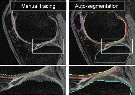
FIGURE 10.16
MR image segmentation of a knee joint – a single contact-area slice from a 3D MR dataset is shown. Segmentation of all six surfaces was performed simultaneously in 3D. (left) Original image data with expert-tracing overlaid. (right) Computer segmentation result. Note that the double-line boundary of tibial bone is caused by intersecting the segmented 3D surface with the image plane. Reprinted, with IEEE permission, from [4].

Figure 10.16 shows an example of a knee joint contact area slice from the 3D MR dataset. Note the contact between the femoral and tibial cartilage surfaces, as well as the contact between the femoral and patellar cartilage surfaces. Furthermore, there is an area of high-intensity synovial fluid adjacent to the femoral cartilage that is not part of the cartilage tissue and should not be segmented as such. The right panel of Figure 10.16 shows the resulting segmentation demonstrating very good delineation of all six segmented surfaces and correct exclusion of the synovial fluid from the cartilage surface segmentations. Since the segmentations are performed simultaneously for all six bone and cartilage surfaces in the 3D space, computer segmentation directly yields the 3D cartilage thickness for all bone surface locations. Typical segmentation results are given in Figure 10.17.

The signed and unsigned surface positioning errors of the obtained cartilage segmentations were quantitatively measured over the cartilage regions. The average signed surface positioning errors for the six detected surfaces ranged from 0.04 to 0.16 mm, while the average unsigned surface positioning error ranged from 0.22 to 0.53 mm. The close-to-zero signed positioning errors attest to a small bias of surface detection. The unsigned positioning errors show that the local fluctuations around the correct location are much smaller than the longest face of MR image voxels (0.70 mm). Our results therefore achieved virtually no surface positioning bias and subvoxel local accuracy for each of the six detected surfaces.

When assessing the performance using Dice coefficients (DSC), the obtained DSC values were 0.84, 0.80 and 0.80, for the femoral, tibial, and patellar cartilage surfaces, respectively.

10.5 Conclusion

The presented framework for simultaneous optimal segmentation of single and multiple surfaces possibly belonging to multiple objects is very powerful. The method can be directly extended to n-D, and the intersurface or interobject relationships can include higher-dimensional interactions, e.g., mutual object motion, interactive shape changes over time, and similar. Overall, the described method is general and useful for a broad range of applications.

10.6 Acknowledgments

This work was supported, in part, by NIH grants R01–EB004640, K25–CA123112, R44–AR052983, P50 AR055533 and by NSF grants CCF-0830402, CCF-0844765.

The Osteoarthritis Initiative (OAI) is a public–private partnership comprised of five contracts (N01-AR-2-2258; N01-AR-2-2259; N01-AR-2-2260; N01-AR-2-2261; N01-AR-2-2262) funded by the NIH and conducted by the OAI Study Investigators. Private funding partners include Merck Research Laboratories; Novartis Pharmaceuticals Corporation, GlaxoSmithKline; and Pfizer, Inc.

Bibliography

[1] M. Sonka, V. Hlavac, and R. Boyle, Image Processing, Analysis, and Machine Vision (3rd ed.). Thomson Engineering, 2008.

[2] X. Wu and D. Chen, “Optimal net surface problems with applications,” in Proc. 29th International Colloquium on Automata, Languages and Programming (ICALP), ser. Lecture Notes in Computer Science, vol. 2380. Springer, July 2002, pp. 1029–1042.

[3] K. Li, X. Wu, D. Chen, and M. Sonka, “Optimal surface segmentation in volumetric images–a graphtheoretic approach,” IEEE Trans. on Pattern Analysis and Machine Intelligence, vol. 28, no. 1, pp. 119–134, 2006.

[4] Y. Yin, X. Zhang, R. Williams, X. Wu, D. Anderson, and M. Sonka, “LOGISMOS - Layered Optimal Graph Image Segmentation of Multiple Objects and Surfaces: Cartilage segmentation in the knee joints,” IEEE Trans. Medical Imaging, vol. 29, no. 12, pp. 2023 – 2037, 2010.

[5] Y. Boykov and G. Funka-Lea, “Graph cuts and efficient n-d image segmentation,” International Journal of Computer Vision, vol. 70, no. 2, pp. 109–131, 2006.

[6] A. Delong and Y. Boykov, “Globally optimal segmentation of multi-region objects,” in International Conference on Computer Vision (ICCV), Kyoto, Japan, 2009, pp. 285–292.

[7] A. Chakraborty, H. Staib, and J. Duncan, “Deformable boundary finding in medical images by integrating gradient and region information,” IEEE Trans. on Medical Imaging, vol. 15, no. 6, pp. 859–870, 1996.

[8] S. Zhu and A. Yuille, “Region competition: Unifying snakes, region growing, and bayes/mdl for multiband image segmentation,” IEEE Trans. on Pattern Analysis and Machine Intelligence, vol. 18, pp. 884–900, 1996.

[9] A. Yezzi, A. Tsai, and A. Willsky, “A statistical approach to snakes for bimodal and trimodal imagery,” in Proc. of Int. Conf. on Computer Vision (ICCV), Corfu, Greece, 1999, pp. 898–903.

[10] N. Paragios and R. Deriche, “Coupled geodesic active regions for image segmentation: A level set approach,” in Proc. of the European Conference in Computer Vision (ECCV), vol. II, 2001, pp. 224–240.

[11] T. F. Chan and L. A. Vese, “Active contour without edges,” IEEE Trans. Image Processing, vol. 10, pp. 266–277, 2001.

[12] N. Paragios, “A variational approach for the segmentation of the left ventricle in cardiac image analysis,” Int. J. of Computer Vision, vol. 46, no. 3, pp. 223–247, 2002.

[13] Y. Boykov and V. Kolmogorov, “Computing geodesics and minimal surfaces via graph cuts,” in Proc. of Int. Conf. on Computer Vision (ICCV), Nice, France, October 2003, pp. 26–33.

[14] J. Picard, “Maximal closure of a graph and applications to combinatorial problems,” Management Science, vol. 22, pp. 1268–1272, 1976.

[15] D. Hochbaum, “A new-old algorithm for minimum-cut and maximum-flow in closure graphs,” Networks, vol. 37, no. 4, pp. 171–193, 2001.

[16] X. Wu, D. Chen, K. Li, and M. Sonka, “The layered net surface problems in discrete geometry and medical image segmentation,” Int. J. Comput. Geometry Appl., vol. 17, no. 3, pp. 261–296, 2007.

[17] M. K. Haeker, M. D. Abràmoff, X. Wu, R. Kardon, and M. Sonka, “Use of varying constraints in optimal 3-D graph search for segmentation of macular optical coherence tomography images,” in Medical Image Computing and Computer-Assisted Intervention (MICCAI 2007), ser. Lecture Notes in Computer Science, N. Ayache, S. Ourselin, and A. Maeder, Eds., vol. 4791. Berlin/New York: Springer, 2007, pp. 244–251.

[18] Y. Boykov, O. Veksler, and R. Zabih, “Markov Random Fields with efficient approximations,” in Proc. of the IEEE Conf. on Computer Vision and Pattern Recognition, 1998, pp. 648–655.

[19] ——, “Fast approximate energy minimization via graph cuts,” IEEE Trans. on Pattern Analysis and Machine Intelligence, vol. 23, no. 11, pp. 1222–1239, 2001.

[20] H. Ishikawa and D. Geiger, “Segmentation by grouping junctions,” in Proc. of the IEEE Conf. on Computer Vision and Pattern Recognition, Santa Barbara, CA, 1998, pp. 125–131.

[21] D. Greig, B. Porteous, and A. Seheult, “Exact maximum a posteriori estimation for binary image,” J. Roy. Statist. Soc. Ser. B, vol. 51, pp. 271–279, 1989.

[22] D. Hochbaum, “An efficient algorithm for image segmentation, markov randomfields and related problems,” J. of the ACM, vol. 48, pp. 686–701, 2001.

[23] B. Glocker, N. Komodakis, N. Paragios, C. Glaser, G. Tziritas, and N. Navab, “Primal/dual linear programming and statistical atlases for cartilage segmentation,” in Medical Image Computing and Computer-Assisted Intervention (MICCAI 2007), ser. Lecture Notes in Computer Science, N. Ayache, S. Ourselin, and A. Maeder, Eds., vol. 4792. Springer, 2007, pp. 536–543.

[24] S. Roy and I. Cox, “A maximum-flow formulation of the n-camera stereo correspondence problem,” in Proc. of Int. Conf. on Computer Vision (ICCV), 1998, pp. 492–499.

[25] V. Kolmogorov and R. Zabih, “Computing visual correspondence with occlusions using graph cuts,” in Proc. of Int. Conf. on Computer Vision (ICCV), Vancouver, Canada, July 2001, pp. 508–515.

[26] B. Glocker, N. Komodakis, N. Paragios, G. Tziritas, and N. Navab, “Inter and intra-modal deformable registration: Continuous deformations meet efficient optimal linear programming,” in Proc. of the 20th Int. Conf. on Information Processing in Medical Imaging (IPMI), vol. LNCS 4584. Springer, 2006, pp. 408–420.

[27] J. Kleinberg and E. Tardos, “Approximation algorithms for classification problems with pairwise relationships: Metric labeling and Markov random fields,” in Proc. of the 40th IEEE Symp. on Foundations of Computer Science, 1999, pp. 14–23.

[28] A. Archer, J. Fakcharoenphol, C. Harrelson, R. Krauthgamer, K. Talvar, and E. Tardos, “Approximate classification via earthmover metrics,” in Proc. of the 15th Annual ACM-SIAM Symposium on Discrete Algorithms, 2004, pp. 1079–1089.

[29] J. Chuzhoy and S. Naor, “The hardness of metric labeling,” SIAM Journal on Computing, vol. 36, no. 5, pp. 1376–1386, 2007.

[30] C. Chekuri, A. Khanna, J. Naor, and L. Zosin, “A linear programming formulation and approximation algorithms for the metric labeling problem,” SIAM Journal of Discrete Mathematics, vol. 18, no. 3, pp. 608–625, 2005.

[31] A. Gupta and E. Tardos, “Constant factor approximation algorithms for a class of classification problem,” in Proc. of the 32nd Annual ACM Symp. on Theory of Computing (STOC), 2000, pp. 652–658.

[32] R. Dubes and A. Jain, “Random field models in image analysis,” J. Appl. Stat., vol. 16, pp. 131–164, 1989.

[33] H. Ishikawa, “Exact optimization for Markov random fields with convex priors,” IEEE Trans. on Pattern Analysis and Machine Intelligence, vol. 25, no. 10, pp. 1333–1336, 2003.

[34] R. Ahuja, D. Hochbaum, and J. Orlin, “A cut based algorithm for the convex dual of the minimum cost network flow problem,” Algorithmica, vol. 39, pp. 189–208, 2004.

[35] Q. Song, X. Wu, Y. Liu, M. Sonka, and M. Garvin, “Simultaneous searching of globally optimal interacting surfaces with shape priors,” in Proc. of the 20rd IEEE Conference on Computer Vision and Pattern Recognition (CVPR), vol. 4584, San Francisco, CA, USA, June 2010, pp. 2879–2886.

[36] Y. Yin, Q. Song, and M. Sonka, “Electric field theory motivated graph construction for optimal medical image segmentation,” in 7th IAPR-TC-15 Workshop on Graph-based Representations in Pattern Recognition, 2009, pp. 334–342.

[37] D. Kainmueller, H. Lamecker, S. Zachow, M. Heller, and H.-C. Hege, “Multi-object segmentation with coupled deformable models,” in Proc. of Medical Image Understanding and Analysis (MIAU), 2008, pp. 34–38.

[38] Y. Yin, X. Zhang, and M. Sonka, “Fully three-dimensional segmentation of articular cartilage performed simultaneously in all bones of the joint,” in Osteoarthritis and Cartilage, vol. 15(3), 2007, p. C177.

[39] Y. Yin, X. Zhang, D. D. Anderson, T. D. Brown, C. V. Hofwegen, and M. Sonka, “Simultaneous segmentation of the bone and cartilage surfaces of a knee joint in 3D,” in SPIE Symposium on Medical Imaging, vol. 7258, 2009, p. 72591O.

[40] M. D. Abràmoff, M. K. Garvin, and M. Sonka, “Retinal imaging and image analysis,” IEEE Reviews in Biomedical Engineering, vol. 3, pp. 169–208, 2010.

[41] M. Haeker (Garvin), M. D. Abràmoff, X. Wu, R. Kardon, and M. Sonka, “Use of varying constraints in optimal 3-D graph search for segmentation of macular optical coherence tomography images,” in Proceedings of the 10th International Conference on Medical Image Computing and Computer-Assisted Intervention (MICCAI 2007), ser. Lecture Notes in Computer Science, vol. 4791. Springer-Verlag, 2007, pp. 244–251.

[42] M. K. Garvin, M. D. Abràmoff, X. Wu, S. R. Russell, T. L. Burns, and M. Sonka, “Automated 3-D intraretinal layer segmentation of macular spectral-domain optical coherence tomography images,” IEEE Trans. Med. Imag., vol. 28, no. 9, pp. 1436–1447, Sept. 2009.

[43] K. Lee, M. Niemeijer, M. K. Garvin, Y. H. Kwon, M. Sonka, and M. D. Abràmoff, “Segmentation of the optic disc in 3D-OCT scans of the optic nerve head,” IEEE Trans. Med. Imag., vol. 29, no. 1, pp. 159–168, Jan. 2010.

[44] M. Haeker (Garvin), X. Wu, M. D. Abràmoff, R. Kardon, and M. Sonka, “Incorporation of regional information in optimal 3-D graph search with application for intraretinal layer segmentation of optical coherence tomography images,” in Information Processing in Medical Imaging (IPMI), ser. Lecture Notes in Computer Science, vol. 4584. Springer, 2007, pp. 607–618.

[45] M. K. Garvin, M. D. Abramoff, X. Wu, S. R. Russell, T. L. Burns, and M. Sonka, “Automated 3-D intraretinal layer segmentation of macular spectral-domain optical coherence tomography images,” IEEE Trans. Med. Imaging, vol. 28, no. 9, pp. 1436–1447, 2009.

[46] A. Jemal, R. Siegel, J. Xu, and E. Ward, “Cancer statistics, 2010,” CA Cancer Journal for Clinicians, vol. 60, no. 5, pp. 277–300, 2010.

[47] Q. Song, X. Wu, Y. Liu, M. Smith, J. Buatti, and M. Sonka, “Optimal graph search segmentation using arc-weighted graph for simultaneous surface detection of bladder and prostate,” in Proc. International Conference on Medical Image Computing and Computer-Assisted Intervention, 2009, pp. 827–835.

[48] Q. Song, Y. Liu, Y. Liu, P. Saha, M. Sonka, and X. Wu, “Graph search with appearance and shape information for 3-D prostate and bladder segmentation,” in Proc. International Conference on Medical Image Computing and Computer-Assisted Intervention, 2010.

[49] V. Caselles, R. Kimmel, and G. Sapiro, “Geodesic active contours,” International Journal of Computer Vision, vol. 22, pp. 61–97, 1997.

[50] http://www.ACLSolutions.com.

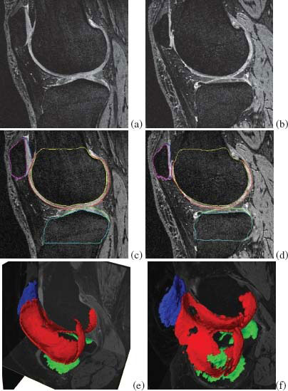
FIGURE 10.17
3D segmentation of knee cartilages. Images from a knee minimally affected by osteoarthritis shown on the left. Severe cartilage degeneration shown on the right. (a,b) Original images. (c,d) The same slice with bone/cartilage segmentation. (e,f) Cartilage segmentation shown in 3D, note the cartilage thinning and “holes” in panel (f). Reprinted, with IEEE permission, from [4].

¹ If desired, $δ_{i}^{l}$ and $δ_{i}^{u}$ may be defined to be location specific (i.e., $δ_{i}^{l}$ and $δ_{i}^{u}$ may vary from column to column).

..................Content has been hidden....................

You can't read the all page of ebook, please click here login for view all page.

Table of Contents for 10 Optimal Simultaneous Multisurface and Multiobject Image Segmentation

Create new playlist

Sign In

Sign Up

Table of Contents for
10 Optimal Simultaneous Multisurface and Multiobject Image Segmentation