5 Targeted Image Segmentation Using Graph Methods

Traditional image segmentation is the process of subdividing an image into smaller regions based on some notion of homogeneity or cohesiveness among groups of pixels. Several prominent traditional segmentation algorithms have been based on graph theoretic methods [1, 2, 3, 4, 5, 6]. However, these methods have been notoriously difficult to quantitatively evaluate since there is no formal definition of the segmentation problem (see [7, 8] for some approaches to evaluating traditional segmentation algorithms).

In contrast to the traditional image segmentation scenario, many real-world applications of image segmentation instead focus on identifying those pixels belonging to a specific object or objects (which we will call targeted segmentation) for which there are some known characteristics. In this chapter, we focus only on the extraction of a single object (i.e., labeling each pixel as object or background). The segmentation of a specific object from the background is not just a special case of the traditional image segmentation problem that is restricted to two labels. Instead, a targeted image segmentation algorithm must input the additional information that determines which object is being segmented. This additional information, which we will call target specification, can take many forms: user interaction, appearance models, pairwise pixel affinity models, contrast polarity, shape models, topology specification, relational information, and/or feature inclusion. The ideal targeted image segmentation algorithm could input any or all of the target specification information that is available about the target object and use it to produce a high-quality segmentation.

Graph-theoretic methods have provided a strong basis for approaching the targeted image segmentation problem. One aspect of graph-theoretic methods that has made them so appropriate for this problem is that it is fairly straightforward to incorporate different kinds of target specification (or, at least, to prove that they are NP-hard). In this chapter, we begin by showing how the image graph may be constructed to accommodate general target specification and review several of the most prominent models for targeted image segmentation, with an emphasis on their commonalities. Having established the general models, we show specifically how the various types of target specification may be used to identify the target object.

A targeted image segmentation algorithm consists of two parts: a target specification that identifies the desired object and a regularization that completes the segmentation from the target specification. The goal of the regularization algorithm is to incorporate as little or as much target specification that is available and still produce a meaningful segmentation of the target object under generic assumptions of object cohesion. We first treat different methods of performing the regularization in a general framework before discussing how targeting information can be combined with the regularization. In our opinion, the regularization is the core piece of a targeted segmentation algorithm and defines the primary difference between different algorithms. The target specification informs the algorithm what is known about the target object, while the regularization determines the segmentation with an underlying model of objects that describes what is unknown about the object. Put differently, the various varieties of target specification may be combined fairly easily with different types of regularization methods, but it is the regularization component that determines how the final output segmentation will be defined from that information.

The exposition will generally be in terms of nodes and edges rather than pixels or voxels. Although nodes are typically identified with pixels or voxels, we do not want to limit our exposition to 2D or 3D (unless otherwise specified), and we additionally want to allow for graphs representing images derived from superpixels or more general structures (see Chapter 1).

Before beginning, we note that targeted image segmentation is very similar to the alpha-matting problem in Chapter 9, and many of the methods strongly overlap. The main difference between targeted image segmentation and alpha-matting is that alpha-matting necessarily produces a real-valued blending coefficient at each pixel, while targeted segmentation ultimately seeks to identify which pixels belong to the object (although real-valued confidences can be quite useful in targeted segmentation problems). Moreover, the literature on alpha-matting and targeted segmentation is typically focused on different aspects of the problem. Alpha-matting algorithms are usually interactive with the assumption that most pixels are labeled except those at the boundary (a trimap input). The focus for alpha-matting algorithms is therefore on getting a meaningful blending coefficient for pixels that contain some translucency such as hair or fur. In contrast, the focus in targeted segmentation algorithms is on both interactive or automatic solutions in which there are few or no prelabeled pixels. Targeted image segmentation methods using graphs are also closely related to semisupervised clustering algorithms. The primary differences between targeted image segmentation and semi-supervised clustering are: (1) The graph in image segmentation is typically a lattice rather than an arbitrary network, (2) The pixels in image segmentation are embedded in RN $ℝ^{N}$ , while a semi-supervised clustering may not have an embedding, and (3) Pixels are associated with values (e.g., RGB) while points to be clustered may not be. The effect of these differences is that some ways of providing target specification in image segmentation may not apply to semi-supervised clustering, such as shape, appearance models, genus, or object features.

5.1 The Regularization of Targeted Image Segmentation

Many algorithms have been proposed for regularizing the targeted image segmentation problem. One class of algorithms were formulated originally in a continuous domain and optimized using active contours or level sets. More recently, a second set of algorithms have been formulated directly on a graph (or reformulated on a graph from the original continuous definition) and optimized using various methods in combinatorial and convex optimization. Algorithms in both classes ultimately take the form of finding a minimum of the energy

E(x) = Eunary(x) + λEbinary(x), $E (x) = E_{unary} (x) + λ E_{binary} (x),$

(5.1)

in which xi ∈ R $x_{i} \in ℝ$ , 0 ≤ x_i ≤ 1; any pixels known to belong to the object (foreground) set, υi ∈ F $υ_{i} \in ℱ$ , would be assigned x_i = 1, and any pixels known to belong to the background set, υi ∈ B $υ_{i} \in B$ , would be assigned x_i = 0. The parameter λ may be used to control the relative weighting of the two terms (i.e., to modulate the confidence of the information represented by each term). Any pixels with known labels are termed seeds or sometimes scribbles (since they are often provided interactively). The value of x at a pixel therefore represents the affinity of that pixel to belong to object (and may also be interpreted as the success probability of a Bernoulli distribution modeling the pixel label [9]). Given an x that minimizes (5.1), a hard segmentation may be produced by assigning a pixel with value x_i > θ = 0.5 to the object and a pixel with value x_i ≤ θ to the background. Since the explicit goal of a targeted segmentation algorithm is to find a hard (binary) segmentation, it may seem strange that the above formulation performs the optimization over a real-valued x and sets a threshold, since it is well known that relaxing a general binary optimization problem to real values and thresholding can produce a suboptimal solution to the binary optimization problem [10]. However, as we will see shortly, several targeted segmentation algorithms which are not derived from optimization problems may be computed by performing the above optimization over real values and then thresholding at 0.5. Consequently, for these algorithms, there is no “relaxation” since the algorithms are not defined by optimization problems except insofar as the computations to perform the algorithms may be viewed as a continuous-valued optimization. Furthermore, it has been shown that those segmentation algorithms reviewed below that are defined as binary optimization problems still produce minimal binary solutions, whether they are optimized over binary variables or whether the solution is produced by thresholding a real-valued solution.

The first term in (5.1) is called the unary term since it is formulated as a function of each node independently. Similarly, the binary term is formulated as a function of both nodes and edges. The unary term is sometimes called the data or region term and the binary term is sometimes called the boundary term. In this work we will prefer the terms unary and binary to describe these terms, since we will see that the unary and binary terms are used to represent many types of target specification beyond just data and boundaries.

All of the regularization methods discussed in this section are formulated on a primal graph in which each pixel is associated with a node to be labeled. This formulation has the longest history in the image segmentation literature, and it is now best understood how to perform target specification with different information for regularization algorithms with this formulation. Furthermore, primal methods are easy to apply in 3D since we can simply associate each voxel with a node. Recently, various authors have been looking into formulations of regularization and target specification on the dual graph (starting with [11, 12] and then extended by [13, 14, 15, 16]), but this thread is too recent to further review here. See [17, 12] for more information on primal and dual graphs in this context.

5.1.1 Power Watershed Formalism

Five prominent algorithms for targeted image segmentation were shown to unite under a single form of the unary and binary terms that differ only by a parameter choice. Specifically, if we let the unary and binary terms equal (termed the basic energy model in [17])

Eunary(x) = ∑υi∈ VwqBi |xi− 0|p + wqFi |xi − 1|p, $E_{unary} (x) = \sum_{υ_{i} \in V} w_{B i}^{q} {| x_{i} - 0 |}^{p} + w_{F i}^{q} {| x_{i} - 1 |}^{p},$

(5.2)

and

Ebinary(x) = ∑eij∈ Ewqij |xi− xj|p, $E_{binary} (x) = \sum_{e_{i j} \in ℰ} w_{i j}^{q} {| x_{i} - x_{j} |}^{p},$

(5.3)

then Table 5.1 shows how different targeted segmentation algorithms are derived from differing values of p and q. The values and meaning of the unary object weight, wFi $w_{F i}$ , unary background weight, wBi $w_{B i}$ , and binary weights w_ij vary with respect to the target specification and are discussed more extensively in Section 5.2. Unless otherwise stated, we assume that wFi, wBi > 0, ∀υi ∈ V $w_{F i}, w_{B i} > 0, \forall υ_{i} \in V$ and w_ij > 0, ∀eij ∈ E $\forall e_{i j} \in ℰ$ . Specifically, it was shown in [18, 9, 19, 20] that the graph cuts algorithm [21, 22], the random walker algorithm [23], the shortest paths (geodesic) algorithm [24, 25], the conventional watershed algorithm [26] and the power watershed algorithm [27] could all be seen as providing a solution to the same energy (with different parameters), despite very different motivations and optimization methods. Specifically, the graph cuts algorithm optimizes the energy with a max-flow computation [28], the random walker algorithm optimizes the energy with a linear system solve, the shortest paths algorithm uses Dijkstra’s algorithm to perform the optimization (or [29]), and the two watershed algorithms use speciality algorithms devised for this optimization, which are detailed in [26, 27]. It is important to note that the random walker and shortest paths algorithms are not motivated by optimization problems, but rather by determining the likelihood that a random walker first reaches a seed or by determining which pixel is connected by shortest path to the seeds. In fact, it is quite surprising that the random walker and shortest path algorithms, with motivations not derived from optimization, can still be viewed as the thresholded solutions to an optimization problem. However, it is important not to confuse the fact that random walker and shortest paths are equivalent to thresholding continuous optimization problems with a relaxation of a binary optimization problem. In fact, it is surprising that the optimization problems representing each algorithm (regardless of formulation) are so directly related to each other with simple parameter changes.

The generalized shortest path algorithm may also be considered to further subsume additional algorithms. In particular, the image foresting transform [24] showed that algorithms based on fuzzy connectedness [30, 31] could also be viewed as special cases of the shortest path algorithm (albeit with a different notion of distance). Furthermore, the GrowCut algorithm [32], derived in terms of cellular automata, was also shown to be equivalent to the shortest path based algorithm [33]. Consequently, the GrowCut algorithm can be seen as directly belonging to the framework described in Table 5.1, while the fuzzy connectedness algorithms are closely related (it has been suggested in [34] that fuzzy connectedness segmentation is obtained by a binary optimization of the case for p → ∞ and q → ∞). A recent treatment of the connection between these algorithms, fuzzy connectedness and a few other algorithms may be found in Miranda and Falcão [35].

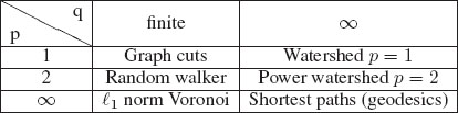
TABLE 5.1
Minimization of the general model presented in Equation (5.1) with Equations (5.2) and (5.3) leads to several well-known algorithms in the literature. This connection is particularly surprising since the random walker and shortest path algorithms were not originally formulated or motivated in the context of an energy optimization. Furthermore, graph cuts is often viewed as a binary optimization algorithm, even though optimization of Equation (5.1) for a real-valued variable leads to a cut of equal length (after thresholding the real-valued solution). Note that “∞” is used to indicate the solution obtained as the parameter approaches infinity (see [27] for details). The expression ℓ₁ norm Voronoi” is intended to represent an intuitive understanding of this segmentation on a 4-connected (2D) or 6-connected (3D) lattice.

The optimization of fractional values of p was considered in [36, 9], in which this algorithm was termed P-brush and optimized using iterative reweighted least squares. Additionally, it was shown in [36, 9] that the optimal solutions are strongly continuous as p varies smoothly. Consequently, a choice of q finite and p = 1.5 would yield an algorithm which was a hybrid of graph cuts and random walker. It was shown in [18, 36, 9] that if q is finite, lower values of p create solutions with increased shrinking bias, while higher values of p create solutions with increased sensitivity to the locations of user-defined seeds. Furthermore, it was shown that the metrication artifacts are removed for p = 2 (due to the connection with the Laplace equation [9]), but are present for the p = 1 and p = ∞ solutions.

The regularization algorithms in the power watershed framework all assume that some object and background information is specified in the form of hard constraints or unary terms. In practice, it is possible that the object is specified using only object hard constraints or unary terms. In this case, it is possible to extend the models in the power watershed framework with a generic background term such as a balloon force [37, 38] or by using the isoperimetric algorithm [5, 39], as shown in [17]

5.1.2 Total Variation and Continuous Max-Flow

One concern about the p = 1 and finite q model above (graph cuts) is the metrication issues that can arise as a result of the segmentation boundary being measured by the edges cut, which creates a dependence on the edge structure of the image lattice [9]. This problem has been addressed in the literature [40, 41] by adding more edges, but this approach can sometimes create computational problems (such as memory usage), particularly in 3D image segmentation. Consequently, the total variation and continuous max-flow algorithms are sometimes preferred over graph cuts because they (approximately) preserve the geometrical description of the solution as minimizing boundary length (surface area), but also reduce metrication errors (without additional memory) by using a formulation at the nodes in order to preserve rotational invariance [42, 43, 44, 20].

The total variation (TV) functional is most often expressed using a continuous domain (first used in computer vision by [45, 46]). However, formulations on a graph have been considered [47, 48]. Although TV was initially considered for image denoising, it is natural to apply the same algorithm to targeted segmentation by using an appropriate unary term and interpretation of the variable [44, 17]. In the formalism given in (5.1), the segmentation algorithm by total variation has the same unary term as (5.2), but the binary term is given by [48]

ETVbinary(x) = ∑υi ∈ V⎛⎝∑j, ∀eij ∈ Ewij |xi − xj|2⎞⎠p2. $E_{binary}^{TV} (x) = {\sum_{υ_{i} \in V} ({\sum_{j, \forall e_{i j} \in ℰ} w_{i j} | x_{i} - x_{j} |}^{2})}^{\frac{p}{2}} .$

(5.4)

However, note that some authors have preferred a node weighting for TV, which would instead give

ETVbinary(x) = ∑υi ∈ Vwi ⎛⎝∑j, ∀eij ∈ E|xi − xj|2⎞⎠p2. $E_{binary}^{TV} (x) = {\sum_{υ_{i} \in V} w_{i} ({\sum_{j, \forall e_{i j} \in ℰ} | x_{i} - x_{j} |}^{2})}^{\frac{p}{2}} .$

(5.5)

Since our discussions in Section 5.2 will treat node weights as belonging to the unary term and edge weights as belonging to the binary term, we will explicitly prefer the formulation given in Equation (5.4).

Optimization of the TV functional is generally more complicated than optimization of any of the algorithms in the power watershed framework. The TV functional is convex and may therefore be optimized with gradient descent [48], but this approach is typically too slow to be useful in many practical image segmentation situations. However, fast methods for performing TV optimization have appeared recently [49, 50, 51, 52], which makes these methods more competitive in speed compared to the algorithms in the power watershed framework described in Section 5.1.1.

The dual problem to minimizing the TV functional is often considered to be the continuous max-flow (CMF) problem [53, 54]. However, more recent studies have shown that this duality is fragile in the sense that weighted TV and weighted max-flow are not always dual in the continuous domain [55] and that standard discretizations of both TV and CMF are not strongly dual to each other (weighted or unweighted) [20]. Consequently, it seems best to consider the CMF problem to be a separate, but related, problem to TV. Although CMF was introduced into the image segmentation literature in its continuous form [42], subsequent work has shown how to write the CMF problem on an arbitrary graph [20]. This graph formulation of the continuous max-flow problem (termed combinatorial continuous max-flow) is not equivalent to the standard max-flow problem formulated on a graph by Ford and Fulkerson [56]. The difference between combinatorial continuous max-flow (CCMF) and conventional max-flow is that the capacity constraints for conventional max-flow are defined on edges, while the capacity constraints for CCMF are defined on nodes. As with TV, this formulation on nodes affords a certain rotational independence which leads to a reduction of metrication artifacts.

The native CMF and CCMF problems do not have explicit unary terms in the sense defined in Equation (5.1), although such terms could be added via the dual of these algorithms. The incorporation of unary terms into the CCMF model was addressed specifically in [20]. Furthermore, both the CMF and CCMF problems for image segmentation were formulated using node weights [42, 20] to represent unary terms as well as flow constraints (similar to the second TV represented in Equation (5.5)). However, as with the second TV, this use of node weights in both contexts does not fit the formalism adopted in Section 5.2. Although the standard formulations use node weights for the “binary” term (the capacity constraints), this could be easily modified to adopt edge weights in the manner formulated by [53] for the continuous formulation of CMF or adopted by [48] for the formulation of an edge-weighted TV. A fast optimization method for the CCMF problem was given by Couprie et al. in [20].

5.2 Target Specification

In the previous discussion we discussed the basic regularization models underlying a variety of targeted segmentation algorithms. However, before these regularization models can be applied for targeted object segmentation it is necessary to specify additional information. Specifically, the targeting information may be encoded on the graph by manipulating unary term weights, binary term weights, constraints, and/or extra terms to Equation (5.1). Therefore, some types of target specification will have little effect on our ability to find exact solutions for the algorithms in Section 5.1, while other kinds of target specification force us to employ approximate solutions only (e.g., the objective function becomes nonconvex).

In this section we will review a variety of ways to provide a target specification that have appeared in the literature. In general, multiple sources of target specification may be combined by simply including all constraints, or by adding together the weights defining the unary term and binary term specifications. However, note that some form of target specification is necessary to produce a nontrivial solution of the regularization algorithms in Section 5.1. While discussing different methods of target specification, we will deliberately be neutral to the choice of underlying regularization model that was presented in Section 5.1. The general form of all the models given in Equation (5.1) can accommodate any of the target specification methods that will be reviewed, since each model can utilize target information encoded in user interaction, additional terms, unary node weights, and/or binary edge weights.

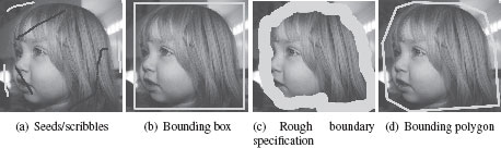
FIGURE 5.1
Different user interaction modes that have been used to specify the segmentation target. These interaction modes may also be populated automatically (e.g., by finding a bounding box automatically).

5.2.1 Segmentation Targeting With User Interaction

An easy way of specifying the target object is to allow a user to specify the desired object. By building a system that can incorporate user interaction, it becomes possible to distribute a system that is capable of segmenting a variety of (a priori unknown) targets rather than a single known target. Present-day image editing software (e.g., Adobe Photoshop) always includes some sort of interactive targeted image segmentation tool.

There are essentially three methods in the literature to allow a user to specify the target object. The first method is to label some pixels inside/outside the object, the second method is to specify some indication of the object boundary and the third is to specify the sub-region within the image that contains the object. Figure 5.2.1 gives an example of these methods of user interaction.

5.2.1.1 Seeds and Scribbles

In this user interaction mode, the user specifies labels (typically with a mouse or touchscreen) for some pixels inside the target object and for some pixels outside the object. These user-labeled pixels are often called seeds, scribbles, or hard constraints. Assume that all pixels labeled object (foreground) belong to the set F $F$ and all pixels labeled background belong to set B $B$ where F ∩ B = 0 $F \cap B = 0$ . These seeds are easily incorporated into (5.1) by performing the optimization subject to the constraints that x_i = 1 if υi ∈ F $υ_{i} \in F$ and x_i = 0 if υi ∈ B $υ_{i} \in B$ .

An equivalent way of writing these seeds is to cast them as unary terms, such that (in the context of (5.2)) wFi = ∞ $w_{F i} = \infty$ if υi ∈ F $υ_{i} \in F$ and wBi = ∞ $w_{B i} = \infty$ if υi ∈ B $υ_{i} \in B$ . In this way, the unary terms effectively enforce the hard constraints. Enforcement of the seeds through unary terms has two advantages. The first advantage is that the grid structure of the image lattice is not disrupted by adding a unary term, which can be important for the efficient implementation of some algorithms (see [57]). The second advantage is that the unary formulation of the seeds allows one to incorporate some level of uncertainty in the seed locations by setting the weights to some finite value instead of infinity. In this setting, a smaller weight encodes less confidence in the location while a larger weight encodes greater confidence. Note that it is possible to incorporate some seeds as hard constraints and others as unary terms. In this way, one may build a system that requires only object seeds (set as hard constraints) in which the background seeds were set at every other pixel (i.e., B = V − F $B = V - F$ ) via low-weight unary terms. Consequently, the user would only need to provide object interactions to specify the target, which would reduce the amount of user time necessary to achieve the segmentation.

Other interfaces for user seeding have also been explored in the literature. For example, Heiler et al. [58] suggested allowing the user to specify that two pixels belong to different labels without specifying which pixel is object and which is background. This sort of interaction may be incorporated by introducing a negative edge weight to encode repulsion [59]. Specifically, if υ_i and υ_j are specified to have an opposite label, this constraint can be encoded by introducing a new edge e_ij with weight w_ij = −∞, which forces the optimization in Equation (5.1) to place these nodes on opposite sides of the partition. Note, however, that the introduction of negative edge weights requires an explicit constraint on the optimization in Equation (5.1) to force 0 ≤ x_i ≤ 1 in order to avoid the possibility of an unbounded solution.

5.2.1.2 Object Boundary Specification

Another natural user interface is to roughly specify part or all of the desired object boundary. This boundary specification has been encoded into the above algorithms in one of two ways by editing a polygon or by providing a soft brush. Boundary specification is substantially different in 2D and 3D segmentation, since 2D object boundaries are contours and 3D object boundaries are surfaces. In general, approaches that have a used boundary specification have operated mainly in 2D image segmentation.

A similar boundary-based approach to interactively specify the object boundary was proposed by Wang et al. [60], who asks the user to freehand paint the boundary with a large brush (circle) such that the true boundary lies inside the painted region. Given this painted region (which the authors assumed could be painted quickly), hard constraints for the object label were placed on the inside of the user-painted boundary and hard constraints for the background label were placed on the outside of the user-painted boundary. See Chapter 9 for more details on this user interface.

5.2.1.3 Sub-Region Specification

Sub-region specification was introduced to save the user time, as an alternative to placing seeds or marking the object boundary (even roughly). The most common approach to sub-region specification has been to ask the user to draw a box surrounding the target object [61, 62, 63, 64]. This interface is convenient for a user, but also has the advantage that it is easy to connect to an automatic preprocessing algorithm to produce a fully automated segmentation, that is, by using machine learning with a sliding window to find the correct bounding box (a Viola-Jones type detector [65]). We showed with a user study in [64] that a single box input was sufficient to fully specify a target object over a wide variety of object sizes, shapes, backgrounds and homogeneity levels, even when the images do not contain explicit semantic content.

Rother et al. [61] introduced one of the most well-known methods for making use of the bounding box interface for segmentation called GrabCut. In the GrabCut algorithm background constraints are placed on the outside of the user-supplied box, while allowing an appearance model to drive the object segmentation in an iterative manner (see Section 5.2.2). Lempitsky et al. [62] suggested constraining the segmentation such that the user-drawn box is tightly fit to the resulting segmentation, which they term the tightness prior. Grady et al. [64] adopted the same interface for the PIBS algorithm (probabilistic isoperimetric box segmentation), which used no unary term, but instead set directed edge weights based on an estimate of the object appearance probability for each pixel and applied the isoperimetric segmentation algorithm [5, 39] with the bounding box set as background seeds.

5.2.2 Segmentation Targeting with Appearance Information

The purpose of an appearance model is to use statistics about the distribution of intensity/color/texture etc., inside, and outside the object to specify the target object. In most cases, appearance models are incorporated as unary terms in the segmentation. Broadly speaking, there are two approaches to appearance modeling. In the first approach, the model is established once prior to performing segmentation. In the second approach, the appearance model is learned adaptively from the segmentation to produce a joint estimation of both the appearance model and the image segmentation.

5.2.2.1 Prior Appearance Models

In the earliest appearance of these targeted segmentation models, it was assumed that the probability was known that would match the image intensity/color at each pixel to an object or background label. Specifically, if g_i represents the intensity/color at pixel υ_i, then it was assumed that p(g_i|x_i = 1) and p(g_i|x_i = 0) were known. The representation of p(g_i|x_i) may be parametric or nonparametric. Presumably, these probabilities are based on training data or known a priori (as in the classical case of binary image segmentation). Given known values of the probabilities, p(_{g_i}|x_i = 1) and p(g_i|x_i = 0), these probabilities are used to affect the unary terms in the above model by setting, for (5.2), wFi= p(gi|xi = 1) $w_{F i} = p (g_{i} | x_{i} = 1)$ and wBi = p(gi|xi = 0) $w_{B i} = p (g_{i} | x_{i} = 0)$ . Note that wFi = −log (p(gi|xi = 1)) $w_{F i} = - \log (p (g_{i} | x_{i} = 1))$ and wBi = −log (p(gi|xi = 0)) $w_{B i} = - \log (p (g_{i} | x_{i} = 0))$ have also been used instead in conjunction with a derivation from an markov random field (see [21]).

If the probability models are not known a priori, then they may be estimated from user-drawn seeds [22]. Specifically, the seeds may be viewed as a sample of the object and background distributions. Consequently, these samples may be used with a kernel estimation method to estimate p(g_i|x_i = 1) and p(g_i|x_i = 0). When g represents multichannel image data (e.g., color), then a parametric method, such as a Gaussian mixture model, is typically preferred [66].

In addition to modeling p(g_i|x_i) directly, several groups have used a transformed version of g_i to establish unary terms. The purpose of this transformation is to model objects with a more complex appearance, which may be better characterized by a texture than by a simple intensity/color distribution. Specifically, transformations which appear in the literature include the outputs of textons/filter banks [67], structure tensors [68, 69], tensor voting [70], or features learned on-the-fly from image patches [71]. Formally, we may view these methods as estimating p(gWi|xi) $p (g_{W_{i}} | x_{i})$ , where $W_{i}$ is a window of pixels centered on pixel υ_i.

Sometimes the target segmentation has a known shape that can be exploited to model $p (g_{W_{i}} | x_{i})$ by estimating the similarity of a window around pixel υ_i to the known shape. This matching may be viewed as the application of a shape filter to produce a response that is interpreted as $p (g_{W_{i}} | x_{i})$ . Shape filters of this nature have usually been applied to elongated or vessel-like objects. Vessel-like objects have frequently been detected using properties of the Hessian matrix associated with a window centered on a pixel. Frangi et al. [72] used the eigenvalues of the Hessian matrix to define a vesselness measure that was applied in Freiman et al. [73] as a unary term for defining the vesselness score. A similar approach was used by Esneault et al. [74] who used a cylinder matching function to estimate $p (g_{W_{i}} | x_{i})$ and gave a unary term for the segmentation of vessel-like objects. Using shape information in this way is fundamentally different from the shape models described in Section 5.2.4 since the use of shape information here is to directly estimate $p (g_{W_{i}} | x_{i})$ via a filter response, while the models in Section 5.2.4 use the fit of a top-down model to fit a unary term.

5.2.2.2 Optimized Appearance Models

Models in the previous section assumed that the appearance models were known a priori or could be inferred from a presentation of the image and/or user interaction. However, one may also view the appearance model as a variable, which may be inferred from the segmentation process. In this setting, we may rewrite Equation (5.1) as

$E (P, x) = E_{unary} (P, x) + λ E_{binary} (P, x),$

(5.6)

in which P represents the appearance model, that is, P is shorthand for $w_{F i}$ and $w_{B i}$ . Segmentation algorithms which take this form typically alternate between iterations in which (5.6) is optimized for x relative to a fixed P and then optimized for P relative to a fixed x. This alternation is a result of the difficulty in finding a joint global optimization for both P and x, and the fact that each iteration of the alternating optimization approach is guaranteed to produce a solution with lower or equal energy from the previous iteration.

The most classic approach with an optimized appearance model is the Mumford-Shah model [75, 76] in which $w_{F i}$ and $w_{B i}$ are a function of an idealized object and background image, a and b. Specifically, we may follow [77] to write the piecewise smooth Mumford-Shah model as

$\begin{array}{r} E (P, x) = & (x^{T} {(g - a)}^{2}) + {(1 - x)}^{T} {(g - b)}^{2})) + \\ μ (x^{T} {| A |}^{T} {(A a)}^{2} + {(1 - x)}^{T} {| A |}^{T} {(A b)}^{2}) + λ E_{binary} (x), \end{array}$

(5.7)

where A is the incidence matrix (see definition in Chapter 1). The μ and λ parameters are free parameters used to weight the relative importance of the terms. The form presented here represents a small generalization of the classic form, also in [77], in which x was assumed to be binary and $E_{binary} (x) = \sum_{e_{i j}} w_{i j} | x_{i} - x_{j} |$ , that is, that p = q = 1 in (5.3). The optimization of Equation (5.7) may be performed by alternating steps in which a, b are fixed and x is optimized with steps in which x is fixed an a, b are optimized. Since each alternating iteration of the optimization is convex, the energy of successive solutions will monotonically decrease.

A simplified version of the Mumford-Shah model is known as the piecewise constant model (also called the Chan-Vese model [78]) in which a and b are represented by constant functions (i.e., a_i = k₁, $\forall υ_{i} \in V$ and b_i = k₂, $\forall υ_{i} \in V$ ). We may write the piecewise constant Mumford-Shah model as

$E (P, x) = (x^{T} {(g - k_{1} 1)}^{2} + {(1 - x)}^{T} {(g - k_{2} 1)}^{2}) + λ E_{binary} (x) .$

(5.8)

Therefore, the piecewise constant Mumford-Shah model neglects the second term in (5.7). The same alternating optimization of Equation (5.8) is possible, except that the optimization for a and b is extremely simple, that is, $a_{i} = k_{1} = \frac{x^{T} g}{x^{T} 1}$ and $b_{i} = k_{2} = \frac{{(1 - x)}^{T} g}{{(1 - x)}^{T} 1}$ .

A similar optimized appearance model was presented in the GrabCut algorithm [61] which was applied to color images. In this approach, the object and background color distributions were modeled as two Gaussian mixture models (GMM) with unknown parameters. Specifically, GrabCut optimizes the model

$E (θ, x) = H (θ_{F}, g, x) + H (θ_{B}, g, (1 - x)) + λ E_{binary} (x),$

(5.9)

in which θ represents the parameters for the GMM and $H (θ_{F}, g_{i}, x_{i})$ represents the (negative log) probability that g_i belongs to the object GMM (see [61] for more details). As with the optimization of the Mumford-Shah models, the optimization of the GrabCut energy also proceeds by alternating between estimation of x (given a fixed $θ_{F}$ and $θ_{B}$ ) and estimation of $θ_{F}$ and $θ_{B}$ (given a fixed x).

5.2.3 Segmentation Targeting with Boundary Information

A widespread method for specifying a target is to impose a model of the target object boundary appearance that may be incorporated into the edge weights of the binary term in Equation (5.3). Depending on the form of the boundary regularization, the edge weights represent either the affinity between pixels (i.e., small weight indicates a disconnect between pixels) or the distance between pixels (i.e., large weight indicates a disconnect between pixels). These descriptions are reciprocal to each other, as described in [17], i.e., $w_{affinity} = \frac{1}{w_{distance}}$ . To simplify our discussion in this section, we assume that the edge weights represent affinity weights.

The most classical approach to incorporating boundary appearance into a targeted segmentation method is to assume that the object boundary is more likely to pass between pixels with large image contrast. The functions which are typically used to encode boundary contrast were originally developed in the context of non-convex descriptions of the image denoising problem [79, 80, 81] and later enshrined in the segmentation literature via the normalized cuts method [3] and the geodesic active contour method [82]. Since these weighting functions may be derived from corresponding M-estimators [83, 17] we use the term Welsch function to describe

$w_{i j} = \exp (- β {‖ g_{i} - g_{j} ‖}_{2}^{2}),$

(5.10)

and Cauchy function to describe

$w_{i j} = \frac{1}{1 + β {‖ g_{i} - g_{j} ‖}_{2}^{2}},$

(5.11)

where g_i represents the intensity (grayscale) value or a color (or multispectral) vector associated with pixel υ_i. In practice, these edge weighting functions are often slightly altered to avoid zero weights (which can disconnect the graph) and to accommodate the dynamic range in different images. To avoid zero edge weights, a small constant may be added (e.g., ϵ = 1e⁻⁶). The dynamic range of an image may be accommodated by dividing β by a constant ρ where $ρ = \max_{e_{i j}} {‖ g_{i} = g_{j} ‖}_{2}^{2}$ or $ρ = {mean}_{e_{i j}} {‖ g_{i} - g_{j} ‖}_{2}^{2}$ . Another possibility for choosing ρ more robustly is to choose the edge difference corresponding to the 90th percentile of all edge weights (as done in [80]). In one study comparing the effectiveness of the Welsch and Cauchy functions, it was determined that the Cauchy function performed slightly better on average (and is also computationally less expensive to compute at runtime) [84].

One problem with the assumption that the object boundary passes between pixels with large image contrast is that the difference between the target object and its boundary may be more subtle than some contrasts present in the image. For example, soft tissue boundaries in a medical computed tomography image are often much lower contrast than the tissue/air boundaries present at the lung or external body interfaces. Another problem is that the contrast model is only appropriate for objects with a smooth appearance, but is less appropriate for textured objects. To account for low contrast or textured objects, the weighting functions in (5.10) and (5.11) may be modified by replacing g_i with H(g_i) where H is a function which maps raw pixel content to a transform space where the object appearance is relatively constant. For example, if the target object exhibits a striped texture, then H could represent the response of a “stripe filter” which causes the target object to produce a relatively uniform response. In fact, any of the appearance models described in Section 5.2.2 can be used to establish more sophisticated boundary models by adopting H(g_i) = p(g_i|x_i = 1). This sort of model can be very effective even when the target object has a relatively smooth appearance, since it can be used to detect boundaries which are more subtle in the original image [84, 64].

5.2.3.1 Boundary Polarity

A problem with the boundary models in the previous section is that they describe the probability that the boundary passes between two pixels without accounting for the direction of the transition [85]. This problem is illustrated in Figure 5.2 which shows how a more subtle correct boundary may be overwhelmed by a strong boundary with the wrong transition. Alternately, we may say that the target specification may be ambiguous without a specification of the boundary polarity, as illustrated in Figure 5.2.

A model of the target object appearance allows us to specify that the target segmentation boundary transitions from the pixels which have the object appearance to pixels which do not [86]. Mechanically, this polarity model has been specified by formulating the graph models on a directed graph in which each undirected edge e_ij is replaced by two directed edges e_ij and e_ji such that w_ij and w_ji may or may not be equal [85, 86]. Given an appearance model from Section 5.2.2, it was proposed in [86] to formulate these directed edges via

$w_{i j} = {\begin{array}{l} \exp (- β_{1} {‖ H (g_{i}) - H (g_{j}) ‖}_{2}^{2}) & if H (g_{i}) > H (g_{j}), \\ \exp (- β_{2} {‖ H (g_{i}) - H (g_{j}) ‖}_{2}^{2}) & else, \end{array}$

(5.12)

where β₁ > β₂. In other words, boundary transitions from pixels matching the target object appearance to pixels that do not are less costly (from the standpoint of energy minimization). Note that the same approach could be applied using the Cauchy weighting formula.

Edge weights have been shown to play the role on a graph that corresponds to the metric in conventional multivariate calculus [17]. In this respect, it was shown that the weights of a directed graph could be viewed specifically as representing a Finsler metric on a graph [87].

5.2.4 Segmentation Targeting with Shape Information

Object shape is a natural and semantic descriptor for specifying a target segmentation. However, even semantically, the description of object shape can take many forms, from general descriptions (e.g., “The object is elongated”) to parametric descriptions (e.g., “The object is elliptical” or “The object looks like a leaf”) and feature-driven descriptions (e.g., “The object has four long elongated parts and one short elongated part connected to a broad base”). Targeted segmentation algorithms using shape information have followed the same patterns of description. In this section we will cover both implicit (general) shape descriptions and explicit (parametric) shape descriptions. The discussion on feature-driven object descriptions will be postponed to Section 5.2.5.

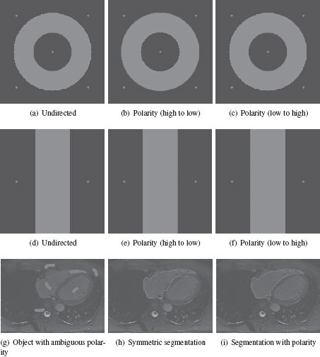
FIGURE 5.2
(a-f) Ambiguous synthetic images where the use of polarity can be used to appropriately specify the target object. (g-i) A real image with ambiguous boundary polarity. It is unclear whether the endocardium (inside) or epicardium (outside) is desired. Using an undirected model chooses the endocardium (inside) in one part of the segmentation and the epicardium (outside) in the other part. However, polarity information can be used to specify the target as the endocardium (inside boundary).

It is important to distinguish between those shape models in which the graph is being used to regularize the appearance of a shape feature and those models in which the regularization provides the shape model. To illustrate this point, consider the segmentation of elongated shapes. The shape can be encoded by either a standard regularization of an elongation appearance measure (e.g., a vesselness measure from Section 5.2.2.1 with TV or random walker regularization) or by a regularization that biases the segmentation toward elongated solutions (e.g., a curvature regularization) or both. Put differently, we must distinguish between a data/unary term that measures elongation and a binary or higher order term that promotes elongation. Section 5.2.2.1 treated the appearance-based type, and this section treats the regularization type.

5.2.4.1 Implicit Shape Models

The targeted segmentation models described in Section 5.1 implicitly favor large, compact (blob-like) shapes. Specifically, for an object of fixed area with a single central seed, the targeted algorithms described in Section 5.1 favor a circle (up to metrication artifacts) when applied on a graph with weights derived from Euclidean distance of the edge length. This property may be seen in graph cuts and TV because a circle is the shape that minimizes the boundary length over all shapes with a fixed area (known classically from the isoperimetric problem). The shortest path algorithm also finds a circle because the segmentation returns all pixels within a fixed distance from the central seed (where the distance is fixed by the area constraint). Similarly, the random walker algorithm also favors a circle, since the segmentation includes all pixels within a fixed resistance distance (where the distance is fixed by the area constraint).

Although many target segmentation objects are compact in shape, it is not always the case. For an example in medical imaging, thin blood vessels are a common segmentation target, as are thin surfaces such as the grey matter in cerebral cortex. Segmenting these objects can be accomplished with the algorithms in Section 5.2 if the bias toward compact shapes can be overcome by a strong appearance term or a sharp boundary contrast (leading to an unambiguous binary term via the edge weighting). However, in many real images we cannot rely on strong appearance terms or boundary contrast. A variety of graph-based models have been introduced recently that measure a discrete notion of the curvature of a segmentation boundary [88, 89, 90, 14, 91]. Specifically, these models seek to optimize a discrete form of the elastica equation proposed by Mumford [92], which he showed to embody the Bayes optimal solution of a model of curve continuity. The continuous form of the elastica equation is

$\begin{matrix} e (C) = \int_{C} (a + b κ^{2}) d s & a, b > 0, \end{matrix}$

(5.13)

where κ denotes scalar curvature, and ds is the arc length element. At the time of writing, there are several different ideas that have been published for writing an appropriate discretization of this model and performing the optimization. Since it is not yet clear if these or some other idea will become preferred for performing curvature optimization, we leave the details of the various methods to the references.

Another implicit shape model in the literature biases the segmentation toward rectilinear shapes [93]. Specifically, this model takes advantage of the work by Zunic and Rosin [94] on rectilinear shape measurement, where it was shown that the class of shapes which minimize the ratio

$Q (P) = \frac{{Per}_{1} (P)}{{Per}_{2} (P)},$

(5.14)

are rectilinear shapes (with respect to the specified X and Y axis). Here, Per₁(P) denotes the ℓ₁ perimeter of shape P according to the specified X and Y axis. Similarly, Per₂(P) denotes the perimeter of shape P with the ℓ₂ metric. In other words,

${Per}_{1} (P) = \int | u^{'} (t) | + | υ^{'} (t) | d t,$

(5.15)

${Per}_{2} (P) = \int \sqrt{{u^{'}}^{2} (t) + {υ^{'}}^{2} (t)} d t,$

(5.16)

for some parametrization u(t), υ(t) of the shape boundary P. Note that (5.14) does not provide a rotationally invariant measure of rectilinearity (i.e., this approach assumes that the rectangular object roughly aligns with the image axes). Noting that the perimeter of the segmentation may be measured by an ℓ₁ or ℓ₂ metric, depending on the edge structure and weighting (see [93, 40]), it is possible to create two graphs to represent the ℓ₁ and ℓ₂ metrics, displayed in Figure 5.2.4.1. Since a rectilinear shape is small in ℓ₁ compared to ℓ₂, this method of implicit rectilinear shape segmentation was called the opposing metrics method. Given an ℓ₁ graph, represented by Laplacian matrix L₁ and an ℓ₂ graph, represented by Laplacian matrix L₂, a binary indicator vector x that minimizes the ratio

$E_{rect} (x) = \frac{{Per}_{1} (Ω x)}{{Per}_{2} (Ω x)} \approx \frac{x^{T} L_{1} x}{x^{T} L_{2} x},$

(5.17)

will be a rectilinear shape. Consequently, the term in (5.17) may be used as a regularization to implicitly bias the segmentation toward a rectilinear shape. Note that the authors of [93] chose to relax the binary constraint on x to produce a generalized eigenvector problem, which may be solved efficiently for sparse matrices using established methods. A final observation of the energy in (5.17) is that the numerator fits precisely into the power watershed framework in Section 5.1, particularly (5.3). Consequently, one interpretation of the opposing metrics method of [93] is that it relies on the same sort of binary regularization as before, except that it uses a second graph (represented by the denominator) to modify the implicit default shape from a circle to a rectilinear shape.

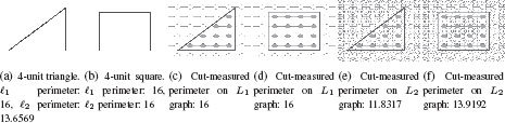
FIGURE 5.3
A rectilinear shape is known to minimize the ratio of the perimeter measured with an ℓ₁ metric and the perimeter measured with an ℓ₂ metric [94]. It is possible to measure the perimeter of a object, expressed as a cut, with respect to various metrics with arbitrary accuracy by adjusting the graph topology and weighting [40]. The opposing metrics strategy for segmenting rectilinear shapes is to look for the segmentation that minimizes the cut with respect to one graph, L₁, while maximizing the cut with respect to a second graph, L₂.

In this section it was shown how most traditional first-order graph-based segmentation algorithms implicitly bias the segmentation toward compact circular shapes. However, by modifying the functionals to include the higher-order term of curvature, it was possible to remove the bias toward compact shapes, meaning that the energy was better suited for elongated objects such as blood vessels. Additionally, by further modifying the functional to include a second graph (present in the denominator) it is possible to implicitly bias the segmentation toward rectilinear objects. One advantage of these implicit methods is that it has been frequently demonstrated that a global optimum of the energy functional is possible to achieve, meaning that the algorithms have no dependence on initialization. In the next section we consider those methods that add an explicit shape bias by using training data or a parameterized shape. While this approach allows for the targeting of more complex shapes, a global optimum becomes very hard to achieve, meaning that these methods rely on a good initialization.

5.2.4.2 Explicit Shape Models

One of the first approaches to incorporating an explicit shape model into graph-based segmentation was by Slabaugh and Unal [95] who constrained the segmentation to return an elliptical object. The idea was effectively to add a third term to the conventional energy,

$E (x, θ) = E_{data} (x) + E_{binary} (x) + E_{ellipse} (x, θ),$

(5.18)

where θ represents the parameters of an ellipse, and

$E_{ellipse} (x, θ) = \sum_{υ_{i} \in V} | M_{i}^{θ} - x_{i} |,$

(5.19)

where M^θ represents the mask corresponding to the ellipse parameterized by θ such that pixels inside the ellipse are marked ‘1’ and pixels outside the mask are marked ‘0’.

Since finding a global optimum of (5.18) is challenging, Slabaugh and Unal [95] performed an alternating optimization of (5.18) in which x was first optimized for with a fixed θ (in [95] this optimization was performed only over a narrow band surrounding the current solution) and then θ was optimized for a fixed x. Although this formulation was introduced for an elliptical shape, it is clear that it could be extended to any parameterized shape.

A problem with the above approach to targeting with an explicit shape model is that complex shapes may be difficult to effectively parameterize and fit to a fixed solution for x. Consequently, an alternative approach is to use a shape template that can be fit to the current segmentation. This was the approach adopted by Freedman and Zhang [96], who used a distance function computed on the fit template to modify the edge weights to promote a segmentation matching the template shape.

Freedman and Zhang’s method for incorporating shape information suffers from the fact that it does not account for any shape variability, but rather assumes that the target segmentation for a particular image closely matches the template. Shape variability of a template may be accounted for using a PCA decomposition of a set of training shapes, as described in the classical work of Tsai et al. [97] using a level set framework. A similar method of accounting for shape variability was formulated on a graph by Zhu-Jacquot and Zabih [98] who model the shape template, U, as

$U = \bar{U} + \sum_{k = 1}^{K} w_{k} U^{k},$

(5.20)

where U is the mean shape and U^k is the kth principal component of a set of training shapes. The weights w_k and the set of rigid transformations is optimized at each iteration of [98] with the current segmentation x fixed. Then, the segmentation x is determined using the fit shape template to define a unary term (as opposed to the binary term in [96]).

5.2.5 Segmentation Targeting with Object Feature Information

In some segmentation tasks, substantial training data is available to provide sufficient target specification to specify the desired object. Typically, we assume that the training data contains both images and segmentations of the desired object. From this training data, it may be possible to learn a set of characteristic geometric or appearance features to describe the target object and relationships between those features.

One of the first methods to adopt this approach in the context of targeted graph-based segmentation was the ObjCut method of Kumar et al. [99]. In this algorithm, the authors build on the work of pictorial structures [100] and assume that the target object may be subdivided into a series of parts that may vary in relationship to each other. The composition of the model into parts (and their relationships) is directed by the algorithm designer, but the appearance and variation of each part model is learned using the training data. The algorithm operates by fitting the orientation and scale parameters of the parts and then using the fitted pictorial structure model to define unary terms for the segmentation. Levin and Weiss build on this work to employ a conditional random field to perform joint training of the model using both the high-level module and the low-level image data [101].

5.2.6 Segmentation Targeting with Topology Information

If the target object has a known topology, then it is possible to use this information to find an appropriate segmentation. Unfortunately, specification of a global property of the segmentation, like topology, has been challenging. Topology specification has seen increasing interest recently, however, all of the work we are aware of has focused on this sort of specification in the context of the graph cuts segmentation algorithm, in which the problems have generally been shown to be NP-Hard. Two types of topology specification have been explored in the literature—Connectivity and genus.

5.2.6.1 Connectivity Specification

When the segmentation target is a single object, it is reasonable to assume that the object is connected (although this assumption is not always correct, as in the case of occlusion). A segmentation, $S$ , is considered connected if $\forall υ_{i} \in S$ , $υ_{j} \in S$ , ∃ π_ij, s.t. if υ_k ∈ π_ij, then $υ_{k} \in S$ .

In general, any of the segmentation methods in Section 5.1 do not guarantee that the returned segmentation is connected. However, under certain conditions, it is known that any algorithm in the power watershed framework will guarantee connectivity. The conditions for guaranteed connectivity are: (1) No unary terms, (2) The set of object seeds is a connected set, and (3) For all edges, w_ij > 0. Given these conditions, any algorithm in the power watershed framework produces a connected object, since the x value for every nonseeded node is always between the x values of its neighbors, meaning that if x_i is above the 0.5 threshold (i.e., included in the segmentation $S$ ), then it has at least one neighboring node that is also above threshold (i.e., included in the segmentation $S$ ). More specifically, any solution x that minimizes

$E (x) = {\sum_{e_{i j} \in E} w_{i j}^{q} | x_{i} - x_{j} |}^{p},$

(5.21)

for some choice of p ≥ 0 and q ≥ 0 has the property for any nonseeded node that

$x_{i} = \arg \min \sum_{j} w_{i j}^{q} {| x_{i} - x_{j} |}^{p},$

(5.22)

for established values of all x_j. There is some maximum x_max and minimum x_min among the neighbors of υ_i. Specifically, we know that x_min ≤ x_i ≤ x_max since any x_i lower than x_min would give a larger value in the argument of (5.22) than x_min. The same argument applies to x_max, meaning that the optimal x_i falls within the range of its neighbors, and consequently there exists a neighbor υ_j for which x_j ≥ x_i. Since $S$ is defined as the set of all nodes for which x_i > 0.5, then any node in $S$ contains at least one neighbor in $S$ , meaning that there is a connected path from any node in $S$ to a object seed. By assumption, the set of object seeds is connected, so every node inside $S$ is connected to every other node inside $S$ . Since this principle applies to any choice of p and q, then under the above conditions the object is guaranteed to be connected for graph cuts, random walker, shortest paths, watershed, power watershed, and fuzzy connectedness. A slight modification of the same argument also allows us to guarantee that TVSeg produces a connected object segmentation under very similar conditions.

In practice, the conditions that guarantee connectedness of the segmentation may be violated in those circumstances in which unary terms are used or where the set of input seeds is not connected. In these situations, it has been proven for graph cuts that the problem of finding the minimal solution while guaranteeing connectivity is NP-Hard [102]. To our knowledge, it is still unknown whether it is possible to guarantee connectivity for any of the other algorithms in the power watershed framework. Vincente et al. chose to approximate a related, but simpler, problem [103]. Specifically, Vincente et al. consider that two points in the image have been designated for connectivity (either interactively or automatically) and provide an algorithm that generates a segmentation that approximately optimizes the graph cut criterion while guaranteeing the connectivity of the designated points. Vincente et al. then demonstrate that their algorithm will sometimes find the global optimum, while guaranteeing connectivity of the designated points, on real-world images. Nowozin and Lampert adopted a different approach to the problem of enforcing connectivity for the graph cuts algorithm by instead solving a related optimization problem for the global optimum [104].

5.2.6.2 Genus Specification

Many target objects have a known genus, particularly in biomedical imaging. This genus information can help the algorithm avoid leaving internal voids (if the object is known to be simply connected) or falsely filling voids when the object is known to have internal holes. There has been little work to date on genus specification for targeted graph-based segmentation algorithms. The first work on this topic is by Zeng et al. [102] who proved that it is NP-hard to optimize the graph cuts criterion with a genus constraint (the other algorithms in the power watershed framework have not been examined with a genus constraint). However, Zeng et al. provide an algorithm that enforces a genus constraint (keeping the genus of an initial segmentation) while approximately optimizing the graph cuts criterion. Their algorithm is based on the topology-preserving level sets work of [105] which uses the simple point concept from digital topology [106]. Effectively, if an algorithm adds or subtracts only simple points from an initial segmentation, then the modified segmentation will have the same genus as the original. Zeng et al. show that their algorithm for genus preservation has the same asymptotic complexity as the graph cuts algorithm without genus constraints. The algorithm by Zeng et al. for genus specification was further simplified and improved by Danek and Maska [107]. Therefore, these genus specification algorithms can be used to enforce object connectivity by making the initial input segmentation connected.

5.2.7 Segmentation Targeting by Relational Information

Our focus in this chapter is on the specification of target information to define the segmentation of a single object. However, certain kinds of target specification can only be defined for an object in relation to other objects. In this section, we examine this relational target specification and so slightly expand our scope beyond singleobject segmentation.

Similar to Chapter 10, the goal of using relational information (sometimes known as geometric constraints) is to enforce a certain geometrical relationship between two objects. Specifically, the following relationships between two regions ( $A$ and $B$ ) were studied by Delong and Boykov [108]:

1. Containment: Region $B$ must be inside region $A$ , perhaps with a repulsion force between boundaries.

2. Exclusion: Regions $A$ and $B$ cannot overlap at any pixel, perhaps with a repulsion force between boundaries.

3. Attraction: Penalize the area $A - B$ , exterior to $B$ , by some cost α > 0 per unit area. Thus, $A$ will prefer not to grow too far beyond the boundary of $B$ .

The basic idea of [108] is to create two graphs, $G^{A} = {V^{A}, ℰ^{A}}$ and $G^{B} = {V^{B}, ℰ^{B}}$ , each to represent the segmentation of $A$ or $B$ . The segmentation of $A$ on $G^{A}$ is represented by the indicator vectors $x^{A}$ (and $x^{B}$ , respectively, for $G^{B}$ ). Then, a new energy term is introduced

$E_{Geometric} (x^{A}, x^{B}) = \sum_{υ_{i} \in V^{A}, υ_{j} \in V^{B}} w_{i j} (x_{i}, x_{j}),$

(5.23)

meaning that the two graphs $G^{A}$ and $G^{B}$ are effectively fully connected with each other. The weights to encode the three geometric relationships are given in 5.2.7. Delong and Boykov studied the optimization of (5.23) in the context of the graph cuts model and found that containment and attraction are easy to optimize since the energy is submodular. However, the energy for the exclusion relationship is non-submodular and therefore more challenging except under limited circumstances (see [108] for more details). Furthermore, encoding these geometrical relationships for more than two objects can lead to optimization problems for which a global optimum is not easy to obtain. Ulén et al. [109] applied this model to cardiac segmentation and further expanded the discussion of encoding these constraints for multiple objects. These geometric interactions have not been studied in the context of any of the other regularization models of Section 5.1, but they would be straightforward to incorporate.

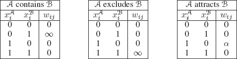
TABLE 5.2
Three types of relational information between two objects.

5.3 Conclusion

Traditional image segmentation seeks to subdivide an image into a series of meaningful objects. In contrast, a targeted segmentation algorithm uses input target specification to determine a specific desired object. A targeted image segmentation algorithm consists of two parts: a target specification which specifies the desired object and a regularization that completes the segmentation from the target specification. The ideal regularization algorithm could incorporate as little or as much target specification that was available and still produce a meaningful segmentation of the target object.

Targeted image segmentation algorithms have matured in recent years. Today, there are many effective regularization methods available with efficient optimization algorithms. Additionally, many different types of target specification have been accommodated, including prior information about appearance, boundary, shape, user interaction, learned features, relational information, and topology.

Despite this increasing maturity, more remains to be done. The regularization methods reviewed in Section 5.1 are not as effective for segmenting elongated or sheet-like objects. Additionally, the use of prior information about higher-order statistics of the target object have just started to be explored (see Chapter 3 for more on this topic). Finally, the exploration has been piecemeal of the optimization of different types of target specification combined with different regularization methods (or combined with other types of target specification). The optimization of different regularization methods in the presence of different types of target specification has not always been treated in the literature. We believe that the future will see the development of new and exciting methods for regularization that may be optimized efficiently in the presence of one or more different types of target specification, which will bring the community to the point of effectively solving the targeted image segmentation problem.

Bibliography

[1] C. Zahn, “Graph theoretical methods for detecting and describing Gestalt clusters,” IEEE Transactions on Computation, vol. 20, pp. 68–86, 1971.

[2] Z. Wu and R. Leahy, “An optimal graph theoretic approach to data clustering: Theory and its application to image segmentation,” IEEE Transactions on Pattern Analysis and Machine Intelligence, vol. 15, no. 11, pp. 1101–1113, 1993.

[3] J. Shi and J. Malik, “Normalized cuts and image segmentation,” IEEE Transactions on Pattern Analysis and Machine Intelligence, vol. 22, no. 8, pp. 888–905, Aug. 2000.

[4] P. F. Felzenszwalb and D. P. Huttenlocher, “Efficient graph-based image segmentation,” International Journal of Computer Vision, vol. 59, no. 2, pp. 167–181, September 2004.

[5] L. Grady and E. L. Schwartz, “Isoperimetric graph partitioning for image segmentation,” IEEE Transactions on Pattern Analysis and Machine Intelligence, vol. 28, no. 3, pp. 469–475, March 2006.

[6] J. Roerdink and A. Meijster, “The watershed transform: definitions, algorithms, and parallellization strategies,” Fund. Informaticae, vol. 41, pp. 187–228, 2000.

[7] Y. Zhang, “A survey on evaluation methods for image segmentation,” Pattern Recognition, vol. 29, no. 8, pp. 1335–1346, 1996.

[8] D. Martin, C. Fowlkes, D. Tal, and J. Malik, “A database of human segmented natural images and its application to evaluating segmentation algorithms and measuring ecological statistics,” in Proc. ICCV, 2001.

[9] D. Singaraju, L. Grady, A. K. Sinop, and R. Vidal, “P-brush: A continuous valued MRF for image segmentation,” in Advances in Markov Random Fields for Vision and Image Processing, A. Blake, P. Kohli, and C. Rother, Eds. MIT Press, 2010.

[10] G. L. Nemhauser and L. A. Wolsey, Integer and Combinatorial Optimization. Wiley-Interscience, 1999.

[11] L. Grady, “Computing exact discrete minimal surfaces: Extending and solving the shortest path problem in 3D with application to segmentation,” in Proc. of CVPR, vol. 1, June 2006, pp. 69–78.

[12] ——, “Minimal surfaces extend shortest path segmentation methods to 3D,” IEEE Trans. on Pattern Analysis and Machine Intelligence, vol. 32, no. 2, pp. 321–334, Feb. 2010.

[13] T. Schoenemann, F. Kahl, and D. Cremers, “Curvature regularity for region-based image segmentation and inpainting: A linear programming relaxation,” in Proc. of CVPR. IEEE, 2009, pp. 17–23.

[14] P. Strandmark and F. Kahl, “Curvature regularization for curves and surfaces in a global optimization framework,” in Proc. of EMMCVPR, 2011, pp. 205–218.

[15] F. Nicolls and P. Torr, “Discrete minimum ratio curves and surfaces,” in Proc. of CVPR. IEEE, 2010, pp. 2133–2140.

[16] T. Windheuser, U. Schlickewei, F. Schmidt, and D. Cremers, “Geometrically consistent elastic matching of 3D shapes: A linear programming solution,” in Proc. of ICCV, vol. 2, 2011.

[17] L. Grady and J. R. Polimeni, Discrete Calculus: Applied Analysis on Graphs for Computational Science. Springer, 2010.

[18] A. K. Sinop and L. Grady, “A seeded image segmentation framework unifying graph cuts and random walker which yields a new algorithm,” in Proc. of ICCV 2007, IEEE Computer Society. IEEE, Oct. 2007.

[19] C. Allène, J.-Y. Audibert, M. Couprie, and R. Keriven, “Some links between extremum spanning forests, watersheds and min-cuts,” Image and Vision Computing, vol. 28, no. 10, 2010.

[20] C. Couprie, L. Grady, L. Najman, and H. Talbot, “Combinatorial continuous max flow,” SIAM J. on Imaging Sciences, vol. 4, no. 3, pp. 905–930, 2011.

[21] D. Greig, B. Porteous, and A. Seheult, “Exact maximum a posteriori estimation for binary images,” Journal of the Royal Statistical Society, Series B, vol. 51, no. 2, pp. 271–279, 1989.

[22] Y. Boykov and M.-P. Jolly, “Interactive graph cuts for optimal boundary & region segmentation of objects in N-D images,” in Proc. of ICCV 2001, 2001, pp. 105–112.

[23] L. Grady, “Random walks for image segmentation,” IEEE Trans. on Pattern Analysis and Machine Intelligence, vol. 28, no. 11, pp. 1768–1783, Nov. 2006.

[24] A. X. Falcão, R. A. Lotufo, and G. Araujo, “The image foresting transformation,” IEEE Transactions on Pattern Analysis and Machine Intelligence, vol. 26, no. 1, pp. 19–29, 2004.

[25] X. Bai and G. Sapiro, “A geodesic framework for fast interactive image and video segmentation and matting,” in ICCV, 2007.

[26] S. Beucher and F. Meyer, “The morphological approach to segmentation: the watershed transformation,” in Mathematical Morphology in Image Processing, E. R. Dougherty, Ed. Taylor & Francis, Inc., 1993, pp. 433–481.

[27] C. Couprie, L. Grady, L. Najman, and H. Talbot, “Power watershed: A unifying graph-based optimization framework,” IEEE Trans. on Pat. Anal. and Mach. Int., vol. 33, no. 7, pp. 1384–1399, July 2011.

[28] Y. Boykov and V. Kolmogorov, “An experimental comparison of min-cut/max-flow algorithms for energy minimization in vision,” IEEE Transactions on Pattern Analysis and Machine Intelligence, pp. 1124–1137, 2004.

[29] L. Yatziv, A. Bartesaghi, and G. Sapiro, “A fast O(N) implementation of the fast marching algorithm,” Journal of Computational Physics, vol. 212, pp. 393–399, 2006.

[30] J. Udupa and S. Samarasekera, “Fuzzy connectedness and object definition: Theory, algorithms, and applications in image segmentation,” Graphical Models and Image Processing, vol. 58, pp. 246–261, 1996.

[31] P. Saha and J. Udupa, “Relative fuzzy connectedness among multiple objects: Theory, algorithms, and applications in image segmentation,” Computer Vision and Image Understanding, vol. 82, pp. 42–56, 2001.

[32] V. V. and K. V., “GrowCut — Interactive Multi-Label N-D Image Segmentation,” in Proc. of Graphicon, 2005, pp. 150–156.

[33] A. Hamamci, G. Unal, N. Kucuk, and K. Engin, “Cellular automata segmentation of brain tumors on post contrast MR images,” in Proc. of MICCAI. Springer, 2010, pp. 137–146.

[34] K. C. Ciesielski and J. K. Udupa, “Region-based segmentation: Fuzzy connectedness, graph cut and related algorithms,” in Biomedical Image Processing, ser. Biological and Medical Physics, Biomedical Engineering, T. M. Deserno, Ed. Springer-Verlag, 2011, pp. 251–278.

[35] P. A. V. Miranda and A. X. Falcão, “Elucidating the relations among seeded image segmentation methods and their possible extensions,” in Proceedings of Sibgrapi, 2011.

[36] L. G. Dheeraj Singaraju and R. Vidal, “P-brush: Continuous valued MRFs with normed pairwise distributions for image segmentation,” in Proc. of CVPR 2009, IEEE Computer Society. IEEE, June 2009.

[37] L. D. Cohen, “On active contour models and balloons,” CVGIP: Image understanding, vol. 53, no. 2, pp. 211–218, 1991.

[38] L. Cohen and I. Cohen, “Finite-element methods for active contour models and balloons for 2-D and 3-D images,” IEEE Transactions on Pattern Analysis and Machine Intelligence, vol. 15, no. 11, pp. 1131–1147, 1993.

[39] L. Grady and E. L. Schwartz, “Isoperimetric partitioning: A new algorithm for graph partitioning,” SIAM Journal on Scientific Computing, vol. 27, no. 6, pp. 1844–1866, June 2006.

[40] Y. Boykov and V. Kolmogorov, “Computing geodesics and minimal surfaces via graph cuts,” in Proceedings of International Conference on Computer Vision, vol. 1, October 2003.

[41] O. Danˇek and P. Matula, “An improved Riemannian metric approximation for graph cuts,” Discrete Geometry for Computer Imagery, pp. 71–82, 2011.

[42] B. Appleton and H. Talbot, “Globally optimal surfaces by continuous maximal flows,” IEEE Transactions on Pattern Analysis and Machine Intelligence, vol. 28, no. 1, pp. 106–118, Jan. 2006.

[43] M. Unger, T. Pock, and H. Bischof, “Interactive globally optimal image segmentation,” Inst. for Computer Graphics and Vision, Graz University of Technology, Tech. Rep. 08/02, 2008.

[44] M. Unger, T. Pock, W. Trobin, D. Cremers, and H. Bischof, “TVSeg - Interactive total variation based image segmentation,” in Proc. of British Machine Vision Conference, 2008.

[45] D. Shulman and J.-Y. Herve, “Regularization of discontinuous flow fields,” in Proc. of Visual Motion, 1989, pp. 81–86.

[46] L. Rudin, S. Osher, and E. Fatemi, “Nonlinear total variation based noise removal algorithms,” Physica D, vol. 60, no. 1-4, pp. 259–268, 1992.

[47] S. Osher and J. Shen, “Digitized PDE method for data restoration,” in In Analytical-Computational methods in Applied Mathematics, E. G. A. Anastassiou, Ed. Chapman & Hall/CRC,, 2000, pp. 751–771.

[48] A. Elmoataz, O. Lézoray, and S. Bougleux, “Nonlocal discrete regularization on weighted graphs: A framework for image and manifold processing,” IEEE Transactions on Image Processing, vol. 17, no. 7, pp. 1047–1060, 2008.

[49] A. Chambolle, “An algorithm for total variation minimization and applications,” J. Math. Imaging Vis., vol. 20, no. 1–2, pp. 89–97, 2004.

[50] J. Darbon and M. Sigelle, “Image restoration with discrete constrained total variation part I: Fast and exact optimization,” Journal of Mathematical Imaging and Vision, vol. 26, no. 3, pp. 261–276, Dec. 2006.

[51] X. Bresson, S. Esedoglu, P. Vandergheynst, J.-P. Thiran, and S. Osher, “Fast global minimization of the active contour/snake model,” Journal of Mathematical Imaging and Vision, vol. 28, no. 2, pp. 151–167, 2007.

[52] A. Chambolle and T. Pock, “A first-order primal-dual algorithm for convex problems with applications to imaging,” Journal of Mathematical Imaging and Vision, vol. 40, no. 1, pp. 120–145, 2011.

[53] M. Iri, “Theory of flows in continua as approximation to flows in networks,” Survey of Mathematical Programming, 1979.

[54] G. Strang, “Maximum flows through a domain,” Mathematical Programming, vol. 26, pp. 123–143, 1983.

[55] R. Nozawa, “Examples of max-flow and min-cut problems with duality gaps in continuous networks,” Mathematical Programming, vol. 63, no. 2, pp. 213–234, Jan. 1994.

[56] L. R. Ford and D. R. Fulkerson, “Maximal flow through a network,” Canadian Journal of Mathematics, vol. 8, pp. 399–404, 1956.

[57] L. Grady, “A lattice-preserving multigrid method for solving the inhomogeneous poisson equations used in image analysis,” in Proc. of ECCV, ser. LNCS, D. Forsyth, P. Torr, and A. Zisserman, Eds., vol. 5303. Springer, 2008, pp. 252–264.

[58] M. Heiler, J. Keuchel, and C. Schnörr, “Semidefinite clustering for image segmentation with a-priori knowledge,” in Proc. of DAGM, 2005, pp. 309–317.

[59] S. X. Yu and J. Shi, “Understanding popout through repulsion,” in Proc. of CVPR, vol. 2. IEEE Computer Society, 2001.

[60] J. Wang, M. Agrawala, and M. Cohen, “Soft scissors: An interactive tool for realtime high quality matting,” in Proc. of SIGGRAPH, 2007.

[61] C. Rother, V. Kolmogorov, and A. Blake, ““GrabCut” — Interactive foreground extraction using iterated graph cuts,” in ACM Transactions on Graphics, Proceedings of ACM SIGGRAPH 2004, vol. 23, no. 3. ACM, 2004, pp. 309–314.

[62] V. Lempitsky, P. Kohli, C. Rother, and T. Sharp, “Image segmentation with a bounding box prior,” in Proc. of ICCV, 2009, pp. 277–284.

[63] H. il Koo and N. I. Cho, “Rectification of figures and photos in document images using bounding box interface,” in Proc. of CVPR, 2010, pp. 3121–3128.

[64] L. Grady, M.-P. Jolly, and A. Seitz, “Segmentation from a box,” in Proc. of ICCV, 2011.

[65] P. Viola and M. Jones, “Robust real-time face detection,” International Journal of Computer Vision, vol. 57, no. 2, pp. 137–154, 2004.

[66] A. Blake, C. Rother, M. Brown, P. Perez,, and P. Torr, “Interactive image segmentation using an adaptive GMMRF model,” in Proc. of ECCV, 2004.

[67] X. Huang, Z. Qian, R. Huang, and D. Metaxas, “Deformable-model based textured object segmentation,” in Proc. of EMMCVPR, 2005, pp. 119–135.

[68] J. Malcolm, Y. Rathi, and A. Tannenbaum, “A graph cut approach to image segmentation in tensor space,” in Proc. Workshop Component Analysis Methods, 2007, pp. 18–25.

[69] S. Han, W. Tao, D. Wang, X.-C. Tai, and X. Wu, “Image segmentation based on grabcut framework integrating multiscale nonlinear structure tensor,” IEEE Trans. on TIP, vol. 18, no. 10, pp. 2289–2302, Oct. 2009.

[70] H. Koo and N. Cho, “Graph cuts using a Riemannian metric induced by tensor voting,” in Proc. of ICCV, 2009, pp. 514–520.

[71] J. Santner, M. Unger, T. Pock, C. Leistner, A. Saffari, and H. Bischof, “Interactive texture segmentation using random forests and total variation,” in Proc. of BVMC, 2009.

[72] A. F. Frangi, W. J. Niessen, K. L. Vincken, and M. A. Viergever, “Multiscale vessel enhancement filtering,” in Proc. of MICCAI, ser. LNCS, 1998, pp. 130–137.

[73] M. Freiman, L. Joskowicz, and J. Sosna, “A variational method for vessels segmentation: Algorithm and application to liver vessels visualization,” in Proc. of SPIE, vol. 7261, 2009.

[74] S. Esneault, C. Lafon, and J.-L. Dillenseger, “Liver vessels segmentation using a hybrid geometrical moments/graph cuts method,” IEEE Trans. on Bio. Eng., vol. 57, no. 2, pp. 276–283, Feb. 2010.

[75] D. Mumford and J. Shah, “Optimal approximations by piecewise smooth functions and associated variational problems,” Comm. Pure and Appl. Math., vol. 42, pp. 577–685, 1989.

[76] A. Tsai, A. Yezzi, and A. Willsky, “Curve evolution implementation of the Mumford-Shah functional for image segmentation, denoising, interpolation, and magnification,” IEEE Transactions on Image Processing, vol. 10, no. 8, pp. 1169–1186, 2001.

[77] L. Grady and C. Alvino, “The piecewise smooth Mumford-Shah functional on an arbitrary graph,” IEEE Transactions on Image Processing, vol. 18, no. 11, pp. 2547–2561, Nov. 2009.

[78] T. Chan and L. Vese, “Active contours without edges,” IEEE Transactions on Image Processing, vol. 10, no. 2, pp. 266–277, 2001.

[79] S. Geman and D. McClure, “Statistical methods for tomographic image reconstruction,” in Proc. 46th Sess. Int. Stat. Inst. Bulletin ISI, vol. 52, no. 4, Sept. 1987, pp. 4–21.

[80] P. Perona and J. Malik, “Scale-space and edge detection using anisotropic diffusion,” IEEE Transactions on Pattern Analysis and Machine Intelligence, vol. 12, no. 7, pp. 629–639, July 1990.

[81] D. Geman and G. Reynolds, “Constrained restoration and the discovery of discontinuities,” IEEE Transactions on Pattern Analysis and Machine Intelligence, vol. 14, no. 3, pp. 367–383, March 1992.

[82] V. Caselles, R. Kimmel, and G. Sapiro, “Geodesic active contours,” International journal of computer vision, vol. 22, no. 1, pp. 61–79, 1997.

[83] M. J. Black, G. Sapiro, D. H. Marimont, and D. Heeger, “Robust anisotropic diffusion,” IEEE Transactions on Image Processing, vol. 7, no. 3, pp. 421–432, March 1998.

[84] L. Grady and M.-P. Jolly, “Weights and topology: A study of the effects of graph construction on 3D image segmentation,” in Proc. of MICCAI 2008, ser. LNCS, D. M. et al., Ed., vol. Part I, no. 5241. Springer-Verlag, 2008, pp. 153–161.

[85] Y. Boykov and G. Funka-Lea, “Graph cuts and efficient N-D image segmentation,” International Journal of Computer Vision, vol. 70, no. 2, pp. 109–131, 2006.

[86] D. Singaraju, L. Grady, and R. Vidal, “Interactive image segmentation of quadratic energies on directed graphs,” in Proc. of CVPR 2008, IEEE Computer Society. IEEE, June 2008.

[87] V. Kolmogorov and Y. Boykov, “What metrics can be approximated by geo-cuts, or global optimization of length/area and flux,” in Proc. of the International Conference on Computer Vision (ICCV), vol. 1, 2005, pp. 564–571.

[88] T. Schoenemann, F. Kahl, and D. Cremers, “Curvature regularity for region-based image segmentation and inpainting: A linear programming relaxation,” in Proc. of ICCV, Kyoto, Japan, 2009.

[89] N. El-Zehiry and L. Grady, “Fast global optimization of curvature,” in Proc. of CVPR 2010, June 2010.

[90] ——, “Contrast driven elastica for image segmentation,” in Submitted to CVPR 2012, 2012.

[91] B. Goldluecke and D. Cremers, “Introducing total curvature for image processing,” in Proc. of ICCV, 2011.

[92] D. Mumford, “Elastica and computer vision,” Algebriac Geometry and Its Applications, pp. 491–506, 1994.

[93] A. K. Sinop and L. Grady, “Uninitialized, globally optimal, graph-based rectilinear shape segementation — The opposing metrics method,” in Proc. of ICCV 2007, IEEE Computer Society. IEEE, Oct. 2007.

[94] J. Zunic and P. Rosin, “Rectilinearity measurements for polygons,” IEEE Trans. on Pat. Anal. and Mach. Int., vol. 25, no. 9, pp. 1193–1200, Sept. 2003.

[95] G. Slabaugh and G. Unal, “Graph cuts segmentation using an elliptical shape prior,” in Proc. of ICIP, vol. 2, 2005.

[96] D. Freedman and T. Zhang, “Interactive graph cut based segmentation with shape priors,” in Proc. of CVPR, 2005, pp. 755–762.

[97] A. Tsai, A. Yezzi, W. Wells, C. Tempany, D. Tucker, A. Fan, W. E. Grimson, and A. Willsky, “A shape-based approach to the segmentation of medical images using level sets,” IEEE TMI, vol. 22, no. 2, pp. 137–154, 2003.

[98] J. Zhu-Jacquot and R. Zabih, “Graph cuts segmentation with statistical shape priors for medical images,” in Proc. of SITIBS, 2007.

[99] M. Kumar, P. H. S. Torr, and A. Zisserman, “Obj cut,” in Proc. of CVPR, vol. 1. IEEE, 2005, pp. 18–25.

[100] P. Felzenszwalb and D. Huttenlocher, “Efficient matching of pictorial structures,” in Proc. of CVPR, vol. 2. IEEE, 2000, pp. 66–73.

[101] A. Levin and Y. Weiss, “Learning to combine bottom-up and top-down segmentation,” in Proc. of ECCV. Springer, 2006, pp. 581–594.

[102] Y. Zeng, D. Samaras, W. Chen, and Q. Peng, “Topology cuts: A novel min-cut/max-flow algorithm for topology preserving segmentation in ND images,” Computer vision and image understanding, vol. 112, no. 1, pp. 81–90, 2008.

[103] S. Vicente, V. Kolmogorov, and C. Rother, “Graph cut based image segmentation with connectivity priors,” in Proc. of CVPR, 2008.

[104] S. Nowozin and C. Lampert, “Global interactions in random field models: A potential function ensuring connectedness,” SIAM Journal on Imaging Sciences, vol. 3, p. 1048, 2010.

[105] X. Han, C. Xu, and J. Prince, “A topology preserving level set method for geometric deformable models,” IEEE Transactions on Pattern Analysis and Machine Intelligence, pp. 755–768, 2003.

[106] G. Bertrand, “Simple points, topological numbers and geodesic neighborhoods in cubic grids,” Pattern Recognition letters, vol. 15, no. 10, pp. 1003–1011, 1994.

[107] O. Danek and M. Maska, “A simple topology preserving max-flow algorithm for graph cut based image segmentation,” in Proc. of the Sixth Doctoral Workshop on Mathematical and Engineering Methods in Computer Science, 2010, pp. 19–25.

[108] A. Delong and Y. Boykov, “Globally optimal segmentation of multi-region objects,” in Proc. of ICCV. IEEE, 2009, pp. 285–292.

[109] J. Uln, P. Strandmark, and F. Kahl, “Optimization for multi-region segmentation of cardiac MRI,” in Proc. of the MICCAI Workshop on Statistical Atlases and Computational Models of the Heart: Imaging and Modelling Challenges, 2011.

..................Content has been hidden....................

You can't read the all page of ebook, please click here login for view all page.

Table of Contents for 5 Targeted Image Segmentation Using Graph Methods

Create new playlist

Sign In

Sign Up

Table of Contents for
5 Targeted Image Segmentation Using Graph Methods