17

Tree-Walk Kernels for Computer Vision

Zaid Harchaoui

LEAR project-team
INRIA and LJK
655, avenue de l’Europe
38330 Montbonnot Saint-Martin, FRANCE

Email: [email protected]

Francis Bach

SIERRA project-team
INRIA and LIENS
23, avenue d’Italie
75214 Paris Cedex 13, FRANCE

Email: [email protected]

CONTENTS

17.1  Introduction

17.1.1  Related Work

17.2  Tree-Walk Kernels as Graph Kernels

17.2.1  Paths, Walks, Subtrees and Tree-Walks

17.2.2  Graph Kernels

17.3  The Region Adjacency Graph Kernel as a Tree-Walk Kernel

17.3.1  Morphological Region Adjacency Graphs

17.3.2  Tree-Walk Kernels on Region Adjacency Graphs

17.4  The Point Cloud Kernel as a Tree-Walk Kernel

17.4.1  Local Kernels

17.4.2  Positive Matrices and Probabilistic Graphical Models

17.4.3  Dynamic Programming Recursions

17.5  Experimental Results

17.5.1  Application to Object Categorization

17.5.2  Application to Character Recognition

17.5.3  Experimental Setting

17.6  Conlusion

17.7  Acknowledgments

Bibliography

17.1  Introduction

Kernel-based methods have proved highly effective in many applications because of their wide generality. As soon as a similarity measure leading to a symmetric positive-definite kernel can be designed, a wide range of learning algorithms working on Euclidean dot-products of the examples can be used, such as support vector machines [1]. Replacing the euclidian dot products by the kernel evaluations then corresponds to applying the learning algorithm on dot products of feature maps of the examples into a higher-dimensional space. Kernel-based methods are now well-established tools for computer vision—see, e.g. [2], for a review.

A recent line of research consists of designing kernels for structured data, to address problems arising in bioinformatics [3] or text processing. Structured data are data that can be represented through a labelled discrete structure, such as strings, labelled trees, or labelled graphs [4]. They provide an elegant way of including known a priori information, by using directly the natural topological structure of objects. Using a priori knowledge through kernels on structured data can be beneficial. It usually allows one to reduce the number of training examples to reach a high-performance accuracy. It is also an elegant way to leverage existing data representations that are already well developed by experts of those domains. Last but not least, as soon as a new kernel on structured data is defined, one can bring to bear the rapidly developing kernel machinery, and in particular semi-supervised learning—see, e.g., [5]—and kernel learning—see, e.g., [6].

We propose a general framework to build positive-definite kernels between images, allowing us to leverage, e.g., shape and appearance information to build meaningful similarity measures between images. On the one hand, we introduce positive-definite kernels between appearances as coded in region adjacency graphs, with applications to classification of images of object categories, as by [7, 8]. On the other hand, we introduce positive-definite kernels between shapes as coded in point clouds, with applications to classification of line drawings, as in [9, 10, 11]. Both types of information are difficult to encode into vector features without loss of information. For instance, in the case of shapes defined through point clouds, local and global invariances with respect to rotation/translation need to be encoded in the feature space representation.

A leading principle for designing kernels between structured objects is to decompose each object into parts and to compare all parts of one object to all parts of another object [1]. Even if there is an exponential number of such decompositions, which is a common case, this is numerically possible under two conditions: (a) the object must lead itself to an efficient enumeration of subparts, and (b) the similarity function between subparts (i.e., the local kernel), beyond being a positive-definite kernel, must be simple enough so that the sum over a potentially exponential number of terms can be recursively performed in polynomial time through factorization.

One of the most striking instantiations of this design principle are the string kernels [1], which consider all substrings of a given string but still allow efficient computation in polynomial time. The same principle can also be applied to graphs: intuitively, the graph kernels [12, 13] consider all possible subgraphs and compare and count matching subgraphs. However, the set of subgraphs (or even the set of paths) has exponential size and cannot be efficiently described recursively. By choosing appropriate substructures, such as walks or tree-walks, and fully factorized local kernels, matrix inversion formulations [14] and efficient dynamic programming recursion allow one to sum over an exponential number of substructures in polynomial time. We first review previous work on graph kernels. Then we present our general framework for tree-walk kernels in Section 17.2. In Section 17.3, we show how one can instantiate tree-walk kernels to build a powerful positive-definite similarity measure between region adjacency graphs. Then, in Section 17.4, we show how to instantiate tree-walk kernels to build an efficient positive-definite similarity measure between point clouds. Finally, in Section 17.5, we present experimental results of our tree-walk kernels respectively on object categorization, natural image classification, and handwritten digit classification tasks. This chapter is based on two conference papers [15, 16].

17.1.1  Related Work

The underlying idea of our tree-walk kernels is to provide an expressive relaxation of graph-matching similarity scores that yet yields a positive-definite kernel. The idea of matching graphs for the purpose of image classification has a long history in computer vision, and has been investigated by many authors [17, 18, 19]. However, the general graph matching problem is especially hard as most of the simple operations that are simple on strings (such as matching and edit distances) are NP-hard for general undirected graphs. Namely, while exact graph matching is unrealistic in our context, inexact graph matching is NP-hard and subgraph matching is NP-complete [4]. Hence, most work so far has focused on finding ingenious approximate solutions to this challenging problem [20]. An interesting line of research consists of overcoming graph matching problems by projecting graphs on strings by the so-called seriation procedure [18], and then using string edit distance [21] as a proxy to graph edit distance.

Designing kernels for image classification is also an active research topic. Since the work of [22], who investigated image classification with kernels on color histograms, many kernels for image classification were proposed. The bag-of-pixels kernels proposed in [23, 24] compare the color distributions of two images by using kernels between probability measures, and was extended to hierarchical multi-scale settings in [24, 25]; see [8] for an in-depth review.

Graph data occur in many application domains, and kernels for attributed graphs have received increased interest in the applied machine learning literature, in particular in bioinformatics [14, 13] and computer vision. Note that in this work, we only consider kernels between graphs (each data point is a graph), as opposed to settings where kernels are used to build a neighborhood graph from all the data points of a dataset [1].

Current graph kernels can roughly be divided in two classes: the first class is composed of non-positivedefinite similarity measures based on existing techniques from the graph matching literature, that can be made positive-definite by ad hoc matrix transformations; this includes the edit-distance kernel [26] and the optimal assignment kernel [27, 28]. In [26], the authors propose to use the edit distance between two graphs and directly plug it into a kernel to define a similarity measure between graphs. Kernels between shock graphs for pedestrian detection were also proposed in [29], allowing them to capture the topological structure of images. Our method efficiently circumvents the graph matching problem by soft-matching tree-walks, i.e., virtual substructures of graphs, in order to obtain kernels computable in polynomial time. Our kernels keep the underlying topological structure of graphs by describing them through tree-walks, while in graph seriation the topological structure somehow fades away by only retaining one particular substring of the graph. Moreover our kernels encompasses local information, by using segment histograms as local features, as well as global information, by summing up all soft matchings of tree-walks.

Another class of graph kernels relies on a set of substructures of the graphs. The most natural ones are paths, subtrees, and more generally subgraphs; however, they do not lead to positive-definite kernels with polynomial time computation algorithms—see, in particular, NP-hardness results by [12]—and recent work has focused on larger sets of substructures. In particular, random walk kernels consider all possible walks and sum a local kernel over all possible walks of the graphs (with all possible lengths). With a proper length-dependent factor, the computation can be achieved by solving a large sparse linear system [14, 30], whose running time complexity has been recently reduced [31]. When considering fixed-length walks, efficient dynamic programming recursions allow to drive down the computation time, at the cost of considering a smaller feature space. This is the approach we chose to follow here. Indeed, such an approach allows extensions to other types of substructures, namely “tree-walks”, whose abstract definition were first proposed by [12], that we now present. Several works later extended our approach to other settings, such as [32] for feature extraction from images and [33] for scene interpretation.

17.2  Tree-Walk Kernels as Graph Kernels

We first describe in this section the general framework in which we define tree-walk kernels. We shall then instantiate the tree-walk kernels respectively on region adjacency graphs in Section 17.3 and on point clouds in Section 17.4.

Let us consider two labelled undirected graphs g = (Vg, ϵg)g = (Vg, ϵg)$g=\left({\mathcal{V}}_g,{\mathit{ϵ}}_g\right)$ and $\mathscr{H}=\left({\mathcal{V}}_{\mathscr{H}},{\mathit{ϵ}}_{\mathscr{H}}\right)$, where ${\mathcal{V}}_g$ and ${\mathcal{V}}_{\mathscr{H}}$ denote the set of vertices resp. of g and $\mathscr{H},{\mathit{ϵ}}_g$ and $\mathscr{H}$ denote the set of edges resp. of g and $\mathscr{H}$. For the sake of clarity, we shall assume in the remainder that the vertex sets have the same cardinality; yet our framework can also handle vertex sets with different cardinality. Here, both the vertices and the edges can be labelled. Two types of labels are considered: attributes, which are denoted $a\left(\upsilon \right)\in {\mathcal{A}}_g$ for vertex $\upsilon \in {\mathcal{V}}_g$, and $b\left({\upsilon }^{\prime }\right)\in {\mathcal{A}}_{\mathscr{H}}$ for vertex ${\upsilon }^{\prime }\in {\mathcal{V}}_{\mathscr{H}}$ and positions, which are denoted $x\left(\upsilon \right)\in {\mathcal{X}}_g$ and $g\left({\upsilon }^{\prime }\right)\in {\mathcal{X}}_{\mathscr{H}}$. We make the distinction here between attributes and positions, since different kernels should be used to mesure similarity between attributes (respectively positions).

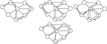
FIGURE 17.1
From left to right: path (red), 1-walk that is not a 2-walk (green), 2-walk that is not a 3-walk (blue), 4-walk (magenta).

17.2.1  Paths, Walks, Subtrees and Tree-Walks

Given an undirected graph g with vertex set $\mathcal{V}$, a path is a sequence of distinct connected vertices, while a walk is a sequence of possibly nondistinct connected vertices. In order to prevent the walks from going back and forth too quickly, we further restrain the set of walks. Such phenomenon was termed tottering by [34]). For any positive integer β, we define β-walks as walks such that any β + 1 successive vertices are distinct (1-walks are regular walks); see examples in Figure 17.1. Note that when the graph g is a tree (no cycles), then the set of 2-walks is equal to the set of paths. More generally, for any graph, β-walks of length β + 1 are exactly paths of length β + 1. Note that the integer β corresponds to the “memory” of the walk, i.e., the number of past vertices it needs to “remember” before going on.

A subtree of g is a subgraph of g with no cycles [4]. A subtree of g can thus be seen as a connected subset of distinct nodes of G with an underlying tree structure. The notion of walk is extending the notion of path by allowing vertices to be equal. Similarly, we can extend the notion of subtrees to tree-walks, where equal vertices can occur. More precisely, we define an α-ary tree-walk of depth γ of g as a rooted labelled α-ary tree of depth γ whose vertices share the same labels as the labels of the corresponding vertices in g. In addition, the labels of neighbors in the tree-walk must be neighbors in g (we refer to all allowed such set of labels as consistent labels). We assume that the tree-walks are not necessarily complete trees; i.e., each node may have less than α children. Tree-walks can be plotted on top of the original graph, as shown in Figure 17.5, and may be represented by a tree structure T over the vertex set {1,…, |T|} and a tuple of consistent but possibly nondistinct labels I ∈ V^|T| (i.e., the labels of neighboring vertices in T must be neighboring vertices in g). Finally, we only consider rooted subtrees, i.e., subtrees where a specific node is identified as the root. Moreover, all the trees that we consider are unordered trees (i.e., no order is considered among siblings). Yet, it is worthwhile to note that taking into account the order becomes more important when considering subtrees of region adjacency graphs.

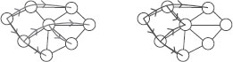
FIGURE 17.2
(Left) binary 2-tree-walk, which is in fact a subtree, (right) binary 1-tree-walk that is not a 2-tree-walk.

We can also define β-tree-walks, as tree-walks such that for each node in T, its label (which is an element of the original vertex set V) and the ones of all its descendants up to the β-th generation are all distinct. With that definition, 1-tree-walks are regular tree-walks (see Figure 17.2), and if α =1, we get back β-walks. From now on, we refer to the descendants up to the β-th generation as the β-descendants.

We let ${\mathcal{T}}_{\alpha ,\gamma }$ denote the set of rooted tree structures of depth less than γ and with at most α children per node; for example, ${\mathcal{T}}_{1,\gamma }$ is exactly the set of chain graphs of length less than γ. For $T\in {\mathcal{T}}_{\alpha ,\gamma }$, we denote ${\mathcal{J}}_{\beta }\left(T,G\right)$ the set of consistent labellings of T by vertices in V leading to β-tree-walks. With these definitions, a β-tree-walk of G is characterized by (a) a tree structure $T\in {\mathcal{T}}_{\alpha ,\gamma }$ and (b) a labelling $I\in {\mathcal{J}}_{\beta }\left(T,G\right)$.

17.2.2  Graph Kernels

We assume that we are given a positive-definite kernel between tree-walks that share the same tree structure, which we refer to as the local kernel. This kernel depends on the tree structure T and the set of attributes and positions associated with the nodes in the tree-walks (remember that each node of g and $\mathscr{H}$ has two labels, a position and an attribute). Given a tree structure T and consistent labellings $I\in {\mathcal{J}}_{\beta }\left(T,G\right)$ and $J\in {\mathcal{J}}_{\beta }\left(T,H\right)$, we let denote $q_{T,\mathcal{J},\mathcal{J}}\left(g,\mathscr{H}\right)$ the value of the local kernel between two tree-walks defined by the same structure T and labellings I and J.

We can define the tree-walk kernel as the sum over all matching tree-walks of g and $\mathscr{H}$ of the local kernel, i.e.:

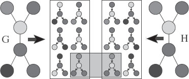
FIGURE 17.3
Graph kernels between two graphs (each color represents a different label). We display all binary 1-tree walks with a specific tree structure, extracted from two simple graphs. The graph kernels are computing and summing the local kernels between all those extracted tree-walks. In the case of the Dirac kernel (hard matching), only one pair of tree-walks is matched (for both labels and structures).

$k_{\alpha ,\beta ,\gamma }^{\mathcal{T}}\left(g,\mathscr{H}\right)={\displaystyle \sum _{T\in {\mathcal{T}}_{\alpha ,\gamma }}{f}_{\lambda ,\nu }\left(T\right)\left\{{\displaystyle \sum _{I\in {\mathcal{J}}_{\beta }\left(T,g\right)}{\displaystyle \sum _{J\in {\mathcal{J}}_{\beta }\left(T,\mathscr{H}\right)}{q}_{T,I,J}\left(g,\mathscr{H}\right)}}\right\}.}$

(17.1)

Details on the efficient computation of the tree-walk kernel are given in the next section. When considering 1-walks (i.e., α = β = 1), and letting the maximal walk length γ tend to +∞, we get back the random walk kernel [12, 14]. If the kernel $q_{T,I,J}\left(g,\mathscr{H}\right)$ has nonnegative values and is equal to 1 if the two tree-walks are equal, it can be seen as a soft matching indicator, and then the kernel simply counts the softly matched tree-walks in the two graphs (see Figure 17.3 for an illustration with hard matching).

We add a nonnegative penalization f_{λ, ν} (T) depending only on the tree structure. Besides the usual penalization of the number of nodes |T|, we also add a penalization of the number of leaf nodes ℓ(T) (i.e., nodes with no children). More precisely, we use the penalization f_λ,ν = λ^|T|ν^ℓ(T). This penalization, suggested by [34], is essential in our situation to prevent trees with nodes of higher degrees from dominating the sum. Yet, we shall most often drop this penalization in subsequent derivations to highlight essential calculations and to keep the notation light.

If q_T,I,J(G, H) is obtained from a positive-definite kernel between (labelled) tree-walks, then $k_{\alpha ,\beta ,\gamma }^{\mathcal{T}}\left(g,\mathscr{H}\right)$ also defines a positive-definite kernel. The kernel $k_{\alpha ,\beta ,\gamma }^{\mathcal{T}}\left(g,\mathscr{H}\right)$ sums the local kernel q_T,I,J(G, H) over all tree-walks of g and $\mathscr{H}$ that share the same tree structure. The number of such matching tree-walks is exponential in the depth γ, thus, in order to deal with potentially deep trees, a recursive definition is needed. The local kernel will depend on the application at hand. In the next sections, we show how one can design meaningful local kernels resp. for region adjacency graphs and point clouds.

17.3  The Region Adjacency Graph Kernel as a Tree-Walk Kernel

We propose to model appearance of images using region adjacency graphs obtained by morphological segmentation. If enough segments are used, i.e., if the image (and hence the objects of interest) is over-segmented, then the segmentation enables us to reduce the dimension of the image while preserving the boundaries of objects. Image dimensionality goes from millions of pixels down to hundreds of segments, with little loss of information. Those segments are naturally embedded in a planar graph structure. Our approach takes into account graph planarity. The goal of this section is to show that one can feed kernel-based learning methods with a kernel measuring appropriate region adjacency graph similarity, called the region adjacency graph kernel, for the purpose of image classification. Note that this kernel was previously referred to as the segmentation graph kernel in the original paper [15].

17.3.1  Morphological Region Adjacency Graphs

Among the many methods available for the segmentation of natural images [35, 36, 37], we chose to use the watershed transform for image segmentation [35], which allows a fast segmentation of large images into a given number of segments. First, given a color image, a grayscale gradient image is computed from oriented energy filters on the LAB representation of the image, with two different scales and eight orientations [38]. Then, the watershed transform is applied to this gradient image, and the number of resulting regions is reduced to a given number p (p = 100 in our experiments) using the hierarchical framework of [35]. We finally obtain p singly connected regions, together with the planar neighborhood graph. An example of segmentation is shown in Figure 17.4.

We have chosen a reasonable value of p because our similarity measure implicitly relies on the fact that images are mostly oversegmented, i.e., the objects of interest may span more than one segment, but very few segments span several objects. This has to be contrasted with the usual (and often unreached) segmentation goal of obtaining one segment per object. In this respect, we could have also used other image segmentation algorithms, such as the Superpixels algorithm [39, 40]. In this section, we always use the same number of segments; a detailed analysis of the effect of choosing a different number of segments, or a number that depends on the given image, is outside the scope of this work.

In this section, images will be represented by a region adjacency graph, i.e., an undirected labelled planar graph, where each vertex is one singly connected region, with edges joining neighboring regions. Since our graph is obtained from neighboring singly connected regions, the graph is planar, i.e., it can be embedded in a plane where no edge intersects [4]. The only property of planar graphs that we are going to use is the fact that for each vertex in the graph, there is a natural notion of cyclic ordering of the vertices. Another typical feature of our graphs is their sparsity: indeed, the degree (number of neighbors) of each node is usually small, and the maximum degree typically does not exceed 10.

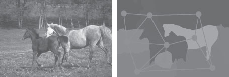
FIGURE 17.4
An example of a natural image (left), and its segmentation mosaic (right) obtained by using the median RGB color in each segmented region. The associated region adjacency graph is depicted in light blue

There are many ways to assign labels to regions, based on shape, color, or texture, leading to highly multivariate labels, which is to be contrasted with the usual application of structured kernels in bioinformatics or natural language processing, where labels belong to a small discrete set. Our family of kernels simply requires a simple kernel k(ℓ, ℓ′) between labels ℓ and ℓ of different regions, which can be any positive semi-definite kernel [1], and not merely a Dirac kernel, which is commonly used for exact matching in bioinformatics applications. We could base such a kernel on any relevant visual information. In this work, we considered kernels between color histograms of each segment, as well as weights corresponding to the size (area) of the segment.

17.3.2  Tree-Walk Kernels on Region Adjacency Graphs

We now make explicit the derivation of tree-walks kernels on region adjacency graphs, in order to highlight the dynamic programming recursion that makes their computation tractable in pratice.

The tree-walk kernel between region adjacency graphs $k_{p,\alpha }\left(g,\mathscr{H}\right)$ is defined as the sum over all tree-walks in G and all tree-walks in $\mathscr{H}$ (sharing the same tree structure) of the products of the local kernels between corresponding individual vertices of the subtree patterns. Note that in the context of exact matching, investigated in [41], this kernel simply counts the number of common subtree-patterns. Note also that, as long as the local kernel is a positive semi-definite kernel, the resulting tree-walk kernel is also an positive semi-definite kernel as well [1].

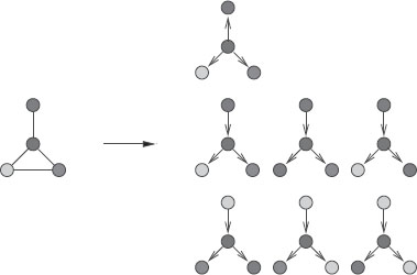
FIGURE 17.5
Examples of tree-walks from a graph. Each color represents a different label.

Local Kernels

In order to apply the tree-walk kernels to region adjacency graphs, we need to specify the kernels involved at the lower level of computation. Here, the local kernels correspond to kernels between segments.

There are plenty of choices for defining relevant features for segment comparisons, ranging from median color to sophisticated local features [42]. We chose to focus on RGB color histograms since previous work [43] thoroughly investigated their relevance for image classification, when used on the whole image without any segmentation. This allows us to fairly evaluate the efficiency of our kernels to make a smart use of segmentations for classification.

Experimental results of kernels between color histograms taken as discretized probability distributions $P={\left(p_i\right)}_{i=1}^N$ were given in [43]. For the sake of simplicity, we shall focus here on the χ²-kernel defined as follows. The symmetric χ²-divergence between two distributions P and Q is defined as

$d_{\chi }^2\left(P,Q\right)=\frac{1}{N}{\displaystyle \sum _{j=1}^N\frac{{\left(p_i-q_i\right)}^2}{p_i+q_i}},$

(17.2)

and the χ²-kernel is defined as

$k_{\chi }\left(P,Q\right)=\exp \left(-\mu d_{\chi }^2\left(P,Q\right)\right),$

(17.3)

with μ a free parameter to be tuned. Following results of [43] and [44], since this kernel is positive semi-definite, it can be used as a local kernel. If we denote P_ℓ the histogram of colors of a region labelled by ℓ, then it defines a kernel between labels as $k\left(\ell ,{\ell }^{\prime }\right)=k_{\chi }\left(P_{\ell },P_{{\ell }^{\prime }}\right)$.

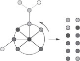
FIGURE 17.6
Enumeration of neighbor intervals of size two.

We need to deal with the too strong diagonal dominance of the obtained kernel matrices, a usual issue with kernels on structured data [3]). We propose to include a constant term λ that controls the maximal value of k(ℓ, ℓ′). We thus use the following kernel

$k\left(\ell ,{\ell }^{\prime }\right)=\lambda \exp \left(-\mu d_{\chi }^2\left(P_{\ell },P_{{\ell }^{\prime }}\right)\right),$

with free parameters λ, μ. Note that, by doing so, we also ensure the positive semidefiniteness of the kernel.

It is natural to give more weight in the overall sum to massive segments than to tiny ones. Hence, we incorporate this into the segment kernel as

$k\left(\ell ,{\ell }^{\prime }\right)=\lambda A_{\ell }^{\gamma }{A}_{{\ell }^{\prime }}^{\gamma }\exp \left(-\mu d_{\chi }^2\left(P_{\ell },P_{{\ell }^{\prime }}\right)\right),$

where A_ℓ is the area of the corresponding region, and γ is an additional free parameter in [0, 1] to be tuned.

Dynamic Programming Recursion

In order to derive an efficient dynamic programming formulation, we now need to restrict the set of subtrees. Indeed, if d is an upper bound on the degrees of the vertices in g and $\mathscr{H}$, then at each depth, the q-ary tree-walk may go through any subsets of size α of the set of neighbors of a given vertex, and thus the matching complexity would be O(d^2α) (O(d^α) for each of the two graphs). We restrict the allowed subsets of neighbors in a tree-walk, by requiring that these subsets are intervals for the natural cyclic ordering of the neighbors of a given vertex (this is possible because the graph is planar). See Figure 17.6 for an enumeration of the intervals of size α = 2. For a given vertex r in g (respectively s in $\mathscr{H}$), we denote by ${\mathcal{A}}_g^{\alpha }\left(r\right)$ (respectively ${\mathcal{A}}_{\mathscr{H}}^{\alpha }\left(s\right)$) the set of nonempty intervals of length at most α around r in g (respectively around s in $\mathscr{H}$). In the rest of the section, we assume that all our subtree patterns (referred to as tree-walks from now on) are restricted to intervals of neighbors. Let $k_{p,\alpha }\left(g,\mathscr{H},r,s\right)$ denote the sum over all tree patterns starting from vertex r in g and s in $\mathscr{H}$.

The following result shows that the recursive dynamic programming formulation that allows us to efficiently compute tree-walk kernels. In the case of the tree-walk kernel for region adjacency graphs, the final kernel writes as follows

$k\left(g,\mathscr{H}\right)={\displaystyle \sum _{r\in {\mathcal{V}}_g,s\in {\mathcal{V}}_{\mathscr{H}}}{k}_{p,\alpha }\left(g,\mathscr{H},r,s\right)}.$

(17.4)

Assuming equal size intervals Card(A) = Card(B), the kernel values $k_{p,\alpha }\left(g,\mathscr{H},r,s\right)$ can be recursively computed through

$k_{p,\alpha }\left(g,\mathscr{H},r,s\right)=k\left({\ell }_g\left(r\right),{\ell }_{\mathscr{H}}\left(s\right)\right){\displaystyle \sum _{A\in {\mathcal{A}}_g^{\alpha }\left(r\right),B\in {\mathcal{A}}_{\mathscr{H}}^{\alpha }\left(s\right)}{\displaystyle \prod _{r^{\prime }\in A,s^{\prime }\in B}{k}_{p-1,\alpha \left(g,\mathscr{H},r^{\prime },s^{\prime }\right)}.}}$

(17.5)

The above equation defines a dynamic programming recursion that allows us to efficiently compute the values of $k_{p,\alpha }\left(g,\mathscr{H},\cdot ,\cdot \right)$ from p = 1 to any desired p. We first compute $k_{1,\alpha }\left(g,\mathscr{H},\cdot ,\cdot \right)$, using that $k\left(g,\mathscr{H},r,s\right)=k\left({\ell }_g\left(r\right),{\ell }_{\mathscr{H}}\left(s\right)\right)$ for r a segment of g and s a segment of $\mathscr{H}$. Then $k_{2,\alpha }\left(g,\mathscr{H},\cdot ,\cdot \right)$ can be computed from $k_{1,\alpha }\left(g,\mathscr{H},\cdot ,\cdot \right)$ using (17.5) with p = 2. And so on. Finally, note that when α = 1 (intervals of size 1), the tree-walk kernel reduces to the walk kernel [12].

Running Time Complexity

Given labelled graphs g and $\mathscr{H}$ with n_g and $n_{\mathscr{H}}$ vertices each and maximum degrees d_g and $d_{\mathscr{H}}$, we assume that the kernel between labels k(ℓ, ℓ′) can be computed in constant time. Hence, the total cost of computing $k\left({\ell }_g\left(r\right),{\ell }_{\mathscr{H}}\left(s\right)\right)$ for all $r\in {\mathcal{V}}_g$ and $s\in {\mathcal{V}}_{\mathscr{H}}$ is $O\left(n_g{n}_{\mathscr{H}}\right)$.

For walk kernels, the complexity of each recursion is $O\left(d_g{d}_{\mathscr{H}}\right)$. Thus, computation of all q-th walk kernels for $q⩽p$ needs $O\left(p{d}_g{d}_{\mathscr{H}}{n}_g{n}_{\mathscr{H}}\right)$ operations.

For tree-walk kernels, the complexity of each recursion is $O\left({\alpha }^2{d}_g{d}_{\mathscr{H}}\right)$. Therefore, computation of all q-th α-ary tree walk kernels for q ⩽ p needs $O\left(p{\alpha }^2{d}_g{d}_{\mathscr{H}}{n}_g{n}_{\mathscr{H}}\right)$ operations, i.e., leading to polynomial-time complexity.

We now pause in the exposition of tree-walk kernels applied to region adjacency graphs, and move on to tree-walk kernels applied to point clouds. We shall get back to tree-walk kernels on region adjacency graphs in Section 17.5.

17.4  The Point Cloud Kernel as a Tree-Walk Kernel

We propose to model shapes of images using point clouds. Indeed, we assume that each point cloud has a graph structure (most often a neighborhood graph).Then, our graph kernels consider all partial matches between two neighborhood graphs and sum over those. However, the straightforward application of graph kernels poses a major problem: in the context of computer vision, substructures correspond to matched sets of points, and dealing with local invariances by rotation and/or translation necessitates the use of a local kernel that cannot be readily expressed as a product of separate terms for each pair of points, and the usual dynamic programming and matrix inversion approaches cannot then be directly applied. We shall assume that the graphs have no self-loops. Our motivating examples are line drawings, where $\mathcal{A}={ℝ}^2$ (i.e., the position is itself also an attribute). In this case, the graph is naturally obtained from the drawings by considering 4-connectivity or 8-connectivity [25]. In other cases, graphs can be easily obtained from nearest-neighbor graphs.

We show here how to design a local kernel that is not fully factorized but can be instead factorized according to the graph underlying the substructure. This is naturally done through probabilistic graphical models and the design of positive-definite kernels for covariance matrices that factorize on probabilistic graphical models. With this novel local kernel, we derive new polynomial time dynamic programming recursions.

17.4.1  Local Kernels

The local kernel is used between tree-walks that can have large depths (note that everything we propose will turn out to have linear time complexity in the depth γ). Recall here that, given a tree structure T and consistent labellings $I\in {\mathcal{J}}_{\beta }\left(T,G\right)$ and $J\in {\mathcal{J}}_{\beta }\left(T,H\right)$, the quantity q_T,I,J(G, H) denotes the value of the local kernel between two tree-walks defined by the same structure T and labellings I and J. We use the product of a kernel for attributes and a kernel for positions. For attributes, we use the following usual factorized form $q_{\mathcal{A}}\left(a\left(I\right),b\left(J\right)\right)={\displaystyle {\prod }_{p=1}^{\left|I\right|}{k}_{\mathcal{A}}\left(a\left(I_p\right),b\left(J_p\right)\right)}$, where $k_{\mathcal{A}}$ is a positive-definite kernel on $\mathcal{A}\times \mathcal{A}$. This allows the separate comparison of each matched pair of points and efficient dynamic programming recursions. However, for our local kernel on positions, we need a kernel that jointly depends on the whole vectors x(I) ∈ X^|I| and y(J) ∈ X^|J|, and not only on the p pairs (x(I_p), y(J_p)). Indeed, we do not assume that the pairs are registered; i.e., we do not know the matching between points indexed by I in the first graph and the ones indexed by J in the second graph.

We shall focus here on $\text{X}\text{=}{ℛ}^d$ and translation-invariant local kernels, which implies that the local kernel for positions may only depend on differences x(i) − x(i′) and y(j) − y(j′) for (i, i′) ∈ I × I and (j, j′) ∈ J × J. We further reduce these to kernel matrices corresponding to a translation-invariant positive-definite kernel k_X(x₁ − x₂). Depending on the application, k_X may or may not be rotation invariant. In experiments, we use the rotation-invariant Gaussian kernel of the form k_X(x₁, x₂) = exp(−υ║x₁ − x₂║²).

Thus, we reduce the set of all positions in X^|V| and X^|W| to full kernel matrices $K\in {ℛ}^{\left|V\right|\times \left|V\right|}$ and $L\in {ℛ}^{\left|W\right|\times \left|W\right|}$ for each graph, defined as K(υ, υ′) = k_X(x(υ) − x(υ′)) (and similarly for L). These matrices are by construction symmetric positive semi-definite and, for simplicity, we assume that these matrices are positive-definite (i.e., invertible), which can be enforced by adding a multiple of the identity matrix. The local kernel will thus only depend on the submatrices K_I = K_I,I and L_J = L_J,J, which are positive-definite matrices. Note that we use kernel matrices K and L to represent the geometry of each graph, and that we use a positive-definite kernel on such kernel matrices.

We consider the following positive-definite kernel on positive matrices K and L, the (squared) Bhattacharyya kernel $k_{ℬ}$, defined as [45]:

$k_{ℬ}\left(K,L\right)={\left|K\right|}^{1/2}{\left|L\right|}^{1/2}{\left|\frac{K+L}{2}\right|}^{-1},$

(17.6)

where |K| denotes the determinant of K.

By taking the product of the attribute-based local kernel and the position-based local kernel, we get the following local kernel $q_{T,I,J}^0\left(G,H\right)=k_{ℬ}{\left(K_I,L_J\right)}_{q_{\mathcal{A}}}\left(a\left(I\right),b\left(J\right)\right)$. However, this local kernel $q_{T,I,J}^0\left(G,H\right)$ does not yet depend on the tree structure T and the recursion may be efficient only if $q_{T,I,J}^0\left(G,H\right)$ can be computed recursively. The factorized term $q_{\mathcal{A}}\left(a\left(I\right),b\left(J\right)\right)$ is not an issue. However, for the term $k_{ℬ}\left(K_I,L_J\right)$, we need an approximation based on T. As we show in the next section, this can be obtained by a factorization according to the appropriate probabilistic graphical model; i.e., we will replace each kernel matrix of the form K_I by a projection onto a subset of kernel matrices, which allows efficient recursions.

17.4.2  Positive Matrices and Probabilistic Graphical Models

The main idea underlying the factorization of the kernel is to consider symmetric positive-definite matrices as covariance matrices and to look at probabilistic graphical models defined for Gaussian random vectors with those covariance matrices. The goal of this section is to show that by appropriate probabilistic graphical model techniques, we can design properly factorized approximations of Equation 17.6, namely, through Equations 17.11 and 17.12.

More precisely, we assume that we have n random variables Z₁,…, Z_n with probability distribution p(z) = p(z₁,…, z_n). Given a kernel matrix K (in our case defined as K_ij = exp(−υ║x_i − x_j║²), for positions x₁,…, x_n), we consider jointly Gaussian distributed random variables Z₁,…, Z_n such that Cov(Z_i, Z_j) = K_ij. In this section, with this identification, we consider covariance matrices as kernel matrices, and vice versa.

Probabilistic Graphical Models and Junction Trees

Probabilistic graphical models provide a flexible and intuitive way of defining factorized probability distributions. Given any undirected graph Q with vertices in {1,…, n}, the distribution p(z) is said to factorize in Q if it can be written as a product of potentials over all cliques (completely connected subgraphs) of the graph Q. When the distribution is Gaussian with covariance matrix $K\in {ℛ}^{n\times n}$, the distribution factorizes if and only if (K⁻¹)_ij = 0 for each (i, j) that is not an edge in Q [46].

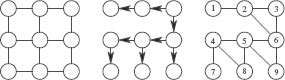
FIGURE 17.7
(Left) original graph, (middle) a single extracted tree-walk, (right) decomposable graphical model Q₁(T) with added edges in red. The junction tree is a chain composed of the cliques {1, 2}, {2, 3, 6}, {5, 6, 9}, {4, 5, 8}, {4, 7}.

In this section, we only consider decomposable probabilistic graphical models, for which the graph Q is triangulated (i.e., there exists no chordless cycle of length strictly larger than 3). In this case, the joint distribution is uniquely defined from its marginals p_C(z_C) on the cliques C of the graph Q. That is, if $\mathcal{C}\left(Q\right)$ is the set of maximal cliques of Q, we can build a tree of cliques, a junction tree, such that

$p\left(z\right)=\frac{{\displaystyle {\prod }_{C\in \mathcal{C}\left(Q\right)}{p}_C\left(z_C\right)}}{{\displaystyle {\prod }_{C,C^{\prime }\in \mathcal{C}\left(Q\right),C~C^{\prime }}{p}_{C\cap C^{\prime }}\left(z_{C\cap C^{\prime }}\right)}}.$

Figure 17.7 shows an example of a probabilistic graphical model and a junction tree. The sets C ∩ C′ are usually referred to as separators, and we let $\mathcal{S}\left(Q\right)$ denote the set of such separators. Note that for a zero mean normally distributed vector, the marginals p_C (z_C) are characterized by the marginal covariance matrix K_C = K_C,C. Projecting onto a probabilistic graphical model will preserve the marginal over all maximal cliques, and thus preserve the local kernel matrices, while imposing zeros in the inverse of K.

Probabilistic Graphical Models and Projections

We let Π_Q(K) denote the covariance matrix that factorizes in Q which is closest to K for the Kullback-Leibler divergence between normal distributions. We essentially replace K by Π_Q(K). In other words, we project all our covariance matrices onto a probabilistic graphical model, which is a classical tool in statistics [46, 47]. We leave the study of the approximation properties of such a projection (i.e., for a given K, how dense the graph should be to approximate the full local kernel correctly?) to future work—see, e.g., [48] for related results.

Practically, since our kernel on kernel matrices involves determinants, we simply need to compute |Π_Q(K)| efficiently. For decomposable probabilistic graphical models, Π_Q(K) can be obtained in closed form [46] and its determinant has the following simple expression:

$\log \left|{\displaystyle \prod {}_Q\left(K\right)}\right|={\displaystyle \sum _{C\in \mathcal{C}\left(Q\right)}\log \left|K_C\right|-{\displaystyle \sum _{S\in \mathcal{S}\left(Q\right)}\log \left|K_S\right|.}}$

(17.7)

The determinant |Π_Q(K)| is thus a ratio of terms (determinants over cliques and separators), which will restrict the applicability of the projected kernels (see Proposition 1). In order to keep only products, we consider the following equivalent form: if the junction tree is rooted (by choosing any clique as the root), then for each clique but the root, a unique parent clique is defined, and we have

$\log \left|{\displaystyle \prod {}_Q\left(K\right)}\right|={\displaystyle \sum _{C\in \mathcal{C}\left(Q\right)}\log \left|K_{C|p_Q\left(C\right)}\right|,}$

(17.8)

where p_Q(C) is the parent clique of Q (and Ø for the root clique) and the conditional covariance matrix is defined, as usual, as

$K_{C|p_Q\left(C\right)}=K_{C,C}-K_{C,p_Q\left(C\right)}{K}_{p_Q\left(C\right),p_Q\left(C\right)}^{-1}{K}_{p_Q\left(C\right),C}.$

(17.9)

Probabilistic Graphical Models and Kernels

We now propose several ways of defining a kernel adapted to probabilistic graphical models. All of them are based on replacing determinants |M| by |Π_Q(M)|, and their different decompositions in Equations 17.7 and 17.8. Simply using Equation 17.7, we obtain the similarity measure:

$k_{ℬ,0}^Q\left(K,L\right)={\displaystyle \prod _{C\in \mathcal{C}\left(Q\right)}{k}_{ℬ}\left(K_C,L_C\right)}{\displaystyle \prod _{S\in \mathcal{S}\left(Q\right)}{k}_{ℬ}{\left(K_S,L_S\right)}^{-1}.}$

(17.10)

This similarity measure turns out not to be a positive-definite kernel for general covariance matrices.

Proposition 1

For any decomposable model Q, the kernel $k_{ℬ,0}^Q$ defined in Equation 17.10 is a positive-definite kernel on the set of covariance matrices K such that for all separators $S\in \mathcal{S}\left(Q\right)$, K_S,S = I. In particular, when all separators have cardinal one, this is a kernel on correlation matrices.

In order to remove the condition on separators (i.e., we want more sharing between cliques than through a single variable), we consider the rooted junction tree representation in Equation 17.8. A straightforward kernel is to compute the product of the Bhattacharyya kernels $k_{ℬ}\left(K_{C|p_Q\left(C\right)},L_{C|p_Q\left(C\right)}\right)$ for each conditional covariance matrix. However, this does not lead to a true distance on covariance matrices that factorize on Q because the set of conditional covariance matrices do not characterize entirely those distributions. Rather, we consider the following kernel:

$k_{ℬ}^Q\left(K,L\right)={\displaystyle {\prod }_{C\in \mathcal{C}\left(Q\right)}{k}_{ℬ}^{C|p_Q\left(C\right)}}\left(K,L\right);$

(17.11)

for the root clique, we define $k_{ℬ}^{R|\varnothing }\left(K,L\right)=k_{ℬ}\left(K_R,L_R\right)$ and the kernels $k_{ℬ}^{C|p_Q\left(C\right)}\left(K,L\right)$, are defined as kernels between conditional Gaussian distributions of Z_C given Z_pQ(C). We use

$k_{ℬ}^{C|p_Q\left(C\right)}\left(k,L\right)=\frac{{\left|K_{C|p_Q\left(C\right)}\right|}^{1/2}{\left|L_{C|p_Q\left(C\right)}\right|}^{1/2}}{\left|\frac{1}{2}{K}_{C|p_Q\left(C\right)}+\frac{1}{2}{L}_{C|p_Q\left(C\right)}+M{M}^{\top }\right|},$

(17.12)

where the additional term M is equal to $\frac{1}{2}\left(K_{C,p_Q\left(C\right)}{K}_{p_Q\left(C\right)}^{-1}-L_{C,p_Q\left(C\right)}{L}_{p_Q\left(C\right)}^{-1}\right)$. This exactly corresponds to putting a prior with identity covariance matrix on variables Z_pQ(C) and considering the kernel between the resulting joint covariance matrices on variables indexed by (C, p_Q(C)). We now have a positive-definite kernel on all covariance matrices:

Proposition 2

For any decomposable model Q, the kernel $k_{ℬ}^Q\left(K,L\right)$ defined in Equation 17.11 and Equation 17.12 is a positive-definite kernel on the set of covariance matrices.

Note that the kernel is not invariant by the choice of the particular root of the junction tree. However, in our setting, this is not an issue because we have a natural way of rooting the junction trees (i.e, following the rooted tree-walk). Note that these kernels could be useful in domains other than computer vision.

In the next derivations, we will use the notation $k_{ℬ}^{I_1|I_2,J_1|J_2}\left(K,L\right)$ for |I₁| = |I₂| and |J₁| = |J₂| to denote the kernel between covariance matrices K_I1∪I2 and L_I1∪I2 adapted to the conditional distributions I₁|I₂ and J₁|J₂, defined through Equation 17.12.

Choice of Probabilistic Graphical Models

Given the rooted tree structure T of a β-tree-walk, we now need to define the probabilistic graphical model Q_β(T) that we use to project our kernel matrices. A natural candidate is T itself. However, as shown later, in order to compute efficiently the kernel we simply need that the local kernel is a product of terms that only involve a node and its β-descendants. The densest graph (remember that denser graphs lead to better approximations when projecting onto the probabilistic graphical model) we may use is the following: we define Q_β(T) such that for all nodes in T, the node together with all its β-descendants form a clique, i.e., a node is connected to its β-descendants and all β-descendants are also mutually connected (see Figure 17.7, for example, for β = 1): the set of cliques is thus the set of families of depth β + 1 (i.e., with β + 1 generations). Thus, our final kernel is

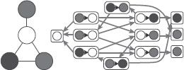
FIGURE 17.8
(Left) undirected graph G, (right) graph G_1,2.

$k_{\alpha ,\beta ,\gamma }^{\mathcal{T}}\left(G,H\right)={\displaystyle \sum _{T\in {\mathcal{T}}_{\alpha ,\gamma }}{f}_{\lambda ,\nu }\left(T\right)}\{{\displaystyle \sum _{I\in {\mathcal{J}}_{\beta }\left(T,G\right)}{\displaystyle \sum _{J\in {\mathcal{J}}_{\beta }\left(T,H\right)}{k}_{ℬ}^{Q_{\beta }\left(T\right)}\left(K_I,L_J\right)q_{\mathcal{A}}\left(a\left(I\right),b\left(J\right)\right)}}).$

The main intuition behind this definition is to sum local similarities over all matching subgraphs. In order to obtain a tractable formulation, we simply needed (a) to extend the set of subgraphs (to tree-walks of depth γ) and (b) to factorize the local similarities along the graphs. We now show how these elements can be combined to derive efficient recursions.

17.4.3  Dynamic Programming Recursions

In order to derive dynamic programming recursions, we follow [34] and rely on the fact that α-ary β-tree-walks of G can essentially be defined through 1-tree-walks on the augmented graph of all rooted subtrees of G of depth at most β and arity less than α. Recall that the arity of a tree is the maximum number of children of the root and internal vertices of the tree. We thus consider the set V_{α, β} of noncomplete rooted (unordered) subtrees of G = (V, E), of depths less than β and arity less than α. Given two different rooted unordered labelled trees, they are said to be equivalent (or isomorphic) if they share the same tree structure, and this is denoted ~_t.

On this set V_α,β, we define a directed graph with edge set E_α,β as follows: R₀ ∈ V_α,β is connected to R₁ ∈ V_α,β if “the tree R₁ extends the tree R₀ one generation further”, i.e., if and only if (a) the first β − 1 generations of R₁ are exactly equal to one of the complete subtrees of R₀ rooted at a child of the root of R₀, and (b) the nodes of depth β of R₁ are distinct from the nodes in R₀. This defines a graph G_α,β = (V_α,β, E_α,β) and a neighborhood ${\mathcal{N}}_{G_{\alpha ,\beta }}\left(R\right)$ for R ∈ V_α,β (see Figure 17.8 for an example). Similarly, we define a graph H_α,β = (W_α,β, F_α,β) for the graph H. Note that when α = 1, V_1,β is the set of paths of length less than or equal to β.

For a β-tree-walk, the root with its β-descendants must have distinct vertices and thus corresponds exactly to an element of V_α,β. We denote $k_{\alpha ,\beta ,\gamma }^{\mathcal{T}}\left(G,H,R_0,S_0\right)$ the same kernel as defined in Equation 17.4.2, but restricted to tree-walks that start respectively with R₀ and S₀. Note that if R₀ and S₀ are not equivalent, then $k_{\alpha ,\beta ,\gamma }^{\mathcal{T}}\left(G,H,R_0,S_0\right)=0$.

Denote ρ(S) the root of a subtree S. We obtain the following recursion between depths γ and depth γ − 1, for all R₀ ∈ V_α,β and and S₀ ∈ W_α,β such that R₀ ~_t S₀:

$k_{\alpha ,\beta ,\gamma }^{\mathcal{T}}\left(G,H,R_0,S_0\right)=k_{\alpha ,\beta ,\gamma -1}^{\mathcal{T}}\left(G,H,R_0,S_0\right)+{ℛ}_{\alpha ,\beta ,\gamma -1}^{\mathcal{T}},$

(17.13)

where $R_{\alpha ,\beta ,\gamma -1}^{\mathcal{T}}$ is given by

$\begin{array}{c}{ℛ}_{\alpha ,\beta ,\gamma -1}^{\mathcal{T}}={\displaystyle \sum _{p=1}^{\alpha }{\displaystyle \sum _{\begin{array}{c}{R}_1,\mathrm{\dots },R_p\in {\mathcal{N}}_{G_{\alpha ,\beta }}\left(R_0\right)\\ R_1,\mathrm{\dots },R_p\text{disjoint}\end{array}}{\displaystyle \sum _{\begin{array}{c}{S}_1,\mathrm{\dots },S_p\in {\mathcal{N}}_{H_{\alpha ,\beta }}\left(S_0\right)\\ S_1,\mathrm{\dots },S_p\text{disjoint}\end{array}}\cdots }}}\\ \left[\lambda {\displaystyle \prod _{i=1}^p{k}_A\left(a\left(\rho \left(R_i\right)\right),b\left(\rho \left(S_i\right)\right)\right)}\frac{k_{ℬ}^{{\cup }_{i=1}^p{R}_i|R_0,{\cup }_{i=1}^p{S}_i|S_0}\left(K,L\right)}{{\displaystyle {\prod }_{i=1}^p{k}_{ℬ}^{R_i,S_i}\left(K,L\right)}}\left({\displaystyle \prod _{i=1}^p{k}_{\alpha ,\beta ,\gamma -1}^{\mathcal{T}}}\left(G,H,R_i,S_i\right)\right)\right].\end{array}$

(17.14)

Note that if any of the trees R_i is not equivalent to S_i, it does not contribute to the sum. The recursion is initialized with

$k_{\alpha ,\beta ,\gamma }^{\mathcal{T}}\left(G,H,R_0,S_0\right)={\lambda }^{\left|R_0\right|}{\nu }^{\ell \left(R_0\right)}{q}_{\mathcal{A}}\left(a\left(R_0\right),b\left(S_0\right)\right)k_{ℬ}\left(K_{R_0},L_{S_0}\right)$

(17.15)

while the final kernel is obtained by summing over all R₀ and S₀, i.e., $k_{\alpha ,\beta ,\gamma }^{\mathcal{T}}\left(G,H\right)={\displaystyle \sum {}_{R_0{~}_t{S}_0}{k}_{\alpha ,\beta ,\gamma }^{\mathcal{T}}\left(G,H,R_0,S_0\right)}$.

Computational Complexity

The above equations define a dynamic programming recursion that allows us to efficiently compute the values of $k_{\alpha ,\beta ,\gamma }^{\mathcal{T}}\left(G,H,R_0,S_0\right)$ from γ = 1 to any desired γ. We first compute $k_{\alpha ,\beta ,1}^{\mathcal{T}}\left(G,H,R_0,S_0\right)$ using Equation 17.15. Then $k_{\alpha ,\beta ,2}^{\mathcal{T}}\left(G,H,R_0,S_0\right)$ can be computed from $k_{\alpha ,\beta ,1}^{\mathcal{T}}\left(G,H,R_0,S_0\right)$ using Equation 17.13 with γ = 2. And so on.

The complexity of computing one kernel between two graphs is linear in γ (the depth of the tree-walks), and quadratic in the size of V_α,β and W_α,β. However, those sets may have exponential size in β and α in general (in particular, if graphs are densely connected). And thus, we are limited to small values (typically α ⩽ 3 and β ⩽ 6), which are sufficient for satisfactory classification performance (in particular, higher β or α do not necessarily mean better performance). Overall, one can deal with any graph size, as long as the “sufficient statistics” (i.e., the unique local neighborhoods in V_α,β) are not too numerous.

For example, for the handwritten digits we use in experiments, the average number of nodes in the graphs is 18 ± 4, while the average cardinality of V_α,β and running times¹ for one kernel evaluation are, for walk kernels of depth 24: |V_α,β| = 36, time = 2 ms (α = 1, β = 2), |V_α,β| = 37, time = 3 ms (α = 1, β = 4); and for tree kernels: |V_α,β| = 56, time = 25 ms (α = 2, β = 2), |V_α,β| = 70, time = 32 ms (α = 2, β = 4).

Finally, we may reduce the computational load by considering a set of trees of smaller arity in the previous recursions; i.e., we can consider V_1,β instead of V_α,β with tree kernels of arity α > 1.

17.5  Experimental Results

We present here experimental results of tree-walk kernels, respectively, on: (i) region adjacency graphs for object categorization and natural image classification, and (ii) point clouds for handwritten digits classification.

17.5.1  Application to Object Categorization

We have tested our kernels on the task of object categorization (Coil100 dataset), and natural image classification (Corel14 dataset) both in fully supervised and in semi supervised settings.

Experimental Setting

Experiments have been carried out on both Corel14 [22] and Coil100 datasets. Our kernels were put to the test step by step, going from the less sophisticated version to the most complex one. Indeed, we compared on a multi-class classification task performances of the usual histogram kernel (H), the walk-based kernel (W), the tree-walk kernel (TW), the weighted-vertex tree-walk kernel (wTW), and the combination of the above by multiple kernel learning (M). We report here their performances averaged in an outer loop of 5-fold cross-validation. The hyperparameters are tuned in an inner loop in each fold by 5-fold cross-validation (see in the sequel for further details). Coil100 consists in a database of 7200 images of 100 objects in a uniform background, with 72 images per object. Data are color images of the objects taken from different angles, with steps of 5 degrees. Corel14 is a database of 1400 natural images of 14 different classes, which are usually considered much harder to classify. Each class contains 100 images, with a non-negligible proportion of outliers.

Feature Extraction

Each image’s segmentation outputs a labelled graph with 100 vertices, with each vertex labelled with the RGB-color histogram within each corresponding segment. We used 16 bins per dimension, as in [43], yielding 4096-dimensional histograms. Note that we could use LAB histograms as well. The average vertex degree was around 3 for Coil100 and 5 for Corel14. In other words, region adjacency graphs are very sparsely connected.

Free Parameter Selection

For the multi-class classification task, the usual SVM classifier was used in a one-versus-all setting [1]. For each family of kernels, hyper-parameters corresponding to kernel design and the SVM regularization parameter C were learned by crossvalidation, with the following usual machine learning procedure: we randomly split the full dataset in 5 parts of equal size, then we consider successively each of the 5 parts as the testing set (the outer testing fold), learning being performed on the four other parts (the outer training fold). This is in contrast to other evaluation protocols. Assume instead one is trying out different values of the free parameters on the outer training fold, computing the prediction accuracy on the corresponding testing fold, repeating five times for each of the five outer folds, and compute average performance. Then assume one selects the best hyper-parameter and report its performance. A major issue with such a protocol is that it leads to an optimistic estimation of the prediction performance [49].

It is preferable to consider each outer training fold, and split those into 5 equal parts, and learn the hyper-parameters using cross-validation on those inner folds, and use the resulting parameter, train on the full outer training fold with this set of hyperparameters (which might be different for each outer fold), and test on the outer testing fold. The prediction accuracies that we report (in particular in the boxplots of Figure 17.11) are the prediction accuracies on the outer testing folds. This two-stage approach leads to more numerous estimations of SVM parameters but provides a fair evaluation of performance.

In order to choose the values of the free parameters, we use values of free parameters on the finite grid in Figure 17.9.

The respective performances in average test error rates (on the five testing outer folds) in multi-class classification of the different kernels are listed in Figure 17.10. See Figure 17.11 for corresponding boxplots for the Corel14 dataset.

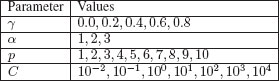
FIGURE 17.9
Range of values of the free parameters.

FIGURE 17.10
Best test error performances of histogram, walk, tree-walk, tree-walk with weighted segments, kernels

Corel14 dataset

We have compared test error rate performances of SVM-based multi-class classification with histogram kernel (H), walk kernel (W), tree-walk kernel (TW), and the tree-walk kernel with weighted segments (wTW). Our methods, i.e., TW and wTW, clearly outperform global histogram kernels and simple walk kernels. This corroborates the efficiency of tree-walk kernels in capturing the topological structure of natural images. Our weighting scheme also seems to be reasonable.

Multiple Kernel Learning

We first tried the combination of histogram kernels with walk-based kernels, which did not yield significant performance enhancement. This suggests that histograms do not carry any supplemental information over walk-based kernels: the global histogram information is implicitly retrieved in the summation process of walk-based kernels.

We ran the multiple kernel learning (MKL) algorithm of [50] with 100 kernels (i.e., a rough subset of the set of all parameter settings with parameters taken values detailed in Figure 17.9). As seen in Figure 17.11, the performance increases as expected. It is also worth looking at the kernels that were selected. We here give results for one of the five outer cross-validation folds, where 5 kernels were selected, as displayed in Figure 17.12.

It is worth noting that various values of γ, α, and p are selected, showing that each setting may indeed capture different discriminative information from the segmented images.

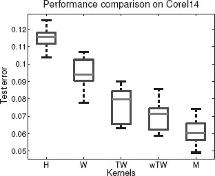
FIGURE 17.11
Test errors for supervised multi-class classification on Corel14, for Histogram, Walk, Tree-Walk, weighted Tree-Walk, kernels, and optimal Multiple kernel combination.

FIGURE 17.12
Weight η of the kernels with the largest magnitude (see [50] for details on normalization of η).

Semi-Supervised Classification

Kernels allow us to tackle many tasks, from unsupervised clustering to multi-class classification and manifold learning [1]. To further explore the expressiveness of our region adjacency graph kernels, we give below the evolution of test error performances on Corel14 dataset for multi-class classification with 10% labelled examples, 10% test examples, and an increasing amount ranging from 10% to 80% of unlabelled examples. Indeed, all semi-supervised algorithms derived from statistically consistent supervised ones see their test errors falling down as the number of labelled examples is increased and the number of unlabelled examples kept constant. However, such experimental convergence of the test errors as the number of labelled examples is kept fixed and the number of unlabelled ones is increased is much less systematic [51]. We used the publicly available code for the low-density separation (LDS) algorithm of [51], since it achieved good performance on the Coil100 image dataset.

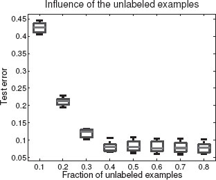
FIGURE 17.13
Test error evolution for semi-supervised multi-class classification as the number of unlabelled examples increases.

Since we are more interested in showing the flexibility of our approach than the semi-supervised learning problem in general, we simply took as a kernel the optimal kernel learned on the whole supervised multi-classification task by the multiple kernel learning method. Although this may lead to a slight overestimation of the prediction accuracies, this allowed us to bypass the kernel selection issue in semisupervised classification, which still remains unclear and under active investigation. For each amount of unlabelled examples, as an outer loop we randomly selected 10 different splits into labelled and unlabelled examples. As an inner loop we optimized the hyperparameters, namely the regularization parameter C and ρ the cluster squeezing parameter (see [51] for details), by leave-one-out cross-validation. The boxplots in Figure 17.13 shows the variability of performances within the outer loop. Keeping in mind that the best test error performance on the Corel14 dataset of histogram kernels is around 10% for completely supervised multi-class classification, the results are very promising; we see that our kernel reaches this level of performance for as little as 40% unlabelled examples and 10% labelled examples.

We now present the experimental results obtained with tree-walk kernels on point clouds in a character recognition task.

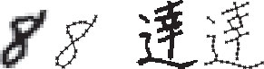
FIGURE 17.14
For digits and Chinese characters: (left) original characters, (right) thinned and subsampled characters.

17.5.2  Application to Character Recognition

We have tested our kernels on the task of isolated handwritten character recognition, handwritten arabic numerals (MNIST dataset), and Chinese characters (ETL9B dataset).

17.5.3  Experimental Setting

We selected the first 100 examples for the ten classes in the MNIST dataset, while for the ETL9B dataset, we selected the five hardest classes to discriminate among 3,000 classes (by computing distances between class means) and then selected the first 50 examples per class. Our learning task is to classify those characters; we use a one-versus-rest multiclass scheme with 1-norm support vector machines (see, e.g., [1]).

Feature Extraction

We consider characters as drawings in ${ℛ}^2$, which are sets of possibly intersecting contours. Those are naturally represented as undirected planar graphs. We have thinned and subsampled uniformly each character to reduce the sizes of the graphs (see two examples in Figure 17.14). The kernel on positions is $k_{\mathcal{X}}\left(x,y\right)=\exp \left(-\tau {\Vert x-y\Vert }^2\right)+\kappa \delta \left(x,y\right)$, but could take into account different weights on horizontal and vertical directions. We add the positions from the center of the bounding box as features, to take into account the global positions, i.e., we use $k_{\mathcal{A}}\left(x,y\right)=\exp \left(-\upsilon {\Vert x-y\Vert }^2\right)$. This is necessary because the problem of handwritten character recognition is not globally translation invariant.

Free Parameter Selection

The tree-walk kernels on point clouds have the following free parameters (shown with their possible values): arity of tree-walks (α = 1, 2), order of tree-walks (β = 1, 2, 4, 6), depth of tree-walks (γ = 1, 2, 4, 8, 16, 24), penalization on number of nodes (λ = 1), penalization on number of leaf nodes (ν = .1, .01), bandwidth for kernel on positions (τ = .05, .01, .1), ridge parameter (κ = .001), and bandwidth for kernel on attributes (υ = .05, .01, .1).

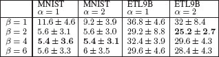
FIGURE 17.15
Error rates (multiplied by 100) on handwritten character classification tasks.

The first two sets of parameters (α, β, γ, λ, ν) are parameters of the graph kernel, independent of the application, while the last set (τ, k, ν) are parameters of the kernels for attributes and positions. Note that with only a few important scale parameters (τ and ν), we are able to characterize complex interactions between the vertices and edges of the graphs. In practice, this is important to avoid considering many more distinct parameters for all sizes and topologies of subtrees. In experiments, we performed two loops of 5-fold cross-validation: in the outer loop, we consider 5 different training folds with their corresponding testing folds. On each training fold, we consider all possible values of α and β. For all of those values, we select all other parameters (including the regularization parameters of the SVM) by 5-fold crossvalidation (the inner folds). Once the best parameters are found only by looking only at the training fold, we train on the whole training fold and test on the testing fold. We output the means and standard deviations of the testing errors for each testing fold.

We show in Figure 17.15 the performance for various values of α and β. We compare those favorably to three baseline kernels with hyperparameters learned by cross-validation in the same way: (a) the Gaussian-RBF kernel on the vectorized original images, which leads to testing errors of 11.6 ± 5.4% (MNIST) and 50.4 ± 6.2% (ETL9B); (b) the regular random walk kernel that sums over all walk lengths, which leads to testing errors of 8.6 ± 1.3% (MNIST) and 34.8 ± 8.4% (ETL9B); and (c) the pyramid match kernel [52], which is commonly used for image classification and leads here to testing errors of 10.8 ± 3.6% (MNIST) and 45.2 ± 3.4% (ETL9B). These results show that our family of kernels, which use the natural structure of line drawings, are outperforming other kernels on structured data (regular random walk kernel and pyramid match kernel) as well as the “blind” Gaussian-RBF kernel, which does not take into account explicitly the structure of images but still leads to very good performance with more training data [9]. Note that for Arabic numerals, higher arity does not help, which is not surprising since most digits have a linear structure (i.e, graphs are chains). On the contrary, for Chinese characters, which exhibit higher connectivity, best performance is achieved for binary tree-walks.

17.6  Conlusion

We have presented a family of kernels for computer vision tasks, along with two instantiations of these kernels: (i) tree-walk kernels for region adjacency graphs, and (ii) tree-walk kernels for point clouds. For (i), we have showed how one can efficiently compute kernels in polynomial time with respect to the size of the region adjacency graphs and their degrees. For (ii), we proposed an efficient dynamic programming algorithm using a specific factorized form for the local kernels between tree-walks, namely a factorization on a properly defined probabilistic graphical model. We have reported applications to object categorization and natural image classification, as well as handwritten character recognition, where we showed that the kernels were able to capture the relevant information to allow good predictions from few training examples.

17.7  Acknowledgments

This work was partially supported by grants from the Agence Nationale de la Recherche (MGA Project) and from the European Research Council (SIERRA Project), and the PASCAL 2 Network of Excellence.

Bibliography

[1]  J. Shawe-Taylor and N. Cristianini, Kernel Methods for Pattern Analysis. Cambridge Univ. Press, 2004.

[2]  C. H. Lampert, “Kernel methods in computer vision,” Found. Trends. Comput. Graph. Vis., vol. 4, pp. 193–285, March 2009.

[3]  J.-P. Vert, H. Saigo, and T. Akutsu, Local Alignment Kernels for Biological Sequences. MIT Press, 2004.

[4]  R. Diestel, Graph Theory. Springer-Verlag, 2005.

[5]  O. Chapelle, B. Schölkopf, and A. Zien, Eds., Semi-Supervised Learning (Adaptive Computation and Machine Learning). MIT Press, 2006.

[6]  F. Bach, “Consistency of the group lasso and multiple kernel learning,” Journal of Machine Learning Research, vol. 9, pp. 1179–1225, 2008.

[7]  J. Ponce, M. Hebert, C. Schmid, and A. Zisserman, Toward Category-Level Object Recognition (Lecture Notes in Computer Science). Springer, 2007.

[8]  J. Zhang, M. Marszalek, S. Lazebnik, and C. Schmid, “Local features and kernels for classification of texture and object categories: a comprehensive study,” International Journal of Computer Vision, vol. 73, no. 2, pp. 213–238, 2007.

[9]  Y. LeCun, L. Bottou, Y. Bengio, and P. Haffner, “Gradient-based learning applied to document recognition,” Proc. IEEE, vol. 86, no. 11, pp. 2278–2324, 1998.

[10]  S. N. Srihari, X. Yang, and G. R. Ball, “Offline Chinese handwriting recognition: A survey,” Frontiers of Computer Science in China, 2007.

[11]  S. Belongie, J. Malik, and J. Puzicha, “Shape matching and object recognition using shape contexts,” IEEE Trans. PAMI, vol. 24, no. 24, pp. 509–522, 2002.

[12]  J. Ramon and T. Gärtner, “Expressivity versus efficiency of graph kernels,” in First International Workshop on Mining Graphs, Trees and Sequences, 2003.

[13]  S. V. N. Vishwanathan, N. N. Schraudolph, R. I. Kondor, and K. M. Borgwardt, “Graph kernels,” Journal of Machine Learning Research, vol. 11, pp. 1201–1242, 2010.

[14]  H. Kashima, K. Tsuda, and A. Inokuchi, “Kernels for graphs,” in Kernel Methods in Comp. Biology. MIT Press, 2004.

[15]  Z. Harchaoui and F. Bach, “Image classification with segmentation graph kernels,” in CVPR, 2007.

[16]  F. R. Bach, “Graph kernels between point clouds,” in Proceedings of the 25th international conference on Machine learning, ser. ICML ’08. New York, NY, USA: ACM, 2008, pp. 25–32.

[17]  C. Wang and K. Abe, “Region correspondence by inexact attributed planar graph matching,” in Proc. ICCV, 1995.

[18]  A. Robles-Kelly and E. Hancock, “Graph edit distance from spectral seriation,” IEEE PAMI, vol. 27, no. 3, pp. 365–378, 2005.

[19]  C. Gomila and F. Meyer, “Graph based object tracking,” in Proc. ICIP, 2003, pp. 41–44.

[20]  B. Huet, A. D. Cross, and E. R. Hancock, “Graph matching for shape retrieval,” in Adv. NIPS, 1999.

[21]  D. Gusfield, Algorithms on Strings, Trees, and Sequences. Cambridge Univ. Press, 1997.

[22]  O. Chapelle and P. Haffner, “Support vector machines for histogram-based classification,” IEEE Trans. Neural Networks, vol. 10, no. 5, pp. 1055–1064, 1999.

[23]  T. Jebara, “Images as bags of pixels,” in Proc. ICCV, 2003.

[24]  M. Cuturi, K. Fukumizu, and J.-P. Vert, “Semigroup kernels on measures,” J. Mac. Learn. Research, vol. 6, pp. 1169–1198, 2005.

[25]  S. Lazebnik, C. Schmid, and J. Ponce, “Beyond bags of features: Spatial pyramid matching for recognizing natural scene categories,” in Proc. CVPR, 2006.

[26]  M. Neuhaus and H. Bunke, “Edit distance based kernel functions for structural pattern classification,” Pattern Recognition, vol. 39, no. 10, pp. 1852–1863, 2006.

[27]  H. Fröhlich, J. K. Wegner, F. Sieker, and A. Zell, “Optimal assignment kernels for attributed molecular graphs,” in Proc. ICML, 2005.

[28]  J.-P. Vert, “The optimal assignment kernel is not positive definite, Tech. Rep. HAL-00218278, 2008.

[29]  F. Suard, V. Guigue, A. Rakotomamonjy, and A. Benshrair, “Pedestrian detection using stereo-vision and graph kernels,” in IEEE Symposium on Intelligent Vehicule, 2005.

[30]  K. M. Borgwardt, C. S. Ong, S. Schönauer, S. V. N. Vishwanathan, A. J. Smola, and H.-P. Kriegel, “Protein function prediction via graph kernels.” Bioinformatics, vol. 21, 2005.

[31]  S. V. N. Vishwanathan, K. M. Borgwardt, and N. Schraudolph, “Fast computation of graph kernels,” in Adv. NIPS, 2007.

[32]  J.-P. Vert, T. Matsui, S. Satoh, and Y. Uchiyama, “High-level feature extraction using svm with walk-based graph kernel,” in Proceedings of the 2009 IEEE International Conference on Acoustics, Speech and Signal Processing, ser. ICASSP ’09, 2009.

[33]  M. Fisher, M. Savva, and P. Hanrahan, “Characterizing structural relationships in scenes using graph kernels,” in ACM SIGGRAPH 2011 papers, ser. SIGGRAPH ’11, 2011.

[34]  P. Mahé and J.-P. Vert, “Graph kernels based on tree patterns for molecules,” Machine Learning Journal, vol. 75, pp. 3–35, April 2009.

[35]  F. Meyer, “Hierarchies of partitions and morphological segmentation,” in Scale-Space and Morphology in Computer Vision. Springer-Verlag, 2001.

[36]  J. Shi and J. Malik, “Normalized cuts and image segmentation,” IEEE PAMI, vol. 22, no. 8, pp. 888–905, 2000.

[37]  D. Comaniciu and P. Meer, “Mean shift: a robust approach toward feature space analysis,” IEEE PAMI, vol. 24, no. 5, pp. 603–619, 2002.

[38]  J. Malik, S. Belongie, T. K. Leung, and J. Shi, “Contour and texture analysis for image segmentation,” Int. J. Comp. Vision, vol. 43, no. 1, pp. 7–27, 2001.

[39]  X. Ren and J. Malik, “Learning a classification model for segmentation,” Computer Vision, IEEE International Conference on, vol. 1, p. 10, 2003.

[40]  A. Levinshtein, A. Stere, K. N. Kutulakos, D. J. Fleet, S. J. Dickinson, and K. Siddiqi, “Turbopixels: fast superpixels using geometric flows.” IEEE Transactions on Pattern Analysis and Machine Intelligence, vol. 31, no. 12, pp. 2290–2297, 2009.

[41]  T. Gäartner, P. A. Flach, and S. Wrobel, “On graph kernels: Hardness results and efficient alternatives,” in COLT, 2003.

[42]  D. G. Lowe, “Distinctive image features from scale-invariant keypoints,” Int. J. Comp. Vision, vol. 60, no. 2, pp. 91–110, 2004.

[43]  M. Hein and O. Bousquet, “Hilbertian metrics and positive-definite kernels on probability measures,” in AISTATS, 2004.

[44]  C. Fowlkes, S. Belongie, F. Chung, and J. Malik, “Spectral grouping using the Nyström method,” IEEE PAMI, vol. 26, no. 2, pp. 214–225, 2004.

[45]  R. I. Kondor and T. Jebara, “A kernel between sets of vectors.” in Proc. ICML, 2003.

[46]  S. Lauritzen, Graphical Models. Oxford U. Press, 1996.

[47]  D. Koller and N. Friedman, Probabilistic Graphical Models: Principles and Techniques. MIT Press, 2009.

[48]  T. Caetano, T. Caelli, D. Schuurmans, and D. Barone, “Graphical models and point pattern matching,” IEEE Trans. PAMI, vol. 28, no. 10, pp. 1646–1663, 2006.

[49]  R. Kohavi and G. John, “Wrappers for feature subset selection,” Artificial Intelligence, vol. 97, no. 1-2, pp. 273–324, 1997.

[50]  F. R. Bach, R. Thibaux, and M. I. Jordan, “Computing regularization paths for learning multiple kernels,” in Adv. NIPS, 2004.

[51]  O. Chapelle and A. Zien, “Semi-supervised classification by low density separation,” in Proc. AIS-TATS, 2004.

[52]  K. Grauman and T. Darrell, “The pyramid match kernel: Efficient learning with sets of features,” J. Mach. Learn. Res., vol. 8, pp. 725–760, 2007.

¹Those do not take into account preprocessing and were evaluated on an Intel Xeon 2.33 GHz processor from MATLAB/C code, and are to be compared to the simplest recursions, which correspond to the usual random walk kernel (α = 1, β = 1), where time = 1 ms.