7

Partial difference Equations on Graphs for Local and Nonlocal Image Processing

Abderrahim Elmoataz

Université de Caen Basse-Normandie
GREYC UMR CNRS 6072
6 Bvd. Maréchal Juin
F-14050 CAEN, FRANCE

Email: [email protected]

Olivier Lézoray

Université de Caen Basse-Normandie
GREYC UMR CNRS 6072
6 Bvd. Maréchal Juin
F-14050 CAEN, FRANCE

Email: [email protected]

Vinh-Thong Ta

LaBRI (Université de Bordeaux – IPB – CNRS)
351, cours de la Libération
F-33405 Talence Cedex, FRANCE

Email: [email protected]

Sébastien Bougleux

Université de Caen Basse-Normandie
GREYC UMR CNRS 6072,
6 Bvd. Maréchal Juin
F-14050 CAEN, FRANCE

Email: [email protected]

CONTENTS

7.1    Introduction

7.2    Difference Operators on Weighted Graphs

7.2.1    Preliminary Notations and Definitions

7.2.2    Difference Operators

7.2.3    Gradients and Norms

7.2.4    Graph Boundary

7.2.5    p-Laplace Operators

7.2.5.1    p-Laplace Isotropic Operator

7.2.5.1    p-Laplace Anisotropic Operator

7.2.6    p-Laplacian Matrix

7.3    Construction of Weighted Graphs

7.3.1    Graph Topology

7.3.1.1    Unorganized Data

7.3.1.2    Organized Data

7.3.2    Graph Weights

7.4    p-Laplacian Regularization on Graphs

7.4.1    Isotropic Diffusion Processes

7.4.2    Anisotropic Diffusion Processes

7.4.3    Related Works

7.4.3.1    Related Works in Image Processing

7.4.3.2    Links with Spectral Methods

7.4.4    Interpolation of Missing Data on Graphs

7.4.4.1    Semi-Supervised Image Clustering

7.4.4.2    Geometric and Texture Image Inpainting

7.4.4.3    Image Colorization

7.5    Examples

7.5.1    Regularization-Based Simplification

7.5.2    Regularization-Based Interpolation

7.6    Concluding Remarks

Bibliography

7.1    Introduction

With the advent of our digital world, much different kind of data are now available. Contrary to classical images and videos, these data do not necessarily lie on a Cartesian grid and can be irregularly distributed. To represent a large number of data domains (images, meshes, social networks, etc.), the most natural and flexible representation consists in using weighted graphs by modeling neighborhood relationships. Usual ways to process such data consists in using tools from combinatorial and graph theory. However, many mathematical tools developed on usual Euclidean domains were proven to be very efficient for the processing of images and signals. As a consequence, there is much interest in the transposition of signal and image processing tools for the processing of functions on graphs. Examples of such effort include, e.g., spectral graph wavelets [1] or partial differential equations (PDEs) on graphs [2, 3]. Chapter 8 presents a framework for constructing multiscale wavelet transforms on graphs. In this chapter we are interested in a framework for PDEs on graphs.

In image processing and computer vision, techniques based on energy minimization and PDEs have shown their efficiency in solving many important problems, such as smoothing, denoising, interpolation, and segmentation. Solutions of such problems can be obtained by considering the input discrete data as continuous functions defined on a continuous domain, and by designing continuous PDEs whose solutions are discretized in order to fit with the natural discrete domain. Such PDEs-based methods have the advantages of better mathematical modeling, connections with physics, and better geometrical approximations. A complete overview of these methods can be found in [4, 5, 6] and references therein. An alternative methodology to continuous PDEs-based regularization is to formalize the problem directly in a discrete setting [7] that is not necessarily a grid. However, PDE-based methods are difficult to adapt for data that live on non-Euclidean domains since the discretization of the underlying differential operators is difficult for high dimensional data.

Therefore, we are interested in developing variational PDEs on graphs [8]. As previously mentioned, partial differential equations appear naturally when describing some important physical processes (e.g., Laplace, wave, heat, and Navier-Stokes equations). As first introduced in the seminal paper of Courant, Friederichs, and Lewy [9], such problems involving the classical partial differential equations of mathematical physics can be reduced to algebraic ones of a very much simpler structure by replacing the differentials by difference equations on graphs. As a consequence, it is possible to provide methods that mimic on graphs well-known PDE variational formulations under a functional analysis point of view (which is close but different to the combinatorial approach exposed in [10]). One way to tackle this is to use partial difference equations (PdE) over graphs [11]. Conceptually, PdEs mimic PDEs in domains having a graph structure.

Since graphs can be used to model any discrete data set, the development of PdEs on graphs has received a lot of attention [2, 3, 12, 13, 14]. In previous works, we have introduced nonlocal difference operators on graphs and used the framework of PdEs to transcribe PDEs on graphs. This has enabled us to unify local and nonlocal processing. In particular, in [3], we have introduced a nonlocal discrete regularization on graphs of arbitrary topologies as a framework for data simplification and interpolation (label diffusion, inpainting, colorisation). Based on these works, we have proposed the basis of a new formulation [15, 16] of mathematical morphology that considers a discrete version of PDEs-based approaches over weighted graphs. Finally, with the same ideas, we have recently adapted the Eikonal equation [17] for data clustering and image segmentation. In this chapter, we provide a self-contained review of our works on p-Laplace regularization on graphs with PdEs.

7.2    Difference Operators on Weighted Graphs

In this section, we recall some basic definitions on graphs and define difference, divergence, gradient, and p-Laplacian operators.

7.2.1    Preliminary Notations and Definitions

A weighted graph G=(V,ℰ,w)$\mathcal{G}=\left(\mathcal{V},ℰ,w\right)$ consists in a finite set $\mathcal{V}=\left\{{\upsilon }_1,\dots ,{\upsilon }_N\right\}$ of N vertices and a finite set $ℰ=\left\{e_1,\dots ,e_{N^{\prime }}\right\}\subset \mathcal{V}\times \mathcal{V}$ of N′ weighted edges. We assume $\mathcal{G}$ to be undirected, with no self-loops and no multiple edges. Let e_ij = (υ_i, υ_j) be the edge of $ℰ$ that connects vertices υ_i and υ_j of $\mathcal{V}$. Its weight, denoted by w_ij = w(υ_i, υ_j), represents the similarity between its vertices. Similarities are usually computed by using a positive symmetric function $w:\mathcal{V}\times \mathcal{V}\to {ℝ}^{+}$ satisfying w(υ_i, υ_j) = 0 if $\left({\upsilon }_i,{\upsilon }_j\right)\notin ℰ$. The notation υ_i ~ υ_j is also used to denote two adjacent vertices. We say that $\mathcal{G}$ is connected whenever, for any pair of vertices (υ_k, υ_l), there is a finite sequence υ_k = υ₀, υ₁, …, υ_n = υ_l such that υ_i–1 is a neighbor of υ_i for every i ∈ {1, …, n}. The degree function of a vertex $deg:\mathcal{V}\to ℝ$ is defined as $\mathrm{deg}\left({\upsilon }_i\right)={\displaystyle \sum _{{\upsilon }_j\sim {\upsilon }_i}w\left({\upsilon }_i,{\upsilon }_j\right)}$. Let $\mathscr{H}\left(\mathcal{V}\right)$ be the Hilbert space of real-valued functions defined on the vertices of a graph. A function $f:\mathcal{V}\to ℝ$ of $\mathscr{H}\left(\mathcal{V}\right)$ assigns a real value x_i = f(υ_i) to each vertex ${\upsilon }_i\in \mathcal{V}$. Clearly, a function $f\in \mathscr{H}\left(\mathcal{V}\right)$ can be represented by a column vector in ${ℝ}^{\left|\mathcal{V}\right|}:{\left[x_1,\dots ,x_N\right]}^{\mathcal{T}}={\left[f\left({\upsilon }_1\right),\dots ,f\left({\upsilon }_N\right)\right]}^{\mathcal{T}}$. By analogy with functional analysis on continuous spaces, the integral of a function $f\in \mathscr{H}\left(\mathcal{V}\right)$, over the set of vertices $\mathcal{V}$, is defined as ${\displaystyle {\int }_{\mathcal{V}}f={\displaystyle {\sum }_{\mathcal{V}}f}}$. The space $\mathscr{H}\left(\mathcal{V}\right)$ is endowed with the usual inner product ${\langle f,h\rangle }_{\mathscr{H}\left(\mathcal{V}\right)}={\displaystyle {\sum }_{{\upsilon }_i\in \mathcal{V}}f\left({\upsilon }_i\right)h\left({\upsilon }_i\right)}$, where $f,h:\mathcal{V}\to ℝ$. Similarly, let $\mathscr{H}\left(ℰ\right)$ be the space of real-valued functions defined on the edges of $\mathcal{G}$. It is endowed with the inner product¹ ${\langle F,H\rangle }_{\mathscr{H}\left(ℰ\right)}={\displaystyle {\sum }_{e_i\in ℰ}F\left(e_i\right)H\left(e_i\right)}={\displaystyle {\sum }_{{\upsilon }_i\in \mathcal{V}}{\displaystyle {\sum }_{{\upsilon }_j\sim {\upsilon }_i}F\left(e_{ij}\right)H\left(e_{ij}\right)}}={\displaystyle {\sum }_{{\upsilon }_i\in \mathcal{V}}{\displaystyle {\sum }_{{\upsilon }_j\sim {\upsilon }_i}F\left({\upsilon }_i,{\upsilon }_j\right)H\left({\upsilon }_i,{\upsilon }_j\right)}}$, where $F,H:ℰ\to ℝ$ are two functions of $\mathscr{H}\left(ℰ\right)$.

7.2.2    Difference Operators

Let $\mathcal{G}=\left(\mathcal{V},ℰ,w\right)$ be a weighted graph, and let $f:\mathcal{V}\to ℝ$ be a function of $\mathscr{H}\left(\mathcal{V}\right)$. The difference operator [18, 19, 20, 3] of f, noted $d_w:\mathscr{H}\left(\mathcal{V}\right)\to \mathscr{H}\left(ℰ\right)$, is defined on an edge $e_{ij}=\left({\upsilon }_i,{\upsilon }_j\right)\in ℰ$ by:

$\left(d_{w}f\right)\left(e_{ij}\right)=\left(d_{w}f\right)\left({\upsilon }_i,{\upsilon }_j\right)=w{\left({\upsilon }_i,{\upsilon }_j\right)}^{1/2}\left(f\left({\upsilon }_j\right)-f\left({\upsilon }_i\right)\right).$

(7.1)

The directional derivative (or edge derivative) of f, at a vertex ${\upsilon }_i\in \mathcal{V}$, along an edge e_ij = (υ_i, υ_j), is defined as ${\frac{\partial f}{\partial e_{ij}}|}_{{\upsilon }_i}={\partial }_{{\upsilon }_j}f\left({\upsilon }_i\right)=\left(d_{w}f\right)\left({\upsilon }_i,{\upsilon }_j\right)$. This definition is consistent with the continuous definition of the derivative of a function: ∂_υj f(υ_i) = −∂υ_i f(υ_j), ∂_υi f(υ_i) = 0, and if f(υ_j) = f(υ_i) then ∂_υj f(υ_i) = 0. The adjoint of the difference operator, noted $d_w^{\ast }:\mathscr{H}\left(ℰ\right)\to \mathscr{H}\left(\mathcal{V}\right)$, is a linear operator defined by

${\langle d_{w}f,H\rangle }_{\mathscr{H}\left(ℰ\right)}={\langle f,d_w^{\ast }H\rangle }_{\mathscr{H}\left(\mathcal{V}\right)},$

(7.2)

for all $f\in \mathscr{H}\left(\mathcal{V}\right)$ and all $H\in \mathscr{H}\left(ℰ\right)$. The adjoint operator $d_w^{\ast }$, of a function $H\in \mathscr{H}\left(ℰ\right)$, can by expressed at a vertex ${\upsilon }_i\in \mathcal{V}$ by the following expression:

$\left(d_w^{\ast }H\right)\left({\upsilon }_i\right)={\displaystyle \sum _{{\upsilon }_j\sim {\upsilon }_i}w{\left({\upsilon }_i,{\upsilon }_j\right)}^{1/2}\left(H\left({\upsilon }_j,{\upsilon }_i\right)-H\left({\upsilon }_i,{\upsilon }_j\right)\right)}.$

(7.3)

Proof By using the definition of the inner product in $\mathscr{H}\left(ℰ\right)$, we have:

$\begin{array}{r}\hfill {\langle d_{w}f,H\rangle }_{\mathscr{H}\left(ℰ\right)}={\displaystyle \sum _{e_{ij}\in ℰ}\left(d_{w}f\right)\left(e_{ij}\right)H\left(e_{ij}\right)}\stackrel{\left(7.1\right)}{=}{\displaystyle \sum _{e_{ij}\in ℰ}\sqrt{w_{ij}}\left(f\left({\upsilon }_j\right)-f\left({\upsilon }_i\right)\right)H\left(e_{ij}\right)}=\\ \hfill {\displaystyle \sum _{{\upsilon }_i\in \mathcal{V}}{\displaystyle \sum _{{\upsilon }_j\sim {\upsilon }_i}\sqrt{w_{ij}}f\left({\upsilon }_i\right)H\left(e_{ji}\right)}}-{\displaystyle \sum _{{\upsilon }_i\in \mathcal{V}}{\displaystyle \sum _{{\upsilon }_j\sim {\upsilon }_i}\sqrt{w_{ij}}f\left({\upsilon }_i\right)H\left(e_{ij}\right)=}}\\ \hfill {\displaystyle \sum _{{\upsilon }_i\in \mathcal{V}}f\left({\upsilon }_i\right){\displaystyle \sum _{{\upsilon }_j\sim {\upsilon }_i}\sqrt{w_{ij}}\left(H\left(e_{ji}\right)-H\left(e_{ij}\right)\right)}}={\displaystyle \sum _{{\upsilon }_i\in \mathcal{V}}f\left({\upsilon }_i\right)\left(d_w^{\ast }H\right)\left({\upsilon }_i\right)}\stackrel{\left(7.2\right)}{=}\langle f,d_w^{\ast }H\rangle .\end{array}$

(7.4)

■

The divergence operator, defined by $-d_w^{\ast }$, measures the net outflow of a function of $\mathscr{H}\left(ℰ\right)$ at each vertex of the graph. Each function $H\in \mathscr{H}\left(ℰ\right)$ has a null divergence over the entire set of vertices: ${\displaystyle {\sum }_{{\upsilon }_i\in \mathcal{V}}\left(d_w^{\ast }H\right)\left({\upsilon }_i\right)=0}$. Another general definition of the difference operator has been proposed by Zhou [21] as $\left(d_{w}f\right)\left({\upsilon }_i,{\upsilon }_j\right)=\sqrt{w_{ij}}\left(\frac{f\left({\upsilon }_j\right)}{\mathrm{deg}\left({\upsilon }_j\right)}-\frac{f\left({\upsilon }_i\right)}{\mathrm{deg}\left({\upsilon }_i\right)}\right)$. However, the latter operator is not null when the function f is locally constant and its adjoint is not null over the entire set of vertices [22, 23, 24].

7.2.3    Gradients and Norms

The weighted gradient operator of a function $f\in \mathscr{H}\left(\mathcal{V}\right)$, at a vertex ${\upsilon }_i\in \mathcal{V}$, is the vector operator defined by

$\left({\nabla }_{w}f\right)\left(v_i\right)={\left[{\partial }_{{\upsilon }_j}f\left({\upsilon }_i\right):{\upsilon }_j\sim {\upsilon }_i\right]}^{\mathcal{T}}={\left[{\partial }_{{\upsilon }_1}f\left({\upsilon }_i\right),\dots ,{\partial }_{{\upsilon }_k}f\left({\upsilon }_i\right)\right]}^{\mathcal{T}},\forall \left({\upsilon }_i,{\upsilon }_j\right)\in ℰ.$

(7.5)

The ${ℒ}_p$ norm of this vector represents the local variation of the function f at a vertex of the graph. It is defined by [18, 19, 20, 3]:

${\Vert \left({\nabla }_{w}f\right)\left(v_i\right)\Vert }_p={\left[{\displaystyle \sum _{{\upsilon }_j\sim {\upsilon }_i}{w}_{ij}^{p/2}{\left|f\left({\upsilon }_j\right)-f\left({\upsilon }_i\right)\right|}^p}\right]}^{1/p}.$

(7.6)

For p ≥ 1, the local variation is a semi-norm that measures the regularity of a function around a vertex of the graph:

1.  ${\Vert \left({\nabla }_w\alpha f\right)\left(v_i\right)\Vert }_p=\left|\alpha \right|{\Vert \left({\nabla }_{w}f\right)\left(v_i\right)\Vert }_p,\forall \alpha \in ℝ,\forall f\in \mathscr{H}\left(\mathcal{V}\right),$

2.  ${\Vert \left({\nabla }_w\left(f+h\right)\right)\left(v_i\right)\Vert }_p\le {\Vert \left({\nabla }_{w}f\right)\left(v_i\right)\Vert }_p+{\Vert \left({\nabla }_{w}h\right)\left(v_i\right)\Vert }_p,\forall f\in \mathscr{H}\left(\mathcal{V}\right),$

3.  ${\Vert \left({\nabla }_{w}f\right)\left(v_i\right)\Vert }_p=0\iff \left(f\left({\upsilon }_j\right)=f\left({\upsilon }_i\right)\right)\text{or}w\left({\upsilon }_i,{\upsilon }_j\right)=0,\forall {\upsilon }_j\sim {\upsilon }_i.$

For p < 1, (7.6) is not a norm since the triangular inequality is not satisfied (property 2).

7.2.4    Graph Boundary

Let $\mathcal{A}$ be a set of connected vertices with $\mathcal{A}\subset \mathcal{V}$ such that for all ${\upsilon }_i\in \mathcal{A}$, there exists a vertex ${\upsilon }_j\in \mathcal{A}$ with $e_{ij}=\left({\upsilon }_i,{\upsilon }_j\right)\in ℰ$. We denote by ${\partial }^{+}\mathcal{A}$ and ${\partial }^{-}\mathcal{A}$, the external and internal boundary sets of $\mathcal{A}$, respectively. ${\mathcal{A}}^c=\mathcal{V}\mathcal{A}$ is the complement of $\mathcal{A}$. For a given vertex ${\upsilon }_i\in \mathcal{V},{\partial }^{+}\mathcal{A}=\{{\upsilon }_i\in {\mathcal{A}}^c:\exists {\upsilon }_j\in \mathcal{A}$ with $e_{ij}=\left({\upsilon }_i,{\upsilon }_j\right)\in ℰ\}$ and ${\partial }^{-}\mathcal{A}=\left\{{\upsilon }_i\in \mathcal{A}:\exists {\upsilon }_j\in {\mathcal{A}}^c\text{with}{e}_{ij}=\left({\upsilon }_i,{\upsilon }_j\right)\in ℰ\right\}$. Figure 7.1 illustrates these notions on two different graph structures: a 4-adjacency grid graph and an arbitrary graph. The notion of graph boundary will be used for interpolation problems on graphs.

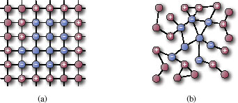
FIGURE 7.1
Graph boundary sets on two different graphs. (a) a 4-adjacency grid graph. (b) an arbitrary undirected graph. Blue vertices correspond to $\mathcal{A}$. Vertices marked by the “?” sign correspond to the internal boundary ${\partial }^{-}\mathcal{A}$ and those marked by the “+” sign correspond to the external boundary ${\partial }^{+}\mathcal{A}$.

7.2.5    p-Laplace Operators

Let p ∈ (0, +∞) be a real number. We introduce the isotropic and anisotropic p-Laplace operators as well as the associated p-Laplacian matrix.

7.2.5.1    p-Laplace Isotropic Operator

The weighted p-Laplace isotropic operator of a function $f\in \mathscr{H}\left(\mathcal{V}\right)$, noted ${\text{Δ}}_{w,p}^i:\mathscr{H}\left(\mathcal{V}\right)\to \mathscr{H}\left(\mathcal{V}\right)$, is defined by:

$\left({\text{Δ}}_{w,p}^{i}f\right)\left({\upsilon }_i\right)=\frac{1}{2}{d}_w^{\ast }\left({\Vert \left({\nabla }_{w}f\right)\left(v_i\right)\Vert }_2^{p-2}\left(d_{w}f\right)\left({\upsilon }_i,{\upsilon }_j\right)\right).$

(7.7)

The isotropic p-Laplace operator of $f\in \mathscr{H}\left(\mathcal{V}\right)$, at a vertex ${\upsilon }_i\in \mathcal{V}$, can be computed by [18, 19, 20, 3]:

$\left({\text{Δ}}_{w,p}^{i}f\right)\left({\upsilon }_i\right)=\frac{1}{2}{\displaystyle \sum _{{\upsilon }_j\sim {\upsilon }_i}\left({\gamma }_{w,p}^{i}f\right)\left({\upsilon }_i,{\upsilon }_j\right)\left(f\left({\upsilon }_i\right)-f\left({\upsilon }_j\right)\right)},$

(7.8)

with

$\left({\gamma }_{w,p}^{i}f\right)\left({\upsilon }_i,{\upsilon }_j\right)=w_{ij}\left({\Vert \left({\nabla }_{w}f\right)\left(v_j\right)\Vert }_2^{p-2}+{\Vert \left({\nabla }_{w}f\right)\left(v_i\right)\Vert }_2^{p-2}\right).$

(7.9)

Proof From (7.7), (7.3) and (7.1), we have:

$\begin{array}{ll}\left({\text{Δ}}_{w,p}^{i}f\right)\left({\upsilon }_i\right)\hfill & =\frac{1}{2}{\displaystyle \sum _{{\upsilon }_j\sim {\upsilon }_i}\sqrt{w_{ij}}}\left(\frac{\left(d_{w}f\right)\left({\upsilon }_j,{\upsilon }_i\right)}{{\Vert \left({\nabla }_{w}f\right)\left(v_j\right)\Vert }^{2-p}}-\frac{\left(d_{w}f\right)\left({\upsilon }_i,{\upsilon }_j\right)}{{\Vert \left({\nabla }_{w}f\right)\left(v_i\right)\Vert }^{2-p}}\right)\hfill \\ \hfill & =\frac{1}{2}{\displaystyle \sum _{{\upsilon }_j\sim {\upsilon }_i}{w}_{ij}}\left(\frac{f\left({\upsilon }_i\right)-f\left({\upsilon }_j\right)}{{\Vert \left({\nabla }_{w}f\right)\left(v_j\right)\Vert }^{2-p}}-\frac{f\left({\upsilon }_j\right)-f\left({\upsilon }_i\right)}{{\Vert \left({\nabla }_{w}f\right)\left(v_i\right)\Vert }^{2-p}}\right).\hfill \end{array}$

(7.10)

This last term is exactly (7.8).

■

The p-Laplace isotropic operator is nonlinear, with the exception of p = 2 (see [18, 19, 20, 3]). In this latter case, it corresponds to the combinatorial graph Laplacian, which is one of the classical second order operators defined in the context of spectral graph theory [25]. Another particular case of the p-Laplace isotropic operator is obtained with p = 1. In this case, it is the weighted curvature of the function f on the graph. To avoid zero denominator in (7.8) when $p\le 1,{\Vert \left({\nabla }_{w}f\right)\left(v_i\right)\Vert }_2$ is replaced by ${\Vert \left({\nabla }_{w}f\right)\left(v_i\right)\Vert }_{2,ϵ}=\sqrt{{\displaystyle \sum _{{\upsilon }_j\sim {\upsilon }_i}{w}_{ij}}{\left(f\left({\upsilon }_j\right)-f\left({\upsilon }_i\right)\right)}^2+{ϵ}^2}$, where ϵ → 0 small fixed constant.

7.2.5.2    p-Laplace Anisotropic Operator

The weighted p-Laplace anisotropic operator of a function $f\in \mathscr{H}\left(\mathcal{V}\right)$, noted ${\text{Δ}}_{w,p}^a:\mathscr{H}\left(\mathcal{V}\right)\to \mathscr{H}\left(\mathcal{V}\right)$, is defined by:

$\left({\text{Δ}}_{w,p}^{a}f\right)\left({\upsilon }_i\right)=\frac{1}{2}{d}_w^{\ast }\left({\left|\left(d_{w}f\right)\left({\upsilon }_i,{\upsilon }_j\right)\right|}^{p-2}\left(d_{w}f\right)\left({\upsilon }_i,{\upsilon }_j\right)\right).$

(7.11)

The anisotropic p-Laplace operator of $f\in \mathscr{H}\left(\mathcal{V}\right)$, at a vertex ${\upsilon }_i\in \mathcal{V}$, can be computed by [26]:

$\left({\text{Δ}}_{w,p}^{a}f\right)\left({\upsilon }_i\right)={\displaystyle \sum _{{\upsilon }_j\sim {\upsilon }_i}\left({\gamma }_{w,p}^{a}f\right)\left({\upsilon }_i,{\upsilon }_j\right)\left(f\left({\upsilon }_i\right)-f\left({\upsilon }_j\right)\right)}.$

(7.12)

with

$\left({\gamma }_{w,p}^{a}f\right)\left({\upsilon }_i,{\upsilon }_j\right)=w_{ij}^{p/2}{\left|f\left({\upsilon }_i\right)-f\left({\upsilon }_j\right)\right|}^{p-2}.$

(7.13)

Proof From (7.11), (7.3) and (7.1), we have

$\begin{array}{r}\hfill \left({\text{Δ}}_{w,p}^{a}f\right)\left({\upsilon }_i\right)=\frac{1}{2}{\displaystyle \sum _{{\upsilon }_j\sim {\upsilon }_i}\sqrt{w_{ij}}}\left(\frac{\left(d_{w}f\right)\left({\upsilon }_j,{\upsilon }_i\right)}{{\left|\left(d_{w}f\right)\left({\upsilon }_i,{\upsilon }_j\right)\right|}^{2-p}}-\frac{\left(d_{w}f\right)\left({\upsilon }_i,{\upsilon }_j\right)}{{\left|\left(d_{w}f\right)\left({\upsilon }_i,{\upsilon }_j\right)\right|}^{2-p}}\right)=\\ \hfill {\displaystyle \sum _{{\upsilon }_j\sim {\upsilon }_i}\sqrt{w_{ij}}}\left(\frac{\left(d_{w}f\right)\left({\upsilon }_j,{\upsilon }_i\right)}{{\left|\left(d_{w}f\right)\left({\upsilon }_i,{\upsilon }_j\right)\right|}^{2-p}}\right)={\displaystyle \sum _{{\upsilon }_j\sim {\upsilon }_i}{w}_{ij}^{\frac{p}{2}}{\left|f\left({\upsilon }_i\right)-f\left({\upsilon }_j\right)\right|}^{p-2}\left(f\left({\upsilon }_i\right)-f\left({\upsilon }_j\right)\right).}\end{array}$

(7.14)

■

This operator is nonlinear if p ≠ 2. In this latter case, it corresponds to the combinatorial graph Laplacian, as the isotropic 2-Laplacian. To avoid zero denominator in (7.12) when p ≤ 1, |f(υ_i) – f(υ_j)| is replaced by |f(υ_i) – f(υ_j)|_ϵ = |f(υ_i) – f(υ_j)| + ϵ, where ϵ → 0 is a small fixed constant.

7.2.6    p-Laplacian Matrix

Finally, the (isotropic or anisotropic) p-Laplacian matrix $L_p^{\ast }$ satisfies the following properties.

(1)  its expression is:

$L_p^{\ast }\left({\upsilon }_i,{\upsilon }_j\right)=\{\begin{array}{ll}\frac{\alpha }{2}{\displaystyle \sum _{{\upsilon }_k\sim {\upsilon }_i}\left({\gamma }_{w,p}^{\ast }f\right)\left({\upsilon }_i,{\upsilon }_k\right)}\hfill & \text{if}{\upsilon }_i={\upsilon }_j\hfill \\ \hfill -\frac{\alpha }{2}\left({\gamma }_{w,p}^{\ast }f\right)\left({\upsilon }_i,{\upsilon }_j\right)& \text{if}{\upsilon }_i\ne {\upsilon }_j\text{and}\left({\upsilon }_i,{\upsilon }_j\right)\in ℰ\hfill \\ \hfill 0& \text{if}\left({\upsilon }_i,{\upsilon }_j\right)\notin ℰ\hfill \end{array}$

(7.15)

with ${\gamma }_{w,p}^{\ast }={\gamma }_{w,p}^i$ and α = 1 for the isotropic case or ${\gamma }_{w,p}^{\ast }={\gamma }_{w,p}^a$ and α = 2 for the anisotropic case.

(2)  For every vector $f\left(u\right),f{\left(u\right)}^{\mathcal{T}}{L}_p^{\ast }f\left(u\right)=\left({\text{Δ}}_{w,p}^{\ast }f\right)\left(u\right)$ with ${\text{Δ}}_{w,p}^{\ast }={\text{Δ}}_{w,p}^i$ or ${\text{Δ}}_{w,p}^{\ast }={\text{Δ}}_{w,p}^a$.

(3)  $L_p^{\ast }$ is symmetric and positive semi-definite (see section 7.4 for a justification).

(4)  $L_p^{\ast }$ has non-negative, real-valued eigenvalues: 0 = s₁ ≤ s₂ ≤ ⋯ ≤ s_N.

Therefore, the (isotropic or anisotropic) p-Laplacian matrix can be used for manifold learning and generalizes approaches based on the 2-Laplacian [27]. New dimensionality reduction methods can be obtained with an eigen-decomposition of the matrix $L_p^{\ast }$. This has been recently explored in [28] with the isotropic p-Laplace operator and in [29] with the anisotropic p-Laplace operator for spectral clustering where a variational algorithm is proposed for generalized spectral clustering.

7.3    Construction of Weighted Graphs

Any discrete domain can be modeled by a weighted graph where each data point is represented by a vertex ${\upsilon }_i\in \mathcal{V}$. This domain can represent unorganized or organized data where functions defined on $\mathcal{V}$ correspond to the data to process. We provide details on defining the graph topology and the graph weights.

7.3.1    Graph Topology

7.3.1.1    Unorganized Data

In this general case, an unorganized set of points $\mathcal{V}\subset {ℝ}^n$ can be seen as a function $f^0:\mathcal{V}\to {ℝ}^m$. Then, defining the set of edges consists in modeling the neighborhood of each vertex based on similarity relationships between feature vectors of the data set. This similarity depends on a pairwise distance measure $\mu :\mathcal{V}\times \mathcal{V}\to {ℝ}^{+}$. A typical choice of μ for unorganized data is the Euclidean distance. Graph construction is application dependent, and no general rules can be given. However, there exists several methods to construct a neighborhood graph. The interested reader can refer to [30] for a survey on proximity and neighborhood graphs. We focus on two classes of graphs: a modified version of k-nearest neighbors graphs and τ-neighborhood graphs.

The τ-neighborhood graph, noted ${\mathcal{G}}_{\tau }$ is a weighted graph where the τ-neighborhood ${\mathcal{N}}_{\tau }$ for a vertex υ_i is defined as ${\mathcal{N}}_{\tau }\left({\upsilon }_i\right)=\left\{{\upsilon }_j\in \mathcal{V}\left\{{\upsilon }_i\right\}:\mu \left({\upsilon }_i,{\upsilon }_j\right)\le \tau \right\}$ where τ > 0 is a threshold parameter.

The k-nearest neighbors graph, noted k-NNG_τ is a weighted graph where each vertex υ_i is connected to its k nearest neighbors that have the smallest distance measure towards υ_i according to function μ in ${\mathcal{N}}_{\tau }$. Since this graph is directed, a modified version is used to make it undirected i.e., $ℰ=\left\{\left({\upsilon }_i,{\upsilon }_j\right):{\upsilon }_i\in {\mathcal{N}}_{\tau }\left({\upsilon }_j\right)\text{or}{\upsilon }_j\in {\mathcal{N}}_{\tau }\left({\upsilon }_i\right)\right\}$ for ${\upsilon }_i,{\upsilon }_j\in \mathcal{V}$. When τ = ∞, one obtains the k-NNG_∞ where the k nearest neighbors are computed for all the set $\mathcal{V}\left\{{\upsilon }_i\right\}$. For the sake of clarity, the k-NNG_∞ will be noted k-NNG.

7.3.1.2    Organized Data

Typical cases of organized data are signals, gray-scale, or color images (eventually in 2D or 3D). Such data can be seen as functions $f^0:\mathcal{V}\subset {\mathbb{Z}}^n\to {ℝ}^m$. Then, the distance μ used to construct the graph corresponds to a distance between spatial coordinates associated to vertices. Several distances can be considered. Among those, for a 2D image, we can quote the city-block distance: $\mu \left({\upsilon }_i,{\upsilon }_j\right)=\left|x_i^1-x_j^1\right|+\left|x_i^2-x_j^2\right|$ or the Chebyshev distance: $\mu \left({\upsilon }_i,{\upsilon }_j\right)=\max \left(\left|x_i^1-x_j^1\right|,\left|x_i^2-x_j^2\right|\right)$ where a vertex υ_i is associated with its ${\left(x_i^1,x_i^2\right)}^{\mathcal{T}}$ spatial coordinates. With these distances and a τ-neighborhood graph, the usual adjacency graphs used in 2D image processing are obtained where each vertex corresponds to an image pixel. Then, a 4-adjacency and an 8-adjacency grid graph (denoted ${\mathcal{G}}_0$ and ${\mathcal{G}}_1$, respectively) can be obtained with the city-block and the Chebyshev distance, respectively (with τ ≤ 1). More generally, ((2s + 1)² − 1)-adjacency graphs are obtained with a Chebyshev distance with τ ≤ s and s ≥ 1. This corresponds to adding edges between the central pixel and the other pixels within a square window of size (2s + 1)². Similar remarks apply for the construction of graphs on 3D images where vertices are associated to voxels.

The region adjacency graphs (RAGs) can also be considered for image processing. Each vertex of this graph corresponds to one region. The set of edges is obtained with an adjacency distance: μ(υ_i, υ_j) = 1 if υ_i and υ_j are adjacent and μ(υ_i, υ_j) = ∞, otherwise, together with a τ-neighborhood graph (τ = 1): this corresponds to the Delaunay graph of an image partition.

Finally, we can mention the cases of polygonal curves or surfaces that have natural graph representations where vertices correspond to mesh vertices and edges are mesh edges.

7.3.2    Graph Weights

For an initial function $f^0:\mathcal{V}\to {ℝ}^m$, a similarity relationship between data can be incorporated within edge weights according to a measure of similarity $g:ℰ\to \left[0,1\right]$ with $w\left(e_{ij}\right)=g\left(e_{ij}\right),\forall e_{ij}\in ℰ$. Computing distances between vertices consists in comparing their features, generally depending on f⁰. To this end, each vertex υ_i is associated with a feature vector $F_{\tau }^{f^0}:\mathcal{V}\to {ℝ}^{m\times q}$ where q corresponds to this vector size:

$F_{\tau }^{f^0}\left({\upsilon }_i\right)={\left(f^0\left({\upsilon }_j\right):{\upsilon }_j\in {\mathcal{N}}_{\tau }\left({\upsilon }_i\right)\cup \left\{{\upsilon }_i\right\}\right)}^{\mathcal{T}}.$

(7.16)

Then, the following weight functions can be considered. For an edge e_ij and a distance measure $\rho :{ℝ}^{m\times q}\times {ℝ}^{m\times q}\to ℝ$ associated to $F_{\tau }^{f^0}$, we can have:

$\begin{array}{l}{g}_1\left(e_{ij}\right)=1\left(\text{unweighted}\text{case}\right),\hfill \\ g_2\left(e_{ij}\right)=\exp \left(-\rho {\left(F_{\tau }^{f^0}\left({\upsilon }_i\right),F_{\tau }^{f^0}\left({\upsilon }_j\right)\right)}^2/{\sigma }^2\right)\text{with}\sigma >0,\hfill \\ g_3\left(e_{ij}\right)=1/\left(1+\rho \left(F_{\tau }^{f^0}\left({\upsilon }_i\right),F_{\tau }^{f^0}\left({\upsilon }_j\right)\right)\right)\hfill \end{array}$

(7.17)

Usually, ρ is the Euclidean distance function. Several choices can be considered for the expression of $F_{\tau }^{f^0}$ depending on the features to preserve. The simplest one is $F_0^{f^0}=f^0$.

In image processing, an important feature vector $F_{\tau }^{f^0}$ is provided by image patches. For a gray-scale image $f^0:\mathcal{V}\to ℝ$, the vector $F_{\tau }^{f^0}$ defined by an image patch corresponds to the values of f⁰ in a square window of size (2τ + 1)² centered at a vertex (a pixel). Figure 7.2(a) shows examples of image patches. A given vertex (central pixel represented in red) is not only characterized by its gray-scale value but also by the gray-scale values contained in a square window (a patch) centered on it. Figure 7.2(b) shows the difference between local and nonlocal interaction in a 8-adjacency grid graph by adding nonlocal edges between vertices not spatially connected but close in a 5 × 5 neighborhood. This feature vector has been proposed for texture synthesis [31], and recently used for image restoration and filtering [32, 33]. In image processing, such configurations are called “nonlocal”, and these latter works have shown the efficiency of nonlocal patch-based methods as compared to local ones, in particular, by better capturing complex structures such as objects boundaries or fine and repetitive patterns. The notion of “nonlocality” (as defined by [32]) includes two notions: (1) the search window of the most similar neighbors for a given pixel and (2) the feature vector to compare these neighbors. In [32], nonlocal processing consists in comparing, for a given pixel, all the patches contained in an image. In practice, to avoid this high computational cost, one can use a search window of fixed size. Local and nonlocal methods are naturally included in weighted graphs. Indeed, nonlocal patch-based configurations are simply expressed by the graph topology (the vertex neighborhood) and the edge weights (distances between vertex features). Nonlocal processing of images becomes local processing on similarity graphs. Our operators on graphs (weighted differences and gradients) naturally enable local and nonlocal configurations (with the weight function and the graph topology) and introduce new adaptive tools for image processing.

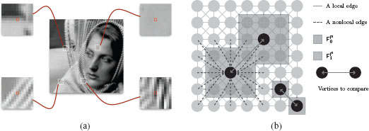
FIGURE 7.2
(a) Four examples of image patches. Central pixels (in red) are associated with vectors of gray-scale values within a patch of size 13 × 13 $\left(F_6^{f^0}\right)$. (b) Graph topology and feature vector illustration: a 8-adjacency grid graphs is constructed. The vertex surrounded by a red box shows the use of the simplest feature vector, i.e., the initial function. The vertex surrounded by a green box shows the use of a feature vector that exploits patches.

7.4    p-Laplacian Regularization on Graphs

Let $f^0:\mathcal{V}\to ℝ$ be a given function defined on the vertices of a weighted graph $\mathcal{G}=\left(\mathcal{V},ℰ,w\right)$. In a given context, the function f⁰ represents an observation of a clean function $g:\mathcal{V}\to ℝ$ corrupted by a given noise n such that f⁰ = g + n. Such noise is assumed to have zero mean and variance σ², which usually corresponds to observation errors. To recover the uncorrupted function g, a commonly used method is to seek for a function $f:\mathcal{V}\to ℝ$ which is regular enough on $\mathcal{G}$, and also close enough to f⁰. This inverse problem can be formalized by the minimization of an energy functional, which typically involves a regularization term plus an approximation term (also called fitting term). We consider the following variational problem [18, 19, 20, 3]:

$g\approx \underset{f:\mathcal{V}\to ℝ}{\min }\left\{{ℰ}_{w,p}^{\ast }\left(f,f^0,\lambda \right)=R_{w,p}^{\ast }\left(f\right)+\frac{\lambda }{2}{\Vert f-f^0\Vert }_2^2\right\},$

(7.18)

where the regularization functional $R_{w,p}^{\ast }:\mathscr{H}\left(\mathcal{V}\right)\to ℝ$ can correspond to an isotropic $R_{w,p}^i$ or an anisotropic $R_{w,p}^a$ functionnal. The isotropic regularization functionnal $R_{w,p}^i$ is defined by the ${ℒ}_2$ norm of the gradient and is the discrete p-Dirichlet form of the function $f\in \mathscr{H}\left(\mathcal{V}\right)$:

$\begin{array}{ll}{R}_{w,p}^i\left(f\right)\hfill & =\frac{1}{p}{\displaystyle \sum _{{\upsilon }_i\in \mathcal{V}}{\Vert \left({\nabla }_{w}f\right)\left(v_i\right)\Vert }_2^p}=\frac{1}{p}{\langle f,{\text{Δ}}_{w,p}^{i}f\rangle }_{\mathscr{H}\left(\mathcal{V}\right)}\hfill \\ \hfill & =\frac{1}{p}{\displaystyle \sum _{{\upsilon }_i\in \mathcal{V}}{\left[{\displaystyle \sum _{{\upsilon }_j\sim {\upsilon }_i}\left[w_{ij}{\left(f\left({\upsilon }_j\right)-f\left({\upsilon }_i\right)\right)}^2\right]}\right]}^{\frac{p}{2}}.}\hfill \end{array}$

(7.19)

The anisotropic regularization functionnal $R_{w,p}^a$ is defined by the ${ℒ}_p$ norm of the gradient:

$\begin{array}{ll}{R}_{w,p}^a\left(f\right)\hfill & =\frac{1}{p}{\displaystyle \sum _{{\upsilon }_i\in \mathcal{V}}{\Vert \left({\nabla }_{w}f\right)\left(v_i\right)\Vert }_p^p}=\frac{1}{p}{\langle f,{\text{Δ}}_{w,p}^{a}f\rangle }_{\mathscr{H}\left(\mathcal{V}\right)}\hfill \\ \hfill & =\frac{1}{p}{\displaystyle \sum _{{\upsilon }_i\in \mathcal{V}}{\displaystyle \sum _{{\upsilon }_j\sim {\upsilon }_i}\left[w_{ij}^{p/2}{\left|f\left({\upsilon }_j\right)-f\left({\upsilon }_i\right)\right|}^p\right]}.}\hfill \end{array}$

(7.20)

Both the previous regularization functionals show the fact that ${\text{Δ}}_{w,p}^i$ and ${\text{Δ}}_{w,p}^a$ are positive semi-definite (since $R_{w,p}^i\ge 0$ and $R_{w,p}^a\ge 0$). The isotropic and anisotropic versions of ${ℰ}_{w,p}^{\ast }$ are, respectively, denoted by ${ℰ}_{w,p}^i$ and ${ℰ}_{w,p}^a$. The trade-off between the two competing terms in the functional ${ℰ}_{w,p}^{\ast }$ is specified by the fidelity parameter λ ≥ 0. By varying the value of λ, the variational problem (7.18) allows to describe the function f⁰ at different scales, each scale corresponding to a value of λ. The degree of regularity, which has to be preserved, is controlled by the value of p > 0.

7.4.1    Isotropic Diffusion Processes

First, we consider the case of an isotropic regularization functional, i.e., $R_{w,p}^{\ast }=R_{w,p}^i$. When p ≥ 1, the energy ${ℰ}_{w,p}^i$ is a convex functional of functions of $\mathscr{H}\left(\mathcal{V}\right)$. To get the solution of the minimizer (7.18), we consider the following system of equations

$\frac{\partial {ℰ}_{w,p}^i\left(f,f^0,\lambda \right)}{\partial f\left({\upsilon }_i\right)}=0,\forall {\upsilon }_i\in \mathcal{V},$

(7.21)

which is rewritten as:

$\frac{\partial R_{w,p}^i\left(f\right)}{\partial f\left({\upsilon }_i\right)}+\lambda \left(f\left({\upsilon }_i\right)-f^0\left({\upsilon }_i\right)\right)=0,\forall {\upsilon }_i\in \mathcal{V}.$

(7.22)

The solution of the latter system is computed by using the following property. Let f be a function in $\mathscr{H}\left(\mathcal{V}\right)$, one can prove from (7.19) that [3],

$\frac{\partial R_{w,p}^i\left(f\right)}{\partial f\left({\upsilon }_i\right)}=2\left({\text{Δ}}_{w,p}^{i}f\right)\left({\upsilon }_i\right).$

(7.23)

Proof Let υ₁ be a vertex of $\mathcal{V}$. From (7.19), the υ₁-th term of the derivative of $R_{w,p}^i\left(f\right)$ is given by:

$\frac{\partial R_{w,p}^i\left(f\right)}{\partial f\left({\upsilon }_1\right)}=\frac{1}{p}\frac{\partial }{\partial f\left({\upsilon }_1\right)}\left({\displaystyle \sum _{{\upsilon }_i\in \mathcal{V}}{\left({\displaystyle \sum _{{\upsilon }_j\sim {\upsilon }_i}{w}_{ij}{\left(f\left({\upsilon }_j\right)-f\left({\upsilon }_i\right)\right)}^2}\right)}^{\frac{p}{2}}}\right).$

(7.24)

It only depends on the edges incident to υ₁. Let υ_l, …, υ_k be the vertices of $\mathcal{V}$ connected to υ₁ by an edge of $ℰ$. Then, by using the chain rule, we have:

$\begin{array}{ll}\frac{\partial R_{w,p}^i\left(f\right)}{\partial f\left({\upsilon }_1\right)}\hfill & =-{\displaystyle \sum _{{\upsilon }_j\sim {\upsilon }_1}{w}_{1j}\left(f\left({\upsilon }_j\right)-f\left({\upsilon }_1\right)\right){\Vert \left({\nabla }_{w}f\right)\left(v_1\right)\Vert }_2^{p-2}}\hfill \\ \hfill & +w_{l1}\left(f\left({\upsilon }_1\right)-f\left({\upsilon }_l\right)\right){\Vert \left({\nabla }_{w}f\right)\left(v_l\right)\Vert }_2^{p-2}\hfill \\ \hfill & +\dots +w_{k1}\left(f\left({\upsilon }_1\right)-f\left({\upsilon }_k\right)\right){\Vert \left({\nabla }_{w}f\right)\left(v_k\right)\Vert }_2^{p-2},\hfill \end{array}$

(7.25)

which is equal to: ${\displaystyle {\sum }_{{\upsilon }_j\sim {\upsilon }_1}{w}_{1j}\left(f\left({\upsilon }_1\right)-f\left({\upsilon }_j\right)\right)\left({\Vert \left({\nabla }_{w}f\right)\left(v_1\right)\Vert }_2^{p-2}+{\Vert \left({\nabla }_{w}f\right)\left(v_j\right)\Vert }_2^{p-2}\right)}$. From (7.8), this latter expression is exactly $2{\text{Δ}}_{w,p}^{i}f\left({\upsilon }_1\right)$.

■

The system of equations is then rewritten as

$2\left({\text{Δ}}_{w,p}^{i}f\right)\left({\upsilon }_i\right)+\lambda \left(f\left({\upsilon }_i\right)-f^0\left({\upsilon }_i\right)\right)=0,\forall {\upsilon }_i\in \mathcal{V},$

(7.26)

which is equivalent to the following system of equations:

$\left(\lambda +{\displaystyle \sum _{{\upsilon }_j\sim {\upsilon }_i}\left({\gamma }_{w,p}^{i}f\right)\left({\upsilon }_i,{\upsilon }_j\right)}\right)f\left({\upsilon }_i\right)-{\displaystyle \sum _{{\upsilon }_j\sim {\upsilon }_i}\left({\gamma }_{w,p}^{i}f\right)\left({\upsilon }_i,{\upsilon }_j\right)}f\left({\upsilon }_j\right)=\lambda f^0\left({\upsilon }_i\right).$

(7.27)

We use the linearized Gauss-Jacobi iterative method to solve the previous system. Let n be an iteration step, and let f⁽ⁿ⁾ be the solution at the step n. Then, the method is given by the following algorithm:

$\{\begin{array}{ll}\hfill f^{\left(0\right)}& =f^0\hfill \\ f^{\left(n+1\right)}\left({\upsilon }_i\right)\hfill & =\frac{\lambda f^0\left({\upsilon }_i\right)+{\displaystyle {\sum }_{{\upsilon }_j\sim {\upsilon }_i}\left({\gamma }_{w,p}^i{f}^{\left(n\right)}\right)\left({\upsilon }_i,{\upsilon }_j\right)}{f}^{\left(n\right)}\left({\upsilon }_j\right)}{\lambda +{\displaystyle {\sum }_{{\upsilon }_j\sim {\upsilon }_i}\left({\gamma }_{w,p}^i{f}^{\left(n\right)}\right)\left({\upsilon }_i,{\upsilon }_j\right)}},\forall {\upsilon }_i\in \mathcal{V}.\hfill \end{array}$

(7.28)

with ${\gamma }_{w,p}^i$ as defined in (7.9). We present in this chapter only this simple method of resolution, but more efficient methods should be preferred [34, 35].

7.4.2    Anisotropic Diffusion Processes

Second, we consider the case of an anisotropic regularization functional, i.e., $R_{w,p}^{\ast }=R_{w,p}^a$. When p ≥ 1, the energy ${ℰ}_{w,p}^a$ is a convex functional of functions of $\mathscr{H}\left(\mathcal{V}\right)$. We can follow the same resolution as for the isotropic case. Indeed, to get the solution of the minimizer (7.18), we consider the following system of equations:

$\frac{\partial R_{w,p}^a\left(f\right)}{\partial f\left({\upsilon }_i\right)}+\lambda \left(f\left({\upsilon }_i\right)-f^0\left({\upsilon }_i\right)\right)=0,\forall {\upsilon }_i\in \mathcal{V}.$

(7.29)

One can also prove from (7.20), using the chain rule similarly than for the isotropic case, that [26]

$\frac{\partial R_{w,p}^a\left(f\right)}{\partial f\left({\upsilon }_i\right)}=\left({\text{Δ}}_{w,p}^{a}f\right)\left({\upsilon }_i\right).$

(7.30)

The previous system of equations is rewritten as

$\left({\text{Δ}}_{w,p}^{a}f\right)\left({\upsilon }_i\right)+\lambda \left(f\left({\upsilon }_i\right)-f^0\left({\upsilon }_i\right)\right)=0,\forall {\upsilon }_i\in \mathcal{V}.$

(7.31)

Similarly as for the isotropic case, we use the linearized Gauss-Jacobi iterative method to solve the previous system. Let n be an iteration step, and let f⁽ⁿ⁾ be the solution at the step n. Then, the method is given by the following algorithm:

$\{\begin{array}{ll}\hfill f^{\left(0\right)}& =f^0\hfill \\ f^{\left(n+1\right)}\left({\upsilon }_i\right)\hfill & =\frac{\lambda f^0\left({\upsilon }_i\right)+{\displaystyle {\sum }_{{\upsilon }_j\sim {\upsilon }_i}\left({\gamma }_{w,p}^a{f}^{\left(n\right)}\right)\left({\upsilon }_i,{\upsilon }_j\right)f^{\left(n\right)}\left({\upsilon }_j\right)}}{\lambda +{\displaystyle {\sum }_{{\upsilon }_j\sim {\upsilon }_i}\left({\gamma }_{w,p}^a{f}^{\left(n\right)}\right)\left({\upsilon }_i,{\upsilon }_j\right)}},\forall {\upsilon }_i\in \mathcal{V}.\hfill \end{array}$

(7.32)

${\gamma }_{w,p}^a$ as defined in (7.13).

7.4.3    Related Works

The two regularization methods describe a family of discrete isotropic or anisotropic diffusion processes [3, 26], which are parameterized by the structure of the graph (topology and weight function), the parameter p, and the parameter λ. At each iteration of the algorithm (7.28), the new value f⁽ⁿ⁺¹⁾(υ_i) depends on two quantities: the original value f⁰(υ_i), and a weighted average of the filtered values of f⁽ⁿ⁾ in a neighborhood of υ_i. The familly of induced filters exhibits strong links with numerous existing filters for image filtering and extends them to the processing of data of arbitrary dimensions on graphs (see [3, 26]). Links with spectral methods can also be exhibited.

7.4.3.1    Related Works in Image Processing

When p = 2, both the isotropic and anisotropic p-Laplacian are the classical combinatorial Laplacian. With λ = 0, the solution of the diffusion processes is the solution of the heat equation Δ_wf(υ_i) = 0, for all ${\upsilon }_i\in \mathcal{V}$. Moreover, since it is also the solution of the minimization of the Dirichlet energy $R_{w,2}^{\ast }\left(f\right)$, the diffusion performs also Laplacian smoothing. Many other specific filters are related to the diffusion processes we propose (see [3, 26] for details). In particular, with specific values of p, λ, graph topologies, and weights, it is easy to recover Gaussian filtering, bilateral filtering [36], the TV digital filter [37], median and minimax filtering [10] but also the NLMeans [32]. The p-Laplacian regularization we propose can as well be considered as the discrete analogue of the recently proposed continuous nonlocal anisotropic functionals [33, 38, 39]. Finally, our framework based on the isotropic or anisotropic p-Laplacian generalizes all these approaches and extends them to weighted graphs of the arbitrary topologies.

7.4.3.2    Links with Spectral Methods

When λ = 0 and p = 2, an iteration of the diffusion process given by $f^{\left(n+1\right)}\left({\upsilon }_i\right)={\displaystyle {\sum }_{{\upsilon }_j\sim {\upsilon }_i}{\text{Φ}}_{ij}\left(f^{\left(n\right)}\right)f^{\left(n\right)}\left({\upsilon }_j\right)}$, $\forall {\upsilon }_i\in \mathcal{V}$ with

${\text{Φ}}_{ij}\left(f\right)=\frac{\left({\gamma }_{w,p}^{\ast }f\right)\left({\upsilon }_i,{\upsilon }_j\right)f\left({\upsilon }_j\right)}{{\displaystyle {\sum }_{{\upsilon }_j\sim {\upsilon }_i}\left({\gamma }_{w,p}^{\ast }f\right)\left({\upsilon }_i,{\upsilon }_j\right)}},\forall \left({\upsilon }_i,{\upsilon }_j\right)\in ℰ.$

(7.33)

For the isotropic case, ${\gamma }_{w,p}^{\ast }f={\gamma }_{w,p}^{i}f$ and for the anisotropic case, ${\gamma }_{w,p}^{\ast }f={\gamma }_{w,p}^{a}f$. Let Q be the Markov matrix defined by

$\{\begin{array}{ll}Q\left({\upsilon }_i,{\upsilon }_j\right)=\hfill & {\text{Φ}}_{ij}\text{if}\left({\upsilon }_i,{\upsilon }_j\right)\in ℰ\hfill \\ Q\left({\upsilon }_i,{\upsilon }_j\right)=\hfill & \hfill 0\text{if}\left({\upsilon }_i,{\upsilon }_j\right)\notin ℰ.\end{array}$

(7.34)

Then, an iteration of the diffusion process (7.28) with λ = 0 can be written in matrix form as f⁽ⁿ⁺¹⁾ = Qf⁽ⁿ⁾ = Q⁽ⁿ⁾f⁰, where Q is a stochastic matrix (nonnegative, symmetric, unit row sum). An equivalent way to look at the power of Q in the diffusion process is to decompose each value of f on the first eigenvectors of Q, therefore the diffusion process can be interpreted as a filtering in the spectral domain [40].

Moreover, it is also shown in [29] that one can obtain the eigenvalues and eigenvectors of the p-Laplacian by computing the global minima and minimizers of the functional $F_{w,p}^{\ast }\left(f\right)=\frac{R_{w,p}^{\ast }\left(f\right)}{{\Vert f\Vert }_p^p}$ according to the generalized Rayleigh-Ritz principle. This states that if $F_{w,p}^{\ast }$ has critical point at $\phi \in {ℝ}^{\left|\mathcal{V}\right|}$, then φ is a p-eigenvector of ${\text{Δ}}_{w,p}^{\ast }$ and the eigenvalue s is then $s=F_{w,p}^{\ast }\left(\phi \right)$. This provides a variational interpretation of the p-Laplacian spectrum and shows that the eigenvectors of the p-Laplacian can be obtained directly in the spatial domain. Therefore, when λ = 0, the proposed diffusion process is linked to a spectral analysis of f.

7.4.4    Interpolation of Missing Data on Graphs

Many tasks in image processing and computer vision can be formulated as interpolation problems. Interpolating data consists in constructing new values for missing data in coherence with a set of known data. We consider that data are defined on a general domain represented on a graph $\mathcal{G}=\left(\mathcal{V},ℰ,w\right)$. Let $f^0:{\mathcal{V}}_0\to ℝ$ be a function with ${\mathcal{V}}_0\subset \mathcal{V}$ be the subset of vertices from the whole graph with known values. Consequently, $\mathcal{V}{\mathcal{V}}_0$ corresponds to the vertices with unknown values. The interpolation consists in predicting a function $f:\mathcal{V}\to ℝ$ according to f⁰. This comes to recover values of f for the vertices of $\mathcal{V}{\mathcal{V}}_0$ given values for vertices of ${\mathcal{V}}_0$. Such a problem can be formulated by considering the following regularization problem on the graph:

$\underset{f:\mathcal{V}\to ℝ}{\min }{R}_{w,p}^{\ast }\left(f\right)+\lambda \left({\upsilon }_i\right){\Vert f\left({\upsilon }_i\right)-f^0\left({\upsilon }_i\right)\Vert }_2^2.$

(7.35)

Since f⁰(υ_i) is known only for vertices of ${\mathcal{V}}_0$, the Lagrange parameter is defined as $\lambda :\mathcal{V}\to ℝ$:

$\lambda \left({\upsilon }_i\right)=\{\begin{array}{ll}\lambda \hfill & \text{if}{\upsilon }_i\in {\mathcal{V}}_0\hfill \\ 0\hfill & \text{otherwise}.\hfill \end{array}$

(7.36)

Then, the isotropic (7.28) and anisotropic (7.32) diffusion processes can be directly used to perform the interpolation. In the sequel, we show how we can use our formulation for image clustering, inpainting and colorization.

7.4.4.1    Semi-Supervised Image Clustering

Numerous automatic segmentation schemes have been proposed in the literature, and they have shown their efficiency. Meanwhile, recent interactive image segmentation approaches have been proposed. They reformulate image segmentation into semisupervised approaches by label propagation strategies [41, 42, 43]. The recent power watershed formulation [44] is one of the most recent formulation, that provides a common framework for seeded image segmentation. Other applications of these label diffusion methods can be found in [21, 45]. The interpolation regularization-based functional (7.35) can be naturally adapted to address this learning problem for semisupervised segmentation. We rewrite the problem as [46]: let $\mathcal{V}=\left\{{\upsilon }_1,\dots ,{\upsilon }_N\right\}$ be a finite set of data, where each data υ_i is a vector of ${ℝ}^m$, and let $\mathcal{G}=\left(\mathcal{V},ℰ,w\right)$ be a weighted graph such that data are connected by an edge of $ℰ$. The semi-supervised clustering of $\mathcal{V}$ consists in grouping the set $\mathcal{V}$ into k classes with k, the number of classes (known a priori). The set $\mathcal{V}$ is composed of labeled and unlabeled data. The aim is then to estimate the unlabeled data from labeled ones.

Let ${\mathcal{C}}_l$ be a set of labeled vertices, these latter belonging to the l^th class. Let ${\mathcal{V}}_0={\displaystyle \cup {\left\{{\mathcal{C}}_l\right\}}_{l=1,\dots ,k}}$ be the set of initial labeled vertices, and let $\mathcal{V}{\mathcal{V}}_0$ be the initial unlabeled vertices. Each vertex of ${\upsilon }_i\in \mathcal{V}$ is then described by a vector of labels $f^0\left(v_i\right)={\left(f_l^0\left({\upsilon }_i\right)\right)}_{l=1,\dots ,k}^{\mathcal{T}}$ with

$f_l^0\left({\upsilon }_i\right)=\{\begin{array}{ll}+1\hfill & \text{if}{\upsilon }_i\in {\mathcal{C}}_l\hfill \\ 0\hfill & \text{otherwise}.\hfill \\ 0\hfill & \forall {\upsilon }_i\in \mathcal{V}{\mathcal{V}}_0\hfill \end{array}$

(7.37)

The semi-supervised clustering problem then reduces to interpolate the labels of the unlabeled vertices $\left(\mathcal{V}{\mathcal{V}}_0\right)$ from the labeled ones $\left({\mathcal{V}}_0\right)$. To solve this interpolation problem, we consider the variational problem (7.35). We set λ(υ_i) = +∞ to avoid the modification of the initial labels.

At the end of the label propagation processes, the class membership probabilities can be estimated, and the final classification can be obtained for a given vertex ${\upsilon }_i\in \mathcal{V}$ by the following formulation:

$\text{arg}\underset{l\in 1,\dots ,k}{\text{max}}\left\{\frac{f_l^{\left(t\right)}\left({\upsilon }_i\right)}{{\displaystyle {\sum }_l{f}_l^{\left(t\right)}\left({\upsilon }_i\right)}}\right\}$

(7.38)

7.4.4.2    Geometric and Texture Image Inpainting

The inpainting process consists in filling in the missing parts of an image with the most appropriate data in order to obtain harmonious and hardly detectable reconstructed zones. Recent works on image and video inpainting may fall under two main categories, namely, the geometric algorithms and the exemplar-based ones. The first category employs partial differential equations [47]. The second group of inpainting algorithms is based on the texture synthesis [31]. We can restore the missing data using the interpolation regularization-based functional (7.35) that also enables us to take into account either local and nonlocal information. The main advantage is the unification of the geometric and texture-based techniques [48]. The geometric aspect is taken into account though the graph topology, and the texture aspect is expressed by the graph weights. Therefore, by varying both these geometric and texture aspects, we can recover many approaches proposed so far in literature and extend them to weighted graphs of arbitrary topologies.

Let ${\mathcal{V}}_0\subset \mathcal{V}$ be the subset of the vertices corresponding to the original known parts of the image. The inpainting purpose is to interpolate the known values of f⁰ from ${\mathcal{V}}_0$ to $\mathcal{V}{\mathcal{V}}_0$. Our method consists in filling the inpainting mask from its outer line ${\partial }^{-}{\mathcal{V}}_0$ to its center recursively in a series of nested outlines. Our proposed regularization process (7.35) is applied iteratively on each node ${\upsilon }_i\in {\partial }^{-}{\mathcal{V}}_0$. Since at one iteration, the inpainting is performed only on vertices of ${\partial }^{-}{\mathcal{V}}_0$, the data-term is not used in (7.35). Moreover, we enforce the computed value of a vertex of ${\partial }^{-}{\mathcal{V}}_0$ to not use the estimated values of other vertices of ${\partial }^{-}{\mathcal{V}}_0$ even if they are neighbors. This is needed to reduce the risk of error propagation. Once convergence is reached for the entire outer line ${\partial }^{-}{\mathcal{V}}_0$, this subset of vertices is added to $\mathcal{V}{\mathcal{V}}_0$ and removed from ${\mathcal{V}}_0$. The weights of the graph are also updated accordingly (see [49] for an explicit modeling of the weight update step). The process is iterated until the set ${\mathcal{V}}_0$ is empty.

7.4.4.3    Image Colorization

Colorization is the process of adding color to monochrome images. It is usually made by hand by color experts but this process is tedious and very time-consuming. In recent years, several methods have been proposed for colorization [50, 51] that require less intensive manual efforts. These techniques colorize the image based on the user’s input color scribbles and are mainly based on a diffusion process. However, most of these diffusion processes only use local pixel interactions that cannot properly describe complex structures expressed by nonlocal interactions. As we already discussed, with our formulations, the integration of nonlocal interactions is easy to obtain. We now explain how to perform image colorization with the proposed framework [52]. From a gray level image $f^l:\mathcal{V}\to ℝ$, a user provides an image of color scribbles $f^s:{\mathcal{V}}_s\subset \mathcal{V}\to {ℝ}^3$ that defines a mapping from vertices to a vector of RGB color channels: $f^s\left(v_i\right)={\left[f_1^s\left({\upsilon }_i\right),f_2^s\left({\upsilon }_i\right),f_3^s\left({\upsilon }_i\right)\right]}^{\mathcal{T}}$ where $f_j^s:\mathcal{V}\to ℝ$ is the j-th component of f^s(v_i). From these functions, one computes $f^c:\mathcal{V}\to {ℝ}^3$ that defines a mapping from the vertices to a vector of chrominances:

$\{\begin{array}{l}{f}^c\left(v_i\right)={\left[\frac{f_1^s\left({\upsilon }_i\right)}{f^l\left({\upsilon }_i\right)},\frac{f_2^s\left({\upsilon }_i\right)}{f^l\left({\upsilon }_i\right)},\frac{f_3^s\left({\upsilon }_i\right)}{f^l\left({\upsilon }_i\right)}\right]}^{\mathcal{T}},\forall {\upsilon }_i\in {\mathcal{V}}_s.\hfill \\ f^c\left(v_i\right)={\left[0,0,0\right]}^{\mathcal{T}},\forall {\upsilon }_i\notin {\mathcal{V}}_s.\hfill \end{array}$

(7.39)

We then consider the regularization of f^c(v_i) by using the interpolation regularization-based functional (7.35) with algorithms (7.28) or (7.32). Since the weights of the graph cannot be computed from f^c since it is unknown, $\left({\gamma }_{w,p}^{\ast }{f}^c\right)\left(u,\upsilon \right)$ is replaced by $\left({\gamma }_{w,p}^{\ast }{f}^l\right)\left(u,\upsilon \right)$ and weights are computed on the gray level image f^l. Moreover, the data-term is taken into account only on the initial known vertices of ${\mathcal{V}}_s$ with a small value of λ(υ_i) to enable the modification of the original color scribble to avoid annoying visual effects. At convergence, final colors are obtained by $f^l\left({\upsilon }_i\right)\times {\left[f_1^{c^{\left(t\right)}}\left({\upsilon }_i\right),f_2^{c^{\left(t\right)}}\left({\upsilon }_i\right),f_3^{c^{\left(t\right)}}\left({\upsilon }_i\right)\right]}^{\mathcal{T}}$, $\forall {\upsilon }_i\in \mathcal{V}$ where t is the iteration number.

7.5    Examples

In this section, we illustrate the abilities of p-Laplace (isotropic and anisotropic) regularization on graphs for simplification and interpolation of any function defined on a finite set of discrete data living in ${ℝ}^m$. This is achieved by constructing a weighted graph $\mathcal{G}=\left(\mathcal{V},ℰ,w\right)$ and by considering the function to be simplified as a function $f^0:\mathcal{V}\to {ℝ}^m$, defined on the vertices of $\mathcal{G}$. The simplification processes operate on vector-valued function with one process per vector component. Component-wise processing of vector-valued data can have serious drawbacks and it is preferable to drive the simplification processes by equivalent geometric attributes, taking the coupling between vector components into account. As in [3], this is done by using the same gradient for all components (a vectorial gradient).

7.5.1    Regularization-Based Simplification

We illustrate the abilities of our approach for the simplification of functions representing images or images’ manifold. Several graph topologies are also considered.

Let f⁰ be a color image of N pixels, with $f^0:\mathcal{V}\subset {\mathbb{Z}}^2\to {ℝ}^3$, which defines a mapping from the vertices to color vectors. Figure 7.3 shows sample results obtained with different parameters of the proposed isotropic and anisotropic regularization: different values of p, different values of λ, different weight functions, and different graph topologies. The PSNR value between the filtering result and the original uncorrupted image are also provided. The first row of Figure 7.3 presents the initial image and the original image corrupted by Gaussian noise of variance σ = 15. Below the first row, the first column presents results obtained on a 8-adjacency grid graph (S₁) for isotropic and anistropic filtering with p ∈ {2, 1} and λ = 0.005. These results correspond to the classical results that can be obtained with the digital TV and ${ℒ}_2$ filters of Chan and Osher [7, 37]. When the weights are not constant, our approach extends these previous works and enables the production of better visual results by using computed edge weights as depicted in the second column of Figure 7.3. Moreover, the use of the curvature with p =1 enables a better preservation of edges and fine structures with a small advantage for the isotropic regularization. Finally, all these advantages of our approach are further stressed once a nonlocal configuration is used. This enhances once again the preservation of edges and the production of flat zones. These results are presented in the last column of Figure 7.3 on a 80-adjancency graph $\left({\mathcal{G}}_4\right)$ with 5 × 5 patches as feature vectors. This shows how our proposed framework generalizes the NLMeans filter [32].

To further illustrate the excellent denoising capabilities of our approach for repetitive fine structures and texture with the integration of nonlocal interactions within the graph topology and graph weights, we provide results on another image (Figure 7.4) that exhibits high-texture information. Again, this image has been corrupted by Gaussian noise of variance σ = 15. Results show that local configurations (first column of Figure 7.4) cannot correctly restore values in highly textured areas and over-smooths homogeneous areas. By expanding the adjacency of each vertex and considering patches as feature vectors, a much better preservation of edges and fine details is obtained. The isotropic model being again for this image slightly better than the anisotropic.

If classical image simplification considers grid graphs, superpixels [53] are becoming increasingly popular for use in computer vision applications. Superpixels provide a convenient primitive from which to compute local image features. They capture redundancy in the image and greatly reduce the complexity of subsequent image processing tasks. It is therefore important to have algorithms that can directly process an image represented as a set of super-pixels instead of a set of pixels. Our approach naturally and directly enables such a processing. Given a super-pixel representation of an image, obtained by any over-segmentation method, the super-pixel image is associated with a region adjacency graph. Each region is then represented by the median color value of all the pixel belonging to this region. Let $\mathcal{G}=\left(\mathcal{V},ℰ,w\right)$ be a RAG associated to an image segmentation. Let $f^0:\mathcal{V}\subset {\mathbb{Z}}^2\to {ℝ}^3$ be a mapping from the vertices of $G$ to the median color value of their regions. Then, a simplification of f⁰ can be easily achieved by regularizing the function f⁰ on $G$. The advantage over performing the simplification on the grid graph comes with the reduction of the number of vertices: the RAG has much less vertices than the grid graph and the processing is very fast. Figure 7.5 presents such results. The regularization process naturally creates flat zones on the RAG by simplifying adjacent regions and therefore, after the processing, we merge regions that have exactly the same color vector. This enables to prune the RAG (this is assessed by the final number of vertices $\left|\mathcal{V}\right|$ in Figure 7.5). As for images, the obtained simplification is visually better with p = 1.

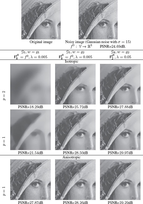
FIGURE 7.3
Isotropic and anisotropic image simplification on a color image with different parameters values of p, λ and different weight functions in local or nonlocal configurations. First row presents the original image. Next rows present simplification results where each row corresponds to a value of p.

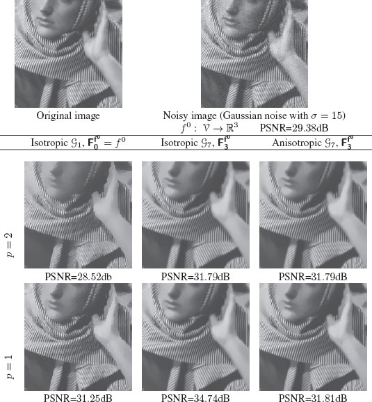
FIGURE 7.4
Isotropic and anisotropic image restoration of a textured image in local and nonlocal configurations with w = g₂, λ = 0.005 and different values of p.

By nature, surface meshes have a graph structure, and we can treat them with our approach. Let $\mathcal{V}$ be a set of mesh vertices, and $ℰ$ be a set of mesh edges. If the input mesh is noisy, we can regularize vertex coordinates or any other function $f^0:\mathcal{V}\subset {ℝ}^3\to {ℝ}^3$ defined on the graph $\mathcal{G}=\left(\mathcal{V},ℰ,w\right)$. Figure 7.6 presents results for a noisy triangular mesh. The simplification enables us to group similar vertices around high curvature regions while preserving sharp angles with p = 1.

To conclude these results for simplification, we consider the USPS data set for which a subset of 100 images from the digits 0 and 1 have been randomly chosen. The selected images are then corrupted independently by Gaussian noise (σ = 40). Figures 7.7(a) and 7.7(b) present the original and corrupted data sets. To associate a graph to the corresponding data set, a 10 Nearest Neighbor Graph (10-NNG) is constructed from the corrupted data set. This graph is depicted in Figure 7.7(c). Each image represents the whole feature vector we want to regularize, i.e., $f^0:\mathcal{V}\to {ℝ}^{16\times 16}$. Figure 7.7 shows the filtering results of p-Laplace isotropic and anisotropic regularization for different values of p ({2, 1}) and λ ({0, 1}). Each result is composed of, with n → ∞: the filtering result (f⁽ⁿ⁾), the difference between the uncorrupted images and the filtered image (|f⁽⁰⁾ – f⁽ⁿ⁾|), the PSNR value between the filtering result and the original uncorrupted image. For p = 2 (with any value of λ) the filtering results are approximatively the same. The processing tends to a uniform data set of two mean digits. This type of processing can be interesting for clustering purposes on the filtered data set where the two classes of digits are more easily distinguishable. From the results, the best PSNR values are obtained with p = 1 and λ = 1, both for the isotropic and the anisotropic regularizations. With these parameters, the filtering better tends to better preserve the initial structure of the manifold while suppressing noise. This effect is accentuated with the use of the anisotropic p-Laplace operator. Finally, the filtering process can be considered as an interesting alternative to methods that consider the preimage problem [54]. The latter methods usually consider the manifold after a projection in a spectral domain by manifold learning [40] to solve the preimage problem [55]. With our approach, the initial manifold is recovered without the use of any projection.

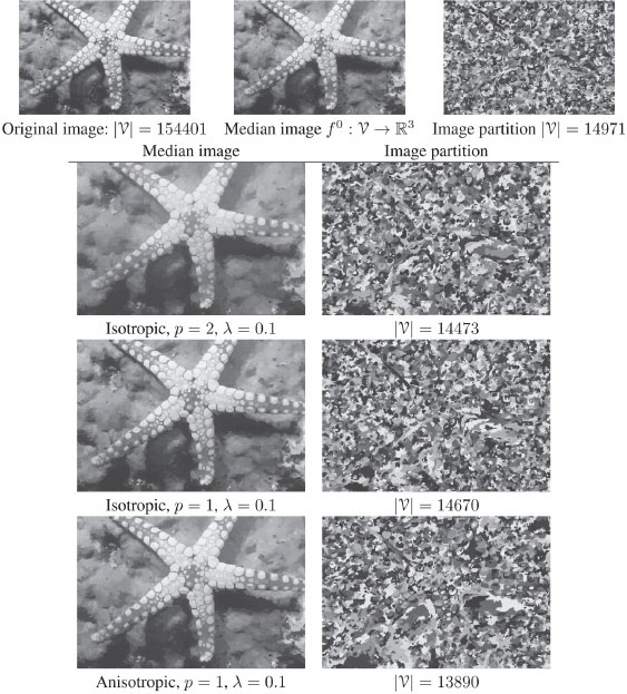
FIGURE 7.5
Image simplification illustration. From an original image, one computes a pre-segmentation and the associated color median image (images in first row). Regularization and decimation are applied on the RAG of the presegmentation and simplified region maps, and color median images are obtained for different values of λ and p with w = g₃.

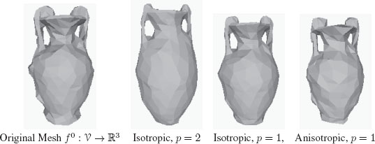
FIGURE 7.6
Triangular mesh simplification illustration. The graph is obtained directly from the mesh and one has $F_0^{f^0}=f^0$, λ = 0.1, w = g₃.

7.5.2    Regularization-Based Interpolation

We illustrate now the abilities of our approach for the interpolation of missing values. We first consider the case of image inpainting. Figure 7.8 presents such inpainting results. The two first rows of Figure 7.8 present results for local inpainting on a 8-adjacency weighted graph (i.e., the diffusion approach) and for nonlocal inpainting on a highly connected graph $\left({\mathcal{G}}_{15}\right)$ with 13 × 13 patches (i.e., the texture replication approach). While the diffusion approach cannot correctly restore the image and produces blurred regions, the texture approach enables an almost perfect interpolation. This simple example shows the advantage of our formulation that combines both geometric and texture inpainting within a single variational formulation. The last row of Figure 7.8 shows that the approach works also for very large areas when the texture is repetitive.

Second, we consider the case of image colorization. Figure 7.9 presents such a result. An initial image is considered with input color scribbles provided by a user. Both local and nonlocal colorization results are satisfactory with an advantage towards nonlocal. Indeed, on the level of the edges, a color blending effect is observed with the local colorization whereas this effect is strongly reduced with nonlocal colorization. This can be seen on the boy’s mouth, hairs and arm. Again, the advantage of our approach resides in the fact that the colorization algorithm is the same for local and nonlocal configurations. Only the graph topology and graph weights are different.

Finally, we consider the case of semi-supervised image segmentation. Figure 7.10 presents results in various configurations. The first column shows the original image, the second column shows the user input labels, and the last column presents the segmentation result. The first row presents a simple example of a color image corrupted by Gaussian noise and composed of two areas. Only two labels are provided by the user, and with a pure local approach on a 4-adjacency grid graph, a perfect result is obtained. Local configurations will provide good results when the objects to be extracted are relatively homogeneous. This is assessed by the results presented in the second row of Figure 7.10. Once the image to be segmented is much more textured, a nonlocal configuration is needed to obtain an accurate segmentation. This is shown in the third row of Figure 7.10 where the 8-adjacency grid graph is augmented with edges from a 4-NNG₃ to capture nonlocal interactions with 7 × 7 patches as feature vectors. The last row of Figure 7.10 shows an example of label diffusion on a graph obtained from a super-pixel segmentation of an image. In this case the graph is the complete graph $K_{\left|\mathcal{V}\right|}$ of the vertices of the RAG corresponding to the super-pixel segmentation. Using the complete graph is not feasible on the whole set of pixels but is computationally efficient on a super-pixel segmentation since the number of vertices is drastically reduced (for this case the reduction factor is of 97%). Using the complete graph for label diffusion has also two strong advantages: the number of input labels is reduced (only one label per type of object to be extracted) and nonadjacent areas can be segmented with the same label even if only one label is provided (this is due to the long range connections induced by the complete graph).

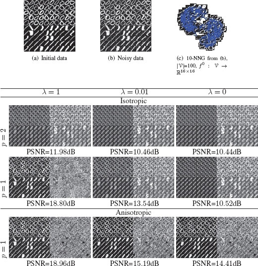
FIGURE 7.7
Isotropic (two first rows) and anisotropic (two last rows) filtering on an image manifold (USPS). Results are obtained with different values of parameters p and λ. Each result shows the filtering result (final f), method noise image (|f⁽⁰⁾ − f⁽ⁿ⁾|) and a PSNR value. (a): original data. (b): noisy data (Gaussian noise with σ = 40), (c): 10-NNG constructed from (b).

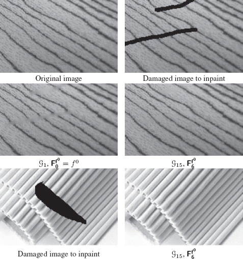
FIGURE 7.8
Isotropic image inpainting with p = 2, w = g₂ in local and nonlocal configurations.

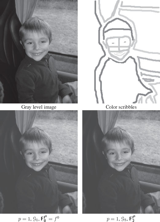
FIGURE 7.9
Isotropic colorization of a grayscale image with w = g₂ and λ = 0.01 in local and nonlocal configurations.

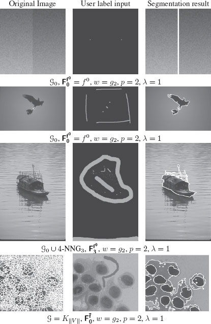
FIGURE 7.10
Semi-supervised segmentation.

7.6    Concluding Remarks

In this chapter we have shown the interest of partial difference equations on graphs for image processing and analysis. As explained in the introduction, PdEs mimic PDEs in domains having a graph structure and enable us to formulate variational problems and associated solutions on graphs of arbitrary topologies. One strong advantage towards using PdE on graphs is the ability to process any discrete data set with the advantage of naturally incorporating nonlocal interactions. We have proposed to use PdE on graphs to define a framework for p-Laplacian regularization on graphs. This framework can be considered as a discrete analogue of continuous regularization models involving PDEs while generalizing and extending them. With various experiments, we have shown the very general situations where this framework can be used for denoising, simplification, segmentation, and interpolation. In future works, other PDEs will be considered, as we have already done by adapting continuous mathematical morphology on graphs with PdEs [15].

Bibliography

[1]  D. Hammond, P. Vandergheynst, and R. Gribonval, “Wavelets on graphs via spectral graph theory,” Appl. Comp. Harmonic Analysis, vol. 30, no. 2, pp. 129 – 150, 2011.

[2]  L. Grady and C. Alvino, “The piecewise smooth Mumford-Shah functional on an arbitrary graph,” IEEE Trans. on Image Processing, vol. 18, no. 11, pp. 2547–2561, Nov. 2009.

[3]  A. Elmoataz, O. Lezoray, and S. Bougleux, “Nonlocal discrete regularization on weighted graphs: a framework for image and manifold processing,” IEEE Transactions on Image Processing, vol. 17, no. 7, pp. 1047–1060, 2008.

[4]  L. Alvarez, F. Guichard, P.-L. Lions, and J.-M. Morel, “Axioms and fundamental equations of image processing,” Archive for Rational Mechanics and Analysis, vol. 123, no. 3, pp. 199–257, 1993.

[5]  T. Chan and J. Shen, Image Processing and Analysis - Variational, PDE, Wavelets, and Stochastic Methods. SIAM, 2005.

[6]  Y.-H. R. Tsai and S. Osher, “Total variation and level set methods in image science,” Acta Numerica, vol. 14, pp. 509–573, mai 2005.

[7]  S. Osher and J. Shen, “Digitized PDE method for data restoration,” in In Analytical-Computational methods in Applied Mathematics, E. G. A. Anastassiou, Ed. Chapman&Hall/CRC, 2000, pp. 751–771.

[8]  J. Neuberger, “Nonlinear elliptic partial difference equations on graphs,” Experiment. Math., vol. 15, no. 1, pp. 91–107, 2006.

[9]  R. Courant, K. Friedrichs, and H. Lewy, “On the partial difference equations of mathematical physics,” Math. Ann., vol. 100, pp. 32–74, 1928.

[10]  L. Grady and J. R. Polimeni, Discrete Calculus - Applied Analysis on Graphs for Computational Science. Springer, 2010.

[11]  A. Bensoussan and J.-L. Menaldi, “Difference equations on weighted graphs,” Journal of Convex Analysis, vol. 12, no. 1, pp. 13–44, 2003.

[12]  J. Friedman and J. Tillich, “Wave equations on graphs and the edge-based Laplacian,” Pacific Journal of Mathematics, vol. 216, no. 2, pp. 229–266, 2004.

[13]  F. Chung and S. T. Yau, “Discrete green’s functions,” Journal of Combinatorial Theory, Series A, vol. 91, no. 1–2, pp. 191–214, 2000.

[14]  R. Hidalgo and M. Godoy Molina, “Navier–stokes equations on weighted graphs,” Complex Analysis and Operator Theory, vol. 4, pp. 525–540, 2010.

[15]  V. Ta, A. Elmoataz, and O. Lezoray, “Partial difference equations on graphs for mathematical morphology operators over images and manifolds,” in IEEE International Conference on Image Processing, 2008, pp. 801–804.

[16]  V. Ta, A. Elmoataz, and O. Lézoray, “Nonlocal pdes-based morphology on weighted graphs for image and data processing,” IEEE Transactions on Image Processing, vol. 20, no. 6, pp. 1504–1516, June 2011.

[17]  V. Ta, A. Elmoataz, and O. Lezoray, “Adaptation of eikonal equation over weighted graphs,” in International Conference on Scale Space Methods and Variational Methods in Computer Vision (SSVM), vol. LNCS 5567, 2009, pp. 187–199.

[18]  A. Elmoataz, O. Lezoray, S. Bougleux, and V. Ta, “Unifying local and nonlocal processing with partial difference operators on weighted graphs,” in International Workshop on Local and Non-Local Approximation in Image Processing (LNLA), 2008, pp. 11–26.

[19]  S. Bougleux, A. Elmoataz, and M. Melkemi, “Discrete regularization on weighted graphs for image and mesh filtering,” in Scale Space and Variational Methods in Computer Vision, ser. LNCS, vol. 4485, 2007, pp. 128–139.

[20]  S. Bougleux, A. Elmoataz, and M. Melkemi, “Local and nonlocal discrete regularization on weighted graphs for image and mesh processing,” International Journal of Computer Vision, vol. 84, no. 2, pp. 220–236, 2009.

[21]  D. Zhou and B. Schölkopf, “Regularization on discrete spaces,” in DAGM Symposium, ser. LNCS, vol. 3663. Springer-Verlag, 2005, pp. 361–368.

[22]  M. Hein, J.-Y. Audibert, and U. von Luxburg, “Graph Laplacians and their convergence on random neighborhood graphs,” Journal of Machine Learning Research, vol. 8, pp. 1325–1368, 2007.

[23]  M. Hein and M. Maier, “Manifold denoising,” in NIPS, 2006, pp. 561–568.

[24]  M. Hein, J.-Y. Audibert, and U. Von Luxburg, “From graphs to manifolds - weak and strong point-wise consistency of graph Laplacians,” in COLT, 2005, pp. 470–485.

[25]  F. R. Chung, “Spectral graph theory,” CBMS Regional Conference Series in Mathematics, vol. 92, pp. 1–212, 1997.

[26]  V.-T. Ta, S. Bougleux, A. Elmoataz, and O. Lezoray, “Nonlocal anisotropic discrete regularization for image, data filtering and clustering,” GREYC CNRS UMR 6072 – Université de Caen Basse-Normandie - ENSICAEN,” HAL Technical Report, 2007.

[27]  M. Belkin and P. Niyogi, “Laplacian eigenmaps for dimensionality reduction and data representation.” Neural Computation, vol. 15, no. 6, pp. 1373–1396, 2003.

[28]  O. Lezoray, V. Ta, and A. Elmoataz, “Manifold and data filtering on graphs,” in International Symposium on Methodologies for Intelligent Systems, International Workshop on Topological Learning, 2009, pp. 19–28.

[29]  T. Bühler and M. Hein, “Spectral clustering based on the graph p-laplacian,” in International Conference on Machine Learning, 2009, pp. 81–88.

[30]  J. O’Rourke and G. Toussaint, “Pattern recognition,” in Handbook of discrete and computational geometry, J. Goodman and J. O’Rourke, Eds. Chapman & Hall/CRC, New York, 2004, ch. 51, pp. 1135–1162.

[31]  A. A. Efros and T. K. Leung, “Texture synthesis by non-parametric sampling,” in International Conference on Computer Vision, vol. 2, 1999, pp. 1033–1038.

[32]  A. Buades, B. Coll, , and J.-M. Morel, “Non-local image and movie denoising,” International Journal of Computer Vision, vol. 76, no. 2, pp. 123–139, 2008.

[33]  G. Gilboa and S. Osher, “Non-local linear image regularization and supervised segmentation,” Multiscale Modeling & Simulation, vol. 6, no. 2, pp. 595–630, 2007.

[34]  A. Chambolle, “An algorithm for total variation minimization and applications,” Journal of Mathematical Imaging and Vision, vol. 20, no. 1–2, pp. 89–97, 2004.

[35]  A. Chambolle and T. Pock, “A first-order primal-dual algorithm for convex problems with applications to imaging,” Journal of Mathematical Imaging and Vision, vol. 40, no. 1, pp. 120–145, 2011.

[36]  C. Tomasi and R. Manduchi, “Bilateral filtering for gray and color images,” in International Conference on Computer Vision. IEEE Computer Society, 1998, pp. 839–846.

[37]  T. Chan, S. Osher, and J. Shen, “The digital TV filter and nonlinear denoising,” IEEE Transactions on Image Processing, vol. 10, no. 2, pp. 231–241, 2001.

[38]  G. Gilboa and S. Osher, “Nonlocal operators with applications to image processing,” UCLA, Tech. Rep. CAM Report 07–23, July 2007.

[39]  G. Gilboa and S. Osher, “Nonlocal operators with applications to image processing,” Multiscale Modeling & Simulation, vol. 7, no. 3, pp. 1005–1028, 2008.

[40]  R. Coifman, S. Lafon, A. Lee, M. Maggioni, B. Nadler, F. Warner, and S. Zucker, “Geometric diffusions as a tool for harmonic analysis and structure definition of data,” Proc. of the National Academy of Sciences, vol. 102, no. 21, pp. 7426–7431, 2005.

[41]  F. Wang, J. Wang, C. Zhang, and H. C. Shen, “Semi-Supervised Classification Using Linear Neighborhood Propagation,” IEEE Computer Society Conference on Computer Vision and Pattern Recognition - Volume 1 (CVPR’06), vol. 1, pp. 160–167, 2006.

[42]  L. Grady, “Random walks for image segmentation,” IEEE Transactions on Pattern Analysis and Machine Intelligencen, vol. 28, no. 11, pp. 1768–1783, 2006.

[43]  A. K. Sinop and L. Grady, “A Seeded Image Segmentation Framework Unifying Graph Cuts And Random Walker Which Yields A New Algorithm,” in International Conference on Computer Vision, 2007, pp. 1–8.

[44]  C. Couprie, L. Grady, L. Najman, and H. Talbot, “Power watersheds: A new image segmentation framework extending graph cuts, random walker and optimal spanning forest,” in International Conference on Computer Vision, Sept. 2009, pp. 731–738.

[45]  M. Belkin, P. Niyogi, V. Sindhwani, and P. Bartlett, “Manifold Regularization: A Geometric Framework for Learning from Labeled and Unlabeled Examples,” Journal of Machine Learning Research, vol. 7, pp. 2399–2434, 2006.

[46]  V.-T. Ta, O. Lezoray, A. Elmoataz, and S. Schüpp, “Graph-based tools for microscopic cellular image segmentation,” Pattern Recognition, vol. 42, no. 6, pp. 1113–1125, 2009.

[47]  M. Bertalmío, G. Sapiro, V. Caselles, and C. Ballester, “Image inpainting,” in SIGGRAPH, 2000, pp. 417–424.

[48]  M. Ghoniem, Y. Chahir, and A. Elmoataz, “Geometric and texture inpainting based on discrete regularization on graphs,” in ICIP, 2009, pp. 1349–1352.

[49]  G. Facciolo, P. Arias, V. Caselles, and G. Sapiro, “Exemplar-based interpolation of sparsely sampled images,” in EMMCVPR, 2009, pp. 331–344.

[50]  A. Levin, D. Lischinski, and Y. Weiss, “Colorization using optimization,” ACM Transactions on Graphics, vol. 23, no. 3, pp. 689–694, 2004.

[51]  L. Yatziv and G. Sapiro, “Fast image and video colorization using chrominance blending,” IEEE Transactions on Image Processing, vol. 15, no. 5, pp. 1120–1129, 2006.

[52]  O. Lezoray, A. Elmoataz, and V. Ta, “Nonlocal graph regularization for image colorization,” in International Conference on Pattern Recognition (ICPR), 2008.

[53]  A. Levinshtein, A. Stere, K. N. Kutulakos, D. J. Fleet, S. J. Dickinson, and K. Siddiqi, “Turbopixels: Fast superpixels using geometric flows,” IEEE Transactions on Pattern Analysis and Machine Intelligence, vol. 31, pp. 2290–2297, 2009.

[54]  J. T. Kwok and I. W. Tsang, “The pre-image problem in kernel methods,” in International Conference on Machine Learning, 2003, pp. 408–415.

[55]  N. Thorstensen, F. Segonne, and R. Keriven, “Preimage as karcher mean using diffusion maps : Application to shape and image denoising,” in Proceedings of International Conference on Scale Space and Variational Methods in Computer Vision, ser. LNCS, Springer, Ed., vol. 5567, 2009, pp. 721–732.

¹Since graphs are considered undirected, if $e_{ij}\in ℰ$, then $e_{ji}\in ℰ$.