
The Role of Graphs in Matching Shapes and in Categorization
Brown University
School of Engineering
Providence, Rhode Island, USA
CONTENTS
14.2 Using Shock Graphs for Shape Matching
14.3 Using Proximity Graphs for Categorization
14.3.1 Indexing: Euclidean versus Metric Spaces
14.3.2 Metric-based Indexing Methods
14.3.3 Capturing the Local Topology
This chapter explores the value of graphs in computer vision from the perspective of representing both structural quantum variations as well as metric changes, as applied to the matching and categorization problems. It briefly overviews our particular approach in using shock graphs in matching and recognition, and proximity graphs in categorization. The key concept is that graphs can be viewed as capturing a notion of discrete topology, whether it is related to the shape space or to the category space. Specifically, we view both shape matching and categorization as establishing first a similarity space. Subsequently, the cost of a “geodesic” from one point to another is computed as the internal of dissimilarity over this path. The technology for shape matching uses shock graphs, a form of the medial axis, while the technology for categorization uses proximity graphs.
Graphs are ubiquitous in computer vision, as evidenced by the large body of work that is presented and referenced in this book. Some insight into why this is the case can be obtained by observing that the set of images arising from an equivalence class of objects, e.g., horses, are affected by a vast variety of visual transformations such as changes in illumination, pose, and viewing distance, occlusion, articulation, within category type variation, camera gain control, interaction with background clutter, and others. The sorting out of commonalities from among such an incredible variety of variations to establish an equivalence class is certainly an incredible feat, one that our visual system solves on a regular basis.
The regularity of objects, in contrast, places them in a low-dimensional space embedded in a very high-dimensional image space. Even within this low-dimensional space the distribution of object representations is not uniform. Rather, in the similarity space, objects from the same class are clustered and arranged as a cluster in a neighborhood of similar categories, see; Figure 14.1. This implies that in an arbitrary path traversing an exemplar from one category to an exemplar from another category, say from a giraffe to a horse, two distinct types of events can be observed: initially a giraffe’s deformation may lead us to other giraffe exemplars, but eventually as the deformation varies in type and magnitude we venture into noncategory exemplars before we finally arrive at a horse exemplar. This typifies the dual nature of our observations in general in computer vision, one quantitative and metric, and one structural and in quantum steps. This dual nature is one of the key challenges underlying the success of computer vision algorithms: Optimizing a functional is metric and usually assumes a uniform structure, while what is required is optimizing over both quantum changes and metric variations. Herein lies the intrinsic value of an attributed graph as a representation: it embodies both these aspects.
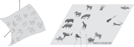
FIGURE 14.1
(Left) A cartoon view of the space of observable of images, shapes, categories, etc. as lying on a low-dimensional manifold embedded in a very high-dimensional space. The structure of these abstract points when arranged in an appropriate similarity space is inherently clustered, reflecting the nature of objects and categories, as highlighted for the space of categories on the right. (Right) The similarity space of categories naturally reflects the topology of categories at the basic, super- and sub-levels of categorization, and clustering of exemplar categories.
Jan Koenderink observed a fundamental point about the use of representations for shape matching, that representations of shape can be either static of dynamic [1]. In a static representation, each shape maps to a point in some abstract space, e.g., a high-dimensional Euclidean feature space. Two shapes are then matched by measuring the distance between the two representation, e.g., using the Euclidean distance, in the representation space. In contrast, in a dynamic representation, the matching of two points is not done by measuring distance in the representation space, but rather it is based on the cost of deforming one representation to another in an intrinsic manner1. The cost itself is computed by summing up the cost of deforming each shape to a neighboring shape, thus requiring a basic, atomic cost for comparing two infinitesimally close shapes. The deformation cost can then be viewed as the cost of the geodesic between two shapes in an underlying similarity space. This is equally true for a category space. The critical advantage of a dynamic representation is that it only allows for the transformations which are legal, in contrast to infeasible transformations implicitly represented in a static space. Furthermore, the straight line in the embedding space may not be the appropriate geodesic when we consider the requirements of matching. For example, it may not traverse or correspond to “legal” shapes.
The framework presented is based on these ideas and is fairly general. The basic ingredients are visual constructs such as shapes, categories, image fragments, etc. These constructs are assumed to have an inherent sense of similarity which can then be used to define a continuous space as above. The next step is to find the optimal geodesic connecting two points whose cost defines a global sense of similarity. Such an approach, however, must consider that for any practical implementation the similarity space must be discretized so that the geodesic path costs can be computed in a realistic manner. Such a discretization requires three steps:
1. Definition of an equivalence class for the points (shapes, categories, etc.) in the underlying space;
2. Definition of which equivalence classes are immediate neighbors;
3. Definition of an atomic costs for transitioning from one equivalence class to another.
This structure converts the original continuous space to a discrete one, one which can be effectively represented by an attributed graph: each equivalence class is a node of the graph, while each immediate neighbor defines a link or an edge in the graph. Attributing each graph link with a cost allows for the computation of costs for each geodesic path by summation. We now illustrate the construction of this structure in the context of two examples, one for matching shapes for recognition and one for representing categorization for indexing.
14.2 Using Shock Graphs for Shape Matching
While the word shape or form has a strongly intuitive meaning to us, Figure 14.2, the construction of such a concept in computer vision has been elusive. Shape is multifaceted [2]: (1) it simultaneously involves a representation of the shape silhouette as well as the shape interior. Concepts such as the contour tangents are explicit in one and implicit in the other, and vice versa for a “neck”; (2) shape involves local attributes as well as global attributes; (3) shape can be thought of being made as hierarchy of parts or as whole; (4) shape can be perceived at various scales. A representation of such a complex notion by a simple collection of features embedded in a high-dimensional Euclidean space would be hard-pressed to capture the subtly of shape.
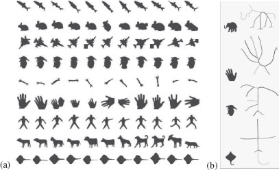
FIGURE 14.2
a) A database of shapes which has been popular in gauging the performance of shape matching algorithms. b) The shock graph of a few shapes is illustrated partially by showing the decomposition of shock segments, but not the shock dynamics.
Our approach to shape is based the shock-graph, a variant of the medial axis. Formally, the medial axis is the closure of centers of circles with at least two points of tangency to the contour of the shape. A classic construction of the medial axis is as the quench points of “grassfire”, when the shape is considered as field of grass with fire initiated at the shape boundary [3]. In this wave propagation analogy, the medial axis can also be viewed as the shock points of the evolving front [4, 2]. In this case, each shock point has a dynamic associated with it that allows a finer classification than that allowed by the static view of the medial axis; some points are sources of flow, others are sinks of flow, and some other are junctures of flow, with continuously flowing segments connecting them. This leads to a formal definition of a shock graph as a directed graph with nodes representing flow sources, sinks, and junctions, while links are continuous segments connecting these. See [5] for a formal classification of the local form of shock points, [6] for its use in 2D recognition, [7] for 3D recognition, and [8] for top-down model-based segmentation; examples are illustrated in Figure 14.2b. Observe that this dynamic view of a shock graph allows for a geometrical decomposition of medial axis into finer branches, leading to a qualitatively more informative description. Given a medial axis sketch one gets a coarse idea of the equivalence class of shapes that gave rise to it, but given a shock graph this class is much better defined. That the topology of the shock graph, without any metric information, captures the categorical structure of the shape is a critical element in its success in shape recognition. The actual dynamics of shock propagation on the shock graph then provides the metric structure for its reconstruction [5]. The shock graph topology provides the answer to the first of the three steps described in the introduction:
Definition 14.2.1
Two shapes are said to be equivalent if they share the same shock graph topology. A shape cell is the set of all shapes that share the same shock graph topology.
This shape cell provides a discretization of the shape space into equivalence classes of shapes.
The second step in the process is based on the instabilities of the representation. Any representation involves such instabilities or transitions, which are defined as points where the shape undergoes an infinitesimally small smooth perturbation and the representation undergoes a structural change. This is unstable because a small change in the shape causes a large change in the representation. Every representation experiences such instabilities, e.g., representing the boundary of a shape with a polygon, etc. These instabilities define the neighborhood structure of a shape cell, Figure 14.3(a); the shapes in a shape cell as they deform near the instability may venture into a different distinct shape cell. Thus two shape cells are neighbors if the shapes in one can be transformed to shapes in the other by one single transition, aside from continuous deformations. The equivalence class of paths that goes through the same shape cells can then provide a recipe for the second discretization step:
Definition 14.2.2
Two deformations paths are equivalent if they traverse the same ordered set of shape cells, Figure 14.3(b).
The third component of our approach is an atomic cost for going from one shape cell to another. The cost of deforming two very close shapes when structural correspondences are not an issue is easier to define. For example one can use the Hausdorff metric or a variant. We have in the past used a measure which penalized differences in the geometric and dynamic attributes of the shock graph [6]. The search over all such paths leads to the geodesic, the path of least cost, which defines the metric of dissimilarity between two shapes, Figure 14.3(c).
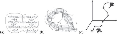
FIGURE 14.3
From [6]: (a) Each of the two sets of shapes define a shape cell. The two shapes cells are immediate neighbors. (b) The set of paths from shape A to shape B can be grouped into equivalent classes of paths, where two paths are equivalent if they are composed of the same sequence of transitions. c) The geodesic between two shapes is then the path of least cost, and this cost defines the dissimilarity between two shapes.
With such a three-step discretization of the shape space, all that is left to do is to examine all equivalent classes of deformation paths from one shape to another. One more important aspect that keeps the problem finite without any loss of generality is to avoid considering paths which unnecessarily venture into complexity and then back towards simplicity. This can be done by splitting the full path between two shapes into two paths of nonincreasing complexity, as in Figure 14.4(a). The full space is therefore structured as two finite trees with each having one of the two shapes at the root, as in Figure 14.4(b); the two trees have many nodes which are equivalent. Our task is to search for the least cost path, Figure 14.4(c), the geodesic, by searching through this space, which can be graphically represented.
An approach to the efficient search of this space is by dynamic programming, which requires an adaptation into the domain of shock graphs. Specifically, each instability or transition of the shock graph can be thought of as an edit in the graph domain. We have therefore developed an edit distance for shock graphs that runs in polynomial time and refer the read to the following papers for detail [9, 10, 6]. The solution generates the optimal path of deformation and a similarity based cost which we regard as the distance between two shapes, as in Figure 14.5. This distance has been effectively used for shape matching as illustrated on multiple datasets [6]. Figure 14.6 shows shape recognition performance on the Kimia-99 and Kimia-216 shape databases [11].
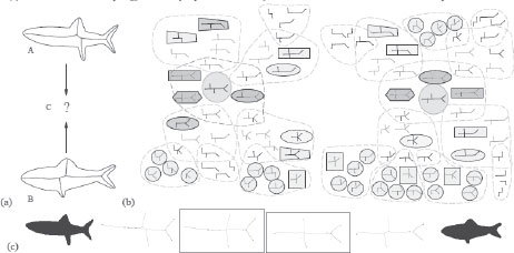
FIGURE 14.4
From [6]: (a) Two shapes and their shock graphs. (b) The set of possible equivalent classes of deformation paths from one fish to another is illustrated. (c) The optimal path involves one transition for each shape in this case. In general, however, the geodesic involves many more transitions.
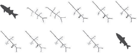
FIGURE 14.5
The sequence of edits which optimally transform one fish into another through operations on the shock graph.
14.3 Using Proximity Graphs for Categorization
A second example that illustrates the use of graphs for capturing the local topology of a similarity space is the categorization task2 The successful experience in building an explicit structure for the shape space by using a local similarity and neighborhood structure, as described in the previous section, motivates the construction of a similar structure for the spaces of abstract categories, denoted as space X. Our assumption is that we can define a metric of dissimilarity d for any pair of points in X, expecting it to be meaningful when the categories are fairly similar, but not necessarily meaningful when they are not. Given a query q, the proximity search task is to find its closest neighbors or neighbors within a given range. Typically, the computation of the metric is expensive so that the O(N) computation of d(q, xi), where xi is one of N sample points in the metric space X, is not feasible without some form of index structure [12, 13, 14, 15]. The key insight here is to represent a metric space via a proximity graph and use this discrete topology to construct a hierarchical index to allow for sublinear search, while allowing for dynamic insertion and deletion of points for incremental learning.
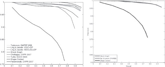
FIGURE 14.6
The recognition performance of the shock-graph matching based on the approach described above for the Kimia-99 and Kimia-216 shape databases [11].
14.3.1 Indexing: Euclidean versus Metric Spaces
There is a significant difference between indexing into a Euclidean space and a general metric space, especially when the latter is intrinsically high-dimensional. In general, indexing into Euclidean spaces relies on classical spatial access methods such as KD-tree [16], R-tree [17], and Quadtree [18], with a long history of use in computer vision, e.g., [19, 20]. However, when objects cannot be represented as points in a Euclidean space, a low-distortion embedding is often used, e.g., the Karhunen-Loeve transform [21], PCA [22], MDS [23, 24], random projections [25, 26, 27], to approximate a metric space. Unfortunately, a low-distortion embedding for the shape space requires a very high-dimensional global space: using the shape similarity metric described earlier, the hammer (square) and bird (diamond) categories are well separated in R2, but the addition of keys (triangle) now requires three dimensions, Figure 14.7. This trend continues with more categories so that the embedding becomes practical beyond a few categories. It is well-known that the search becomes intractable beyond 10–20 dimensions due to the curse of dimensionality [28, 29]. Thus, Euclidean spatial access methods are not appropriate for our applications.
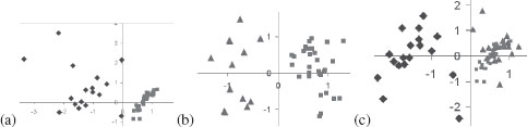
FIGURE 14.7
The required embedding dimension for many categories is high: Two dimensions suffice for embedding the categories of hammer and bird (a) (this is done by standard MDS), or hammer and keys (b), but the three categories of hammer, keys, and birds require an additional dimension. This increase in dimensions with the addition of new categories continues at a sub-linear rate, but the resulting dimensions is very high.
14.3.2 Metric-based Indexing Methods
Metric-based indexing methods go back to Burkhard and Keller [30], and typically use the triangle inequality and the classical divide-and-conquer approach [31, 32, 33, 34, 35, 36, 37, 32, 30, 38, 33]; see [39] for a review. Metric-based indexing methods are typically either based on pivots or on clustering. Pivot-based algorithms use the distance from query to a set of distinguished elements (pivots or prototypes).The triangle inequality is used to discard elements represented by the pivot without necessarily computing a distance to query. These algorithms generally improve as more pivots are added, although the space requirements of the indexes increase as well.
Clustering or compact partitioning algorithms divide the set into spatial zones as compact as possible, either by Voronoi type regions delimited by hyperplanes [33, 34, 35] or a covering radius [36, 37] or both [32]. They are able to discard complete zones by performing few distance evaluations between the query q and a centroid of the zone. The partition into zones can be hierarchical, but the indexes use a fixed amount of memory and do not improve by having more space. As shown in [14], compact partitioning algorithms deal better with high dimensional metric spaces, with pivot-based system becoming impractical beyond dimension 20.
We have explored the use of exact metric-based methods and have shown that they have poor indexing efficiency for our application [41] where the best indexing efficiency among the VP-tree [33, 38], AESA [42], unbalanced BK-tree [43], GH-tree [33], and GNAT [32] on a database of shapes achieved savings of 39% of the computations for AESA, not nearly enough to tackle much larger databases. A key issue underlying poor indexing is the high-dimensionality of data, indicated by a peaky histogram, Figure 14.8. As the intrinsic data dimensionality increases, indexes lose their efficiency since all the elements are more or less at the same distance from each other. Intuitively, pivot-based methods define “rings” of points at the same distance around pivots. The intersections of rings define the zones in which the space is partitioned, which need to remain spatially compact as the dimension grows, requiring numerous rings and therefore pivots. Compact partitioning by construction defines compact regions and requires no additional memory; It is easier to prove that a compact region is far enough from the query than to do the same for a sparse region. This may explain why AESA had the best performance in our applications.
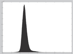
FIGURE 14.8
The intrinsic dimensionality of a shape dataset is revealed by the “peakiness” of the histogram of distances between pairs of shape. Specifically [31, 40] defines intrinsic dimensionality of a metric space as , where μ and σ2 are the mean and variance of its histogram of distances. The histogram of pairwise distanced for the MPEG7 shape dataset gives an intrinsic dimensionality of 22. This number is quite high for such a relatively small dataset of 70 categories and 20 exemplars per category, when compared to a realistic situation.
Another class of recent methods, nonlinear dimensionality reduction (NDR), applies when the data lives in a high-dimensional space but lies on a low-dimensional manifold [44, 45, 46]. In [44] the “geodesic” distance between two points is estimated by limiting the interaction of each point to its knearest neighbors, and then MDS is applied. In [45, 46] each point is described as a weighted combination of its k-nearest neighbors. Both techniques assume a uniform distribution over the manifold and suffer when this assumption is violated. Indeed, our preliminary results using the ISOMAP [44] on our 1032 shape database showed that while the idea of limiting the interaction of each shape to a local neighborhood is useful, such demands should not be made globally.
We have earlier explored [41] a wave propagation approach to use a kNN graph connecting each shape to its k-nearest neighbors (see a summary of our approach in [47], pages 637-641) and used a number of exemplars as initial seeds for a wave propagation-based search. The multiply connected front propagated only from its closest point to the query. This rather simple method doubled the performance from 39% to 78% [41]. While this is encouraging and significant, this level of savings is not yet nearly sufficient for practical indexing into millions of fragments and thousands of categories. What is lacking is a method to capture local topology as described below.
14.3.3 Capturing the Local Topology
Exact metric search methods have focused their attention on the triangle inequality, which is weak in a high-dimensional space for partitioning space for access. Our spaces, however, enjoy an additional underlying structure which can be exploited, namely, a “manifold” structure, speaking in intuitive terms. Visual objects and categories are not randomly distributed, but are highly clustered and have lower dimensionality than their embedding spaces. As in NDR methods above, capturing local topology is a first step towards defining such a structure. Specifically, with an explicit local topology, we can define the notion of propagation and wavefront. This allows us to define Euclidean-like concepts such as direction. Given a point and a front around this point, the ordering of points along the front defines a sense of direction. This sense of direction is very important in Euclidean spaces as it helps avoid further search in a direction that takes us away from the query. Metric spaces which do not have a sense of direction are at a great loss, having to rely on the much weaker triangle inequality.
The need for a local topology arises for other reasons as well. Second, the metric of similarity we define, e.g., between fragments and categories, only makes sense when the two points are close to each other: we can define the distance between a horse and a donkey and compare it in a meaningful way to the distance between a horse and a zebra. But how can the distance between a horse and a clock be meaningfully related to the distance between a horse and a scorpion? We argue that a proper notion of distance between two points should be built as the geodesic distance between the two points built up from and grounded on distances between nearby points. This approach has paid off in our experience with shape recognition as discussed in the previous section. Third, an idea from the cognitive science community, “categorical perception”, argues that the similarity space is warped so as to optimally differentiate between neighboring categories [48]. The local representation of topology would allow a selective “stretching” of the underlying space! Fourth, our experiments also reveal that in cases where close by shapes from two distinct categories were clustered, e.g., a bird and a flying dinosaur, consideration of distances to third parties could reveal the distinction. This idea of using higher-order local structures by maintaining k-tuple structure is akin to the concept of volume preserving embedding which suggests that not only pairwise distances but also volumes must be preserved [49]. This is applicable when local topology is explicitly represented.
The kNN approach in defining a neighborhood in NDR is successful when data is uniformly distributed, but fails in clustered data. This was clearly demonstrated by the barbell configuration shown in [46]. What is lacking in the kNN approach is that (i) the space is often disconnected, and (ii) not all local directions are captured such that there are “holes” in the kNN’s idea of a neighborhood.
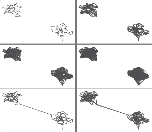
FIGURE 14.9
In the first two rows, the kNN graph is shown for reasonable values of k = 1, 5, 10, 15, which are all disconnected. In contrast, the bottom row shows the RNG and GG graphs which are connected between the two clusters. Of course for very high values of k the kNN graph is connected, but at this point the kNN graph is close to a complete graph, thus defeating any efficiency gains.
Capturing the local topology with proximity graphs. Alternatively, we suggest that the proper method to capture local topology is to use proximity graphs [50, 51], in particular the β-skeleton and the Gabriel graphs, which capture the spatial distribution of points rather than their distance-based ranking. These graphs are connected and avoid the drawback with the use of k-nearest neighbor as a local neighborhood that does not fully “fill the space” around each point when it is close to a category boundary (e.g., key versus hammer) because the nearest neighbors are all on one side, as in Figure 14.9. The geodesic paths on the Gabriel graph, in particular, have minimal distortion. Another advantage of proximity graphs is that they allow for incremental update and deletion since the construction is by nature local.
Proximity graphs are a class of graphs that represent the neighborhood relationship among a set of N exemplar points, X* = {xi, i = 1, ···, N} in a metric space (X, d). In the following, we consider graphs whose nodes (vertices) are xi and where the links between nodes establish a neighborhood of proximity relationship between the nodes. For this reason, these graphs can be described as proximity graphs or sometimes geometric graphs. In this class fall well-known graphs such as the nearest neighbor graph, Delaunay triangulation (DT) graphs, minimal spanning tree (MST), and also the less well-known graphs such as the relative neighborhood graph (RNG), the Gabriel graph, and β–skeleton graphs.
Definition 14.3.1
The nearest neighbor (NN) of a point xi is the point xj, i ≠ j, that minimizes d(xi, xj). When two points ore more have equal minimal distances to xi, the point with the maximum index is chosen to break the tie. The nearest neighbor is denoted as NN(xi). The nearest neighborhood graph (NNG) is a directed graph where each point xi is connected to its nearest neighbor [52]. The k-nearest neighborhood graph (kNN) is a directed graph where each point xi is connected to the k closest points to it.
Definition 14.3.2
The relative neighborhood graph (RNG) [53] of a set of points X* is a graph such that vertices xi ∈ X* and xj ∈ X* are connected with an edge if and only if there exists no points xk ∈ X* for which
(14.1) |
Definition 14.3.3
The Gabriel graph (GG) [54] of a set of points X* is a graph such that two vertices xi ∈ X * and xj ∈ X* are connected with an edge if and only if for all other points xk ∈ X* we have
(14.2) |
Definition 14.3.4
The β-skeleton graph (BSG) [55] of a set of points X* is a graph such that two vertices xi ∈ X* and xj ∈ X* are connected with an edge if and only if for all other points xk ∈ X* we have
(14.3) |
(14.4) |
Note that the radius of the circles that make up the lune are .
β–skeletons were first defined by Kirkpatrick and Radke (1985) [55] as a scale-invariant extension of the alpha-shapes of [56]. The behavior of the β–skeleton graph as β varies continuously from 0 to ∞ is to form a sequence of graphs extending from the complete graph to the empty graph. There are also special cases: β = 1 leads to the Gabriel graph, which is known to contain the Euclidean minimum spanning tree in the plane. β = 2 gives the RNG. A generalization to γ–graphs can be found in [57].
There is an interesting interpretation of the β–skeletons to the support vector machines (SVM) in the context of solving a geometric classification problem [58, 59].
Observation: It should be noted that NNG ⊂ RNG ⊂ GG ⊂ DT.
Also note that the Gabriel graph is a subgraph of the Delaunay triangulation; it can be found in linear time if the Delaunay triangulation is given [60]. The Gabriel graph contains as a subgraph the Euclidean minimum spanning tree and the nearest neighbor graph. It is an instance of a beta-skeleton.
Figure 14.10 shows the comparison of proximity graphs to the kNN graphs in this context. We expect that proximity graphs will see increasing use in computer vision as a way of capturing the local topology.
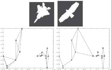
FIGURE 14.10
(top) A difficult case for capturing the local topology using the locally linear embedding from [46]. (bottom) The kNN versus proximity graph connectivity.
Graphs are ideal structures to capture the local topology among points in a space. We have covered two examples. The first example uses shock graphs, which capture the local topology of shape parts. The second example uses proximity graphs, which capture the local topology of a similarity space. The work also provides a template for generalizing this work to any space where the notions of local similarity and of equivalence class make sense.
The author gratefully acknowledges the support of NSF grant IIS-0083231 in funding research leading to this article.
[1] J. J. Koenderink and A. J. van Doorn, “Dynamic shape,” Biological Cybernetics, vol. 53, pp. 383–396, 1986.
[2] B. B. Kimia, A. R. Tannenbaum, and S. W. Zucker, “Shapes, shocks, and deformations, I: The components of shape and the reaction-diffusion space,” International Journal of Computer Vision, vol. 15, no. 3, pp. 189–224, 1995.
[3] H. Blum, “Biological shape and visual science,” J. Theor. Biol., vol. 38, pp. 205–287, 1973.
[4] B. B. Kimia, A. R. Tannenbaum, and S. W. Zucker, “Toward a computational theory of shape: An overview,” in European Conference on Computer Vision, 1990, pp. 402–407.
[5] P. J. Giblin and B. B. Kimia, “On the intrinsic reconstruction of shape from its symmetries,” IEEE Trans. on Pattern Anal. Mach. Intell., vol. 25, no. 7, pp. 895–911, July 2003.
[6] T. Sebastian, P. Klein, and B. Kimia, “Recognition of shapes by editing their shock graphs,” IEEE Trans. on Pattern Anal. Mach. Intell., vol. 26, pp. 551–571, May 2004.
[7] C. M. Cyr and B. B. Kimia, “A similarity-based aspect-graph approach to 3D object recognition,” International Journal of Computer Vision, vol. 57, no. 1, pp. 5–22, April 2004.
[8] N. H. Trinh and B. B. Kimia, “Skeleton search: Category-specific object recognition and segmentation using a skeletal shape model,” International Journal of Computer Vision, vol. 94, no. 2, pp. 215–240, 2011.
[9] P. Klein, S. Tirthapura, D. Sharvit, and B. Kimia, “A tree-edit distance algorithm for comparing simple, closed shapes,” in Tenth Annual ACM-SIAM Symposium on Discrete Algorithms (SODA), San Francisco, California, January 9-11 2000, pp. 696–704.
[10] P. Klein, T. Sebastian, and B. Kimia, “Shape matching using edit-distance: an implementation,” in Twelfth Annual ACM-SIAM Symposium on Discrete Algorithms (SODA), Washington, D.C., January 7–9 2001, pp. 781–790.
[11] B. Kimia. (2011) Shape databases. [Online]. Available: http://vision.lems.brown.edu/content/available-software-and-databases
[12] G. R. Hjaltason and H. Samet, “Contractive embedding methods for similarity searching in metric spaces,” CS Department, Univ. of Maryland, Tech. Rep. TR-4102, 2000.
[13] ——, “Properties of embedding methods for similarity searching in metric spaces,” IEEE Trans. Pattern Anal. Mach. Intell., vol. 25, no. 5, pp. 530–549, 2003.
[14] E. Chavez, G. Navarro, R. Baeza-Yates, and J. L. Marroquín, “Searching in metric spaces,” ACM Computing Surveys, vol. 33, no. 3, pp. 273 – 321, September 2001.
[15] G. Navarro, “Analyzing metric space indexes: What for?” in Proc. 2nd International Workshop on Similarity Search and Applications (SISAP). IEEE CS Press, 2009, pp. 3–10, invited paper.
[16] J. L. Bentley and J. H. Friedman, “Data structures for range searching,” ACM Computing Surveys, vol. 11, no. 4, pp. 397–409, Decmber 1979.
[17] A. Guttman, “R-tree: A dynamic index structure for spatial searching,” in Proceedings of the 1984 ACM SIGMOD International Conference on Management of Data, 1984, pp. 47–57.
[18] H. Samet, “The quadtree and related hierarchical data structures,” ACM Computing Surveys, vol. 16, no. 2, pp. 187–260, 1984.
[19] O. Boiman, E. Shechtman, and M. Irani, “In defense of nearest-neighbor based image classification,” in CVPR, 2008.
[20] N. Kumar, L. Zhang, and S. K. Nayar, “What is a good nearest neighbors algorithm for finding similar patches in images?” in European Conference on Computer Vision, 2008, pp. 364–378.
[21] D. Cremers, S. Osher, and S. Soatto, “Kernel density estimation and intrinsic alignment for shape priors in level set segmentation.” International Journal of Computer Vision, vol. 69, no. 3, pp. 335–351, 2006.
[22] D. Comaniciu and P. Meer, “Mean shift: a robust approach toward feature space analysis,” IEEE Trans. on Pattern Anal. Mach. Intell., vol. 24, no. 5, pp. 603–619, 2002.
[23] T. F. Cox and M. A. A. Cox, Multidimensional Scaling. Chapman and Hall, 1994.
[24] J. B. Kruskal and M. Wish, Multidimensional Scaling. Beverly Hills, CA: Sage Publications, 1978.
[25] D. Achlioptas, “Database-friendly random projections,” in Symposium on Principles of Database Systems, 2001. [Online]. Available: www.citeseer.nj.nec.com/achlioptas01databasefriendly.html
[26] E. Bingham and H. Mannila, “Random projection in dimensionality reduction: Applications to image and text data,” in Proceedings of the ACM SIGKDD International Conference on Knowledge Discovery and Data Mining, San Francisco, CA, Aug. 2001, pp. 245–250.
[27] N. Gershenfeld, The Nature of Mathematical Modelling. Cambridge: Cambridge University Press, 1999.
[28] R. Weber, “Similarity search in high-dimensional data spaces,” in Grundlagen von Datenbanken, 1998, pp. 138–142. [Online]. Available: www.citeseer.nj.nec.com/111967.html
[29] C. Böhm, S. Berchtold, and D. A. Keim, “Searching in high-dimensional spaces: Index structures for improving the performance of multimedia databases,” ACM Comput. Surv., vol. 33, no. 3, pp. 322–373, 2001.
[30] W. Burkhard and R. Keller, “Some approaches to best-match file searching,” Communications of the ACM, vol. 16, no. 4, pp. 230–236, 1973.
[31] E. Chavez, G. Navarro, R. Baeza-Yates, and J. Marroquin, “Searching in metric spaces,” ACM Computing Surveys, vol. 33, no. 3, pp. 273–321, September 2001.
[32] S. Brin, “Near neighbor search in large metric spaces,” in Proc. Intl. Conf. on Very Large Databases (VLDB), 1995, pp. 574–584. [Online]. Available: www.citeseer.nj.nec.com/brin95near.html
[33] J. Uhlmann, “Satisfying general proximity/similarity queries with metric trees,” Information Processing Letters, vol. 40, pp. 175–179, 1991.
[34] H. Nolteimer, K. Verbarg, and C. Zirkelbach, “Monotonous bisector trees – a tool for efficient partitioning of complex scenes of geometric objects.” in Data Structures and Efficient Algorithms, Lecture Notes in Computer Science, vol. 594, 1992, pp. 186–203.
[35] F. Dehne and H. Nolteimer, “Voronoi trees and clustering problems.” Information Systems, vol. 12, no. 2, pp. 171–175, 1987.
[36] E. Chavez and G. Navarro, “An effective clustering algorithm to index high dimensional metric spaces.” in Proc. 7th International Symposium on String Processing and Information Retrieval (SPIRE’00). IEEE CS Press, 2000, pp. 75–86.
[37] P. Ciaccia, M. Patella, and P. Zezula, “M-tree: an efficient access method for similarity search in metric spaces.” in Proc. 23rd Conference on Very Large Databases (VLDB’97), 1997, pp. 426–435.
[38] P. Yianilos, “Data structures and algorithms for nearest neighbor search in general metric spaces,” in ACM-SIAM Symposium on Discrete Algorithms, 1993, pp. 311–321.
[39] H. Samet, The design and analysis of Spatial Data Structures. Addison-Wesley, MA, 1990.
[40] E. Chavez and G. Navarro, “A compact space decomposition for effective metric indexing,” Pattern Recognition Letters, vol. 26, no. 9, pp. 1363–1376, 2005.
[41] T. B. Sebastian and B. B. Kimia, “Metric-based shape retrieval in large databases,” in International Conference on Pattern Recognition, vol. 3, 2002, pp. 30 291–30 296.
[42] E. Vidal, “An algorithm for finding nearest neighbors in (approximately) constant average time,” Pattern Recognition Letters, vol. 4, pp. 145–157, 1986.
[43] E. Chavez and G. Navarro, “Unbalancing: The key to index high dimensional metric spaces,” Universidad Michoacana, Tech. Rep., 1999.
[44] J. B. Tenenbaum, V. de Silva, and J. C. Langford, “A global geometric framework for nonlinear dimensionality reduction,” Science, vol. 22, no. 290, pp. 2319–2323, December 2000.
[45] S. T. Roweis and L. K. Saul, “Nonlinear dimensionality reduction by locally linear embedding,” Science, vol. 290, pp. 2323–2326, December 2000.
[46] L. K. Saul and S. T. Roweis, “Think globally, fit locally: unsupervised learning of low dimensional manifolds,” J. Mach. Learn. Res., vol. 4, pp. 119–155, 2003.
[47] H. Samet, Foundations of Multidimensional and Metric Data Structures (The Morgan Kaufmann Series in Computer Graphics and Geometric Modeling). San Francisco, CA, USA: Morgan Kaufmann Publishers Inc., 2005.
[48] R. Pevtzow and S. Harnad, “Warping similarity space in category learning by human subjects: The role of task difficulty,” Proceedings Proceedings of SimCat1997:Interdisciplinary Workshop on Similarity and Categorization, pp. 263–269, 1997.
[49] U. Feige, “Approximating the bandwidth via volume respecting embeddings,” in in Proc. 30th ACM Symposium on the Theory of Computing, 1998, pp. 90–99. [Online]. Available: www.citeseer.nj.nec.com/feige99approximating.html
[50] G. Toussaint, “Proximity graphs for nearest neighbor decision rules: Recent progress,” 2002. [Online]. Available: www.citeseer.nj.nec.com/feige99approximating.html
[51] J. Jaromczyk and G. Toussaint, “Relative neighborhood graphs and their relatives,” Proceedings of the IEEE, vol. 80, pp. 1502–1517, 1992. [Online]. Available: www.citeseer.nj.nec.com/jaromczyk92relative.html
[52] D. Eppstein, M. S. Paterson, and F. F. Yao, “On nearest neighbor graphs,” Discrete & Computational Geometry, vol. 17, no. 3, pp. 263–282, 1997.
[53] G. T. Toussaint, “The relative neighbourhood graph of a finite planar set,” Pattern Recognition, vol. 12, no. 261–268, 1980.
[54] R. K. Gabriel and R. R. Sokal, “A new statistical approach to geographic variation analysis,” Systematic Zoology, vol. 18, no. 3, pp. 259–278, 1969.
[55] D. Kirkpatrick and J. Radke, “A framework for computational morphology,” Computational Geometry, pp. 217–248, 1985.
[56] H. Edelsbrunner, D. Kirkpatrick, and R. Seidel, “On the shape of a set of points in the plane,” IEEE Trans. on Information Theory, vol. 29, pp. 551–559, 1983.
[57] R. C. Veltkamp, “The γ-neighborhood graph,” Computational Geometry, vol. 1, no. 4, pp. 227–246, 1992.
[58] W. Zhang and I. King, “Locating support vectors via β-skeleton technique,” in Proceedings of the 9th International Conference on Neural Information Processing, vol. 3, 2002, pp. 1423–1427.
[59] ——, “A study of the relationship between support vector machine and gabriel graph,” in International Joint Conference on Neural Networks, vol. 1, 2002, pp. 239–244.
[60] D. Matula and R. Sokal, “Properties of gabriel graphs relevant to geographic variation research and the clustering of points in the plane,” Geographical Analysis, vol. 12, no. 3, pp. 205–222, 1980.
1 This is akin to establishing a Riemannian metric in the tangent space via an inner product that is fully locally defined, yet it is capable of defining global geodesic cost. The critical point is that this is done without requiring an embedding.
2 This workis based on Maruthi Narayanan and Benjamin Kimia, Proximity Graphs: Applications to Shape Categorization, June 2010 Technical Report LEMS-211 Division of Engineering, Brown University.