9

Image and Video Matting

Jue Wang

Advanced Technology Labs
Adobe Systems
801 N 34th St, Seattle, WA 98103, USA

[email protected]

CONTENTS

9.1    Introduction

9.1.1    User Constraint

9.1.2    Earlier Approaches

9.2    Graph Construction for Image Matting

9.2.1    Defining Edge Weight w_ij

9.2.2    Defining Node Weight w_i

9.3    Solving Image Matting Graphs

9.3.1    Solving MRF

9.3.2    Linear Optimization

9.4    Data Set

9.5    Video Matting

9.5.1    Overview

9.5.2    Graph-Based Trimap Generation

9.5.3    Matting with Temporal Coherence

9.6    Conclusion

Bibliography

9.1    Introduction

Matting refers to the problem of accurately separating a foreground object from the background by determining both full and partial pixel coverage, in both still images and video sequences. Mathematically, the color vector c_p of a pixel p in the input image is modeled as a convex combination of a foreground color f_p and a background color b_p:

cp = αp fp + (1 − αp) bp,$c_p={\alpha }_p{f}_p+\left(1-{\alpha }_p\right)b_p,$

(9.1)

where α_p ∈ [0, 1] is the alpha value of the pixel. The collection of alpha values of all pixels in the image is called the alpha matte. This equation, first introduced by Porter and Duff in 1984 [1], is called the Compositing Equation. In the matting problem, usually only the observed color c_p is known, and the goal is to accurately recover the alpha value α_p and the underlying foreground color f_p¹, so that the foreground object can be fully separated from the background. Once estimated, the alpha matte can be used as an operational mask in numerous image and video editing applications, such as applying special digital filters to the foreground object, or replacing the original background image with a new one to create a novel composite. Figure 9.1 shows an example of using matting techniques to extract the foreground object and compose it onto a new background image.

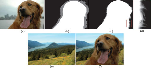
FIGURE 9.1
An image matting example: (a) original image, (b) user specified trimap, where white means foreground, black means background, and gray means unknown, (c) extracted alpha matte, white means higher alpha value, (d) a close-up view of the highlighted region on the alpha matte, (e) a new background image, (f) a new composite.

Matting can be viewed as an extension to the classic binary segmentation problem, where each pixel is assigned fully to either the foreground or the background, i.e., α_p ∈ {0, 1}. In natural images, although the majority of pixels are usually either definite foreground or definite background, accurately estimating fractional alpha values for pixels on the foreground edge is essential for extracting fuzzy object boundaries such as hair or fur, as shown in the example in Figure 9.1.

9.1.1    User Constraint

Matting is inherently an under-constrained problem. Assuming the input image has three color channels, seven unknown variables (three for f_p, three for b_p, and one for α_p) need to be estimated from three color channel values of c_p. Without any additional constraint, the problem is ill-posed and many possible solutions exist. For instance, a simple solution satisfying the Compositing Equation is to set f_p = b_p = c_p, and choose α_p arbitrarily. This is obviously not the correct solution for separating the foreground. In order to estimate an alpha matte that represents the correct foreground coverage, most matting approaches rely on both user guidance and prior knowledge on natural image statistics to constrain the solution space. A typical user constraint provided to a matting system is a trimap, where each pixel in the image is assigned to three possible values: definite foreground $ℱ$ (α_p = 1), definite background $ℬ$ (α_p = 0), and unknown $\mathcal{U}$ (α_p to be determined). Figure 9.1b shows an example of a user-specified trimap. Given the input trimap, the task of matting is thus reduced to estimating alpha values for unknown pixels, under the constraint of the known pixels in $ℱ$ and $ℬ$.

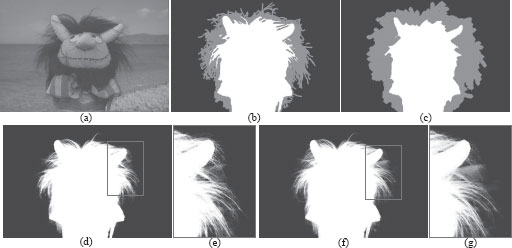
FIGURE 9.2
Image matting with different trimaps: (a) input image, (b) a tight trimap, (c) a coarse trimap, (d) matte generated using the tight trimap, (e) a close-up view of the highlighted region in (d), (f) matte generated using the coarse trimap, (g) a close-up view of the highlighted region in (f). Both mattes are generated using the Robust matting algorithm [2].

The accuracy of the input trimap has a direct impact on the quality of the final alpha matte. In general, an accurately specified trimap, where the unknown region covers only truly semitransparent pixels, often leads to a more accurate alpha matte than a loosely defined trimap, due to the reduced number of unknown variables. An example is shown in Figure 9.2, where the same matting algorithm is applied to the same input image with two different trimaps. The trimap in Figure 9.2b is more accurate than the one shown in Figure 9.2c. Therefore, it leads to a more accurate alpha matte, as shown in Figure 9.2d to Figure 9.2g.

Given that manually specifying an accurate trimap is still a tedious process, fast image segmentation approaches have been adopted in matting systems for efficient trimap generation. The Grabcut system [3] can generate a fairly accurate binary segmentation of the foreground object starting from a user-specified bounding box, using iterated graph cuts optimization. Under a similar optimization framework, the Lazy Snapping system [4] generates a binary segmentation from a few foreground and background scribbles. Once the binary segmentation is obtained, one can simply erode and dilate the foreground contour to create an unknown region for matting. Rhemann et al. [5] proposed a more accurate trimap segmentation tool, which explicitly segments the image into three regions $ℱ$, $ℬ$, and $\mathcal{U}$, using a parametric max-flow algorithm. With the help of these techniques, accurate trimaps can be efficiently generated with a small amount of user interaction.

In this chapter, for image matting, we assume the trimap is already given, and focus on how to estimate fractional alpha values in the $\mathcal{U}$ region. For video matting, we will describe how to generate temporally consistent trimaps for video frames, as it is the main bottleneck for applying matting techniques in video.

9.1.2    Earlier Approaches

Earlier matting approaches try to estimate alpha values for individual pixels independently without any spatial regularization. A common strategy is that for an unknown pixel p, sampling a set of known foreground and background colors nearby as priors for f_p and b_p. Assuming the image colors vary smoothly, these samples can be treated as reasonably accurate estimates of f_p and b_p. Once f_p and b_p are estimated, solving α_p from the composting equation becomes trivial.

Various statistical models have been used to estimate f_p and b_p from color samples. Ruzon and Tomasi developed a parametric sampling algorithm [6], where foreground and background color samples are modeled as mixture of Gaussians, and the observed color c_p is modeled as coming from an intermediate distribution between the foreground and background Gaussian distributions. Mishima [7] developed a blue screen matting system which uses color samples in a nonparametric way. Detailed explanations of these methods can be found in Wang and Cohen’s survey [8].

A notable method among early approaches is the Bayesian matting [9] approach, which formulates the estimation of f_p, b_p, and α_p in a Bayesian framework, and solves the matte using the maximum a posteriori (MAP) technique. It is the first to cast the matting problem into a well-formulated statistical inference framework. Mathematically, for an unknown pixel p, its matting solution is formulated as:

$\arg \underset{f_p,b_p,{\alpha }_p}{\max }P\left(f_p,b_p,{\alpha }_p|c_p\right)=\arg \underset{f_p,b_p,{\alpha }_p}{\max }L\left(c_p|f_p,b_p,{\alpha }_p\right)+L\left(f_p\right)+L\left(b_p\right)+L\left({\alpha }_p\right),$

(9.2)

where L(·) is the log likelihood L(·) = logP(·). The first term on the right side is measured as:

$L\left(c_p|f_p,b_p,{\alpha }_p\right)=-{\Vert c_p-{\alpha }_p{f}_p-\left(1-{\alpha }_p\right)b_p\Vert }^2/{\sigma }_p^2,$

(9.3)

where the color variance σ_p is measured locally. This is simply the fitting error according to the compositing equation. To estimate L(f_p), foreground colors in the nearby region are first partitioned into groups, and in each group an oriented Gaussian is estimated by computing the mean $\overline{f}$ and covariance Σ_F. L(f_p) is then defined as:

$L\left(f_p\right)=-{\left(f_p-\overline{f}\right)}^T{\sum }_F^{-1}\left(f_p-\overline{f}\right)/2.$

(9.4)

L(b_p) is calculated in the same way using background samples. L(α_p) is treated as a constant. The solution of the inference problem is obtained by iteratively estimating (f_p, b_p) and α_p.

Despite their success in simple cases, matting approaches that only depend on color sampling often fail on more complicated images where foreground and background color distributions are overlapping, and the input trimap is loosely defined. This is due to two fundamental limitations of this framework. First, estimating alpha values independently for individual pixels without any spatial regularization is prone to image noise. Second, when the trimap is loosely defined, the sampled foreground and background colors are no longer good priors for estimating f_p and b_p, leading to estimation bias. Modern matting approaches try to avoid these limitations by enforcing local spatial regularization on the estimated alpha matte, which allows them to perform more robustly on difficult examples. We will focus on these methods from now on.

9.2    Graph Construction for Image Matting

Modern image matting approaches usually start by modeling the input image as an undirected and weighted graph $\mathcal{G}=\left(\mathcal{V},ℰ\right)$, where each ${\upsilon }_i\in \mathcal{V}$ corresponds to an unknown pixel, i.e., a pixel in the $\mathcal{U}$ region of the input trimap². An edge $e_i\in ℰ$ is usually defined between a node and its four spatial neighbors, although in some work the edges are defined among pixels in larger spatial neighborhoods such as 3 × 3 or 5 × 5 [10]. Additionally, some approaches define a node weight w_i for each node υ_i, which encodes some prior knowledge of the alpha value of υ_i, given its observed color c_i and nearby foreground and background colors. The structure of such a graph is shown in Figure 9.3. Using this graph representation, matting is transferred into a graph labeling problem, where the objective is to solve for the optimal α_is that can minimize the total energy of the graph.

Although many image matting approaches share the same common graph structure, the key difference among them is the formulation of the edge weight w_ij, and optionally the node weight w_i. Table 9.1 summaries some representative image matting techniques that will be discussed in this section, and their choices of the edge and the node weights. Specifically, different edge weights will be discussed in detail in Section 9.2.1, and various node weights will be illustrated in Section 9.2.2. Finally, how to solve the graph labeling problem using the define edge and node weights will be described in Section 9.3.

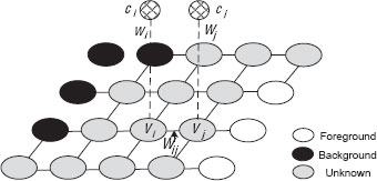
FIGURE 9.3
A typical graph setup for image matting.

Method	Reference	Edge weight	Node weight	Optimization method
Random walk matting	[11]	$w_{ij}^{\text{lpp}}$ (Eqn.9.7)	No	Linear system
Easy matting	[12]	$w_{ij}^{\text{easy}}$ (Eqn.9.8)	$w_i^{\text{easy}}$ (Eqn.9.21)	Linear system
Iterative BP matting	[13]	$w_{ij}^{\text{bp}}$ (Eqn.9.9)	$w_i^{\text{bp}}$ (Eqn.9.22)	Belief propagation
Closed-form matting	[10]	$w_{ij}^{\text{cf}}$ (Eqn.9.13)	No	Linear system
Robust matting	[2]	$w_{ij}^{\text{cf}}$ (Eqn.9.13)	$w_i^{\text{rm}}$ (Eqn.9.27)	Linear system
Learning-based matting	[14]	$w_{ij}^{\ln }$ (Eqn.9.20)	No	Linear system
Global sampling matting	[15]	$w_{ij}^{\text{cf}}$ (Eqn.9.13)	$w_i^{\text{gs}}$ (Eqn.9.32)	Linear system

TABLE 9.1
Summary of image matting techniques and their graph structures.

9.2.1    Defining Edge Weight w_ij

One straightforward idea of mapping pixel colors to the edge weight e_ij is to use the following classic Euclidean norm:

$w_{ij}=\exp \left(-\frac{{\Vert c_i-c_j\Vert }^2}{{\sigma }_{ij}^2}\right),$

(9.5)

where c_i is the RGB color of υ_i, σ_ij is a parameter which can be either manually selected by the user, or automatically computed based on local image statistics [16]. This function penalizes large alpha changes in flat image regions where the color difference between two neighboring pixels is small. This metric has been widely used in graph-based binary image segmentation systems [17]. Grady et al. [11] adopted this formulation for image matting, but instead of measuring the Euclidean norm in the RGB color space, they proposed to use the Locality Preserving Projections (LPP) technique [18] to define a conjugate norm, which is more reliable for describing perceptual object boundaries than the RGB color space. Mathematically, the projections defined by the LPP algorithm are given by solving the following generalized eigen-vector problem:

$ZL{Z}^{T}x=\lambda ZD{Z}^{T}x,$

(9.6)

where Z is a 3 × N (the number of pixels in the image) matrix with each c_i color vector as a column, D is the diagonal matrix defined as $D_{ii}=d_i\dot{=}\sum w_{ij}$, and L is the sparse Laplacian matrix where L_ii = d_i, and L_ij = −w_ij for j ≠ i. Denote its solution by Q where each eigenvector is a row, the final edge weight is computed as:

$w_{ij}^{\text{lpp}}=\exp \left(-\frac{{\left(c_i-c_j\right)}^T{Q}^{T}Q\left(c_i-c_j\right)}{{\sigma }_{ij}^2}\right).$

(9.7)

The edge weights defined above are static given an input image, and they are not related to the values of the random variables α_i and α_j. In some other approaches, the edge weight is explicitly defined as a function of α_i and α_j to enforce the alpha matte to be locally smooth. The Easy matting system [12] defines the edge weight in a quadratic form as:

$w_{ij}^{\text{easy}}=\lambda \cdot \frac{{\left({\alpha }_i-{\alpha }_j\right)}^2}{\Vert c_i-c_j\Vert },$

(9.8)

where λ is a user defined constant. Minimizing the sum of edge weights over the graph will force the alpha values of adjacent pixels to be similar if local image gradient is small. Under the same motivation, Wang and Cohen [13] constructed a Markov Random Field (MRF) where the joint distribution over α_i and α_j is given by the Boltzmann distribution of a similar quadratic energy function as:

$w_{ij}^{\text{bp}}=\exp \left(-\frac{{\left({\alpha }_i-{\alpha }_j\right)}^2}{{\sigma }_{\text{const}}^2}\right).$

(9.9)

All the edge weights defined above implicitly assume that the input image is locally smooth. In the closed-form matting algorithm [10], the local smoothness is explicitly modeled using a color line model. That is, in a small local window ϒ (3 × 3 or 5 × 5), the foreground and background colors (f_is and b_is) are linear mixtures of two latent colors:

$\begin{array}{ccc}{f}_i={\beta }_i^f{f}_{l1}+\left(1-{\beta }_i^f\right)f_{l2}& \text{and}& b_i={\beta }_i^b{b}_{l1}\end{array}+\left(1-{\beta }_i^b\right)b_{l2},\forall i\in \Upsilon ,$

(9.10)

where f_l1, f_l2, b_l1, and b_l2 are latent colors. Combining this constraint with the Compositing Equation, it is easy to show that alpha values in ϒ can be expressed as:

${\alpha }_i={\displaystyle \sum _k{a}^k{c}_i^k+b,\forall i}\in \Upsilon ,$

(9.11)

where k refers to color channels, and a^k and b are functions of ${\beta }_i^f,{\beta }_i^b$, f_l1, f_l2, b_l1 and b_l2, thus they are constants in the window. Based on this constraint, Levin et al. [10] defined a quadratic matting cost function as:

$J\left(\alpha ,a,b\right)={\displaystyle \sum _{j\in I}\left({\displaystyle \sum _{i\in {\Upsilon }_j}{\left({\alpha }_i-{\displaystyle \sum _k{a}_j^k{c}_i^k-b_j}\right)}^2}+ϵ{\displaystyle \sum _k{a}_j^{k2}}\right)},$

(9.12)

where the second term is a regularization term mainly for the purpose ot numerical stability. It also has a desirable side effect of biasing the solution toward smoother alpha mattes, since a_j = 0 means that α is constant over the jth window. Given this cost function, the edge weight can be derived as:

$w_{ij}^{\text{cf}}=\frac{1}{\left|{\Upsilon }_k\right|}{\displaystyle \sum _{k|\left(i,j\right)\in {\Upsilon }_k}\left(1+{\left(c_i-{\mu }_k\right)}^T{\left({\displaystyle {\sum }_k+}\frac{\epsilon }{\left|{\Upsilon }_k\right|}{I}_3\right)}^{-1}\left(c_j-{\mu }_k\right)\right)},$

(9.13)

where Σ_k is a 3 × 3 covariance matrix, μ_k is a 3 × 1 mean vector of the colors in the window ϒ_k, and I₃ is the 3 × 3 identity matrix. Consequently, a graph Laplacian matrix can be computed as:

$L_{ij}^{\text{cf}}=\{\begin{array}{lll}-w_{ij}^{\text{cf}}\hfill & :\hfill & \text{if}i\ne j,\left(i,j\right)\in {\Upsilon }_k,\hfill \\ {\displaystyle {\sum }_{l,l\ne i}{w}_{il}^{\text{cf}}}\hfill & :\hfill & \text{if}i=j,\hfill \\ 0\hfill & :\hfill & \text{otherwise}\text{.}\hfill \end{array}$

(9.14)

which is called the matting Laplacian. It is easy to show that the Laplacian matrix L^cf is symmetric and positive semidefinite.

There are several unique characteristics of the edge weight $w_{ij}^{\text{cf}}$. First, each pixel has a nonzero weight with all other pixels in a local (5 × 5 if ϒ is 3 × 3) neighborhood, thus the Laplacian matrix is a much denser one than that of a typical four-neighbor image graph. In each row of the Laplacian matrix L^cf, there are 25 nonzero elements, compared with 5 in a four-neighbor graph Laplacian. Second, the edge weight $w_{ij}^{\text{cf}}$ can be negative, which is different from the strictly nonnegative edge weights defined in Equation 9.5 to 9.9. It is thus worth emphasizing that some of the commonly used nonnegative graph analysis methods do not apply to L^cf. For instance, in a nonnegative graph, the degree of a vertex υ_i is d_i = Σ w_ij for all edges e_ij incident on υ_i, and is often used for normalizing all nonzero values in the ith row of the graph Laplacian [17]. For the matting Laplacian L^cf, computing the degree of a vertex and using it for normalization is no longer suitable, as positive and negative values cancel out each other. Another side effect of using negative edge weights is that the computed alpha values are no longer guaranteed to be within [0, 1], as discussed in [19]. Using this method it is quite often to get alpha values that are out of bounds, thus in practice one has to clip the alpha values at 0 and 1 to generate visually correct alpha mattes.

Since the matting Laplacian L^cf is strictly derived from the color line model, it otten leads to accurate alpha mattes when the underlying color model is satisfied. In practice, if the input image is composed of smooth regions without strong textures, the color line model often holds true. Given its generality and accuracy, it has been widely used in recent matting approaches where it is combined with other techniques to achieve high-quality results. It has also been applied in many other applications such as image dehazing [20] and light source separation [21] as a general edge-aware interpolation tool.

The limitations of the matting Laplacian L^cf have also been extensively studied. Singaraju et al. [22] demonstrated that the color line model provides an overfit and leads to ambiguity when the intensity variations of the foreground and background layers are much simpler than the color line. Specifically, they studied two compact color models, point-point color model and line-point color model. The former applies when both the foreground and background intensities are locally constant (the point constraint), and the latter applies when one layer satisfies the point constraint while the other satisfies the color line constraint. These two color models lead to modified edge weights which work better than the original matting Laplacian in these special cases.

To deal with more complicated cases where a linear color model is incapable of accurately describing the color variations, Zheng et al. [14] proposed a semisupervised learning approach, where the well-known kernel trick [23] is used to deal with nonlinear local color distributions. This approach assumes that the alpha value of an unknown pixel υ_i is a linear combination of the alpha values of its neighboring pixels, e.g., a 7 × 7 window centered at the pixel:

${\alpha }_i={\xi }_i^T\alpha ,$

(9.15)

where α is the alpha value vector of all pixels in the image, and ξ_i is a coefficient vector where the majority values are 0 except for pixels which are in the neighborhood of υ_i. By introducing a new matrix G through stacking ξ_is: G = [ξ₁, …, ξ_n], the above equation can be rewritten as:

$\alpha =G^T\alpha .$

(9.16)

This leads to a solution of α by minimizing the following quadratic cost function:

$\arg \underset{\alpha }{\min }{\Vert \alpha -G^T\alpha \Vert }^2,$

(9.17)

which can be reformulated as:

$E^{\ln }\left(\alpha \right)={\alpha }^T\left(I_n-G\right){\left(I_n-G\right)}^T\alpha .$

(9.18)

The Laplacian matrix of this approach is then defined as:

$L^{\ln }=\left(I_n-G\right){\left(I_n-G\right)}^T,$

(9.19)

and the corresponding edge weight is

$w_{ij}^{\ln }=L^{\ln }\left(i,j\right).$

(9.20)

The matrix G is obtained by training a non-linear alpha-color model from known pixels in the trimap, either locally or globally, as detailed in the original paper [14].

9.2.2    Defining Node Weight w_i

For each υ_i, the node weight w_i measures how compatible an estimated α_i is with its observed color c_i, and nearby foreground and background colors. Not all matting approaches define and use this term, but it has been shown [2] that the node weight, if defined properly, can lead to more accurate alpha estimation.

A common approach for defining w_i is to first sample a set of nearby known foreground and background colors, denoted as $c_k^f$ and $c_l^b$, 0 < k, l < N, as shown in Figure 9.4. Assuming the foreground and background colors vary smoothly, these color samples assemble reasonable probabilistic distributions of f_i and b_i. Combined with c_i, these samples can be used to test the feasibility of an estimated α_i using the compositing equation. Using this idea, Guan et al. [12] defined the node weight in the Easy Matting system as:

$w_i^{\text{easy}}=\frac{1}{N^2}{\displaystyle \sum _{k=1}^N{\displaystyle \sum _{l=1}^N{\Vert c_i-{\alpha }_i{c}_k^f-\left(1-{\alpha }_i\right)c_l^b\Vert }^2/{\sigma }_i^2}},$

(9.21)

where σ_i is the distance variance among c_i and ${\alpha }_i{c}_k^f+\left(1-{\alpha }_i\right)c_l^b$. This node weight favors an α_i that can best explain the observed color c_i as a linear combination of the sampled colors $c_k^f$ and $c_l^b$. Similarly, Wang and Cohen [13] defined a node weight using exponential functions as:

$w_i^{\text{bp}}=\frac{1}{N^2}{\displaystyle \sum _{k=1}^N{\displaystyle \sum _{l=1}^N{\mu }_k^f{\mu }_l^b}}\cdot \exp \left(-{\Vert c_i-{\alpha }_i{c}_k^f-\left(1-{\alpha }_i\right)c_l^b\Vert }^2/{\sigma }_i^2\right),$

(9.22)

where ${\mu }_k^f$ and ${\mu }_l^b$ are additional weights for color samples based on their spatial distances to υ_i.

The node weights defined in Equation 9.21 and 9.22 treat every color sample equally. In practice, however, when the size of the sample set is large and the foreground and background color distributions are complex, the samples set may present a large color variance. It is often the case that only a small number of samples are good for estimating α_i. To decide which samples are good for defining w_i, Wang and Cohen [2] proposed a color sample selection method. In this approach, “good” sample pairs are defined as those that can explain c_i as a convex combination of themselves. Mathematically, as illustrated in Figure 9.4, for a pair of foreground and background colors $\left(c_k^f,c_l^b\right)$, a distance ratio is defined as:

$R_d\left(c_k^f,c_l^b\right)=\frac{\Vert c_i-{\widehat{\alpha }}_i{c}_k^f-\left(1-{\widehat{\alpha }}_i\right)c_l^b\Vert }{\Vert c_k^f-c_l^b\Vert },$

(9.23)

where ${\widehat{\alpha }}_i$ is the alpha value estimated from this sample pair as:

${\widehat{\alpha }}_i=\frac{\left(c_i-c_l^b\right)\left(c_k^f-c_l^b\right)}{{\Vert c_k^f-c_l^b\Vert }^2}.$

(9.24)

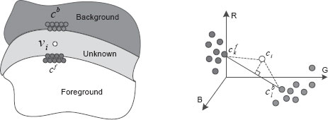
FIGURE 9.4
Left: to define the node weight for an unknown pixel υ_i, a set of spatially nearby foreground and background colors c^f and c^b are collected. Right: a sample pair $c_k^f$ and $c_l^b$ is considered to be a good estimation of the true foreground and background colors of υ_i if $c_k^f$, $c_l^b$, and c_i together satisfy the linear constraint in the RGB color space.

$R_d\left(c_k^f,c_l^b\right)$ essentially measures the linearity of $c_k^f,c_l^b$, and I_i in the color space. It is easy to show that $R_d\left(c_k^f,c_l^b\right)$ is small if the three colors approximately lie on a color line, and vise versa. Based on the distance ratio, a confidence value for the sample pair is defined as:

$f\left(c_k^f,c_l^b\right)=\exp \left(-\frac{R_d\left(c_k^f,c_l^b\right)}{{\sigma }_c^2}\right)\cdot \gamma \left(c_k^f\right)\cdot \gamma \left(c_l^b\right),$

(9.25)

where σ_c is a constant set at 0.1. $\gamma \left(c_k^f\right)$ is the weight for the color $c_k^f$:

$\gamma \left(c_k^f\right)=\exp \left(-\frac{{\Vert c_k^f-c_i\Vert }^2}{{\min }_k\left({\Vert c_k^f-c_i\Vert }^2\right)}\right),$

(9.26)

which favors foreground samples that are close to the target pixel. $\gamma \left(c_l^b\right)$ is defined in a similar way.

Given a set of foreground and background samples, this approach exhaustively examines every possible foreground background sample combination, and finally chooses a few sample pairs (typically 3) with the highest confidence values. Denote the average confidence value of these pairs as ${\overline{f}}_i$, and the average alpha value estimated from these pairs using Equation 9.24 as ${\overline{\alpha }}_i$, the final node weight is computed as

$w_i^{\text{rm}}={\overline{f}}_i\cdot {\left({\alpha }_i-{\overline{\alpha }}_i\right)}^2+\left(1-{\overline{f}}_i\right){\left({\alpha }_i-H\left({\overline{\alpha }}_i-0.5\right)\right)}^2,$

(9.27)

where H(x) is the Heaviside step function which outputs 1 when x > 0 and 0 otherwise. This node weight encourages the final alpha value α_i to be close to ${\overline{\alpha }}_i$ when the sampling confidence ${\overline{f}}_i$ is high, and α_i to be either 0 or 1 when the confidence is low. When the confidence is low, it suggests that c_i cannot be well approximated as a linear interpolation of known foreground and background colors, and it is thus more likely to be a new foreground or background color.

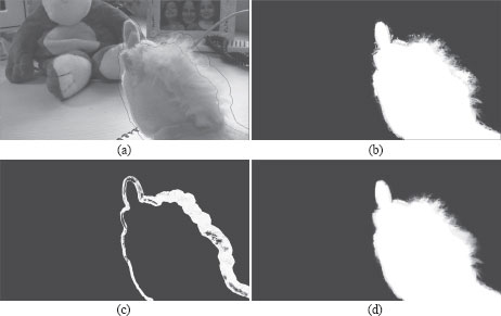
FIGURE 9.5
An example of the color sampling method used in the Robust Matting system [2]. (a) Input image with overlayed trimap, (b) initial alpha matte computed by Equation 9.24 using best sample pairs, (c) the confidence map computed by Equation 9.25, white means higher confidence values, (d) final alpha matte after minimizing the energy in Equation 9.40.

Figure 9.5 shows an example of using this sampling method for alpha matting. Given the input image and the specified trimap as shown in Figure 9.5a, the alpha matte ${\overline{\alpha }}_i$ computed using Equation 9.24, and the confidence map ${\overline{f}}_i$ computed using Equation 9.25 are visualized in Figure 9.5b and 9.5c. The final alpha matte of the Robust Matting algorithm after minimizing the energy function in Equation 9.40 is shown in Figure 9.5d.

Based on the color sampling method described above, Rhemann et al. [24] proposed an improved sampling procedure for defining the node weight. In Wang and Cohen’s work, foreground and background samples are selected solely based on their spatial distances to υ_i, without considering the underlying image structures. To improve this, Rhemann et al. proposed to select foreground samples based on their geodesic distances [25] to υ_i in the image space. This distance measure encourages the foreground samples to not only be close to υ_i spatially, but also belong to the same connected image component as υ_i. In this approach, a confidence function that is slightly different from Equation 9.25 is defined as:

$f_2\left(c_k^f,c_l^b\right)=\exp \left(-\frac{R_d\left(c_k^f,c_l^b\right)\cdot {\gamma }^{\prime }\left(c_k^f\right)\cdot {\gamma }^{\prime }\left(c_l^b\right)}{{\sigma }_c^2}\right),$

(9.28)

where the sample weights are defined as

$\{\begin{array}{cc}{\gamma }^{\prime }\left(c_k^f\right)& =\exp \left(-\frac{{\max }_k\left({\Vert c_k^f-c_i\Vert }^2\right)}{{\Vert c_k^f-c_i\Vert }^2}\right),\\ {\gamma }^{\prime }\left(c_l^b\right)& =\exp \left(-\frac{{\max }_k\left({\Vert c_l^b-c_i\Vert }^2\right)}{{\Vert c_l^b-c_i\Vert }^2}\right).\end{array}$

(9.29)

Both sampling procedures described above exhaustively examine every possible combination of foreground and background samples, thus their computational cost is high. For instance, if N (N = 20 in [2]) samples are collected for both the foreground and the background, N² pair evaluations have to be performed for every unknown pixel. To reduce the computational cost while maintaining the sampling accuracy, Gastal and Oliveira proposed a Shared Sampling method [26], which is motivated by the fact that pixels in a small neighborhood usually share the same attributes. This algorithm first selects at most k_g (a small number) foreground and background samples for each pixel, resulting in at most $k_g^2$ test pairs, from which the best pair is selected. The algorithm also makes sure that sample sets of neighboring pixels are disjoint. Then, in a small neighborhood of k_r pixels, each pixel analyzes the best choices of its k_r spatial neighbors, and chooses the best sample pair as its final decision. Thus, while in practice $k_g^2+k_r$ pair evaluations are performed for each pixel, due to the affinity among neighboring pixels, this is roughly equivalent to performing $k_g^2\times k_r$ pair evaluations. In their system, k_g and k_r are set to be 4 and 200, respectively, thus 4 × 4 + 200 = 216 pair evaluations can achieve the effect of evaluating 16 × 200 = 3200 pairs. Using this efficient sampling method plus some local smoothing postprocessing steps, Gastal and Oliveira developed a real-time matting system which achieves high accuracy on the publicly available online matting benchmark [27].

The sampling procedures described so far are all local sampling methods, i.e., for an unknown pixel, only a limited number of nearby foreground and background colors are collected for alpha estimation. He et al. [15] pointed out that due to the limited size of the sample set and sometimes complex foreground structures, local sampling may not always cover the true foreground and background colors of unknown pixels. They further proposed a global sampling approach, where for evaluating the alpha value of an unknown pixel, all known foreground and background colors in the image are used as samples. Specifically, from all possible sample pairs, the best one is chosen which minimizes the cost function:

$E^{\text{gs}}\left(c_k^f,c_l^b\right)=\kappa \Vert c_i-{\widehat{\alpha }}_i{c}_k^f-\left(1-{\widehat{\alpha }}_i\right)c_l^b\Vert +\eta \left(x_k^f\right)+\eta \left(x_l^b\right),$

(9.30)

where ${\widehat{\alpha }}_i$ is the alpha value estimated from $c_k^f$ and $c_l^b$ using Equation 9.24, κ is a balancing weight and $\eta \left(x_k^f\right)$ is the spatial energy computed from the spatial location of $c_k^f$ and c_i as:

$\eta \left(x_k^f\right)=\frac{\Vert x_k^f-x_i\Vert }{{\min }_k\Vert x_k^f-x_i\Vert }.$

(9.31)

$\eta \left(x_l^b\right)$ is the spatial energy computed for $c_l^b$ in the same way. To handle the computational complexity introduced by the large number of samples, their system poses the sampling task as a correspondence problem in a special “FB search space”, and uses a generalized fast patch matching algorithm [28] to efficiently find the best sample pair in that space, denoted as ${\widehat{c}}_k^f$ and ${\widehat{c}}_l^b$. After sample search, the node weight is finally defined as:

$w_i^{\text{gs}}=\exp \left(-\left|c_i-{\widehat{\alpha }}_i{c}_k^f-\left(1-{\widehat{\alpha }}_i\right)c_l^b\right||\right){\left({\alpha }_i-{\widehat{\alpha }}_i\right)}^2.$

(9.32)

Note that the global sampling method intrinsically assumes that the foreground and background color distributions are spatially invariant, so that the color samples that are spatially far away from the target pixel may still be valid estimations of the true foreground and background colors of the pixel. If the foreground or background colors are spatially varying, using remote color samples may introduce additional color ambiguity which will lead to less accurate alpha estimation.

9.3    Solving Image Matting Graphs

Once the edge and node weights are properly defined for the matting graph, solving the alpha matte becomes a graph labeling problem. Depending on exactly how the edge and node weights are formulated, various optimization techniques can be applied to obtain the solution. Here we review a few representative techniques that have been widely used in existing matting systems.

9.3.1    Solving MRF

Wang and Cohen proposed an iterative optimization approach [13] to compute the alpha matte from sparsely specified user scribbles. In this method, the matting graph is formulated as a Markov Random Field (MRF), and the total energy to be minimized is defined as:

$E^{\text{bp}}\left(\alpha \right)={\displaystyle \sum _{{\upsilon }_i\in \mathcal{V}}{w}_i^{\text{bp}}+\lambda .{\displaystyle \sum _{{\upsilon }_i,{\upsilon }_j\in \mathcal{V}}{w}_i^{\text{bp}},}}$

(9.33)

where $w_i^{\text{bp}}$ is the node weight defined in Equation 9.22, and $w_{ij}^{\text{bp}}$ is the edge weight in Equation 9.9. This approach also quantizes the continuous alpha value in [0, 1] into multiple discrete levels so that discrete optimization is applicable. With the MRF defined in this way, finding alpha labels corresponds to the MAP estimation problem, which can be practically solved using the loopy Belief Propagation (BP) algorithm [29].

To generate accurate alpha mattes from sparsely defined user trimaps, in this approach the energy minimization method described above is applied iteratively in an active region. The active region is created and updated iteratively by expanding the user scribbles toward the rest of the image until all unknown pixels have been covered. This ensures that pixels nearby the user scribbles are computed first, and they will in turn affect other pixels that are far away from the scribbles. In each iteration of the algorithm, the data weight $w_i^{\text{bp}}$ and edge weight $w_{ij}^{\text{bp}}$ are updated based on the alpha matte computed in the previous iteration, and a new energy E^bp(α) is minimized using the BP algorithm.

9.3.2    Linear Optimization

One of the major limitations of the MRF formulation is its high computational complexity. Furthermore, iteratively applying the BP optimization may lead the algorithm to converge to a local minimum. To avoid these limitations, some approaches carefully define their energy functions in such a way that they can be efficiently solved by closed-form optimization techniques.

Grady et al. [11] defined a matting graph where the edge weight $w_{ij}^{\text{lpp}}$ is formulated as Equation 9.7, and solved the graph labeling problem using Random Walks. In this algorithm, α_i is modeled as the probability that a random walker starting from v_i will reach a pixel in the foreground before striking a pixel in the background, when biased to avoid crossing the foreground boundary. Denote the degree of υ_i as:

$d_i^{\text{rm}}={\displaystyle \sum w_{ij}^{\text{lpp}}},$

(9.34)

for all edges e_ij incident on υ_i. The probability that a random walker at υ_i transitions to υ_j is computed as $p_{ij}=w_{ij}^{\text{lpp}}/d_i$. Theoretical studies [30] show that the solution to the random walker problem is exactly the solution to the inhomogeneous Dirichlet problem from potential theory, given Dirichlet boundary conditions that α_j = 1 if υ_j is in the foreground region of the trimap, and α_j =0 if υ_j is in the background region. Specifically, these probabilities are an exact, steady-state, global minimum to the Dirichlet energy functional:

$E^{\text{rm}}\left(\mathbf{\alpha }\right)={\mathbf{\alpha }}^T{L}^{\text{rm}}\mathbf{\alpha },$

(9.35)

subject to the boundary conditions. L^rm is the graph Laplacian given by:

$L_{ij}^{\text{rm}}=\{\begin{array}{ll}{d}_i^{\text{rm}}\hfill & :\text{if}i=j,\hfill \\ -w_{ij}^{\text{lpp}}\hfill & \text{:}\text{if i and j are neighbors,}\hfill \\ 0\hfill & :\text{otherwise}\text{.}\hfill \end{array}$

(9.36)

The energy functional in Equation 9.35 can be efficiently minimized by solving a sparse, symmetric, positive-definite linear system, and has been further implemented on GPU for real-time interaction [11].

Similar to Wang and Cohen’s approach [13], the Easy Matting system [12] also employs an iterative optimization framework. In the kth iteration, the total energy to be minimized is defined as

$E^{\text{easy}}\left(\alpha ,k\right)={\displaystyle \sum _{{\upsilon }_i\in \mathcal{V}}{w}_i^{\text{easy}}+{\lambda }_k}\cdot {\displaystyle \sum _{{\upsilon }_i,{\upsilon }_j\in \mathcal{V}}{w}_{ij}^{\text{easy}}},$

(9.37)

where $w_i^{\text{easy}}$ is the node weight defined in Equation 9.21, and $w_i^{\text{easy}}$ is the edge weight defined in Equation 9.8. Note that since both terms are carefully defined in quadratic forms, this energy function can be efficiently minimized by solving a large linear system. Also, unlike E^bp(α) defined in Equation 9.33 which uses a constant weight λ for balancing the two energy terms, the weight λ_k in Equation 9.37 is dynamically adjusted as

${\lambda }_k=e^{-{\left(k-\beta \right)}^3},$

(9.38)

where k is the number of iterations, and β is a predefined constant which is set to be 3.4 in the system. In this setting, λ_k becomes smaller when the iteration number k increases. This allows the foreground and background regions to grow faster from sparsely specified user scribbles in early iterations, by using large λ_k values early on. In later iterations when the foreground and background regions encounter, a smaller λ_k will allow the node weight $w_i^{\text{easy}}$ to play a bigger role on determining alpha values for pixels on the foreground edge.

Based on the edge weight defined in Equation 9.13, Levin et al. proposed a matting energy as:

$E^{\text{cf}}\left(\alpha \right)={\alpha }^T{L}^{\text{cf}}\alpha ,$

(9.39)

where L^cf is the matting Laplacian defined in Equation 9.14. This is again a problem of minimizing a quadratic error score, which can be solved as a linear system. Built upon this, the Robust Matting algorithm [2] defines its energy function as:

$E^{\text{rm}}\left(\alpha \right)={\displaystyle \sum _{{\upsilon }_i\in \mathcal{V}}{w}_i^{\text{rm}}+\lambda \cdot {\alpha }^T{L}^{\text{cf}}\alpha ,}$

(9.40)

where $w_i^{\text{rm}}$ is the node weight defined in Equation 9.27. The shared matting approach [26] and the global sampling approach [15] minimize a similar energy function, except that the node weight w_i is determined using the shared sampling approach or the global sampling approach described in Section 9.2.2.

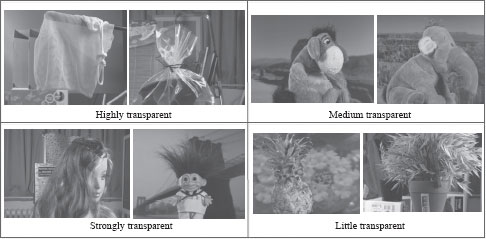
FIGURE 9.6
The height test images with different properties in the online image matting benchmark [27].

9.4    Data Set

To quantitatively compare various image matting approaches, Rhemann et al. [27] proposed the first online benchmark³ for image matting. This benchmark provides a high resolution ground truth data set, which contains 8 test and 27 training images, along with predefined trimaps. These images were shot in a controlled environment, and the ground truth mattes were extracted using the triangulation method [31], by shooting the same foreground object against multiple single-colored backgrounds. The test images have different properties such as hard and soft boundaries, translucency, or different boundary topologies, as shown in Figure 9.6.

3  ³The web URL for the benchmark is www.alphamatting.com.

The online system also provides all scripts and data necessary to allow people to submit new results on the test images, and compare them with results of other approaches in the system. Four different error metrics have been implemented when comparing results to the ground truth: absolute differences (SAD), mean squared error (MSE), and two other perceptually motivated measures named as connectivity and gradient errors. Since introduced, this benchmark has been used by many recent image matting systems for objective and quantitative evaluation.

9.5    Video Matting

9.5.1    Overview

Video matting refers to the problem of estimating alpha mattes of dynamic foreground objects from a video sequence. Compared with image matting, it is a considerably harder problem due to two new challenges: interaction efficiency and temporal coherence.

In image matting systems, the user is usually required to manually specify an accurate trimap in order to achieve accurate mattes. However, this quickly becomes tedious for video, as a short video sequence may contain hundreds or thousands of frames, and manually specifying a trimap for each frame requires simply too much work. To minimize the required user interaction, video matting approaches typically ask the user to provide trimaps only on sparsely distributed keyframes, and then use automatic methods to propagate trimaps to other frames. Automatic trimap generation thus becomes the key component of a video matting system.

In the video matting task, in addition to be accurate on each frame, the alpha mattes computed in consecutive frames are required to be temporally coherent. In fact, temporal coherence is often more important than single frame accuracy, as the human visualization system (HVS) is very sensitive to temporal inconsistency presented in a video sequence [32]. Simply applying image matting techniques frame-by-frame without considering temporal coherence often results in temporally jittering alpha mattes. Maintaining temporal coherence of the resulting mattes thus becomes another fundamental requirement for video matting.

9.5.2    Graph-Based Trimap Generation

Video matting approaches usually apply binary foreground object segmentation for trimap generation. Once a binary segmentation is obtained on each frame, the unknown region of the trimap can be easily generated by dilating and eroding the foreground region. An example is shown in Figure 9.9, where for the input image Figure 9.9b, a binary segmentation in Figure 9.9b is first created, which leads to the trimap shown in Figure 9.9c.

In the video object cut-and-paste system [33], each video frame is at first automatically segmented into atomic regions using the watershed image segmentation algorithm [34], mainly for improving the computational efficiency. These atomic regions are treated as basic elements for graph construction. The user is then required to provide accurate foreground object segmentation on a few keyframes as initial guidance, by using existing interactive image segmentation tools. Between each pair of successive keyframes, a 3D graph $\mathcal{G}=\left(\mathcal{V},ℰ\right)$ is then built on atomic regions, as shown in Figure 9.7.

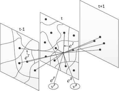
FIGURE 9.7
Graph construction for trimap generation in the video object cut-and-paste system [33].

In graph $\mathcal{G}$, the node set $\mathcal{V}$ includes all atomic regions on all frames between the two keyframes. There are also two virtual nodes υ_F and υ_B, which correspond to definite foreground $ℱ$ and definite background $ℬ$ as hard constraints. There are three types of edges in the graph: intraframe edges e^I, interframe edges e^T, and edges between atomic regions and virtual nodes e^F and e^B. An intraframe edge $e_{ij}^I$ connects two adjacent atomic regions ${\upsilon }_i^t$ and ${\upsilon }_j^t$ on frame t, while an interframe edge $e_{ij}^T$ connects ${\upsilon }_i^t$ and ${\upsilon }_j^{t+1}$, if the two regions have both similar colors and overlapping spatial locations. Every atomic region connects to the virtual nodes υ^F and υ^B.

For edges $e_i^F$ and $e_i^B$, the weights $w_i^F$ and $w_i^B$ encode the user-provided hard constraints, as well as the color similarity between υ_i and user-marked regions. Mathematically, they are defined as:

$w_i^F=\{\begin{array}{lll}0\hfill & :\hfill & \text{if}{\upsilon }_i\in ℱ,\hfill \\ \infty \hfill & :\hfill & \text{if}{\upsilon }_i\in ℬ,\hfill \\ d^F\left({\upsilon }_i\right)\hfill & :\hfill & \text{otherwise;}\hfill \end{array}$

(9.41)

and

$w_i^B=\{\begin{array}{lll}\infty \hfill & :\hfill & \text{if}{\upsilon }_i\in ℱ,\hfill \\ 0\hfill & :\hfill & \text{if}{\upsilon }_i\in ℬ,\hfill \\ d^B\left({\upsilon }_i\right)\hfill & :\hfill & \text{otherwise}\text{.}\hfill \end{array}$

(9.42)

If υ_i is marked as either $ℱ\left({\alpha }_i=1\right)$ or $ℬ\left({\alpha }_i=0\right)$ on the keyframes, then the edge weight is 0 to the corresponding node and ∞ to the other. Otherwise, $w_i^F$ and $w_i^B$ are determined by its color distances to the known foreground and background colors, denoted as d^F (υ_i) and d^B (υ_i). To compute the color distance, Gaussian Mixture Models (GMMs) [35] are used to describe the foreground and background color distributions, collected from the ground-truth segmentations on keyframes. Denote the kth component of the foreground GMM as $\left(w_k^f,{\mu }_k^f,{\sum }_k^f\right)$, representing the weight, the mean color, and the color covariance matrix, respectively, for a given color c, d^F(c) is computed as:

$d^F\left(c\right)=\underset{k}{\min }\left[\widehat{D}\left(w_k^f,{\sum }_k^f\right)+\overline{D}\left(c,{\mathit{\mu }}_k^f,{\sum }_k^f\right)\right],$

(9.43)

where

$\widehat{D}\left(w,\sum \right)=-\log w+\frac{1}{2}\log det\sum ,$

(9.44)

and

$\overline{D}\left(c,\mathit{\mu },\sum \right)=\frac{1}{2}{\left(c-\mu \right)}^T{\sum }^{-1}\left(c-\mu \right).$

(9.45)

For the node υ_i (note that υ_i is an atomic region containing many pixels), its distance to the foreground GMMs d^F(υ_i) is defined as the average distance of d^F (c_j ∈ υ_i), where c_j is the color of a pixel inside the atomic region. The background distance d^F(υ_i) is defined in the same way using the background GMMs.

For the intraframe and interframe edges e^I and e^T, the edge weights are defined as

$w_{ij}=\left|{\alpha }_i-{\alpha }_j\right|\cdot \exp \left(-\beta {\Vert {\overline{c}}_i-{\overline{c}}_j\Vert }^2\right),$

(9.46)

where α_i and α_j are labels for υ_i and υ_j, which are constrained to be either 0 or 1 for the purpose of binary segmentation. β is a parameter that weights the color contrast, which can be set as a constant or computed adaptively using the robust method proposed by Blake et al. [36]. ${\overline{c}}_i$ and ${\overline{c}}_j$ are the average colors of pixels inside υ_i and υ_j.

The total energy to be minimized for the graph labeling problem is

$E\left(\mathit{\alpha }\right)={\displaystyle \sum _{{\upsilon }_i\in \mathcal{V}}\left({\alpha }_i{w}_i^F\right)+\left(1-{\alpha }_i\right)w_i^B}+{\lambda }_1{\displaystyle \sum _{e_{ij}\in e^I}{w}_{ij}}+{\lambda }_2{\displaystyle \sum _{e_{ij}\in e^T}{w}_{ij}},$

(9.47)

where α_i can only be 0 or 1 in this binary labeling problem, and λ₁ and λ₂ are used to adjust the weights of the energy terms. For instance, a higher λ₂ will enforce the solution to be more temporally coherent. This energy function can be minimized using the graph cuts algorithm [16].

After the graph labeling problem is solved, a local tracking and refinement step is further employed to improve the segmentation accuracy. Finally, a trimap is created for each frame by dilating and eroding the segmented foreground region, and a coherent matting approach [37], which is a variant of the Bayesian matting algorithm [9], is used to generate the final alpha mattes. Wang et al. [38] introduced another 3D graph labeling approach for trimap generation in video. Their system first applies the 2D mean shift image segmentation algorithm [39] on each frame to generate oversegmented regions, similar to the atomic regions in the video object cut-and-paste system. The system then treats the 2D mean shift regions as super-pixels by representing each region using the mean position and color of all pixels inside it, and applies the mean shift algorithm again to group 2D regions into 3D spatiotemporal regions. This two-step clustering method results in a strict hierarchical structure of the input video, shown in Figure 9.8a, where each pixel belongs to a 2D region, and each 2D region belongs to a 3D spatiotemporal region.

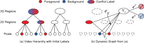
FIGURE 9.8
Video hierarchy and dynamic graph construction in the 3D video cutout system [38]. (a). Video hierarchy created by two-step mean shift segmentation. User-specified labels are then propagated upward from the bottom level. (b). A graph is dynamically constructed based on the current configuration of the labels. Only highest level nodes that have no conflict are selected. Each node in the hierarchy also connects to two virtual nodes υ^F and υ^B.

A unique characteristic of Wang et al.’s system is the dynamic graph construction. In this approach, an optimization graph is dynamically constructed in real time given the user input and the precomputed video hierarchy. Suppose the user has marked some pixels as foreground and some as background, as shown in Figure 9.8a. The labels are then automatically propagated upward in the hierarchy to all higher level nodes. Conflict with be introduced in this propagation process since upper level nodes may contain both foreground and background pixels. To construct the optimization graph, the system only picks out highest level nodes which have no conflict, and connects neighboring nodes using edges, as shown in Figure 9.8b. An edge is established between any two nodes which are adjacent to each other in the 3D video cube. The graph labeling problem is then solved by an optimization process, which assigns a label to every node in the graph. The computed labels are then propagated downward to every singe pixel to create the final segmentation. If the segmentation contains errors, the user can then mark more pixels as hard constraints, which will result in a new graph for optimization. This dynamic graph construction allows the system to always use the smallest number of nodes for optimization, and at the same time to satisfy all the user-provided constraints. The segmentation efficiency is thus greatly improved. For instance, the system can reportedly segment a 200-frame 720 × 480 video sequence in less than 10 seconds [8].

Similar to the graph constructed in Figure 9.7, each node in the dynamic graph (Figure 9.8b) also connects to two virtual nodes υ^F and υ^B. If υ_i is marked as foreground by the user, then $w_i^F=0$ and $w_i^B=\infty$. Similarly, $w_i^F=\infty$ and $w_i^B=0$ is specified as background. Otherwise they are computed as

$\{\begin{array}{lll}{w}_i^F\hfill & =\hfill & \frac{D_i^B}{D_i^F+D_i^B},\hfill \\ w_i^B\hfill & =\hfill & \frac{D_i^F}{D_i^F+D_i^B},\hfill \end{array}$

(9.48)

where $D_i^F$ and $D_i^B$ are color distances measured between υ_i and known foreground and background colors. The system first trains GMMs on known foreground and background colors, and then computes the color distances by fitting the average pixel color in υ_i (υ_i contains multiple pixels if it is a higher level node), denoted as ${\overline{c}}_i$, to the GMMs as

$D_i^F=1-{\displaystyle \sum _k{w}_k^f\exp \left({{\overline{c}}_i-{\mu }_k^f)}^T{\displaystyle {\sum }_k^{-1}\left({\overline{c}}_i-{\mu }_k^f\right)/2}\right),}$

(9.49)

where $\left(w_k^f,{\mu }_k^f,{\sum }_k^f\right)$ represent the weight, the mean color, and the color covariance matrix of the kth component of the foreground GMM. $D_i^B$ is computed in a similar way using the background GMM.

For the edge weight w_ij, the system uses the classic exponential term as defined in Equation 9.5. Additionally, if the input video is known to have a static background, a local background color model, as well as a local background link model, are defined and incorporated into the global node and edge weights, which can greatly help the system better recognize background nodes. The detailed definitions of the local node and edge weights can be found in the original paper [38].

The dynamically constructed graph is finally solved by the graph cuts algorithm, which assigns every node in the graph a foreground or background label. The labels are then propagated to the bottom level pixels to create a complete segmentation. The whole process iterates as the user provides more scribbles to correct segmentation errors, until satisfactory results are achieved.

9.5.3    Matting with Temporal Coherence

Once trimaps are created for all video frames, image matting techniques can be applied frame-by-frame to generate the final alpha mattes. However, as discussed earlier, this naive approach does not guarantee temporal coherence and can easily introduce temporal jitter to the mattes. Extra temporal coherence constraints thus have to be employed for video matting.

As described in Section 9.1.2, for an unknown pixel, Bayesian matting algorithm samples nearby foreground and background colors, and applies them in a Bayesian framework for estimating its alpha value. Chuang et al. [40] extended this approach for video matting, by constraining the color samples to be temporally coherent. Specifically, once the foreground object is masked out on each frame, the remaining background fragments are registered and assembled to form a composite mosaic [41], which can then be reprojected into each original frame to form a dynamic clean plate. The dynamic clean plate essentially gives every unknown pixel an accurate background estimation, resulting in improved accuracy of the foreground matte. Since the reconstructed clean plates are temporally coherent, the temporal coherence of the final alpha mattes is also greatly improved.

Xue et al. proposed a more explicit temporal coherence term in their matting approach in the Video SnapCut system [42]. The key idea of this algorithm is to warp the alpha matte computed on frame t − 1 to frame t using estimated motion between the two frames, and treat it as a prior for computing the matte on frame t. For the matting graph defined in this approach, the edge weight is defined using the closed-form solution in Equation 9.13. The node weight for pixel υ_i on frame t contains two components: a color prior ${\alpha }_i^C$ computed from locally sampled nearby foreground and background colors, and a temporal prior ${\alpha }_{s\left(i\right)}^{t-1}$ which is the alpha value at pixel s(i) on frame t − 1. The pixel s(i) is the corresponding pixel of υ_i on frame t − 1, according to the computed optical flow between the two frames. The alpha matte is solved by minimizing the following energy function:

$E\left({\alpha }^t\right)={\displaystyle \sum _i\left[{\lambda }_i^T{\left({\alpha }_i-{\alpha }_{s\left(i\right)}^{t-1}\right)}^2+{\lambda }_i^C{\left({\alpha }_i-{\alpha }_i^C\right)}^2\right]}+{\alpha }^{tT}{L}^{\text{cf}}{\alpha }^t,$

(9.50)

where ${\lambda }_i^T$ and ${\lambda }_i^C$ are locally adaptive weights. Specifically, ${\lambda }_i^C$ measures the confidence of the sampled foreground and background colors on frame t and the alpha value estimated from them, which is computed as in Equation 9.25. ${\lambda }_i^T$ measures the confidence of the temporal prior ${\alpha }_{s\left(i\right)}^{t-1}$, based on how similar the foreground shapes are in local windows around υ_i on frame t, and s(i) on frame t − 1. The detailed formulations can be found in the original paper [42]. L^cf is the matting Laplacian defined in Equation 9.14.

Figure 9.9 shows an example of how the explicit temporal coherence term (the first term in Equation 9.50) can help improve the temporal coherence of the alpha mattes. Given the input frames t and t + 1 shown in Figure 9.9b and 9.9e, binary segmentation results (Figure 9.9c and 9.9f) for these two frames are first created, and two trimaps are then generated from the binary segmentation, as shown in Figure 9.9d and 9.9g. Suppose α^t, the alpha matte on frame t is already computed. If α^t+1 is computed without the temporal coherence term, the resulting matte is erroneous and not consistent with α^t, as shown in Figure 9.9i. On the contrary, with the temporal coherence term, α^t+1 has less errors and is more consistent with α^t, as shown in Figure 9.9j. This example shows that with the explicit temporal coherence term, the alpha estimation is more robust against dynamic backgrounds that have complex colors and textures.

9.6    Conclusion

Image and video matting is an active research topic which not only is theoretically interesting, but also has huge potentials in numerous real-world applications, ranging from image editing to film production. The state-of-the-art in matting research has been significantly advanced in recent years, by formulating matting as a graph labeling problem and solving it using graph optimization methods. In this chapter, we show that many image matting approaches share a rather common graph structure, and the merit of each method lies in its unique way to define the edge and node weights in the graph. We further show how to extend graph analysis to video for generating accurate trimaps and alpha mattes in a temporally coherent way.

Despite the significant progress that has been made, image and video matting still remains to be an unsolved problem in difficult cases. From the analysis presented in this chapter, it is clear that most matting approaches are built upon some smoothness image priors, either implicitly or explicitly. In difficult cases where the foreground and background regions contain high contrast textures, most existing matting approaches may not work well, since their underlying color smoothness assumptions are violated. Furthermore, compared with image matting, video matting poses additional challenges. A good video matting system has to provide accurate mattes on each frame. More importantly, the alpha mattes on adjacent frames have to be temporally coherent. Existing video matting solutions still cannot deal with dynamic objects with large semitransparent regions, such as long hair blowing in the wind against a moving background. We expect novel graphical models and new graph analysis methods to be be developed in the future to address these limitations.

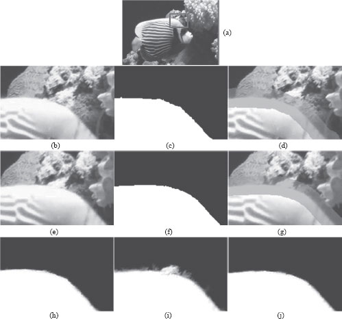
FIGURE 9.9
An example of coherent matting in video. (a) The input sequence, the red box shows the highlighted region in the rest of the figure; (b) the highlighted region on frame t; (c) binary segmentation on frame t; (d) trimap generated on frame t; (e) the highlighted region on frame t + 1; (f) binary segmentation on frame t + 1; (g) trimap generated on frame t + 1; (h) computed α^t, (i) computed α^t+1 without the temporal coherence term in Equation 9.50, (j) computed α^t+1 with the temporal coherence term.

Bibliography

[1]  T. Porter and T. Duff, “Compositing digital images,” in Proc. ACM SIGGRAPH, vol. 18, July 1984, pp. 253–259.

[2]  J. Wang and M. Cohen, “Optimized color sampling for robust matting,” in Proc. IEEE Conf. Computer Vision and Pattern Recognition, 2007, pp. 1–8.

[3]  C. Rother, V. Kolmogorov, and A. Blake, “”grabcut”: Interactive foreground extraction using iterated graph cuts,” ACM Trans. Graphics, vol. 23, no. 3, pp. 309–314, 2004.

[4]  Y. Li, J. Sun, C.-K. Tang, and H.-Y. Shum, “Lazy snapping,” ACM Trans. Graphics, vol. 23, no. 3, pp. 303–308, 2004.

[5]  C. Rhemann, C. Rother, A. Rav-Acha, and T. Sharp, “High resolution matting via interactive trimap segmentation,” in Proc. IEEE Conf. Computer Vision and Pattern Recognition, 2008, pp. 1–8.

[6]  M. Ruzon and C. Tomasi, “Alpha estimation in natural images,” in Proc. IEEE Conf. Computer Vision and Pattern Recognition, 2000, pp. 18–25.

[7]  Y. Mishima, “Soft edge chroma-key generation based upon hexoctahedral color space,” in U.S. Patent 5,355,174, 1993.

[8]  J. Wang and M. Cohen, “Image and video matting: A survey,” Foundations and Trends in Computer Graphics and Vision, vol. 3, no. 2, pp. 97–175, 2007.

[9]  Y.-Y. Chuang, B. Curless, D. H. Salesin, and R. Szeliski, “A Bayesian approach to digital matting,” in Proc. IEEE Conf. Computer Vision and Pattern Recognition, 2001, pp. 264–271.

[10]  A. Levin, D. Lischinski, and Y. Weiss, “A closed-form solution to natural image matting,” IEEE Trans. Pattern Analysis and Machine Intelligence, vol. 30, no. 2, pp. 228–242, 2008.

[11]  L. Grady, T. Schiwietz, S. Aharon, and R. Westermann, “Random walks for interactive alpha-matting,” in Proc. Visualization, Imaging, and Image Processing, 2005, pp. 423–429.

[12]  Y. Guan, W. Chen, X. Liang, Z. Ding, and Q. Peng, “Easy matting: A stroke based approach for continuous image matting,” in Computer Graphics Forum, vol. 25, no. 3, 2006, pp. 567–576.

[13]  J. Wang and M. Cohen, “An iterative optimization approach for unified image segmentation and matting,” in Proc. International Conference on Computer Vision, 2005, pp. 936–943.

[14]  Y. Zheng and C. Kambhamettu, “Learning based digital matting,” in Proc. International Conference on Computer Vision, 2009.

[15]  K. He, C. Rhemann, C. Rother, X. Tang, and J. Sun, “A global sampling method for alpha matting,” in Proc. IEEE Conf. Computer Vision and Pattern Recognition, June 2011, pp. 1–8.

[16]  Y. Boykov, O. Veksler, and R. Zabih, “Fast approximate energy minimization via graph cuts,” IEEE Trans. Pattern Analysis and Machine Intelligence, vol. 23, no. 11, pp. 1222–1239, 2001.

[17]  J. Shi and J. Malik, “Normalized cuts and image segmentation,” IEEE Trans. Pattern Analysis and Machine Intelligence, pp. 888–905, 2000.

[18]  X. He and P. Niyogi, “Locality preserving projections,” in Proc. Advances in Neural Information Processing Systems, 2003.

[19]  D. Singaraju and R. Vidal, “Interactive image matting for multiple layers,” in Proc. IEEE Conf. Computer Vision and Pattern Recognition, 2008, pp. 1–7.

[20]  K. He, J. Sun, and X. Tang, “Single image haze removal using dark channel prior,” in Proc. IEEE Conf. Computer Vision and Pattern Recognition, 2009, pp. 1956–1963.

[21]  E. Hsu, T. Mertens, S. Paris, S. Avidan, and F. Durand, “Light mixture estimation for spatially varying white balance,” ACM Trans. Graphics, vol. 27, pp. 1–7, 2008.

[22]  D. Singaraju, C. Rother, and C. Rhemann, “New appearance models for natural image matting,” in Proc. IEEE Conf. Computer Vision and Pattern Recognition, 2009, pp. 659–666.

[23]  B. Scholkopf and A. J. Smola, Learning with Kernels: Support Vector Machines, Regularization, Optimization, and Beyond. Cambridge, MA, USA: MIT Press, 2001.

[24]  C. Rhemann, C. Rother, and M. Gelautz, “Improving color modeling for alpha matting,” in Proc. British Machine Vision Conference, 2008, pp. 1155–1164.

[25]  X. Bai and G. Sapiro, “Geodesic matting: A framework for fast interactive image and video segmentation and matting,” International Journal on Computer Vision, vol. 82, no. 2, pp. 113–132, 2008.

[26]  E. S. L. Gastal and M. M. Oliveira, “Shared sampling for real-time alpha matting,” Computer Graphics Forum, vol. 29, no. 2, pp. 575–584, May 2010.

[27]  C. Rhemann, C. Rother, J. Wang, M. Gelautz, P. Kohli, and P. Rott, “A perceptually motivated online benchmark for image matting,” in Proc. IEEE Conf. Computer Vision and Pattern Recognition, 2009, pp. 1826–1833.

[28]  C. Barnes, E. Shechtman, A. Finkelstein, and D. B. Goldman, “Patchmatch: A randomized correspondence algorithm for structural image editing,” ACM Trans. Graphics, vol. 28, no. 3, pp. 1–11, July 2009.

[29]  Y. Weiss and W. Freeman, “On the optimality of solutions of the max-product belief propagation algorithm in arebitrary graphs,” IEEE Trans. Information Theory, vol. 47, no. 2, pp. 303–308, 2001.

[30]  S. Kakutani, “Markov processes and the Dirichlet problem,” in Proc. Japanese Academy, vol. 21, 1945, pp. 227–233.

[31]  A. R. Smith and J. F. Blinn, “Blue screen matting,” in Proc. ACM SIGGRAPH, 1996, pp. 259–268.

[32]  P. Villegas and X. Marichal, “Perceptually-weighted evaluation criteria for segmentation masks in video sequences,” IEEE Trans. Image Processing, vol. 13, no. 8, pp. 1092–1103, 2004.

[33]  J. S. Y. Li and H. Shum, “Video object cut and paste,” ACM Trans. Graphics, vol. 24, pp. 595–600, 2005.

[34]  L. Vincent and P. Soille, “Watersheds in digital spaces: an efficient algorithm based on immersion simulations,” IEEE Trans. Pattern Analysis and Machine Intelligence, vol. 13, no. 6, pp. 583–598, 1991.

[35]  D. Titterington, A. Smith, and U. Makov, Statistical Analysis of Finite Mixture Distributions. John Wiley & Sons, 1985.

[36]  A. Blake, C. Rother, M. Brown, P. Perez, and P. Torr, “Interactive image segmentation using an adaptive GMMRF model,” in Proc. European Conference on Computer Vision, 2004, pp. 428–441.

[37]  H. Shum, J. Sun, S. Yamazaki, Y. Li, and C. Tang, “Pop-up light field: An interactive image-based modeling and rendering system,” ACM Trans. Graphics, vol. 23, no. 2, pp. 143–162, 2004.

[38]  J. Wang, P. Bhat, R. A. Colburn, M. Agrawala, and M. F. Cohen, “Interactive video cutout,” ACM Trans. Graphics, vol. 24, pp. 585–594, 2005.

[39]  D. Comaniciu and P. Meer, “Mean shift: A robust approach toward feature space analysis,” IEEE Trans. Pattern Analysis and Machine Intelligence, vol. 24, no. 5, pp. 603–619, 2002.

[40]  Y.-Y. Chuang, A. Agarwala, B. Curless, D. Salesin, and R. Szeliski, “Video matting of complex scenes,” ACM Trans. Graphics, vol. 21, pp. 243–248, 2002.

[41]  R. Szeliski and H. Shum, “Creating full view panoramic mosaics and environment maps,” in Proc. ACM SIGGRAPH, 1997, pp. 251–258.

[42]  X. Bai, J. Wang, D. Simons, and G. Sapiro, “Video snapcut: Robust video object cutout using localized classifiers,” ACM Trans. Graphics, vol. 28, no. 3, pp. 1–11, July 2009.

¹In many applications, recovering α_p alone is sufficient. We will mainly focus on how to recover the alpha matte in this chapter.

²For notation simplicity, we will use υ_i to denote both an unknown pixel and its corresponding node in the graph.