11

Hierarchical Graph Encodings

Luc Brun

GREYC UMR CNRS 6072

ENSICAEN

Caen, France

Email: [email protected]

Walter Kropatsch

Pattern Recognition and Image Processing Group

Vienna University of Technology

Vienna, Austria

Email: [email protected]

CONTENTS

11.1  Introduction

11.2  Regular Pyramids

11.3  Irregular Pyramids Parallel construction schemes

11.3.1  Maximal Independent Set

11.3.2  Maximal Independent Vertex Set

11.3.2.1  Definition of Reduction Window

11.3.3  Data-Driven Decimation Process

11.3.4  Maximal Independent Edge Set

11.3.5  Maximal Independent Directed Edge Set

11.3.6  Comparison of MIVS, MIES, and MIDES

11.4  Irregular Pyramids and Image properties

11.4.1  Relating Regions

11.4.2  Graph models

11.4.2.1  Simple Graph

11.4.2.2  Dual Graph Model

11.4.2.3  Combinatorial Maps

11.4.3  Simple Graph Pyramids

11.4.4  Dual Graph Pyramids

11.4.4.1  Contraction Kernel

11.4.4.2  Dual Graph pyramids and Topological relationships

11.4.5  Combinatorial Pyramids

11.4.5.1  Relationships between regions

11.4.5.2  Implicit Encoding of a Combinatorial Pyramid

11.4.5.3  Dart’s Embedding and Segments

11.5  Conclusion

Bibliography

11.1  Introduction

Regular image pyramids have been introduced in 1981/82 [1] as a stack of images with decreasing resolutions. Such pyramids present interesting properties for image processing and analysis such as [2] the reduction of noise, the processing of local and global features within the same frame, the use of local processes to detect global features at low resolution, and the efficiency of many computations on this structure. Regular pyramids are usually made of a very limited set of levels (typically log(n) where n is the diameter of the input image). Therefore, if each level is constructed in parallel from the level below, the whole pyramid may be built in O(log(n))$\mathcal{O}\left(\log \left(n\right)\right)$ parallel steps. The systematic construction establishes a strong relation between the levels enabling a quick top-down access to every pixel of the original image. However, the regular structure of such pyramids induce several drawbacks such as the limited number of regions which may be encoded at a given level or the fact that a small shift of an initial image may induce important modifications of its associated regular pyramid.

Irregular pyramids overcome these negative properties while keeping the main advantages of their regular ancestors. Such pyramids are defined as a stack of successively reduced graphs. Each vertex of such a pyramid being defined from a connected set of vertices in the graph below. Typically, such graphs encode the pixel’s neighborhood, the region adjacency, or a particular semantic of image objects. Since 2D images correspond to a sampling of the plane, such graphs are embeded in the plane by definition.

The construction of such pyramids raises two questions: (1) How to build efficiently each level of the pyramid from the one below? (2) Which properties of the plane are captured at each level? This chapter provides answers to both questions together with an overview of hierarchical models. We first present in Section 11.2 the regular pyramid framework. We then present the main parallel construction schemes of irregular pyramids in Section 11.3. These construction schemes determine an important “vertical” property of an irregular pyramid: the speed at which the size of graphs decreases between the different levels of the pyramid. The main graph encodings used within the irregular pyramid framework together with image properties captured by such models are presented in Section 11.4. Image properties captured by a given graph model may be considered as horizontal’s properties of a pyramid. Each combination of a parallel construction scheme (Section 11.3) with a graph encoding (Section 11.4) defines an irregular pyramid model with specific vertical and horizontal properties.

11.2  Regular Pyramids

A regular pyramid is defined as a sequence of images with an exponentially decreasing resolution. Each image of such a sequence is called a level of the pyramid. The first level, called the base of the pyramid, corresponds to the original image, while the top of the pyramid corresponds usually to a single pixel whose value is a weighted mean of pixels belonging to the base. Using image neighborhood relationships, a reduction window connects any pixel of the pyramid to a set of pixels defined at the level below. Any pixel of a pyramid is considered as the parent of the pixels belonging to its reduction window (filled circles in Figure 11.1). Conversely, all pixels within a reduction window are considered as the children of the pixel associated to this reduction window in the above level. The parent/child or hierarchical relationship may be extended between any two level using the transitive closure of the relationship induced by the reduction window. The set of pixels in the base level image associated to a given pixel of the pyramid is called its receptive field. Let us, for example, consider the top-left pixel in Figure 11.1(c). Its reduction window and receptive field are the top left 2 × 2 and 4 × 4 windows of the image in Figure 11.1(b) and (a) respectively.

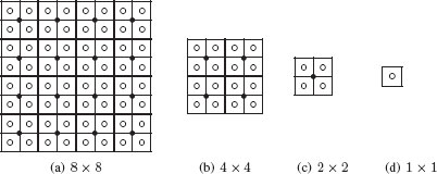
FIGURE 11.1
A 2 × 2/4 regular pyramid.

One additional important parameter of a regular pyramid is the decimation ratio (also called reduction factor) which encodes the ratio between the size of two successive images. This ratio remains the same between any two successive levels of the pyramid. A reduction function determines the value of any pixel of the pyramid from the value of its children defining its reduction window (Figure 11.2). A regular pyramid may thus be formally defined as the ratio N × N/q, where N × N represent the size of the reduction window, while q represents the decimation ratio. Different types of pyramid may be distinguished according to the value of N × N/q:

•  If N × N/q < 1, the pyramid is named a nonoverlapping holed pyramid. Within such a pyramid, some pixels have no parent [3] (e.g., the center pixel in Figure 11.3(a));

•  If N × N/q = 1, the pyramid is called a nonoverlapping pyramid without hole (see, e.g., in Figure 11.3(b)). Within such pyramids, each pixel in the reduction window has exactly one parent [3];

•  If N × N/q > 1, the pyramid is named an overlapping pyramid (see, e.g., in Figure 11.3(c)). Each pixel of such a pyramid has on average N²/q parents [1]. If each child selects one parent, the set of children in the reduction window of each parent is rearranged. Consequently, the receptive field may take any form inside the original receptive field.

Regular pyramids have several interesting properties enumerated by Bister [2]:

1.  Reduction functions are usually defined as low-pass filters, hence inducing a robustness against noise in high levels of the pyramid;

2.  Algorithms insensitive to image resolution may be readily designed using the pyramid framework;

3.  Global properties in the base level image become local at higher levels in the hierarchy and may thus be detected using local filters;

4.  Top-down analysis of the content of a pyramid may be achieved efficiently using a divide and conquer strategy;

5.  Objects to be detected may be retrieved using low resolution images with a simplified image content.

Despite these interesting properties, regular pyramids have several limitations. Indeed, the bounded size and fixed shape of the reduction window induce rigid constraints on the data structure which may not allow it to readily handle the variability of image content. Regular pyramids are, for example, quite sensitive to small image shifts due to the fixed locations of reduction window (this is called the shift dependence problem). Moreover, the fixed size of reduction windows bounds artificially the number of regions that may be encoded at a given level and does not allow us to readily encode elongated objects.

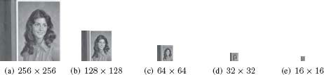
FIGURE 11.2
A 2 × 2/4 pyramid whose reduction function is defined as a Gaussian centered on the center of the reduction window. The size of each image is indicated below.

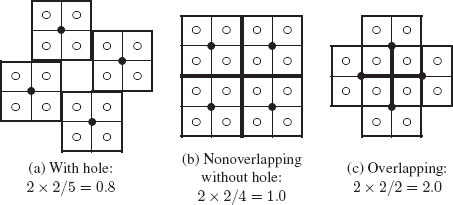
FIGURE 11.3
Three different types of regular pyramids.

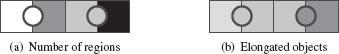
FIGURE 11.4
Two 1 × 4/2 image pyramids based on a 1 × 4 base level image. These two figures illustrate the limited number of objects which may be defined at a given level of a pyramid (a) and the difficulties encountered by such pyramids to encode elongated objects(b).

This last drawback is illustrated in Figure 11.4(a). The base of the pyramid is a 1 × 4 image encoding a single line composed of 4 pixels with different colors. These pixels correspond to different regions that should be keep by a segmentation process. However, using an image pyramid with a reduction factor equal to 2, only 2 pixels can survive at level 1. Two regions defined at the base level should thus be removed at level one, this result being independent of the gray level differences between pixels. Figure 11.4(b) illustrates the difficulty encountered by regular pyramids to encode elongated objects. The 1 × 4 base level image is composed of pixels with close values which should be grouped into a single entity by a segmentation process. Using a 1 × 4/2 image pyramid, these 4 pixels are merged into two pixels at level 1. This merging operation artificially increases the gray level difference between pixels, hence producing two distinct regions at level 1.

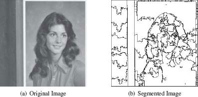
FIGURE 11.5
Image segmentation of Girl test image using the pyramid linking algorithm [2] with an overlapping 5 × 5/4 pyramid.

This phenomenon is also illustrated in Figure 11.5 on a real image using Bister algorithm [2] on a 5 × 5/4 pyramid. As shown in Figure 11.4(b), several elongated regions located on the top and the left part of the image together with the hair of girl are artificially split into several small regions.

Let us finally temper the above remarks by noting that Bister [2] always managed to adapt the regular pyramid to the class of images to process. However, such an adaptation of the reduction window, decimation ratio, reduction function… should be performed for each image class on an heuristic basis. We can additionally note that some drawbacks of regular pyramids may become advantages on some specific applications. For example, the fact that regular pyramids do not readily allow us to encode elongated objects may become an advantage in fields where objects to be detected are known to be compact. Such an example of application is provided by Rosenfeld [4] who uses a regular pyramid in order to detect vehicles in infrared images. Within this particular context, vehicles are known to be compact and may be detected as single pixels at some levels of the pyramid.

11.3  Irregular Pyramids Parallel construction schemes

Irregular pyramids have been first proposed by Meer and Montanvert et al. [5] in order to overcome negative properties of their regular ancestors while keeping their main advantages. More particularly, two important advantages of regular pyramids over nonhierarchical image processing algorithms should be preserved:

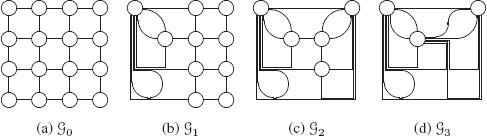
FIGURE 11.6
First levels of an irregular pyramid using the 4-adjacency of pixels.

•  Property I. The bottom-up computation of any pyramid may be performed in parallel, each pixel computing its value from its child independently;

•  Property II. Due to the fixed size of the decimation ratio, the height of a pyramid is equal to a log of the image size. Therefore, using a parallel computation scheme any pyramid may be computed in $\mathcal{O}\left(\log \left(\left|I\right|\right)\right)$ parallel steps, where |I| denotes the size of the base level image.

On the other hand, the main drawbacks of regular pyramids are the fixed shape of reduction windows and the fixed neighborhood of each pixel which do not allow us to readily adapt the pyramid to the data and to preserve adjacency relationships along the pyramid. In order to overcome these drawbacks, Meer and Montanvert et al. [5] defined irregular pyramids as stacks of successively reduced graphs (${\mathcal{G}}_0,{\mathcal{G}}_1,{\mathcal{G}}_2,{\mathcal{G}}_3$ in Figure 11.6). Such pyramids may adapt the shape of the reduction window to the data and preserve adjacency relationships between regions through graph encoding since a vertex may have an arbitrary number of neighbors. In reference to their regular ancestors, the decimation ratio of irregular pyramids is usually defined as the mean value of the ratio between the number of vertices of two successive graphs $\left(\frac{\left|{\mathcal{V}}_l\right|}{\left|{\mathcal{V}}_{l+1}\right|}\right)$ when this last term is approximately constant along the pyramid. The construction of a graph ${\mathcal{G}}_{l+1}=\left({\mathcal{V}}_{l+1},{ℰ}_{l+1}\right)$ from ${\mathcal{G}}_l=\left({\mathcal{V}}_l,{ℰ}_l\right)$, is performed through the following steps:

•  Step I. Define a partition of ${\mathcal{V}}_l$ into a set of connected components. A vertex of ${\mathcal{G}}_{l+1}$ is created and attached to each connected component of this partition. The connected component attached to each vertex of ${\mathcal{G}}_{l+1}$ is called its reduction window in reference to regular pyramids;

•  Step II. Define adjacency relationships between vertices of ${\mathcal{G}}_{l+1}$ from adjacency relationships between the connected components of ${\mathcal{V}}_l$’s partition.

This section is devoted to parallel reduction schemes which are uniquely concerned by the first step of the above construction scheme, the second step being detailed in Section 11.4. Sequential reduction schemes such as [6] violate Property I (Section 11.3) and are thus not considered in this chapter. This section describes global reduction schemes of a graph. Such global reduction schemes may, however, be easily restricted according to some segmentation criterion (e.g., [7]) by removing from the initial set of edges ${ℰ}_0$ all edges encoding adjacency relationships between vertices which should not merge according to a segmentation criterion.

Note that the number of connected components defining a partition of ${\mathcal{G}}_l$ defines the cardinality of ${\mathcal{V}}_{l+1}$ and hence the decimation ratio (also called reduction factor) of irregular pyramids. Several parallel methods have been proposed to ensure a constant value to the decimation ratio $\left(\frac{\left|{\mathcal{V}}_l\right|}{\left|{\mathcal{V}}_{l+1}\right|}\right)$, all these methods being based on the notion of maximal independent set.

11.3.1  Maximal Independent Set

Let us consider a finite or enumerable set $\mathcal{X}$ provided with a symmetric neighborhood function $\mathcal{N}:\mathcal{X}\to \mathcal{P}\left(X\right)$, where $\mathcal{P}\left(\mathcal{X}\right)$ denotes the powerset of $\mathcal{X}$. An independent set of $\mathcal{X}$ is a subset $\mathcal{J}$ of $\mathcal{X}$ such that no elements of $\mathcal{J}$ are related by the neighborhood function $\mathcal{N}(.)$:

$\forall \left(x,y\right)\in {\mathcal{J}}^2,x\notin \mathcal{N}\left(y\right)$

(11.1)

An independent set is said to be maximal if it is not the subset of any independent set. For example, the set of even numbers, is a maximal independent set over the set of natural integers provided with the neighborhood relationship : $\mathcal{N}\left(n\right)=\left\{n-1,n+1\right\}$. Note that, both even and odd integers define a maximal independent set using this neighborhood relationship. A maximal independent set is thus not unique. Moreover, given a maximal independent set $\mathcal{J}$, any element x in $X-\mathcal{J}$ must be adjacent to some element of $\mathcal{J}$, otherwise x could be added to $\mathcal{J}$ hence violating the maximal property. Conversely, if $\mathcal{J}$ is a nonmaximal independent set, at least one element x may be added to $\mathcal{J}$. This element is not adjacent to any element of $\mathcal{J}$ due to condition 11.1. The maximality of an independent set may thus be characterized by:

$\forall x\in X-\mathcal{J},\exists y\in \mathcal{J}|x\in \mathcal{N}\left(y\right)$

(11.2)

Within the irregular pyramid framework elements of a maximal independent set are usually called surviving elements. Condition 11.1, states that two adjacent elements cannot both survive. On the other hand, condition 11.2 states that any nonsurviving element should be adjacent to a surviving one. A maximal independent set may thus be interpreted as a subsampling of the initial set $\mathcal{X}$ according to the neighborhood relationship $\mathcal{N}$. Let us, for example, consider the case where $\mathcal{X}$ corresponds to the set of pixels of an image, while the neighborhood relationship encodes the 8 connectivity of pixels. A maximal independent set may then be achieved by selecting one pixel every two lines and two columns. One may easily check in Figure 11.7 that surviving pixels (■) are not adjacent (condition 11.1) and that any nonsurviving pixel (□) is adjacent to at least one surviving pixel (condition 11.2).

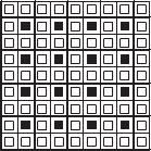
FIGURE 11.7
A maximal independent set (■) over a planar sampling grid with the 8 neighborhood.

The remainder of this chapter will be devoted to finite sets. Given such a finite set $\mathcal{X}$, an independent set will be called maximum if its cardinal is maximum over all possible maximal independent sets. Moreover, in such a case, neighborhood relationships may be encoded by a graph $\mathcal{G}=\left(\mathcal{X},ℰ\right)$, where $\left(u,\upsilon \right)\in {\mathcal{X}}^2$ belongs to $\mathcal{E}$ if and only if $u\in \mathcal{N}\left(\upsilon \right)$.

11.3.2  Maximal Independent Vertex Set

A maximal independent vertex set (MIVS) of a graph ${\mathcal{G}}_l=\left({\mathcal{V}}_l,{ℰ}_l\right)$ is defined as a maximal independent set over the set ${\mathcal{V}}_l$ using the neighborhood relationship induced by ${ℰ}_l$. If we denote the maximal independent set by ${\mathcal{V}}_{l+1}$, conditions 11.1 and 11.2 may be written as follows:

$\forall \left(\upsilon ,{\upsilon }^{\prime }\right)\in {ℰ}_l:\left(\upsilon ,{\upsilon }^{\prime }\right)\notin {ℰ}_l$

(11.3)

$\forall \upsilon \in {\mathcal{V}}_l-{\mathcal{V}}_{l+1}\exists {\upsilon }^{\prime }\in {\mathcal{V}}_{l+1}:\left(\upsilon ,{\upsilon }^{\prime }\right)\in {ℰ}_l$

(11.4)

The construction scheme of such a maximal independent set was introduced by Meer [8] as an iterative stochastic process based on the outcome of a random variable attached to each vertex and uniformly distributed over [0, 1]. Any vertex corresponding to a local maximum of the random variable is then considered as a surviving vertex. One iteration of this process allows us to satisfy condition (11.3) and hence to obtain an independent set, since two adjacent vertices cannot both correspond to local maxima. However, one vertex not corresponding to a local maximum may have no surviving vertices in its neighborhood. In other terms, such a process may lead to a nonmaximal independent set. Such a configuration is illustrated on Figure 11.8 where values inside each vertex represent the outcome of the random variable. Vertices with value 9 represent local maxima of the random variable and are thus selected as survivors. Vertices 7 and 8 adjacent to a surviving vertex cannot be selected as survivors due to condition (11.3). Vertex 6 does not correspond to a maximum of the random variable. This vertex must nevertheless be selected as a survivor in order to fulfill condition (11.4) and obtain a maximal independent set.

We should thus iterate the selection of local maxima until both conditions (11.3) and (11.4) are satisfied. Such an iterative process requires us to attach three variables x_i, p_i, q_i to each vertex ${\upsilon }_i\in {\mathcal{V}}_l$. Variable x_i encodes the outcome of the random variable attached to υ_i, while p_i and q_i correspond to Boolean variables whose values encode the following states:

FIGURE 11.8
Construction of a maximal independent vertex set on a 1D graph. Surviving vertices are shown by double circles.

•  If p_i is true, υ_i is considered as a surviving vertex;

•  If q_i is true, υ_i is a candidate which may become a surviving vertex at some further iteration. Conversely, if q_i is false, υ_i is considered as a nonsurviving vertex.

Let ${\left(p_i^{\left(k\right)}\right)}_{k\in \left\{1,\dots ,n\right\}}$ and ${\left(q_i^{\left(k\right)}\right)}_{k\in \left\{1,\dots ,n\right\}}$ denote values taken by variables p_i and q_i along the iteration of our iterative algorithm. Variable p_i and q_i are initialized as follow

$\begin{array}{ll}{p}_i^{\left(1\right)}\hfill & =x_i={\max }_{{\upsilon }_j\in \mathcal{N}\left({\upsilon }_i\right)}\left\{x_j\right\}\hfill \\ q_i^{\left(1\right)}\hfill & ={{\displaystyle \bigwedge }}_{{\upsilon }_j\in \mathcal{N}\left({\upsilon }_i\right)}{\overline{p_j}}^{\left(1\right)}\hfill \end{array}$

(11.5)

where $\mathcal{N}\left({\upsilon }_i\right)$ denotes the neighborhood of υ_i and $\bigwedge$ corresponds to the logical “and” operator. We suppose by convention that ${\upsilon }_i\in \mathcal{N}\left({\upsilon }_i\right)$.

Equation (11.5) states that a vertex survives $\left(p_i^{\left(1\right)}=\text{true}\right)$ if it corresponds to a maxima of the random variable. One vertex is a candidate $\left(q_i^{\left(1\right)}=\text{true}\right)$ if it is not already a survivor and if none of its neighbors survive.

The iterative update of the predicate p_i and q_i is performed using the following rules:

$\begin{array}{ll}{p}_i^{\left(k+1\right)}\hfill & =p_i^{\left(k\right)}\vee \left(q_i^{\left(k\right)}\wedge x_i=\max \left\{x_j|{\upsilon }_j\in \mathcal{N}\left({\upsilon }_i\right)\wedge q_j^{\left(k\right)}\right\}\right)\hfill \\ q_i^{\left(k+1\right)}\hfill & ={{\displaystyle \bigwedge }}_{{\upsilon }_j\in \mathcal{N}\left({\upsilon }_i\right)}{\overline{p_j}}^{\left(k+1\right)}\hfill \end{array}$

(11.6)

where ∨ denotes the logical “or” operator.

One vertex surviving at iteration k thus remain a survivor at further iterations $\left(p_i^{\left(k+1\right)}=p_i^{\left(k\right)}\vee \dots \right)$. Moreover, a candidate $\left(q_i^{\left(k\right)}=\text{true}\right)$ may become a survivor if it corresponds to a local maxima of all the candidates in its neighborhood $\left(x_i=\max \left\{x_j|{\upsilon }_j\in \mathcal{N}\left({\upsilon }_i\right)\wedge q_j^{\left(k\right)}\right\}\right)$. Finally, a candidate remains in this state $\left(q_i^{\left(k+1\right)}=\text{true}\right)$ if it does not become a survivor and if none of its neighbors are selected as a survivor.

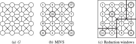
FIGURE 11.9
Construction of a maximal independent vertex set using a random variable on a graph $\mathcal{G}$ encoding a 4 × 4 8-connected sampling grid (a). The outcome of the random variable is displayed inside each vertex. Surviving vertices are surrounded by nested circles (b). Reduction windows associated to surviving vertices (c).

Note that the set of vertices such that $p_i^{\left(k\right)}=\text{true}$ defines an independent set at any step k of this iterative algorithm. Each step decreases the number of candidates and increases the number of survivors until no more survivors may be added. The set of survivors then define a maximal independent set. Let us additionally note that this process is purely local. Indeed, for each iteration, each vertex updates the values of p_i and q_i according to the one of its neighbors. Such a process may thus be easily encoded on a parallel machine. Figure 11.9 (b) shows the outcomes of the random variable on a graph defined from the 4 × 4 8-connected sampling grid (Figure 11.9 (a)). Surviving vertices are surrounded by an extra circle.

Jolion [9] improves the adaptability of the above decimation process by defining surviving vertices as local maxima of an interest operator. For example, within the segmentation framework, Jolion defines the operator of interest as a decreasing function of the gray level variance computed in the neighborhood of each vertex. This operator provides a location of surviving vertices in homogeneous regions.

11.3.2.1  Definition of Reduction Window

Given the set of surviving vertices, constraint (11.3) of a MIVS insures that each nonsurviving vertex is adjacent to at least one survivor. The selection of a surviving parent by each nonsurviving vertex may be performed using various heuristics. Meer [8] and Montanvert et al. [5] connect each nonsurviving vertex to its surviving neighbor with the greatest value of the random variable. Jolion [9] uses a contrast measure such as the gray level difference, to link each nonsurviving vertex to its least contrasted surviving neighbor. Each surviving vertex is thus the parent of all nonsurviving vertices attached to it. Figure 11.9(c) shows the reduction window defined from Figure 11.9(b) by connecting each nonsurviving vertex to its surviving neighbor of greatest value.

Given the partition of ${\mathcal{V}}_l$ into a set of reduction window with their associated survivors ${\mathcal{V}}_{l+1}$, the reduced graph ${\mathcal{G}}_{l+1}=\left({\mathcal{V}}_{l+1},{ℰ}_{l+1}\right)$ is defined using heuristics defined in Section 11.4.

11.3.3  Data-Driven Decimation Process

As mentioned in Section 11.3.2, a vertex selected as a survivor remains in this state until the end of the iterative construction scheme of a MIVS (equation 11.6). Moreover, the neighbors of such a survivor are classified as noncandidates and remain also in this state until the end of the iterative process. Therefore, one surviving vertex together with its nonsurviving neighbors could be reduced into a single vertex of the reduced graph as soon as it is classified as a survivor at some iteration step. However, using the construction scheme defined in Section 11.3.2, the definition of a reduced graph using a MIVS and requires that all the vertices of a graph are marked as survivors or noncandidate. For important graphs, this latency which is proportional to the number of iterations may be important.

The data-driven decimation process (D3P) proposed by Jolion [10] is based on a single iteration of the iterative decimation process (Equation 11.6) at each level of the pyramid. The two variables p_i and q_i defined in Section 11.3.2 keep the same meaning but are now global to the whole pyramid. These variables are initialized to true at the base level of the pyramid:

$p_i^1=q_i^1=\text{true},\forall {\upsilon }_i\in {\mathcal{V}}_0$

(11.7)

where ${\mathcal{G}}_0=\left({\mathcal{V}}_0,{ℰ}_0\right)$ encodes the base of the pyramid.

The update of variables p_i and q_i between each level is performed using the following equations:

$\begin{array}{ll}{p}_i^{\left(k+1\right)}\hfill & =\left(\left(p_i^{\left(k\right)}\vee q_i^{\left(k\right)}\right)\wedge x_i=\max \left\{x_j|q_j^{\left(k\right)}\wedge {\upsilon }_j\in {\mathcal{N}}_k\left({\upsilon }_i\right)\right\}\right)\hfill \\ q_i^{\left(k+1\right)}\hfill & ={{\displaystyle \bigwedge }}_{{\upsilon }_j\in {\mathcal{N}}_k\left({\upsilon }_i\right)}{\overline{p_j}}^{k+1}\wedge {\mathcal{N}}_k\left({\upsilon }_i\right)\ne \left\{{\upsilon }_i\right\}).\hfill \end{array}$

(11.8)

In other terms, a vertex υ_i is selected as a survivor $\left(p_i^{\left(k+1\right)}=\text{true}\right)$, if it was a survivor or a candidate in graph ${\mathcal{G}}_k\left(p_i^{\left(k\right)}\vee q_i^{\left(k\right)}\right)$ and if it corresponds to a maximum of the random variable among the candidates in ${\mathcal{N}}_k\left({\upsilon }_i\right)\left(x_i=\max \left\{x_j|q_j^{\left(k\right)}\wedge {\upsilon }_j\in {\mathcal{N}}_k\left({\upsilon }_i\right)\right\}\right)$. A vertex of ${\mathcal{G}}_k$ becomes a candidate if it is not adjacent to any surviving vertex and if it is not isolated $\left({\mathcal{N}}_k\left({\upsilon }_i\right)\ne \left\{{\upsilon }_i\right\}\right)$.

The set of surviving vertices determined by Equation (11.8) defines an independent set over ${\mathcal{G}}_k$. This set is, however, usually nonmaximal. More precisely, we may decompose the set ${\mathcal{V}}_k$ into three subsets based on variables $p_i^{\left(k+1\right)}$ and $q_i^{\left(k+1\right)}$: Survivors $\left(p_i^{\left(k+1\right)}=\text{true}\right)$, candidates $\left(q_i^{\left(k+1\right)}=\text{true}\right)$, and noncandidates $\left(q_i^{\left(k+1\right)}=\text{false}\right)$. Noncandidate vertices are adjacent to at least one survivor (Equation 11.8). These vertices together with surviving vertices are grouped into reduction windows reduced into a single vertex in graph ${\mathcal{G}}_{k+1}$. Candidate vertices represent the set of vertices which would have been classified as survivors or nonsurvivors at further iteration steps using the iterative construction scheme of a MIVS (equation 11.6). Using the D3P construction scheme, the classification of such vertices is delayed to higher levels of the pyramid. The set of vertices defined at level k + 1 is thus equal to the set of survivors together with the set of candidates:

${\mathcal{V}}_{k+1}=\left\{{\upsilon }_i\in {\mathcal{V}}_k|p_i^{\left(k+1\right)}\vee q_i^{\left(k+1\right)}\right\}.$

(11.9)

The set ${ℰ}_{k+1}$ is defined according to various heuristics defined in Sections 11.4.3 and 11.4.4. Equation (11.8) is then applied on the reduced graph ${\mathcal{G}}_{k+1}=\left({\mathcal{V}}_{k+1},{ℰ}_{k+1}\right)$ until the top of the pyramid.

Let us recall (Section 11.3.2) that Jolion [9] defines surviving vertices as local maxima of an interest operator. One main advantage of the D3P is that vertices corresponding to strong local maxima of the interest operator are detected and merged with their nonsurviving neighbors at low levels of the pyramid. Remaining candidates which correspond to more complex configurations are detected at higher levels of the pyramid where the content of the graph is already simplified hence simplifying the decision process. For example, within a segmentation scheme, the interest operator may detect the center of homogeneous regions which grow at low levels of the pyramid in order to facilitate the aggregation of vertices encoding pixels on the boundary of two regions. Let us additionally note that this asynchronous decimation process is consistent with some psychovisual experiments [11] showing that our brain uses asynchronous processes.

11.3.4  Maximal Independent Edge Set

Within the MIVS framework (Section 11.3.2), two surviving vertices cannot be adjacent. The number of surviving vertices defining a MIVS is thus highly dependent of the connectedness of the graph. Moreover, using the stochastic construction scheme of a MIVS defined by Meer [8] and Montanvert et al. [5] one vertex is defined as a survivor if it corresponds to a local maxima of a random variable. The probability that a vertex survives is thus relative to the size of its neighborhood. Adjacency relationships have thus an influence on:

1.  The height of the pyramid

2.  The number of iterations required to build each level of the pyramid from the previous one

Several experiments performed by Kropatsch et al. [12, 13] have shown that the mean degree of vertices increases along the pyramid. This increasing connectivity induces the selection of a decreasing number of surviving vertices and hence decreases the decimation ratio along the pyramid.

Such a decrease of the decimation ratio increases the height of the pyramid and thus violates one of the two main properties of regular pyramids that irregular pyramids should preserve (Section 11.3): The logarithmic height of the pyramid according to the size of its base.

In order to correct this important drawback, Kropatsch et al. [12, 13] propose to base the decimation of a pyramid on the construction of a forest $ℱ$ of $\mathcal{G}$ such that:

•  Cond. I. Any vertex of $\mathcal{G}$ belongs to exactly one tree of $\mathcal{F}$

•  Cond. II. Each tree is composed of at least two vertices.

Each tree of $\mathcal{F}$ defines a reduction window on which a surviving vertex is selected. Remaining vertices of the tree are considered as nonsurviving vertices. (Cond. I.) insures that each vertex is classified either as a survivor or as a nonsurvivor. (Cond. II.) insures that the number of vertices decreases by a factor at least 2, hence providing a reduction factor at least equal to 2.

The first step toward the construction of the forest $\mathcal{F}$ is based on the notion of maximal independent edge set (MIES). Given a graph $\mathcal{G}=\left(\mathcal{V},ℰ\right)$, a maximal independent edge set corresponds to a maximal independent vertex set on the edge graph $\mathcal{G}=\left(ℰ,{ℰ}^{\prime }\right)$ where ${ℰ}^{\prime }$ is defined using the following neighborhood relationship on $\mathcal{E}$:

$\forall \left(e_{u\upsilon },e_{xy}\right)\in {ℰ}^2{e}_{u\upsilon }\in \mathcal{N}\left(e_{xy}\right)\text{iff}\left\{u,\upsilon \right\}\cap \left\{x,y\right\}\ne \cancel{0}$

(11.10)

where e_u,υ denotes an edge between vertices u and υ.

Using equation 11.10, two edges are said to be neighbors if they are incident to a same vertex. The set of surviving edges defined by this decimation process corresponds to a maximal matching of the initial graph $\mathcal{G}=\left(\mathcal{V},ℰ\right)$ (Definition 1 and Figure 11.10).

Definition 1

Given a graph $G=\left(\mathcal{V},ℰ\right)$, a subset of edges $\mathcal{C}\subset ℰ$ is a matching if none of the edges of $\mathcal{C}$ are incident to a same vertex. Let us call the necessary property of $\mathcal{C}$ the matching property.

Maximal matching: A matching is said to be maximal if no edge may be added to the set without violating the matching property;

Maximum matching: A maximum matching is a matching that contains the largest possible number of edges;

Perfect matching: A matching $\mathcal{C}$ is perfect if any vertex is incident to an edge of $\mathcal{C}$. Any perfect matching is maximum.

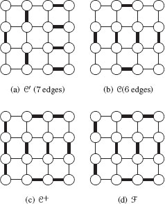
FIGURE 11.10
Two maximal matchings with different numbers of edges (a), (b). Surviving edges are drawn by thick lines. The augmented set ${\mathcal{C}}^{+}$ (c) and the final forest $\mathcal{F}$ (d).

A vertex incident to an edge of a matching is said to be saturated. Otherwise, it is unsaturated.

Note that a maximal matching $\mathcal{C}$ does not contain any loop and thus corresponds to a forest of the graph $\mathcal{G}$. However, $\mathcal{C}$ is usually not perfect (Definition 1) and thus violates (Cond. I., Section 11.3.4) since unsaturated vertices do not belong to any tree of our forest. Let us consider such an unsaturated vertex υ and a non-self-loop edge e_υ,w incident to υ. The matching $\mathcal{C}$ being maximal, w must be incident to one edge of $\mathcal{C}$. The set $C\cup \left\{e_{\upsilon ,w}\right\}$ is still a forest of $\mathcal{G}$ and contains the previously unsaturated vertex υ. Let us consider the ${\mathcal{C}}^{+}$, obtained from $\mathcal{C}$ by adding edges connecting unsaturated vertices to $\mathcal{C}$. The set ${\mathcal{C}}^{+}$ is no more a matching. However, by construction, ${\mathcal{C}}^{+}$ is a spanning forest of $\mathcal{G}$ composed of trees of depth 1 or 2. Trees of depth 2 may be decomposed in two trees of depth 1 by removing from ${\mathcal{C}}^{+}$ edges both end-points of which are incident to some other edges of ${\mathcal{C}}^{+}$.

The resulting set $\mathcal{F}$ is a spanning forest of $\mathcal{G}$ composed of trees of depth 1. One vertex may thus be selected in each tree such that the tree rooted on this vertex has a depth 1. Selected vertices correspond to surviving vertices, while remaining vertices are classified as nonsurvivors.

The main motivation of this method is to provide a better stability of the reduction factor. The problem identified within the MIVS framework being connected to the vertex degree, the proposed method uses the notion of maximal independent edge set to avoid the use of vertex’s neighborhood. Experiments provided by Haxhimusa et al. [12] (Section 11.3.6) show that the decimation ratio remains close to 2 along the pyramid.

11.3.5  Maximal Independent Directed Edge Set

Using the maximal independent edge set framework (Section 11.3.4), surviving vertices are selected so as to obtain rooted trees of depth one. Such a selection scheme is thus induced by the decomposition of the initial graph into trees and cannot readily incorporate a priori constraints concerning surviving vertices. However, in some applications, the definition of the surviving vertex within each reduction window is an important issue. For example, within the analysis of line drawing framework [14], end points of a line or intersection points must be preserved, and hence selected as survivors, for geometric accuracy reasons.

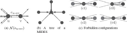
FIGURE 11.11
Directed neighborhood $\mathcal{N}\left(e_{u\to \upsilon }\right)$ of edge e_u→υ(a). A tree of a MIDES defining unambiguously its surviving vertex (b). Two edges within a same neighborhood cannot be both selected. Hence, red edges in (c) cannot be selected once black edges have been added to the MIDES.

In order to provide a better selection of surviving vertices, Kropatsch et al [12], propose to adapt the MIES framework as follows: The decimation of a graph is based on the construction of a spanning forest $ℱ$ such that:

•  Cond. I. Any vertex of the graph belongs to exactly one tree of $ℱ$ of depth one

•  Cond. II. Each tree is encoded using directed edges. Its surviving vertex is defined either as the only vertex of the tree or as the unique target of all tree’s edges (Figure 11.11(b)).

Each tree of $ℱ$ defining a reduction window, (Cond. I., Section 11.3.5) insures that the set of reduction windows encodes a partition of the vertex set of the graph. Moreover, the surviving vertex within each tree is uniquely determined by (Cond. II., Section 11.3.5). Such a use of directed edges provides a simple way to constraint the selection of surviving vertices by restricting the construction of the forest $ℱ$ to edges encoding possible selection of surviving and nonsurviving vertices. Such edges are called preselected edges.

Note that any undirected graph may be converted into a directed graph by transforming each of its undirected edges e_u,υ into a pair of directed reverse edges e_u→υ and e_υ→u with opposite sources and targets. However, the set of preselected edges of such a graph may contain e_u→υ without containing e_υ→u. Let us denote by $\mathcal{G}=\left(\mathcal{V},ℰ\right)$ the directed subgraph induced by the set of preselected edges $ℰ$. The first step toward the construction of the spanning forest $ℱ$ consists to build a maximal independent set on $ℰ$ using the following directed edge’s neighborhood relationship (Figure 11.11(a)):

Definition 2

Let e_u→υ be a directed edge of $\mathcal{G}$ with u ≠ υ. The directed neighborhood $\mathcal{N}\left(e_{u\to \upsilon }\right)$ is given by all directed edges with the same source u, targeting the source u or emanating from the target υ:

$\mathcal{N}\left(e_{u\to \upsilon }\right)=\left\{e_{u\to w}\in E\right\}\cup \left\{e_{w\to u}\in E\right\}\cup \left\{e_{\upsilon \to w}\in E\right\}$

(11.11)

Such a maximal independent set on the set of directed edges is called a maximal independent directed edge set (MIDES). Note that, since two neighbors cannot be simultaneously selected within a maximal independent set, the definition of a neighborhood allows us to specify forbidden configurations (Figure 11.11(c)). Within the MIDES, once an edge e_u→υ is selected, the set of edges incident to u or υ which may be added to the MIDES is restricted to edges whose target is equal to υ. A MIDES thus defines a forest of $\mathcal{G}$ whose trees are composed of edges pointing on a same target node (Figure 11.11(b)). This unique target node is selected as a surviving vertex, while source nodes of each tree are selected as nonsurviving vertices attached to this unique target. Figure 11.11(c) shows some configurations of adjacent edges according to our neighborhood relationship (Def. 2). Since two adjacent elements cannot be both selected within a maximal independent set, such configurations cannot occur within a MIDES and may be interpreted as forbidden configurations. Configurations (c1) and (c2) correspond to trees of depth two which violate Cond. I. (Section 11.3.5). Configurations (c3) and (c4) do not provide an unambiguous designation of the surviving vertex and hence contradict Cond. II. (Section 11.3.5).

Figure 11.12(d) shows the result of a MIDES applied on a graph encoding a 4 × 4, 4-connected grid. Surviving vertices are marked with an extra filled circle (⨀), while nonsurviving vertices are marked by two concentric circles (⊚). As illustrated by this last figure, the resulting forest may not span all the vertices of the graph (vertex ○, on the third row, second column). Such isolated vertices may be interpreted as trees of depth 0 and inserted into the forest in order to obtain a spanning forest $ℱ$ (Figure 11.12(e)) fulfilling (Cond. I., Section 11.3.5) and (Cond. II., Section 11.3.5). The construction of this spanning forest is thus achieved by the following three steps:

•  Step I. Define a maximal independent directed edge set on the directed graph $G=\left(\mathcal{V},ℰ\right)$, where $ℰ$ encodes a set of preselected edges;

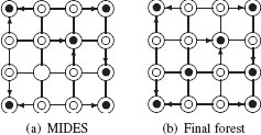
FIGURE 11.12
A MIDES built on a 4 × 4 grid.

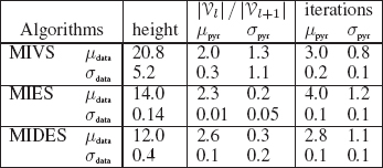
TABLE 11.1
Statistics on height of the pyramid, decimation ratio, and number of iterations.

•  Step II. Define the target of each tree of the resulting forest as a survivor and the sources as nonsurviving vertices attached to this unique target;

•  Step III. Complete this forest with isolated vertices.

Note that, contrary to the MIES (Section 11.3.4), the MIDES construction scheme does not require us to split existing trees in order to obtain trees of depth one. Kropatsch et al. [12] have shown that the decimation ratio obtained by a MIDES is at least 2.0 if the MIDES does not produce isolated vertices. Experiments performed in the same paper show that such isolated vertices do not occur frequently. Moreover, each isolated vertex needs only one tree of more edges to keep the balance for a reduction factor of 2.0.

11.3.6  Comparison of MIVS, MIES, and MIDES

Kropatsch et al. [12] have compared the MIVS, MIES, and MIDES construction schemes of a pyramid through several experiments based on a database of pyramids computed on initial graphs encoding 100 × 100, 150 × 150, and 200 × 200, 4-connected planar grids. The outcome of the random variable used within the maximal independent set is repeated with different seeds in order to obtain up to 1000 different pyramids. Statistics of all pyramids built by each specific selection (MIVS, MIES, and MIDES) are calculated to compare the properties of the different strategies by using the following parameters:

•  The height of the pyramid (height)

•  The reduction factor for vertices $\left(\frac{\left|{\mathcal{V}}_l\right|}{\left|{\mathcal{V}}_{l+1}\right|}\right)$

•  The number of iterations required to complete a maximal independent set using repeated maxima selection of the outcome of a random variable (Section 11.3.2).

Note that the reduction factor and the number of iterations vary within a pyramid. We thus compute the mean (μ_pyr) and standard deviation (σ_pyr) of these values for each pyramid and further compute the mean (μ_data) and standard deviation (σ_data) of these global value over our whole dataset of pyramids. The resulting values are displayed in Table 11.1.

As shown by Table 11.1, MIVS provides a mean reduction factor equal to 2.0 but with an important standard deviation within the pyramid (1.3). This important variability of the decimation factor is coherent with the large mean height (20.8) of the pyramid. The maximal height on the dataset obtained using the MIVS being equal to 41. The mean number of iterations is stable (σ_pyr = 0.8) and equal to 3.0. In conclusion, MIVS provide a mean reduction factor of 2.0, but such a mean result hides bad behaviors of the MIVS which have large chances to occur.

Compared to the MIVS, the MIES provides a larger mean decimation ratio (2.3), this decimation ratio being stable along the pyramid (σ_pyr = 0.2). The mean height of the pyramid is also lower (14.0) with a much lower standard deviation (0.14). The maximal height of a pyramid obtained using the MIES construction scheme within these experiments is equal to 15. The mean number of iterations (4.0) is, however, greater than the one of MIVS (3.0) with also a larger standard deviation (1.2). In conclusions, MIES provides a more stable and larger decimation ratio than MIVS. Our observations of this decimation ration was greater than its theoretical bound (2.0) in all experiments.

The mean reduction factor obtained using the MIDES construction scheme (2.6) is the largest of the three methods with a low variation within pyramids (σ_pyr = 0.3). The mean height of the pyramid (12.0) is also lower than the one obtained with MIES and MIVS and remains stable across the database (σ_data = 0.4). The number of iterations needed to complete the maximal independent set is comparable with the one of MIVS. The MIDES thus provides both a large and stable reduction factor and a low number of iterations.

11.4  Irregular Pyramids and Image properties

Different families of irregular pyramids have been proposed [5, 15, 16] to encode image content. These pyramids may vary both according to the method used to build one graph of the pyramid from the graph below and according to the type of graph used to encode each level. The construction scheme of a pyramid, described in Section 11.3, determines its decimation ratio and may be understood as the pyramid’s vertical dynamic. Conversely, the choice of a given graph model determines which set of topological and geometrical image properties may be encoded at each level. This last choice may be understood as the determination of the horizontal resolution of the pyramid. Let us additionally note that choices concerning pyramid’s construction scheme and graph encoding are usually independent since different pyramid construction schemes may be applied using different graph encoding. The main geometrical and topological properties of an image together with the different graph models used to encode them within the irregular pyramid framework are detailed in the following sections.

11.4.1  Relating Regions

Within an image analysis scheme, a high level image description is usually based on low level image processing steps. The segmentation stage is one of this key step. Segmentation produces an image’s partition into meaningful connected sets of pixels called regions. However, in many applications, the low-level image segmentation stage cannot be readily separated from high-level goals. On the contrary, segmentation algorithms should often extract fine information about a partition in order to guide the segmentation process according to high level objectives. There is thus a need to design graph models which can be both efficiently updated during a segmentation stage and which may be used to extract fine information about the partition.

Region’s adjacency also called meet relationship constitutes a basic but widely used relationship between regions. Two regions of a partition are said to be adjacent if they share at least one common boundary segment. Figure 11.13(a) shows a partition of an 8 × 8 image whose boundaries are displayed in Figure 11.13(b) using interpixels elements such as linels (or cracks) and pointels [17, 18]. One may see from these figures that the meet relationship corresponds to different configurations of regions. For example, the central gray region G contains a black region B₂ and shares one common boundary segment with another black region B₁. In the same way, white and black regions, W on the left and B₁ on the right part of the image, respectively, share two connected boundaries.

Finer relationships between regions such as RCC-8 defined by Randel [19] or the relationships defined by K. Shearer et al. [20] in the context of graph matching should thus be used in order to describe fine relationships between regions. Within the particular context of image segmentation, the following relationships may be defined from these two models:

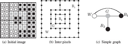
FIGURE 11.13
An image partition (a) whose boundaries are encoded by interpixel elements (b). A simple graph encoding of the resulting partition (c).

Meets: The different models used to encode partitions either encode the existence of at least one common boundary segment between two region or create one relationship for each boundary segment between these regions. We denote these two types of encoding meets_exists and meets_each. A model encoding only the meets_exists relationship is thus not able to distinguish a simple from a multiple adjacency relationship between two regions such as the one between vertices W and B₁ in Figure 11.13. Note that the ability of models to retrieve efficiently a given common boundary segment between two regions is also an important feature of these models;

Contains: The relationship A contains B expresses the fact that region B is completely surrounded by region A. For example, the gray region G in Figure 11.13(a) contains the black region B₂;

Inside: The inside relationship is the inverse of the contains relation: The region B₂ inside G is contained in G.

One additional relationship not directly handled by Shearer and Randel’s models may be defined within the hierarchical segmentation scheme. Indeed, within such a framework a region defined at a given level of a hierarchy is composed of regions defined at levels below.

The following relationships may thus be deduced from the relationships defined by Shearer and Randel and the example provided by Figure 11.13(a) : The meets_exists, meets_each, contains, inside and composed of. Note that unlike meets relationships, the contains and inside relations are asymmetric. Hence, contains or inside relation between two regions allows us to characterize each of the regions sharing this relation.

11.4.2  Graph models

Different graph models [21] have been proposed to describe the content of an image within the image analysis framework. Each of these graph models encodes a different subset of the relationships defined in Section 11.4.1. In the following sections, we present the main graph models introduced within the irregular pyramid framework together with a description of the relationships between regions encoded by such models.

11.4.2.1  Simple Graph

One of the most common graph data structure, within the segmentation, framework is the region adjacency graph. A RAG is defined from a partition by associating one vertex to each region and by creating an edge between two vertices if the associated regions share a common boundary segment (Figure 11.13(c)). A RAG thus encodes the meet_exists relationship. It corresponds to a simple graph without any double edge between vertices nor self-loop. The simplification of a RAG is based on the following graph transformations:

Edge removal: The removal of an edge from a graph $\mathcal{G}=\left(\mathcal{V},ℰ\right)$ consists to remove it from $ℰ$. In order to avoid to disconnect the graph, removed edges should not define a bridge.

Edge contraction: The contraction of an edge consists to collapse the two vertices incident to the edge into a single vertex and to remove the edge. Self-loops are excluded from edge contraction since both end points correspond to a same point which cannot collapse with itself.

The contraction operation is defined for any edge except self-loops and thus for any set of edges which does not contain a cycle (i.e., a forest). Given a graph $\mathcal{G}=\left(\mathcal{V},ℰ\right)$ and a set $\mathcal{N}\subset ℰ$ defining a forest of $\mathcal{G}$, the contraction of $\mathcal{N}$ in $\mathcal{G}$ is denoted $\mathcal{G}/\mathcal{N}$. In a similar way, given a set $ℳ$ of edges, the removal of $ℳ$ in $\mathcal{G}$ is denoted by $\mathcal{G}ℳ$. In order to preserve the connectedness of G, $ℳ$ should not correspond to a cut-set.

Within a non-hierarchical segmentation scheme the RAG model is usually applied as a merging step to overcome the oversegmentation produced by a previous splitting algorithm. Indeed, the existence of an edge between two vertices denotes the existence of at least one common boundary segment between the two associated regions which may thus be merged by removing this segment. Within this framework, edge information may thus be interpreted as a possibility to merge two regions identified by the vertices incident to the edge. This merging operation of two adjacent vertices is encoded within the RAG model by the contraction of the edge encoding their adjacency. This contraction has to be followed by a removal step in order to keep the graph simple by removing all multiple edges or self-loops which may have been created by the contraction operation.

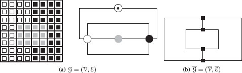
FIGURE 11.14
A nonsimple graph encoding a partition (a) and its dual (b).

The RAG model thus encodes only the existence of a common edge between two regions (the meets_exists relationship). Moreover, the existence of a common edge between two vertices does not provide enough information to differentiate a meets relationship from a contains or inside one. This drawback is illustrated in Figure 11.13(c) where the relationships between G and B₁ is the same than the one between G and B₂ (both B₁ and B₂ are adjacent to G). However, the gray region associated to G contains the black region associated to B₂ but just shares one connected boundary segment with the black region encoded by B₁. These two different configurations of regions are not differentiated by the simple graph model.

11.4.2.2  Dual Graph Model

Edges within a RAG model only encode the meet_exists relationship. One straightforward solution to encode multiple boundaries between regions consists in creating one edge between two vertices for each common boundary segment between the two corresponding regions. The resulting graph is nonsimple. The set of vertices $\mathcal{V}$ and of edges $ℰ$ of such a graph $\mathcal{G}=\left(\mathcal{V},ℰ\right)$ is defined by the following requirements:

•  Req. I. Each vertex of $\mathcal{V}$ encodes a region of the image, one additional special vertex encodes the background of the image

•  Req. II. Each edge of $ℰ$ encodes a maximal connected boundary segment between two connected components.

Figure 11.14(a) shows such an encoding where the two connected boundaries between black and white regions are encoded by two edges between the corresponding vertices. Vertex (⨀) encodes the background of the image. White and black regions being adjacent to the background, vertices encoding these regions are adjacent to the vertex encoding the background. Such a graph encoding does not allow us to readily perform graph simplifications. This last drawback is illustrated in Figure 11.15(b) whose graph is obtained by contracting the edge between dark gray (●) and white (○) vertices defined in Figure 11.15(a). This edge contraction operation induces the merge of the corresponding regions in Figure 11.15(a) hence producing a partition similar to the one displayed in Figure 11.14(a). As illustrated in Figure 11.15(b), edge contraction between dark gray and white vertices induces the creation of two edges between white and gray vertices. These two edges encode a single boundary segment between the white and gray regions and should thus be merged into a single one. However, the use of a single graph does not allow us to readily distinguish these two edges from the double edges between white and black vertices which encode two nonconnected boundaries and should thus be preserved by any simplification step. Note that the same redundancy problem occurs for the two edges encoding adjacency relationships between the white (○) and background (⨀) vertices.

The dual graph model proposed by Kropatsch [22] allows us to perform efficient simplifications of nonsimple graphs after a set of edge contractions. This model assumes that objects to be modeled lie in the 2D plane and may thus be encoded by a connected planar graph. Using this assumption, the dual graph model is defined as a couple of connected dual graphs $\left(\mathcal{G},\overline{\mathcal{G}}\right)$, where $\mathcal{G}=\left(\mathcal{V},ℰ\right)$ is a nonsimple graph defined by Req. I (Section 11.4.2.2) and Req. II (Section 11.4.2.2) while $\overline{\mathcal{G}}$ is the dual of $\mathcal{G}$.

The dual graph of $\mathcal{G},\overline{\mathcal{G}}=\left(\overline{\mathcal{V}},\overline{ℰ}\right)$ is defined by creating one vertex (■, Figure 11.14(b)) of $\overline{\mathcal{G}}$ for each face of $\mathcal{G}$ and connecting these vertices such that each edge of $\mathcal{G}$ is crossed by one edge of $\overline{\mathcal{G}}$. Note that $\mathcal{G}$ may encode several edges between two vertices. It is thus a nonsimple graph. Its dual $\overline{\mathcal{G}}=\left(\overline{\mathcal{V}},\overline{ℰ}\right)$ being also nonsimple.

Each dual graph $\overline{\mathcal{G}}$ being deduced automatically from the primal graph $\mathcal{G}$, both graphs $\mathcal{G}$ and $\overline{\mathcal{G}}$ share important properties, which are recalled below:

1.  The dual graph operation is idempotent:$\overline{\overline{\mathcal{G}}}=\mathcal{G}$. This important property means that the dual operation does not induce any loss of information since the primal graph may be recovered from its dual. One graph and its dual thus encode the same information differently;

2.  Since each edge of $\overline{\mathcal{G}}$ crosses one edge of $\mathcal{G}$, there is a one-to-one correspondence between edges of $\mathcal{G}$ and $\overline{\mathcal{G}}$. Given a set $\mathcal{N}$ of edges, we will denote by $\overline{\mathcal{N}}$ the corresponding set of edges in $\overline{\mathcal{G}}$;

3.  The contraction of any forest $\mathcal{N}$ in the primal graph is equivalent to the removal of $\overline{\mathcal{N}}$ in its dual. In other words:

$\overline{\mathcal{G}/\mathcal{N}}=\overline{\mathcal{G}}\overline{\mathcal{N}};$

(11.12)

Note that since $\mathcal{N}$ does not contain any cycle, $\overline{\mathcal{N}}$ does not define a cut-set. The initial graph $\mathcal{G}$ being connected, both graphs $\mathcal{G}/\mathcal{N}$ and $\overline{\mathcal{G}}\overline{\mathcal{N}}$ remain connected and dual of each other.

4.  Application of the above equation to the dual graph $\overline{\mathcal{G}}$ instead of $\mathcal{G}$ leads to the following equation:

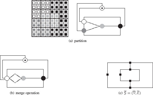
FIGURE 11.15
A partition into four regions and its associated nonsimple graph $\mathcal{G}$(a), the graph $\mathcal{G}$ obtained by the contraction of the edge between white and dark gray vertices. The dual graph of (b), $\overline{\mathcal{G}}=\left(\overline{\mathcal{V}},\overline{ℰ}\right)$ (c).

$\overline{\mathcal{G}}/\overline{\mathcal{N}}=\overline{\mathcal{G}\mathcal{N}}$

(11.13)

In other words, the contraction of any forest $\overline{\mathcal{N}}$ of $\overline{\mathcal{G}}$ is equivalent to the removal of $\mathcal{N}$ in $\mathcal{G}$.

As illustrated by Figure 11.15(b), edge contraction may induce the creation of some redundant edges. These edges belong to one of the following categories:

•  These edges encode multiple adjacency relationships between two vertices and define degree two faces. They can thus be characterized in the dual graph as degree two dual vertices (Figure 11.15(b and c)). In terms of a partition’s encoding these edges correspond to an artificial split of one boundary segment between two regions;

•  These edges correspond to a self-loop with an empty inside. These edges thus define degree one faces and are characterized in the dual graph as degree one vertices. Such edges encode artificial inner boundaries of regions.

Both redundant double edges and empty self-loops do not encode relevant topological relations and can be removed without any harm to the involved topology [22]. The resulting pair of dual graphs encodes each connected boundary segment between two regions by one edge between corresponding vertices. The dual graph model thus encodes the meets_each relationship through multiple edges between vertices.

FIGURE 11.16
The graph (b) defines the top of a dual graph pyramid encoding an ideal segmentation of (a). The self loop incident to vertex A may surround either vertex B or C without changing the incidence relations between vertices and faces. The dual vertices associated to faces are represented by filled boxes (■). Dual edges are represented by dashed lines.

Within the dual graph model, the encoding of the adjacency between two regions one inside the other is encoded by two edges (Figure 11.16): One edge encoding the common border between the two regions and one self-loop incident to the vertex encoding the surrounding region. One may think to characterize the inside relationship by the fact that the vertex associated to the inside region should be surrounded by the self-loop. However, as shown by Figure 11.16(c), one may exchange the surrounded vertex without modifying the incidence relationships between both vertices and faces. Two dual graphs being defined by these incidence relationships one can thus exchange the surrounded vertex without modifying the encoding of the graphs. This last remark shows that the inside/contains relationships cannot be characterized locally within the dual graph framework.

11.4.2.3  Combinatorial Maps

Combinatorial maps and generalized combinatorial maps define a general framework that allows us to encode any subdivision of nD topological spaces orientable or nonorientable with or without boundaries. An exhaustive comparison of combinatorial maps with other boundary representations such as cell-tuples and quad-edges is presented in [23]. Recent trends in combinatorial maps apply this framework to the segmentation of 3D images [24, 25] and the encoding of hierarchies [16, 26, 27].

This section is devoted to 2D combinatorial maps that we simply call combinatorial maps. A combinatorial map may be seen as a planar graph encoding explicitly the orientation of edges around a given vertex. Figure 11.17 demonstrates the derivation of a combinatorial map from a plane graph $\mathcal{G}=\left(\mathcal{V},ℰ\right)$ (Figure 11.14(a)). First, edges of $ℰ$ are split into two half edges called darts, each dart having its origin at the vertex it is attached to. The fact that two half edges (darts) stem from the same edge is recorded in the permutation α. A second permutation σ encodes the set of darts encountered when turning counterclockwise around a vertex. A combinatorial map is thus defined by a triplet $\mathcal{G}=\left(\mathcal{D},\sigma ,\alpha \right)$, where $\mathcal{D}$ is the set of darts and σ, α are two permutations defined on $\mathcal{D}$ such that α is an involution:

$\forall d\in \mathcal{D}{\alpha }^2\left(d\right)=d$

(11.14)

If darts are encoded by positive and negative integers, involution α may be implicitly encoded by the sign (Figure 11.17(b)).

Given a dart d and a permutation π, the π-cycle of d denoted by π*(d) is the series of darts ${\left({\pi }^i\left(d\right)\right)}_{i\in \mathbb{N}}$ defined by the successive applications of π on the initial dart d. The σ- and α-cycles of a dart d are thus, respectively, denoted by σ*(d) and α*(d).

The σ-cycle of one vertex encodes its adjacency relationships with neighboring vertices. For example, let us consider the dart 5 in Figure 11.17(b) attached to the white vertex. Turning counterclockwise around this vertex, we encounter the darts 5, −1, 6, and −3. We thus have σ(5) = −1, σ(−1) = 6, σ(6) = −3, and σ(−3) = 5. The σ-cycle of 5 is thus defined as σ*(5) = (5, −1, 6, −3). The whole permutation σ is defined as the composition of its different cycles and is equal to σ = (5, −1, 6, −3) (4, 3) (−5, −4, −6, −2) (1, 2). Permutation α being implicitly encoded by the sign in Figure 11.17, we have α*(5) = (5, −5) and α = (1, −1)(2, −2) …(6, −6).

We can already state one major difference between a combinatorial map and an usual graph encoding of a partition. Indeed, a combinatorial map may be seen as a planar graph with a set of vertices (the cycles of σ) connected by edges (the cycles of α). However, compared to an usual graph encoding, a combinatorial map encodes additionally the local orientation of edges around each vertex, thanks to the order defined within each cycle of σ.

Given a combinatorial map $\mathcal{G}=\left(\mathcal{D},\sigma ,\alpha \right)$, its dual is defined by $\overline{\mathcal{G}}=\left(\mathcal{D},\phi ,\alpha \right)$ with φ = σ ∘ α. The cycles of the permutation φ encode the sequence of darts encountered when turning around a face of G. Note that, using a counterclockwise orientation for permutation σ, each dart of a φ-cycle has its associated face on its right (see, e.g., the φ-cycle φ* (5) = (5, −4, 3) in Figure 11.17(b)). Cycles of φ may alternatively be interpreted as the sequence of darts encountered when turning clockwise around each dual vertex (Figure 11.17(c)). Permutation φ, on this last figure, being defined as φ = (−1, 2, −5)(5, −4, 3)(4, −6, −3)(1, 6, −2).

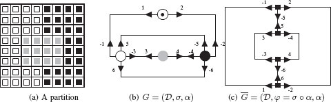
FIGURE 11.17
A partition (a) encoded by a combinatorial map (b) and its dual (c).

Each connected boundary segment between two regions is encoded by one edge within the combinatorial map formalism. Models based on combinatorial maps thus encode the meets_each relationship. However, within the combinatorial map framework, two connected components S inside R of a partition will be encoded by two combinatorial maps without any information about the respective positioning of S and R. Models based on combinatorial maps have thus designed additional data structure like list of contours [28], inclusion tree [29], or parent-child relationships [30, 18] to encode contains and inside relationships. These additional data structures should be closely related to the combinatorial map model in order to update both models when a partition is modified.

11.4.3  Simple Graph Pyramids

Simple graph pyramids are defined as a stack of successively reduced simple graphs, each graph being built from the graph below by selecting a set of vertices named surviving vertices and mapping each nonsurviving vertex to a survivor [8, 5]. Using such a framework, the graph ${\mathcal{G}}_{l+1}=\left({\mathcal{V}}_{l+1},{ℰ}_{l+1}\right)$ defined at level l + 1 is deduced from the graph defined at level l by the following steps:

1.  Define a partition of ${\mathcal{V}}_l$ into connected reduction windows and select one surviving vertex within each reduction window. Surviving vertices define the set ${\mathcal{V}}_{l+1}$ while nonsurviving vertices of each reduction windows are adjacent to the unique survivor of the reduction window (Section 11.3);

2.  Define adjacency relationships between vertices of ${\mathcal{G}}_{l+1}$ in order to define ${ℰ}_{l+1}$.

The selection of surviving vertices and the definition of a partition of ${\mathcal{V}}_l$ into reduction windows is described in Section 11.3. Note that the attachment of each nonsurviving vertex to the unique survivor of its reduction window induces a parent/child relationship between ${\mathcal{V}}_l$ and ${\mathcal{V}}_{l+1}$. Each nonsurviving vertex is the child of the unique survivor of its reduction window. Conversely, any surviving vertex is the parent of all nonsurviving vertices within its reduction window.

We are thus here mainly concerned with the second and last step of the decimation process that consists to connect surviving vertices in ${\mathcal{G}}_{l+1}$ in order to define ${ℰ}_{l+1}$. Meer [8] attaches the outcome of a random variable to each vertex and defines a partition of ${\mathcal{V}}_l$ into reduction windows using the maximal independent vertex set (MIVS) construction scheme (Section 11.3.2). Figure 11.18(a) (see also Figure 11.9) shows a decomposition of a 4 × 4, 8-connected grid into 4 reduction windows using such a construction scheme. Surviving vertices are marked by an extra circle, and reduction windows are superimposed to the figure. Given this decomposition of ${\mathcal{V}}_l$ into reduction windows, Meer joins two parents by an edge if they have adjacent children (e.g., vertices labeled 10 and 7 on the right side of Figure 11.18(a)). Since each child is attached directly to its parent, two adjacent parents at the reduced level are connected in the level below by paths of length less than or equal to three. Let us call these paths connecting paths. The set of edges ${ℰ}_{l+1}$ induced by connecting paths between surviving vertices in Figure 11.18(a) is shown in Figure 11.18(b).

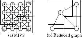
FIGURE 11.18
The reduced graph (b) deduced from the maximal independent vertex set (a) together with reduction windows superimposed to (b).

Two surviving vertices are thus connected in ${\mathcal{G}}_{l+1}$ if they are connected in ${\mathcal{G}}_l$ by a path of length lower or equal than 3. Two reduction windows adjacent by more than one such path will thus be connected by a single edge in the reduced graph. The stack of graphs produced by the above decimation process is thus a stack of simple graphs each simple graph encoding only the existence of one common boundary segment between two regions (the meets_exists relationship). Moreover, as mentioned in Section 11.4.2, the RAG model that corresponds to a simple graph does not allow us to encode contains and inside relationships.

Let us finally note that the above construction scheme of the reduced graph ${\mathcal{G}}_{l+1}=\left({\mathcal{V}}_{l+1},{ℰ}_{l+1}\right)$ from ${\mathcal{G}}_l=\left({\mathcal{V}}_l,{ℰ}_l\right)$ may be adapted to all parallel reduction schemes detailed in Section 11.3. Using different reduction schemes than the MIVS, it may be interesting to note that the construction of ${\mathcal{G}}_{l+1}$ from ${\mathcal{G}}_l$ may be equivalently performed by merging all the vertices of each reduction window into a single vertex (Section 11.4.2.1). This operation may be decomposed as follows:

1.  The selection of an unique edge between each nonsurviving vertex and its parent

2.  The contraction of the set of edges previously selected

3.  The removal of any double edge or self-loop that may have been created by the previous step.

Note, that MIES (Section 11.3.4) and MIDES (Section 11.3.5) construction schemes explicitly connect each nonsurviving vertex to its parent, hence providing the first step of the above process.

11.4.4  Dual Graph Pyramids

As mentioned in Section 11.4.3, the construction of each level of a simple graph pyramid may be decomposed into a contraction step, followed by the removal of any multiple edge or self-loop. Since each edge to be contracted connects a nonsurviving vertex to its surviving parent, the set $\mathcal{C}\mathcal{K}$ of contracted edges defines a forest of $\mathcal{C}\mathcal{K}$.

11.4.4.1  Contraction Kernel

The different parallel construction schemes of irregular pyramids presented in Section 11.3 allow us to define different forests $ℱ$ composed of trees of depth at most one hence allowing an efficient parallel contraction of each reduction window.

Kropatsch [3] proposed to abstract the set of edges to be contracted through the notion of contraction kernel. A contraction kernel is defined on a graph $\mathcal{G}=\left(\mathcal{V},ℰ\right)$ by a set of surviving vertices $\mathcal{S}$, and a set of nonsurviving edges $\mathcal{C}\mathcal{K}$ (shown as bold lines in Figure 11.19) such that:

•  $\mathcal{C}\mathcal{K}$ is a spanning forest of $G$;

•  Each tree of $\mathcal{C}\mathcal{K}$ is rooted by a vertex of $\mathcal{S}$.

Since the set of nonsurviving edges $\mathcal{C}\mathcal{K}$ forms a forest of the initial graph, no selfloop may be contracted and the contraction operation is well defined. The decimation of a graph by contraction kernels differs from the one defined in Section 11.4.3 on the two following points:

•  First, using contraction kernels, the set of surviving vertices is not required to form a MIVS. Therefore, two surviving vertices may be adjacent in the contracted graph;

•  Secondly, using contraction kernels a nonsurviving vertex is not required to be directly linked to its parent but may be connected to it by a branch of a tree (see Figure 11.19(a)). The set of children of a surviving vertex may thus vary from a single vertex to a tree with any depth.

Let us note that the reduction of a graph by a sequence of contraction kernels $\mathcal{C}{\mathcal{K}}_1,\dots ,\mathcal{C}{\mathcal{K}}_n$ composed of trees of depth one is equivalent to the application of one single contraction kernel $\mathcal{C}\mathcal{K}$ called the equivalent contraction kernel on the initial graph [31]. The set of edges of $\mathcal{C}\mathcal{K}$ is defined as the union of all edges of the contraction kernels ${\left(\mathcal{C}{\mathcal{K}}_i\right)}_{i\in \left\{1,\dots ,n\right\}}$. Conversely, any contraction kernel may be decomposed into a sequence of contractions kernels composed of trees of depth one. Contraction kernels should thus be understood as an abstraction of the forest of trees of depth one defined in Section 11.3. Conversely, methods presented in Section 11.3 provide practical heuristics to build contraction kernels fulfilling different properties.

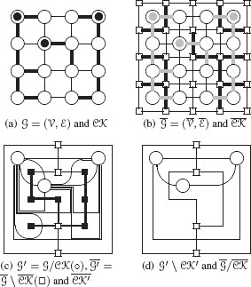
FIGURE 11.19
A contraction kernel $\left(\mathcal{S},\mathcal{C}\mathcal{K}\right)$ composed of three trees. Vertices belonging to $\mathcal{S}$ are marked with a filled circle inside(●). Dual vertices incident to redundant dual edges are shown as filled boxes (■).

Figure 11.19(a) illustrates a contraction kernel K composed of 3 trees drawn by thick lines (▬). The root of each tree being marked by dot circles (⨀).

This kernel is defined on a graph $\mathcal{G}$ encoding a 4 × 4 planar sampling grid. The dual of $\mathcal{G}$ is shown in Figure 11.19(b) together with the set of dual edges $\overline{\mathcal{C}\mathcal{K}}$. The graph $\mathcal{G}$ is superimposed to $\overline{\mathcal{G}}$ in order to highlight relationships between $\mathcal{C}\mathcal{K}$ and $\overline{\mathcal{C}\mathcal{K}}$. Contraction of $\mathcal{C}\mathcal{K}$ in $\mathcal{G}$ is equivalent to the removal of $\overline{\mathcal{C}\mathcal{K}}$ in $\overline{\mathcal{G}}$ (equation 11.12, Section 11.4.2). The resulting pair of reduced graph $\left(\mathcal{G}/\mathcal{C}\mathcal{K},\overline{\mathcal{G}}\overline{\mathcal{C}\mathcal{K}}\right)$ is shown in Figure 11.19(c).

As mentioned in Section 11.4.2, the contraction of a set of edges may create redundant edges such as double edges surrounding degree 2 faces and self-loops corresponding to degree one faces. These redundant edges may be efficiently characterized in the dual graph, respectively, as degree 2 and degree 1 dual vertices. Such redundant dual vertices are shown in Figure 11.19(c) as filled boxes (∎). Removal of degree one dual vertices may be achieved by contracting the only edge incident to such vertices. In the same way, degree 2 dual vertices may be removed by contracting one of their incident edge. The resulting set of edges $\overline{\mathcal{C}{\mathcal{K}}^{\prime }}$ defines a forest of the dual graph $\overline{\mathcal{G}}$ and is called a removal kernel (thick edges (−) in Figure 11.19(c)). Indeed, contraction of $\overline{\mathcal{C}{\mathcal{K}}^{\prime }}$ in $\overline{\mathcal{G}}$ is equivalent to the removal of $\mathcal{C}{\mathcal{K}}^{\prime }$ in $\mathcal{G}$ (Section 11.4.2). The reduction of a dual graph $\left(\mathcal{G},\overline{\mathcal{G}}\right)$ is thus performed in two steps:

•  A first contraction step that computes $\left({\mathcal{G}}^{\prime },\overline{{\mathcal{G}}^{\prime }}\right)=\left(\mathcal{G}/\mathcal{C}\mathcal{K},\overline{\mathcal{G}}\mathcal{C}\mathcal{K}\right)$ from $\left(\mathcal{G},\overline{\mathcal{G}}\right)$ (Figure 11.19(a-c));

•  The definition of a removal kernel $\overline{\mathcal{C}{\mathcal{K}}^{\prime }}$ from $\left({\mathcal{G}}^{\prime },\overline{{\mathcal{G}}^{\prime }}\right)$ that removes all redundant double edges and empty self-loops of $\mathcal{G}$ by computing $\left({\mathcal{G}}^{\prime }\mathcal{C}{\mathcal{K}}^{\prime },\overline{{\mathcal{G}}^{\prime }}/\mathcal{C}{\mathcal{K}}^{\prime }\right)$ (Figure 11.19(d)).

A dual graph pyramid introduced by Kropatsch [3] is defined as a stack of pairs of dual graphs $\left(\left({\mathcal{G}}_0,\overline{{\mathcal{G}}_0}\right),\dots ,\left({\mathcal{G}}_n,\overline{{\mathcal{G}}_n}\right)\right)$, successively reduced. Each graph ${\mathcal{G}}_{i+1}$ is deduced from ${\mathcal{G}}_i$ by a contraction kernel $\mathcal{C}{\mathcal{K}}_i$ followed by the application of a removal kernel removing any redundant double edge or empty self loop that may have been created by the contraction step. The initial graph ${\mathcal{G}}_0$ and its dual $\overline{{\mathcal{G}}_0}$ may encode a planar sampling grid or be deduced from an oversegmentation of an image.

11.4.4.2  Dual Graph pyramids and Topological relationships

Given one tree of a contraction kernel, the contraction of its edges collapses all the vertices of the tree into a single vertex and keeps all the connections between the vertices of the tree and the remaining vertices of the graph. The multiple boundaries between the newly created vertex and the remaining vertices of the graph are thus preserved. Each graph of a dual graph pyramid thus encodes the meets_each relationships. This property is not modified by the application of a removal kernel that only removes redundant edges.

Moreover, due to the forest requirement, the encoding of the adjacency between two regions one inside the other is encoded by two edges (Figure 11.16): One edge encoding the common border between the two regions and one self-loop incident to the vertex encoding the surrounding region. As mentioned in Section 11.4.2.2 (Figure 11.16), such a couple of edges does not allow to characterize locally contains and inside relationships.

11.4.5  Combinatorial Pyramids

As in the dual graph pyramid scheme [32] (Section 11.4.4), a combinatorial pyramid is defined by an initial combinatorial map successively reduced by a sequence of contraction or removal operations. The initial combinatorial map encodes a planar sampling grid or a first segmentation, and the remaining combinatorial maps of a combinatorial pyramid encode a stack of image partitions successively reduced. As mentioned in Section 11.4.2, page 330, a combinatorial map may be understood as a dual graph with an explicit encoding of the orientation of the edges incident to each vertex. This explicit encoding of the orientation is preserved within the combinatorial pyramid framework [33].

Contraction operations are controlled by contraction kernels (CK) defined as an acyclic set of darts encoding the set of edges to be contracted. Given a combinatorial map $\mathcal{G}=\left(\mathcal{D},\sigma ,\alpha \right)$, a kernel $\mathcal{C}\mathcal{K}$ defined on $\mathcal{G}$ is thus included in $\mathcal{D}$ and symmetric according to α:

$\forall d\in \mathcal{C}\mathcal{K},\alpha \left(d\right)\in \mathcal{C}\mathcal{K}$

(11.15)

The removal of redundant edges is performed as in the dual graph reduction scheme by a removal kernel. Such kernels are, as contraction kernels, defined as sets of darts to be deleted. Contrary to the dual graph pyramid framework, removal kernels are decomposed in two subkernels: A removal kernel of empty self-loops (RKESL) which contains all darts incident to a degree 1 dual vertex and a removal kernel of empty double edges (RKEDE) which contains all darts incident to a degree 2 dual vertex. These two removal kernels are defined as follows: The removal kernel of empty selfloops RKESL is initialized by all self-loops surrounding a dual vertex of degree 1. RKESL is further expanded by all self-loops that contain only other self-loops already in RKESL until no further expansion is possible. For the removal of empty double edges RKEDE, we ignore all empty self-loops in RKESL in computing the degree of the dual vertex.

Note that the removal of degree two dual vertices by a RKEDE may be achieved using two distinct operations illustrated in Figure 11.20. A first solution (Figure 11.20(b)) consists to remove all darts incident to a degree two vertex. This solution implies to update involution α at each level of the pyramid but simplifies the modification that may affect a dual vertex since a dart remains incident to a same dual vertex until it is removed by some contraction or removal operation. Conversely, the second solution (Figure 11.20(c)) keeps involution α constant but may change the attachment of a dart to a dual vertex. Both encoding of a RKEDE define valid combinatorial pyramids and we choose the first solution for the remaining of this chapter.

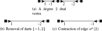
FIGURE 11.20
The dual vertex of degree 2, φ*(−1) = (−1, 2) (a) may be suppressed by removing darts −1 and 2 that define the degree 2 dual vertex (b). Permutation α should then be updated as α’(1) = −2 and α’(−2) = 1. This dual vertex may be alternatively removed by contracting in the dual graph one of the two edges incident to this dual vertex. The contracted edge (2, −2) is removed in (c). Involution α remains unchanged in this case, but the contraction operation has replaced −2 by −1 within the φ cycle encoding the right vertex, hence modifying the dual vertex to which dart −1 is attached to.

The successive application of a RKESL and a RKEDE may be encoded as the application of a single removal kernel. However, this decomposition allows us to distinguish darts encoding boundaries between two regions from inner boundaries within the implicit encoding scheme of combinatorial pyramids (next section). Both contraction and removal operations defined within the combinatorial pyramid framework are thus defined as in the dual graph framework but additionally preserve the orientation of edges around each vertex. Further details about the construction scheme of a combinatorial pyramid may be found in [16].

11.4.5.1  Relationships between regions

Concerning the encoding of relationships between regions, combinatorial pyramids provide, as dual graph pyramids, an encoding of both meets_each and contains/inside relationships. This last relationship is encoded in both models by self-loops. A region R₁ inside a region R₂ being characterized by a self-loop incident to υ₂ (associated to R₂) and surrounding υ₁ (encoding R₁). However, using the dual graph framework, such configurations of vertices may be characterized only through global calculus over the whole graph. On the other hand, the explicit encoding of the orientation provided by combinatorial maps allows us to retrieve the set of regions inside a region encoded by a vertex υ in a time proportional to the degree of υ [27].

One may think to use the additional data structures (Section 11.4.2.3) defined within the combinatorial map framework to encode inside relationships within the combinatorial pyramid model. This solution would break the efficiency of the hierarchical data structure. Indeed, contains and inside relationships may be both created and removed within the pyramid. Therefore, the explicit encoding of these relationships by additional data structures would lead to associate to a pyramid a sequence of data structures whose size do not decrease between two successive levels of a pyramid. The overall size of each level of the pyramid may thus not decrease with a fixed rate or even increase, hence violating the main requirement of a hierarchical data structure (Section 11.3). Note that, conversely, the encoding of contains and inside relationships by self-loops is not adapted to the combinatorial map framework. Indeed, region splitting operations encoded within the combinatorial map model by the addition of edges may lead to cumbersome computations when these additional borders modify the contains/inside relationships encoded by self-loops. Such additions of edges that are not allowed within the combinatorial pyramid model are frequent within the nonhierarchical combinatorial map model. An explicit encoding of contains/inside relationships by additional data structures is thus preferred within this last model.

11.4.5.2  Implicit Encoding of a Combinatorial Pyramid

Let us consider an initial combinatorial map ${\mathcal{G}}_0=\left(\mathcal{D},\sigma ,\alpha \right)$ and a sequence of kernels $\mathcal{C}{\mathcal{K}}_1,\dots ,\mathcal{C}{\mathcal{K}}_n$ successively applied on ${\mathcal{G}}_0$ to build the pyramid. Each combinatorial map ${\mathcal{G}}_i=\left(\mathcal{S}{\mathcal{D}}_i,{\sigma }_i,{\alpha }_i\right)$ is defined from ${\mathcal{G}}_{i-1}=\left(\mathcal{S}{\mathcal{D}}_{i-1},{\sigma }_{i-1},{\alpha }_{i-1}\right)$ by the application of the kernel $\mathcal{C}{\mathcal{K}}_i$ on ${\mathcal{G}}_{i-1}$, and the set of surviving darts at level $i:{\mathcal{S}\mathcal{D}}_i$ is equal to $\mathcal{S}{\mathcal{D}}_{i-1}{K}_i$. We have thus:

$\mathcal{S}{\mathcal{D}}_{n+1}\subseteq \mathcal{S}{\mathcal{D}}_n\subseteq \dots \mathcal{S}{\mathcal{D}}_1\subseteq \mathcal{D}$

(11.16)

The set of darts of each reduced combinatorial map of a pyramid is thus included in the one of the base level combinatorial map. This last property allows us to define the two following functions:

1.  One function state from {1, …, n} to the states {CK, RKESL, RKEDE} that specifies the type of kernel applied at each level;

2.  One function level defined for all darts in $\mathcal{D}$ such that level (d) is equal to the maximal level where d survives:

$\forall d\in \mathcal{D}\text{level}\left(d\right)=\max \left\{i\in \left\{1,\dots ,n+1\right\}|d\in \mathcal{S}{\mathcal{D}}_{i-1}\right\}$

(11.17)

a dart d surviving up to the top level has thus a level equal to n + 1. Note that if $d\in \mathcal{C}{\mathcal{K}}_i,i\in \left\{1,\dots ,n\right\}$, then level(d) = i.

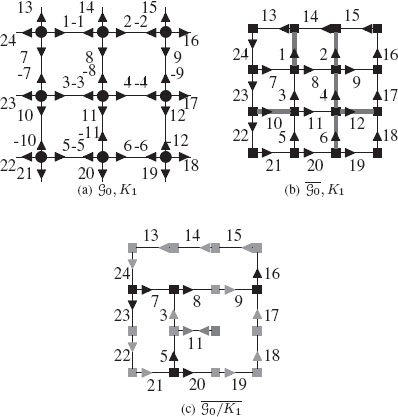
FIGURE 11.21
A combinatorial map (a) and its dual (b) encoding a 3 × 3 grid with the contraction kernel K₁ = α*(1, 2, 4, 12, 6, 10) (▬) superimposed to both figures. Only positive darts are represented in (b) and (c) in order to not overload them. The resulting reduced dual combinatorial map (c) should be further simplified by a removal kernel of empty self-loops (RKESL) K₂ = α*(11) to remove dual vertices of degree 1 (■). Dual vertices of degree 2 (■) are removed by the RKEDE K₃ = φ*(24, 13, 14, 15, 9, 22, 17, 21, 19, 18,) ∪ {3, −5}. Note that the dual vertex φ*(3) = (3, −5, 11) becomes a degree 2 vertex only after the removal of α*(11).

We have shown [16] that the sequence of reduced combinatorial maps ${\mathcal{G}}_0,\dots ,{\mathcal{G}}_{n+1}$ may be encoded without any loss of information using only the base level combinatorial map ${\mathcal{G}}_0$ and the two functions level and state. Such an encoding is called an implicit encoding of the pyramid. Figure 11.22(a) illustrates the implicit encoding of the pyramid defined in Figure 11.21 by an initial combinatorial map encoding a 3 × 3 grid and three kernels K₁, K₂, and K₃. These kernels defined at levels 1, 2, and 3 are, respectively, represented by red (►), green (►), and blue (►) darts in Figure 11.22(a).

The encoding of the function state being proportional to the height of the pyramid, its memory cost is negligible compared to the cost of the base level combinatorial map. The encoding of the function level requires us to associate one integer to each dart. The memory cost of such a function for a pyramid composed of n levels is thus equal to ${\log }_2\left(n\right)\left|\mathcal{D}\right|$. Using an implicit encoding of the involution α, the encoding of permutation σ requires $\left|\mathcal{D}\right|{\log }_2\left(\left|\mathcal{D}\right|\right)$ bytes. The total memory cost of an implicit pyramid is thus equal to:

$\left[{\log }_2\left(n\right)+{\log }_2\left(\left|\mathcal{D}\right|\right)\right]\left|\mathcal{D}\right|.$

(11.18)

On the other hand, using an explicit encoding of a combinatorial pyramid, if we suppose that the number of darts decreases by a factor 2 between each level, the total number of darts of the whole pyramid is equal to:

$\left|\mathcal{D}\right|{\displaystyle \sum _{i=0}^p\frac{1}{2^i}\approx 2\left|\mathcal{D}\right|}$

(11.19)

where $\left|\mathcal{D}\right|$ is supposed to be a power of $2\left(\left|\mathcal{D}\right|=2^p\right)$. The total memory cost of the explicit encoding of a combinatorial pyramid is thus equal to:

$2\left|\mathcal{D}\right|{\log }_2\left(\left|\mathcal{D}\right|\right).$

(11.20)

The ratio between Equations 11.18 and 11.20 is equal to:

$\frac{1}{2}\left(1+\frac{{\log }_2\left(n\right)}{{\log }_2\left(\left|\mathcal{D}\right|\right)}\right)$

(11.21)

The value of log₂ (n) being usually much lower than ${\log }_2\left(\left|\mathcal{D}\right|\right)$, the implicit encoding provides a lower memory cost than the explicit encoding. Let us additionally note that if we bound the maximal level of a pyramid using, for example, 32 bits integers to store the function level, we obtain a hierarchical encoding which is in practice independent of the height of the pyramid.

11.4.5.3  Dart’s Embedding and Segments

The receptive field of a dart $d\in \mathcal{S}{\mathcal{D}}_i$ corresponds to the set of darts reduced to d at level i [16]. Using the implicit encoding of a combinatorial pyramid, the receptive field RF_i(d) of $d\in \mathcal{S}{\mathcal{D}}_i$ is defined as a sequence d₁. …. d_q of darts in $\mathcal{D}$ such that d₁ = d, d₂ = σ₀(d) and for each j in {3, …, q} :

$d_j=\{\begin{array}{l}{\phi }_0\left(d_{j-1}\right)\text{if}\text{state}\left(\text{level}\left(d_{j-1}\right)\right)=CK\hfill \\ {\sigma }_0\left(d_{j-1}\right)\text{if}\text{state}\left(\text{level}\left(d_{j-1}\right)\right)\in \left\{RKEDE,RKESL\right\}\hfill \end{array}$

(11.22)

The dart d_q is defined as the last dart of the sequence that has been contracted or removed below the level i. Therefore, the successor of d_q according to Equation 11.22, d_q+1 satisfies level (d_q+1) > i. Moreover, we have shown [16] that d, d_q, and d_q+1 are additionally connected by the two following relationships:

${\sigma }_i\left(d\right)=d_{q+1}\text{and}{\alpha }_i\left(d\right)={\alpha }_0\left(d_q\right)$

(11.23)

Using a combinatorial map encoding of image content, regions and maximal connected boundaries between regions are, respectively, encoded by σ and α cycles. Therefore, each dart $d\in \mathcal{S}{\mathcal{D}}_i$ encodes a boundary segment between the regions associated to ${\sigma }_i^{\ast }\left(d\right)$ and ${\sigma }_i^{\ast }\left({\alpha }_i\left(d\right)\right)$. Moreover, in the lower levels of the pyramid, the two vertices of an edge may belong to a same region. We call the corresponding boundary segment an internal boundary in contrast to an external boundary that separates two different regions. The receptive field of d at level i (RF_i(d)) contains both darts corresponding to this boundary segment and additional darts corresponding to internal boundaries. The sequence of external boundary darts contained in RF_i(d) is denoted by ∂RF_i(d) and is called a segment. The order on ∂RF_i(d) is deduced from the receptive field RF_i(d). Given a dart $d\in \mathcal{S}\mathcal{D}$, the sequence ∂RF_i(d) = d₁, …, d_q is retrieved by [34]:

$d_1=d\text{and}\forall j\in \left\{1,\dots ,q-1\right\}{d}_{j+1}={\phi }_0^{n_j}\left({\alpha }_0\left(d_j\right)\right)$

(11.24)

The dart d_q is the last dart of ∂RF_i (d) that belongs to a double edge kernel. This dart is thus characterized using equation 11.23 by d_q = α₀ (α_i(d)). Note that each dart of the base level corresponds to an oriented crack [17, 18] (Section 11.4.2). A segment thus corresponds to a sequence of oriented cracks encoding a connected boundary segment between two regions [34].

The value n_j is defined for each j ∈ {1, …, q − 1} by:

$n_j=\min \left\{k\in {\mathbb{N}}^{\ast }|\text{state}\left(\text{level}\left({\phi }_0^k\left({\alpha }_0\left(d_j\right)\right)\right)\right)=RKEDE\right\}.$

(11.25)

A segment may thus be interpreted as a maximal sequence, according to Equation 11.24, of darts removed as double edges. Such a sequence connects two darts (d and α₀(d_q) = α_i(d)) surviving up to level i. The retrieval of the boundaries using equations 11.24 and 11.25 is one of the major reasons that lead us to distinguish empty self-loop and redundant double edges removal kernels. Let us additionally note that if ${\mathcal{G}}_0$ encodes the 4-connected planar sampling grid, each φ₀ cycle is composed of at most 4 darts (Figure 11.19(b)). Therefore, the computation of d_j+1 from d_j (Equation 11.24) requires at most 4 iterations and the determination of the whole sequence of cracks composing a boundary segment between two regions is performed in a time proportional to the length of this boundary.

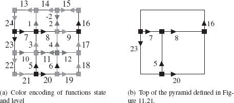
FIGURE 11.22
Implicit encoding (a) and top level combinatorial map (b) of the pyramid defined in Figure 11.21. Red, green and blue darts have level equal to 1, 2, and 3 respectively. States associated to these levels are, respectively, equal to CK, RKESL, RKEDE.

Let us consider the border of level 3 associated to dart 16 in Figure 11.22. According to Equation 11.24, 16 is the first dart of ∂RF₃ (16). Moreover, φ₀(α₀(16)) = φ₀(–16) = 15 belongs the RKEDE K₃ (Figure 11.22(a)). We have thus n₁ = 1 (Equation 11.25), and the second dart d₂ of ∂RF₃(16) is equal to 15. Using once again Equation 11.24, d₃ is the first dart encountered from φ₀(α₀(15)) by iterating permutation φ₀. Since φ₀((α₀(15)) = φ₀(−15) = −2 is a contracted dart, we should iterate permutation φ₀ at least one more time. The dart ${\phi }_0^2\left(\left({\alpha }_0(15\right)\right)={\phi }_0\left(-2\right)=14$ belongs to the RKEDE K₃, and we have thus n₂ = 2 and d₃ = 14. Further iterations of Equations 11.24 and 11.25 lead to the sequence:

$\partial R{F}_3\left(16\right)=\mathrm{16.15.14.13.24}$

(11.26)

which encodes the border between the first line of the image and the background.

In conclusion, the implicit encoding of a combinatorial pyramid provides an efficient encoding of the pyramid with a low memory cost and an efficient access to the geometry of segments defining the image’s partition.

Figure 11.23 illustrates an application of combinatorial pyramids to image segmentation. The gradient of the original image (Figure 11.23(a)) is encoded by a planar sampling grid encoded by a combinatorial map. Each edge of such a combinatorial map is valuated by a gradient measure between its two incident pixels [35]. The encoding of a watershed transform on this combinatorial map is performed by computing a contraction kernel whose each tree spans a watershed’s basin. The application of such a contraction kernel to obtain Figure 11.23(b) may be performed sequentially or using any parallel method defined in Section 11.3. Each edge of this partition is valuated by a relevance measure encoded by gray levels in Figure 11.23(c). This measure of relevance is based on edge’s dynamic and is computed using the profile of the gradient along each segment [26]. Such a measure is thus based on the computation of the external boundary of each dart. Finally, further levels of the pyramid are computed from Figure 11.23(c) by merging least relevant edges and updating the remaining edge’s relevance at each step. Such a strategy uses the implicit encoding of combinatorial maps in order to reduce memory requirements. The last level of the pyramid before a wrong merge operation is performed on Lena’s hat is displayed Figure 11.23(d).

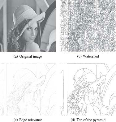
FIGURE 11.23
An application of combinatorial pyramid to hierarchical image segmentation.

11.5  Conclusion

Graphs have become a representational tool to bridge the gap between the raw information sources provided by sensors and the highly complex structure of the sensed world and the knowledge about it. A typical example is a digital image: it is the projection of the world’s structure and geometry into the image plane where some instances and basic objects can be observed together with certain properties like brightness or color and object-to-object relations like adjacency or closeness.

Embedded attributed graphs and combinatorial maps capture such low level visual cues and allow the aggregation of larger pieces of information that needs to be connected with the overall knowledge about the world. Both the sensed data and the high-level knowledge appear in huge amounts, and their processing is often of high complexity. In order to achieve the necessary efficiency hierarchies in different forms can be used.

This chapter introduced both regular and irregular pyramid frameworks connecting the embedded pixel arrangement with mid- and high-level abstraction hierarchies. Both frameworks allow us to efficiently analyze the content of an image using parallel calculus. Compared to non hierarchical methods, regular and irregular pyramids additionally provide a hierarchical description of the image’s content. Several drawbacks of regular pyramids, forbidding their use as a general framework for image analysis, lead to the definition of irregular pyramids. Such pyramids may be defined both by their construction scheme and by the graph model used within the pyramid.

We have presented the main parallel reduction schemes of irregular pyramids in Section 11.3. These construction schemes are based on the notion of independent sets defined on different parts of a graph according to each construction scheme. As mentioned by Table 11.2 (first column), the MIES and MIDES frameworks provide a theoretical bound on the height of the pyramid, while MIVS and D3P do not. All reduction schemes described in Section 11.3, but the D3P are based on the notion of maximal independent set (Table 11.2, second column). These last methods may be further classified according to the elements on which the maximal independent set is computed (Table 11.2, third column).

	Theoretical bound of pyramid’s height	Maximal independent set	Independent set on
MIVS	✗	✓	Vertices
D3P	✗	✗	Vertices
MIES	✓	✓	Undirected edges
MIDES	✓	✓	Directed edges

TABLE 11.2
Main positive (✓) and negative (✗) properties of parallel irregular pyramid construction schemes.

This chapter concludes on a presentation of the main type of graphs used within the irregular pyramid framework. Each graph model determines which type of image features may be encoded at each level of a pyramid. This choice of a graph model thus determines the range of image’s features that may be efficiently used by an image analysis or segmentation method and is hence an important parameter of such methods. As indicated in Table 11.3 (first column), all graph models encode the existence of a common boundary between two regions (meets_exists relationship). However, the explicit encoding of connected boundaries between regions is only provided by models based on dual graphs and combinatorial maps (table 11.3, second column). Contains and inside relationships are not encoded by models based on simple graphs. We expect that computing such relationships using the dual graph model requires global calculus on the whole graph. On the other hand, contains and inside relationships are explicitly encoded by additional data structures within the combinatorial map framework and may be efficiently computed by local calculus using combinatorial pyramids (Table 11.3, third column). Finally, the composed of relationship is only encoded by hierarchical models.

	meets_exists	meets_each	contains/inside	Composed of
RAG	✓	✗	✗	✗
Combinatorial maps	✓	✓	✓	✗
Simple graph pyramids	✓	✗	✗	✓
Dual graph pyramids	✓	✓	Global calculus?	✓
Combinatorial pyramids	✓	✓	Local calculus	✓

TABLE 11.3
Relationships available(✓) or not available (✗) using models described in this chapter.

This study of embedded hierarchical graph structures is probably only the first step to understand the complex strategies enabling humans to understand their environment and to react in real time. Further directions of research consider substructures invariant with respect to certain types of operations: topological structures invariant to continuous deformations [36]; or temporal structures capturing the components of a moving object [37, 38]; or generalizations being invariant to certain less relevant distictions of a class of objects enabling the focus on the main properties of the class.

Bibliography

[1]  P. Burt, T.-H. Hong, and A. Rosenfeld, “Segmentation and estimation of image region properties through cooperative hierarchial computation,” IEEE Transactions on Systems, Man and Cybernetics, vol. 11, no. 12, pp. 802–809, December 1981.

[2]  M. Bister, J. Cornelis, and A. Rosenfeld, “A critical view of pyramid segmentation algorithms,” Pattern Recognition Letter., vol. 11, no. 9, pp. 605–617, September 1990.

[3]  W. G. Kropatsch, “From equivalent weighting functions to equivalent contraction kernels,” in Digital Image Processing and Computer Graphics (DIP-97): Applications in Humanities and Natural Sciences, E. Wenger and L. I. Dimitrov, Eds., vol. 3346. SPIE, October 1997, pp. 310–320.

[4]  A. Rosenfeld and C.-Y. Sher, “Detecting image primitives using feature pyramids,” Journal of Information Sciences, vol. 107, pp. 127–147, june 1998.

[5]  A. Montanvert, P. Meer, and A. Rosenfeld, “Hierarchical image analysis using irregular tessellations,” IEEE Transactions on Pattern Analysis and Machine Intelligence, vol. 13, no. 4, pp. 307–316, April 1991.

[6]  L. Brun and W. Kropatsch, “Construction of combinatorial pyramids,” in Graph based Representations in Pattern Recognition, ser. LNCS, E. Hancock and M. Vento, Eds., vol. 2726. York, UK: IAPR-TC15, June 2003, pp. 1–12.

[7]  C. Chevalier and I. Safro, “Comparison of coarsening schemes for multilevel graph partitioning,” in Learning and Intelligent Optimization, T. Stützle, Ed. Berlin, Heidelberg: Springer-Verlag, 2009, pp. 191–205.

[8]  P. Meer, “Stochastic image pyramids,” Computer Vision Graphics Image Processing, vol. 45, no. 3, pp. 269–294, march 1989.

[9]  J. M. Jolion and A. Montanvert, “The adaptative pyramid: A framework for 2d image analysis,” Computer Vision, Graphics, and Image Processing, vol. 55, no. 3, pp. 339–348, May 1992.

[10]  J.-M. Jolion, “Data driven decimation of graphs,” in Proceedings of 3rd IAPR-TC15 Workshop on Graph based Representation in Pattern Recognition, J.-M. Jolion, W. Kropatsch, and M. Vento, Eds., Ischia-Italy, May 2001, pp. 105–114.

[11]  S. Thorpe, D. Fize, and C. Marlot, “Speed of processing in the human visual system,” Nature, vol. 381, pp. 520–522, june 1996.

[12]  W. G. Kropatsch, Y. Haxhimusa, Z. Pizlo, and G. Langs, “Vision pyramids that do not grow too high,” Pattern Recognition Letters, vol. 26, no. 3, pp. 319 – 337, February 2005, in Memoriam: Azriel Rosenfeld.

[13]  Y. Haxhimusa, The Structurally Optimal Dual Graph Pyramid and its Application in Image Partitioning. IOS Press and AKA, june 2007, ISBN: 978-1-58603-743-7.

[14]  M. Burge and W. Kropatsch, “A minimal line property preserving representation of line images,” Computing, vol. 62, no. 4, pp. 355–368, 1999.

[15]  R. Englert and W. G. Kropatsch, “Image Structure From Monotonic Dual Graph Contraction,” in Applications of Graph Transformations with Industrial Relevance, ser. LNCS, M. Nagl, A. Schürr, and M. Münch, Eds., vol. Vol. 1799. Kerkrade, Netherlands: Springer, Berlin Heidelberg, New York, September 2000, pp. 550–553.

[16]  L. Brun and W. Kropatsch, “Combinatorial pyramids,” in IEEE International conference on Image Processing (ICIP), Suvisoft, Ed., vol. II. Barcelona: IEEE, September 2003, pp. 33–37.

[17]  V. Kovalevsky, “Finite topology as applied to image analysis,” Computer Vision, Graphics, and Image Processing, vol. 46, no. 2, pp. 141–161, May 1989.

[18]  L. Brun, M. Mokhtari, and J. P. Domenger, “Incremental modifications on segmented image defined by discrete maps,” Journal of Visual Communication and Image Representation, vol. 14, no. 3, pp. 251–290, September 2003.

[19]  D. Randell, C. Z, and A. Cohn, “A spacial logic based on regions and connections,” in Principle of Knowledge Representation and Reasoning: Proceedings 3rd International Conference, B. Nebel, W. Swartout, and C. Rich, Eds., Cambridge MA, October 1992, pp. 165–176.

[20]  K. Shearer, H. Bunke, and S. Venkatesh, “Video indexing and similarity retrieval by largest common subgraph detection using decision trees,” Pattern Recognition, vol. 34, no. 5, pp. 1075–1091, May 2001.

[21]  L. Brun and M. Mokhtari, “Graph based representations in different application domains,” in 3rd IAPR-TC15 Workshop on Graph-based Representations in Pattern Recognition, J. M. Jolion, W. Kropatsch, and M. Vento, Eds., IAPR-TC15. Ischia Italy: CUEN, May 2001, pp. 115–124, invited conference.

[22]  D. Willersinn and W. G. Kropatsch, “Dual graph contraction for irregular pyramids,” in International Conference on Pattern Recogntion D: Parallel Computing. Jerusalem, Israel: International Association for Pattern Recognition, October 1994, pp. 251–256.

[23]  P. Lienhardt, “Topological models for boundary representations: a comparison with n-dimensional generalized maps,” Computer-Aided Design, vol. 23, no. 1, pp. 59–82, February 1991.

[24]  Y. Bertrand, G. Damiand, and C. Fiorio, “Topological map: Minimal encoding of 3d segmented images,” in 3rd Workshop on Graph-based Representations in Pattern Recognition, J. M. Jolion, W. Kropatsch, and M. Vento, Eds., IAPR-TC15. Ischia(Italy): CUEN, May 2001, pp. 64–73.

[25]  S. Fourey and L. Brun, “Efficient encoding of n-D combinatorial pyramids,” in Proceedings of the International Conference on Pattern Recognition (ICPR’2010). Istanbul, Turkey: IEEE, August 2010, pp. 1036–1039.

[26]  L. Brun, M. Mokhtari, and F. Meyer, “Hierarchical watersheds within the combinatorial pyramid framework,” in Proc. of DGCI 2005, E. Andres, G. Damiand, and P. Lienhardt, Eds., vol. 3429, IAPR-TC18. Poitiers, France: LNCS, April 2005, pp. 34–44.

[27]  L. Brun and W. Kropatsch, “Contains and inside relationships within combinatorial pyramids,” Pattern Recognition, vol. 39, no. 4, pp. 515–526, April 2006.

[28]  C. Fiorio, “A topologically consistent representation for image analysis: the frontiers topological graph,” in 6th International Conference on Discrete Geometry for Computer Imagery (DGCI’96), ser. LNCS, S. Miguet, A. Montanvert, and U. S., Eds., vol. 1176, Lyon, France, November 1996, pp. 151–162.

[29]  G. Damiand, Y. Bertrand, and C. Fiorio, “Topological model for two-dimensional image representation: definition and optimal extraction algorithm,” Computer Vision and Image Understanding, vol. 93, no. 2, pp. 111 – 154, February 2004.

[30]  J. P. Braquelaire and L. Brun, “Image segmentation with topological maps and inter-pixel representation,” Journal of Visual Communication and Image representation, vol. 9, no. 1, pp. 62–79, March 1998.

[31]  W. G. Kropatsch, “Equivalent contraction kernels to build dual irregular pyramids,” Advances in Computer Science, vol. Advances in Computer Vision, pp. 99–107, 1997.

[32]  ——, “Building Irregular Pyramids by Dual Graph Contraction,” IEEE-Proc. Vision, Image and Signal Processing, vol. 142, no. 6, pp. 366–374, December 1995.

[33]  L. Brun and W. Kropatsch, “Dual contraction of combinatorial maps,” in 2nd IAPR-TC-15 Workshop on Graph-based Representations, W. Kropatsch and J.-M. Jolion, Eds., vol. 126. Haindorf, Austria: Österreichische Computer Gesellschaft, May 1999, pp. 145–154.

[34]  L. Brun, “Traitement d’images couleur et pyramides combinatoires,” Habilitation a diriger des recherches, Université de Reims, 2002.

[35]  L. Brun, P. Vautrot, and F. Meyer, “Hierarchical watersheds with inter-pixel boundaries,” in Image Analysis and Recognition: International Conference ICIAR 2004, Part I. Porto (Portugal): Springer Verlag Heidelberg (LNCS), 2004, pp. 840–847.

[36]  R. Gonzalez-Diaz, A. Ion, M. Iglesias-Ham, and W. G. Kropatsch, “Irregular Graph Pyramids and Representative Cocycles of Cohomology Generators,” in Proceedings of the 7th IAPR-TC-15 International Workshop, GbRPR 2009, on Graph Based Representations in Pattern Recognition, ser. LNCS, A. Torsello, F. Escolano, and M. Vento, Eds., vol. 5534. Berlin Heidelberg: Springer-Verlag, May 2009, pp. 263–272.

[37]  W. G. Kropatsch, “When Pyramids Learned Walking,” in The 14th International Congress on Pattern Recognition, CIARP 2009, ser. LNCS, J. O. E. Eduardo Bayro-Corrochano, Ed., vol. 5856. Berlin Heidelberg: Springer-Verlag, November 2009, pp. 397–414.

[38]  N. M. Artner, A. Ion, and W. G. Kropatsch, “Rigid Part Decomposition in a Graph Pyramid,” in The 14th International Congress on Pattern Recognition, CIARP 2009, ser. LNCS, J. O. E. Eduardo Bayro-Corrochano, Ed., vol. 5856. Berlin Heidelberg: Springer-Verlag, November 2009, pp. 758–765.