6

A Short Tour of Mathematical Morphology on Edge and Vertex Weighted Graphs

Laurent Najman

Université Paris-Est
Laboratoire d’Informatique Gaspard-Monge
Equipe A3SI - ESIEE Paris
France

Email: [email protected]

Fernand Meyer

Centre de Morphologie Mathématique
Ecole des Mines de Paris
Fontainebleau, France

Email: [email protected]

CONTENTS

6.1    Introduction

6.2    Graphs and lattices

6.2.1    Lattice of Graphs

6.2.2    Lattice of Weights

6.3    Neighborhood Operations on Graphs

6.3.1    Adjunctions on Graphs

6.4    Filters

6.5    Connected Operators and Filtering with the Component Tree

6.6    Watershed Cuts

6.6.1    The Drop of Water Principle

6.6.2    Catchment Basins by a Steepest Descent Property

6.6.3    Minimum Spanning Forests

6.6.4    Illustrations to Segmentation

6.7    MSF Cut Hierarchy and Saliency Maps

6.7.1    Uprootings and MSF Hierarchies

6.7.2    Saliency Maps

6.7.3    Application to Image Segmentation

6.8    Optimization and the Power Watershed

6.8.1    Applications

6.9    Conclusion

Bibliography

6.1    Introduction

Mathematical morphology is a discipline of image analysis that was introduced in the mid-1960s by two researchers at the École des Mines in Paris: Georges Matheron [1] and Jean Serra [2, 3]. Historically, it was the first consistent nonlinear image analysis theory, which from the very start included not only theoretical results but also many practical aspects. Due to the algebraic nature of morphology, the space on which the operators are defined can be either continuous or discrete. However, it was only in 1989 [4] that researchers from the CMM at the École des Mines began to study morphology on graphs, soon formalized in [5]. Fairly recent developments [6, 7, 8, 9, 10, 11, 12] in this direction has several motivations and beneficial consequences that we are going to review in this chapter. Rather than trying to cover every aspect of the theory, we choose to present a comprehensive subset based on a recent unifying graph theoretical framework developed by the A3SI team of the LIGM at Paris-Est University. The presentation is roughly divided in three parts, dealing respectively with basic operators (mainly based on [10]), hierarchical segmentation (mainly based on [13] and [14]), and optimization (mainly based on [15]). For the reader interested in a more complete presentation of morphology, we recommend [16] and the recent [17].

One of the fundamental ideas of mathematical morphology is to compare unkown objects with known ones. We begin by presenting the tools that make such an idea practicable: mathematical structures called lattices (Section 6.2), allowing us to compare weighted and nonweighted edges and vertices. We then present (Section 6.3) several dilations and erosions, which always come in pairs (they are called adjunct operators). From there, we can build (Section 6.4) some morphological filters, called opening or closing. During the presentation of those various operators, we often give an interpretation of classical graph operators in morphological terms. We conclude this part by presenting (Section 6.5) some connected operators based on pruning a tree representation of the image, illustrating their usage for image filtering and simplification.

The second part of the chapter deals with hierarchical segmentation. During the course of the chapter’s first part, several times the minimum spanning tree appears. This tree is the oldest combinatorial optimization problem [18, 19]. Since the seminal work of Zahn [20], the minimum spanning tree has been extensively used in classification. Its first appearance in image processing dates from 1986, in a paper by Morris et al. [21]. Meyer was the first to explicitely use it in a morphological context [22]. A strong momentum to its usage in segmentation has been provided, thanks to a 2004 paper by Felzenswalb and Huttenlocher [23]. In the second part of the chapter, we revisit the watershed [24], and show that in the framework of edge-weighted graphs, the watershed has very strong links with the minimum spanning tree (Section 6.6). Thanks to such links, we can use the watershed for building hierarchies of segmentations (Section 6.7), relying on the filtering tools seen in the first part of the chapter.

The main principle of morphology, comparison, is rather different from the optimization paradigm. However, rather than opposing these two viewpoints, it is more fruitful to explore their connections. In the last part of the chapter (Section 6.8), we turn towards optimization and show that the watershed presented in the previous part can be extended to be used as an optimization tool.

6.2    Graphs and lattices

In mathematical morphology, we compare objects with respect to each other. The mathemathical structure that allows us to make such an operation effective is called a lattice. Recall that a (complete) lattice is a partially ordered set, that also has a least upper bound, called supremum, and a greatest lower bound, called infimum. More formally, a lattice [25] (ℒ, ≤)$\left(ℒ,\le \right)$ is a set $ℒ$ (the space) endowed with an ordering relationship ≤, which is reflexive $\left(\forall x\in ℒ,x\le x\right)$, anti-symmetric (x ≤ y and y ≤ x ⇒ x = y), and transitive (x ≤ y and y ≤ z ⇒ x ≤ z). This ordering is such that for all x and y, we can define both a larger element x ∨ y and a smaller element x ∧ y. Such a lattice is said to be complete if any subset $\mathcal{P}$ of $ℒ$ has a $supremum\vee \mathcal{P}$ and an $infimum\wedge \mathcal{P}$ that both belongs to $ℒ$. The supremum is formally the smallest amongst all elements of $ℒ$ that are greater than all the elements of $\mathcal{P}$, and, conversely, the infimum is the largest element of $ℒ$ that is smaller than all the elements of $\mathcal{P}$.

Most of the morphological theory can be presented and developed at this abstract level, without making references to the properties of the underlying space. However, studying what impact such properties have can indeed be interesting in some situations. In the sequel, we study some lattices that can be built from graph spaces, and what kind of (morphological) operators can be built from such lattices.

6.2.1    Lattice of Graphs

We define a graph as a pair $\mathcal{G}=\left(\mathcal{V}\left(\mathcal{G}\right),ℰ\left(\mathcal{G}\right)\right)$ where $\mathcal{V}\left(\mathcal{G}\right)$ is a set and $ℰ\left(\mathcal{G}\right)$ is composed of unordered pairs of distinct elements in $\mathcal{V}\left(\mathcal{G}\right)$, i.e., $ℰ\left(\mathcal{G}\right)$ is a subset of $\left\{\left\{{\upsilon }_1,{\upsilon }_2\right\}\subseteq \mathcal{V}\left(\mathcal{G}\right)|{\upsilon }_1\ne {\upsilon }_2\right\}$. Each element of $\mathcal{V}\left(\mathcal{G}\right)$ is called a vertex or a point (of $\mathcal{G}$), and each element of $ℰ\left(\mathcal{G}\right)$ is called an edge (of $\mathcal{G}$). In the sequel, to simplify the notations, e_ij stands for the edge $\left\{{\upsilon }_i,{\upsilon }_j\right\}\in ℰ\left(\mathcal{G}\right)$.

Let ${\mathcal{G}}_1$ and ${\mathcal{G}}_2$ be two graphs. If $\mathcal{V}\left({\mathcal{G}}_2\right)\subseteq \mathcal{V}\left({\mathcal{G}}_1\right)$ and $ℰ\left({\mathcal{G}}_2\right)\subseteq ℰ\left({\mathcal{G}}_1\right)$, then ${\mathcal{G}}_1$ and ${\mathcal{G}}_2$ are ordered and we write ${\mathcal{G}}_2⊑{\mathcal{G}}_1$. If ${\mathcal{G}}_2⊑{\mathcal{G}}_1$, we say that ${\mathcal{G}}_2$ is a subgraph of ${\mathcal{G}}_1$, or that ${\mathcal{G}}_2$ is smaller than ${\mathcal{G}}_1$ and that ${\mathcal{G}}_1$ is greater than ${\mathcal{G}}_2$.

Important remark. Hereafter, the workspace is a graph $\mathcal{G}=\left(\mathcal{V}\left(\mathcal{G}\right),ℰ\left(\mathcal{G}\right)\right)$, and we consider the sets $\mathcal{V}\left(\mathbb{G}\right),ℰ\left(\mathbb{G}\right)$ and $\mathbb{G}$ of, respectively, all subsets of $\mathcal{V}\left(\mathcal{G}\right)$, all subsets of $ℰ\left(\mathcal{G}\right)$ and all subgraphs of $\mathcal{G}$. We also use the classical notations $\mathcal{V}=\mathcal{V}\left(\mathcal{G}\right)$ and $ℰ=ℰ\left(\mathcal{G}\right)$.

Let ${\mathcal{S}}_0,{\mathcal{S}}_1\subseteq \mathbb{G}$ be the sets of, respectively, the graphs made of a single vertex and the graphs made of a pair of vertices linked by an edge, i.e., ${\mathcal{S}}_0=\left\{\left(\left\{\upsilon \right\},\cancel{0}\right)|\upsilon \in \mathcal{V}\left(\mathcal{G}\right)\right\}$ and ${\mathcal{S}}_1=\left\{\left(\left\{{\upsilon }_i,{\upsilon }_j\right\},\left\{e_{ij}\right\}\right)|e_{ij}\in ℰ\left(\mathcal{G}\right)\right\}$. We set $\mathcal{S}={\mathcal{S}}_0\cup {\mathcal{S}}_1$. Any graph ${\mathcal{G}}^1\in \mathbb{G}$ is generated by the family $ℱ=\left\{{\mathcal{G}}_1,\dots ,{\mathcal{G}}_{\ell }\right\}$ of all elements in $\mathcal{S}$ smaller than ${\mathcal{G}}^1:{\mathcal{G}}^1=\left({\displaystyle {\cup }_{i\in \left[1,\ell \right]}\mathcal{V}\left({\mathcal{G}}_i\right)},{\displaystyle {\cup }_{i\in \left[1,\ell \right]}ℰ\left({\mathcal{G}}_i\right)}\right)$; we say that the elements of $ℱ$ are the generators of ${\mathcal{G}}^1$ [10]. Conversely, any family $ℱ$ of elements in $\mathcal{S}$ generates an element of $\mathbb{G}$. Hence, $\mathcal{S}$ (sup-) generates $\mathbb{G}$.

Clearly, the ordering ⊑ on graphs amount to having ${\mathcal{G}}_2⊑{\mathcal{G}}_1$ when all generators of ${\mathcal{G}}_2$ are also generators of ${\mathcal{G}}_1$. Therefore, ordering ⊑ provides a lattice structure on the set $\mathbb{G}$. Indeed, the largest graph smaller than a family $ℱ=\left\{{\mathcal{G}}_1,\dots ,{\mathcal{G}}_{\ell }\right\}$ of elements in $\mathbb{G}$ is the graph generated by the generators common to all ${\mathcal{G}}_i$, i ∈ [1, ℓ]; this infimum is denoted by $\sqcap ℱ$. Similarly, the supremum $\bigsqcup ℱ$ is generated by the union of the families of generators of all ${\mathcal{G}}_i$, i ∈ [1, ℓ].

If $\underset{\_}{\mathcal{V}\left({\mathcal{G}}_1\right)}\subseteq \mathcal{V}\left(\mathcal{G}\right)$ (respectively $ℰ\left({\mathcal{G}}_2\right)\subseteq ℰ\left(\mathcal{G}\right)$), we denote by $\overline{\mathcal{V}\left({\mathcal{G}}_1\right)}$ (respectively $\overline{ℰ\left({\mathcal{G}}_2\right)}$) the complementary set of $\mathcal{V}\left({\mathcal{G}}_1\right)$ (respectively $\underset{\_}{ℰ\left({\mathcal{G}}_2\right)}$) in $\mathcal{V}\left(\mathcal{G}\right)$ (respectively $ℰ\left(\mathcal{G}\right)$), that is $\overline{\mathcal{V}\left({\mathcal{G}}_1\right)}=\mathcal{V}\left(\mathcal{G}\right)\mathcal{V}\left({\mathcal{G}}_1\right)$ (respectively $\overline{ℰ\left({\mathcal{G}}_2\right)}=ℰ\left(\mathcal{G}\right)ℰ\left({\mathcal{G}}_2\right)$). Observe that, if ${\mathcal{G}}_1$ is a subgraph of $\mathcal{G}$, then, except in some degenerated cases, the pair $\left(\overline{ℰ\left({\mathcal{G}}_1\right)},\overline{ℰ\left({\mathcal{G}}_1\right)}\right)$ is not a graph.

Property 1 ([10])

The set $\mathbb{G}$ of the subgraphs of $\mathcal{G}$ forms a complete lattice, sup-generated by the set $\mathcal{S}={\mathcal{S}}_0\cup {\mathcal{S}}_1$, but not complemented. The supremum and the infimum of any family $ℱ=\left\{{\mathcal{G}}_1,\dots {\mathcal{G}}_{\ell }\right\}$ of elements in $\mathbb{G}$ are given by, respectively, $\sqcap ℱ=\left({\displaystyle {\cap }_{i\in \left[1,\ell \right]}\mathcal{V}\left({\mathcal{G}}_i\right),}{\displaystyle {\cap }_{i\in \left[1,\ell \right]}ℰ\left({\mathcal{G}}_i\right)}\right)$ and $\bigsqcup ℱ=\left({\displaystyle {\cup }_{i\in \left[1,\ell \right]}\mathcal{V}\left({\mathcal{G}}_i\right)},{\displaystyle {\cup }_{i\in \left[1,\ell \right]}ℰ\left({\mathcal{G}}_i\right)}\right)$.

6.2.2    Lattice of Weights

As a fixed grid is able to represent images by assigning grey tones to pixels, the graph $\mathcal{G}$ is able to generate a number of derived graphs by assigning weights to the vertices and edges of the graph $\mathcal{G}$. According to the applications, the weights can be real or integer, taking their values in $ℝ,{ℝ}^{+},\mathbb{N},\left[-n,+n\right],\left[0,+n\right]$. The weight of a vertice υ_i is written w_i, while the one of an edge e_ij is written w_ij. The set of all (edges and vertices) weights is written w. The case where the weights are binary, belonging to {0, 1} may be interpreted as presence/absence: w_ij = 1 and w_k = 1 express respectively the existence of an edge e_ij and of a vertice v_k. All edges and vertices of $\mathcal{G}$ with weight 0 do not exist in this weighted graph.

A possible lattice structure on the weights is given by the following. Let w¹ and w² be two sets of weights, we have w¹ ≺ w² whenever $w_{ij}^1<w_{ij}^2$ and $w_k^1<w_k^2$. The supremum (respectively infimum) of a family of sets of weights is a set of weights where the weight of a given element is the greatest (respectively lowest) possible weight of the weights of the same element in the family.

Remark 2

In a graph, there may be isolated vertices, that is vertices which are not adjacent to an edge. On the contrary, each edge is adjacent to two vertices. For this reason not any binary distribution of weights on the vertices and edges of $\mathcal{G}$ represents a graph. It is the case if and only if each edge with weight 1 is adjacent to two vertices with weight 1. The same holds for any weight distributions. w correspond to a graph if each edge with weight w_ij is such that w_ij ≤ w_i and w_ij ≤ w_j. In other words, this is the case if the extremities of an edge have weights which are not lower than the weight of the edge. Graphs may be used for modeling many different structures. In some cases vertex weight only have a physical meaning, and the edge weights simply serve for storing intermediate results in the computation of the weights of the vertices. In other cases, it is the converse. In such situations one does not care whether the weights represent a graph. In other situations, on the contrary, one cares to define operators transforming one graph into another graph.

6.3    Neighborhood Operations on Graphs

Morphology really starts if one considers the neighborhood relations between vertices and edges. We now define operators taking as arguments such neighborhoods. The construction is incremental, from the smallest neighborhood to larger neighborhoods.

6.3.1    Adjunctions on Graphs

In the graph $\mathcal{G}$, we can consider sets of points as well as sets of edges. Therefore, it is convenient to consider operators that go from one kind of sets to the other one. In this section, we investigate such operators and we study their morphological properties. Then, based on these operators, we propose several dilations and erosions, acting on the lattice of all subgraphs of $\mathcal{G}$.

Let $\mathcal{V}\left({\mathcal{G}}_1\right)$ be a subset of $\mathcal{V}\left(\mathcal{G}\right)$, we denote by ${\mathbb{G}}_{\mathcal{V}\left({\mathcal{G}}_1\right)}$ the set of all subgraphs of $\mathcal{G}$ whose vertex set is $\mathcal{V}\left({\mathcal{G}}_1\right)$. Let $ℰ\left({\mathcal{G}}_2\right)$ be a subset of $ℰ\left(\mathcal{G}\right)$. We denote by ${\mathbb{G}}_{ℰ\left({\mathcal{G}}_2\right)}$ the set of all subgraphs of $\mathcal{G}$ whose edge set is $ℰ\left({\mathcal{G}}_2\right)$.

Definition 3 (edge-vertex correspondences, [10])

We define the operators ${\delta }_{ℰ\mathcal{V}},{\epsilon }_{ℰ\mathcal{V}}$ from $ℰ\left(\mathbb{G}\right)$ into $\mathcal{V}\left(\mathbb{G}\right)$ and the operators ${\epsilon }_{\mathcal{V}ℰ},{\delta }_{\mathcal{V}ℰ}$ from $\mathcal{V}\left(\mathbb{G}\right)$ into $ℰ\left(\mathbb{G}\right)$ as follows:

	$ℰ\left(\mathbb{G}\right)\to \mathcal{V}\left(\mathbb{G}\right)$	$\mathcal{V}\left(\mathbb{G}\right)\to ℰ\left(\mathbb{G}\right)$
Provide the object with a graph structure	$ℰ\left({\mathcal{G}}_1\right)\to {\delta }_{ℰ\mathcal{V}}\left(ℰ\left({\mathcal{G}}_1\right)\right)$ such that $\left({\delta }_{ℰ\mathcal{V}}\left(ℰ\left({\mathcal{G}}_1\right)\right),ℰ\left({\mathcal{G}}_1\right)\right)=\sqcap {\mathbb{G}}_{ℰ\left({\mathcal{G}}_1\right)}$	$\mathcal{V}\left({\mathcal{G}}_1\right)\to {\epsilon }_{\mathcal{V}ℰ}\left(\mathcal{V}\left({\mathcal{G}}_1\right)\right)$ such that $\left(\mathcal{V}\left({\mathcal{G}}_1\right),{\epsilon }_{\mathcal{V}ℰ}\left(\mathcal{V}\left({\mathcal{G}}_1\right)\right)\right)=\bigsqcup {\mathbb{G}}_{\mathcal{V}\left({\mathcal{G}}_1\right)}$
Provide its complement with a graph structure	$ℰ\left({\mathcal{G}}_1\right)\to {\epsilon }_{ℰ\mathcal{V}}\left(ℰ\left({\mathcal{G}}_1\right)\right)$ such that $\overline{({\epsilon }_{ℰ\mathcal{V}}\left(ℰ\left({\mathcal{G}}_1\right)\right)},\overline{ℰ\left({\mathcal{G}}_1\right))}=\sqcap {\mathbb{G}}_{\overline{ℰ\left({\mathcal{G}}_1\right)}}$	$\mathcal{V}\left({\mathcal{G}}_1\right)\to {\delta }_{\mathcal{V}ℰ}\left(\mathcal{V}\left({\mathcal{G}}_1\right)\right)$ such that $\overline{(\mathcal{V}\left({\mathcal{G}}_1\right)},\overline{{\delta }_{\mathcal{V}ℰ}\left(\mathcal{V}\left({\mathcal{G}}_1\right)\right))}=\bigsqcup {\mathbb{G}}_{\overline{\mathcal{V}\left({\mathcal{G}}_1\right)}}$

In other words, if $\mathcal{V}\left({\mathcal{G}}_1\right)\subseteq \mathcal{V}\left(\mathcal{G}\right)$ and $ℰ\left({\mathcal{G}}_2\right)\subseteq ℰ\left(\mathcal{G}\right),\left({\delta }_{ℰ\mathcal{V}}\left(ℰ\left({\mathcal{G}}_2\right)\right),ℰ\left({\mathcal{G}}_2\right)\right)$ is the smallest subgraph of $\mathcal{G}$ whose edge set is $ℰ\left({\mathcal{G}}_2\right),\left(\mathcal{V}\left({\mathcal{G}}_1\right),{\epsilon }_{\mathcal{V}ℰ}\left(\mathcal{V}\left({\mathcal{G}}_1\right)\right)\right)$ is the largest subgraph of $\mathcal{G}$ whose vertex set is $\mathcal{V}\left({\mathcal{G}}_1\right),\overline{({\epsilon }_{ℰ\mathcal{V}}\left(ℰ\left({\mathcal{G}}_2\right)\right)},\overline{ℰ\left({\mathcal{G}}_2\right))}$ is the smallest subgraph of $\mathcal{G}$ whose edge set is $\overline{ℰ\left({\mathcal{G}}_2\right)}$, and $\overline{(\mathcal{V}\left({\mathcal{G}}_1\right)},\overline{{\delta }_{\mathcal{V}ℰ}\left(\mathcal{V}\left({\mathcal{G}}_1\right)\right))}$ is the largest subgraph of $\mathcal{G}$ whose vertex set is $\overline{\mathcal{V}\left({\mathcal{G}}_1\right)}$.

These operators are illustrated in Figures 6.1(a–f). The following property locally characterizes them.

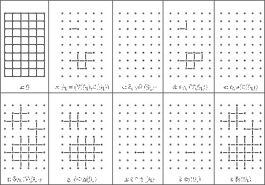
FIGURE 6.1
Dilations and erosions.

Property 4 ([10])

For any $ℰ\left({\mathcal{G}}_1\right)\subseteq ℰ\left(\mathcal{G}\right)$ and $\mathcal{V}\left({\mathcal{G}}_2\right)\subseteq \mathcal{V}\left(\mathcal{G}\right)$:

1.  ${\delta }_{ℰ\mathcal{V}}:ℰ\left(\mathcal{G}\right)\to \mathcal{V}\left(\mathcal{G}\right)$ is such that ${\delta }_{ℰ\mathcal{V}}\left(ℰ\left({\mathcal{G}}_1\right)\right)=\left\{{\upsilon }_i\in \mathcal{V}\left(\mathcal{G}\right)|\exists e_{ij}\in ℰ\left({\mathcal{G}}_1\right)\right\}$;

2.  ${\epsilon }_{\mathcal{V}ℰ}:\mathcal{V}\left(\mathcal{G}\right)\to ℰ\left(\mathcal{G}\right)$ is such that ${\epsilon }_{\mathcal{V}ℰ}\left(\mathcal{V}\left({\mathcal{G}}_2\right)\right)=\left\{e_{ij}\in ℰ\left(\mathcal{G}\right)|{\upsilon }_i\in \mathcal{V}\left({\mathcal{G}}_2\right)and{\upsilon }_j\in \mathcal{V}\left({\mathcal{G}}_2\right)\right\}$;

3.  ${\epsilon }_{ℰ\mathcal{V}}:ℰ\left(\mathcal{G}\right)\to \mathcal{V}\left(\mathcal{G}\right)$ is such that ${\epsilon }_{ℰ\mathcal{V}}\left(ℰ\left({\mathcal{G}}_1\right)\right)=\left\{{\upsilon }_i\in \mathcal{V}\left(\mathcal{G}\right)|\forall e_{ij}\in ℰ\left(\mathcal{G}\right),e_{ij}\in ℰ\left({\mathcal{G}}_1\right)\right\}$;

4.  ${\delta }_{\mathcal{V}ℰ}:\mathcal{V}\left(\mathcal{G}\right)\to ℰ\left(\mathcal{G}\right)$ is such that ${\delta }_{\mathcal{V}ℰ}\left(\mathcal{V}\left({\mathcal{G}}_2\right)\right)=\left\{e_{ij}\in ℰ\left(\mathcal{G}\right)|either{\upsilon }_i\in \mathcal{V}\left({\mathcal{G}}_2\right)or{\upsilon }_j\in \mathcal{V}\left({\mathcal{G}}_2\right)\right\}$.

In other words, ${\delta }_{ℰ\mathcal{V}}\left(ℰ\left({\mathcal{G}}_1\right)\right)$ is the set of all vertices that belong to an edge of $ℰ\left({\mathcal{G}}_1\right),{\epsilon }_{\mathcal{V}ℰ}\left(\mathcal{V}\left({\mathcal{G}}_2\right)\right)$ is the set of all edges whose two extremities are in $\mathcal{V}\left({\mathcal{G}}_2\right),{\epsilon }_{ℰ\mathcal{V}}\left(ℰ\left({\mathcal{G}}_1\right)\right)$ is the set of all vertices which do not belong to any edge of $\overline{ℰ\left({\mathcal{G}}_1\right)}$, and ${\delta }_{\mathcal{V}ℰ}\left(\mathcal{V}\left({\mathcal{G}}_2\right)\right)$ is the set of all edges which have at least one extremity in $\mathcal{V}\left({\mathcal{G}}_2\right)$.

From this characterization, we can recognize the general graph version of some operators introduced by Meyer and Angulo [8] (see also [7]) for the hexagonal grid. By translating supremum and infimum of the graph lattice to the corresponding supremum and infimum of the lattice of weigths, we obtain the weighted version of these operators. The four basic operators of Definition 3 translate to: ${\left({\delta }_{ℰ\mathcal{V}}\left(w\right)\right)}_i=\max \left\{w_{ij}|e_{ij}\in ℰ\right\}$, ${\epsilon }_{ℰ\mathcal{V}}{\left(w\right)}_i=\min \left\{w_{ij}|e_{ij}\in ℰ\right\}$, ${\left({\delta }_{\mathcal{V}ℰ}\left(w\right)\right)}_{ij}=\max \left\{w_i,w_j\right\}$, and ${\left({\epsilon }_{\mathcal{V}ℰ}\left(w\right)\right)}_{ij}=\min \left\{w_i,w_j\right\}$.

Before further analyzing the operators defined above, let us briefly recall some algebraic tools that are fundamental in mathematical morphology [26].

Given two lattices ${ℒ}_1$ and ${ℒ}_2$, an operator $\delta :{ℒ}_1\to {ℒ}_2$ is called a dilation when it preserves the supremum (i.e., $\forall \mathcal{X}\subseteq {ℒ}_1,\delta \left({\vee }_1\mathcal{X}\right)={\vee }_2\left\{\delta \left(x\right)|x\in \mathcal{X}\right\}$, where ∨₁ is the supremum in ${ℒ}_1$ and ∨₂ the supremum in ${ℒ}_2$). Similarly, an operator which preserves the infimum is called an erosion.

Two operators $\epsilon :{ℒ}_1\to {ℒ}_2$ and $\delta :{ℒ}_2\to {ℒ}_1$ form an adjunction (ε, δ) when for any x in ${ℒ}_2$ and any y in ${ℒ}_1$, we have δ(x) ≤₁ y ⇔ x ≤₂ ε(y), where ≤₁ and ≤₂ denote the order relations on, respectively, ${ℒ}_1$ and ${ℒ}_2$. Given two operators ε and δ, if the pair (ε, δ) is an adjunction, then ε is an erosion and δ is a dilation.

Given two complemented lattices ${ℒ}_1$ and ${ℒ}_2$, two operators α and β from ${ℒ}_1$ into ${ℒ}_2$ are dual (with respect to the complement) of each other when, for any $x\in {ℒ}_1$, we have $\beta \left(x\right)=\overline{\alpha \left(\overline{x}\right)}$. If α and β are dual of each other, then β is an erosion whenever α is a dilation.

Property 5 (dilation, erosion, adjunction, duality, [10])

1.  Both $\left({\epsilon }_{\mathcal{V}ℰ},{\delta }_{ℰ\mathcal{V}}\right)$ and $\left({\epsilon }_{ℰ\mathcal{V}},{\delta }_{\mathcal{V}ℰ}\right)$ are adjunctions.

2.  Operators ${\epsilon }_{\mathcal{V}ℰ}$ and ${\delta }_{\mathcal{V}ℰ}$ (respectively ${\epsilon }_{ℰ\mathcal{V}}$ and ${\delta }_{ℰ\mathcal{V}}$) are dual of each other.

3.  Operators ${\delta }_{ℰ\mathcal{V}}$ and ${\delta }_{\mathcal{V}ℰ}$ are dilations.

4.  Operators ${\epsilon }_{ℰ\mathcal{V}}$ and ${\epsilon }_{\mathcal{V}ℰ}$ are erosions.

Let us compose these dilations and erosions to act on $\mathcal{V}\left(\mathbb{G}\right)$ and $ℰ\left(\mathbb{G}\right)$.

Definition 6 (vertex-dilation, vertex-erosion)

We define δ and ε that act on $\mathcal{V}\left(\mathbb{G}\right)$ (i.e., $\mathcal{V}\left(\mathbb{G}\right)\to \mathcal{V}\left(\mathbb{G}\right)$)by $\delta ={\delta }_{ℰ\mathcal{V}}\circ {\delta }_{\mathcal{V}ℰ}$ and $\epsilon ={\epsilon }_{ℰ\mathcal{V}}\circ {\epsilon }_{\mathcal{V}ℰ}$.

As compositions of, respectively, dilations and erosions, δ and ε are, respectively, a dilation and an erosion. Moreover, by composition of adjunctions and dual operators, δ and ε are dual, and (ε, δ) is an adjunction.

In fact, it can be shown that δ and ε correspond exactly to the usual notions of an erosion and of a dilation of a set of vertices in a graph [4, 5]. It means, in particular, that when $\mathcal{V}\left(\mathcal{G}\right)$ is a subset of the grid points ${\mathbb{Z}}^d$ and when the edge set $ℰ\left(\mathcal{G}\right)$ is obtained from a symmetrical structuring element, then the operators defined above are equivalent to the usual binary dilation and erosion by the considered structuring element. For instance, in Figure 6.1, $\mathcal{V}\left(\mathcal{G}\right)$ is a rectangular subset of ${\mathbb{Z}}^2$ and $ℰ\left(\mathcal{G}\right)$ corresponds to the basic “cross” structuring element. It can be verified that the vertex sets in Figure 6.1 (g) and (h), obtained by applying δ and ε to $\mathcal{V}\left({\mathcal{G}}_1\right)$ (Figure 6.1(b), are the dilation and the erosion by a “cross” structuring element of $\mathcal{V}\left({\mathcal{G}}_1\right)$.

We now consider a dual/adjunct pair of dilation and erosion acting on $ℰ\left(\mathbb{G}\right)$.

Definition 7 (edge-dilation, edge-erosion, [10])

We define Δ and $ℰ$ that act on $ℰ\left(\mathbb{G}\right)$ by $\Delta ={\delta }_{\mathcal{V}ℰ}\circ {\delta }_{ℰ\mathcal{V}}$ and $ℰ={\epsilon }_{\mathcal{V}ℰ}\circ {\epsilon }_{ℰ\mathcal{V}}$.

Definition 8 ([10])

We define the operators and by, respectively, $\left(\delta \left(\mathcal{V}\left({\mathcal{G}}_1\right)\right),\Delta \left(ℰ\left({\mathcal{G}}_1\right)\right)\right)$ and $\left(\epsilon \left(\mathcal{V}\left({\mathcal{G}}_1\right)\right),ℰ\left(ℰ\left({\mathcal{G}}_1\right)\right)\right)$, for any ${\mathcal{G}}_1\in \mathbb{G}$.

For instance, Figures 6.1(f) and 6.1(g) present the results obtained by applying the operator and the operator to the subgraph ${\mathcal{G}}_1$ (Figure 6.1(b)) of $\mathcal{G}$ (Figure 6.1(a)).

Theorem 9 (graph-dilation, graph-erosion,[10])

The operators and are respectively a dilation and an erosion acting on the lattice $\left(\mathbb{G},⊑\right)$. Furthermore, is an adjunction.

Note that since lattice $\mathbb{G}$ is sup-generated by set $\mathcal{S}$, it suffices to know the dilation of the graphs in $\mathcal{S}$ for characterizing the dilation of the graphs in $\mathbb{G}$.

Compared to classical morphological operators on sets, the dilations and erosions introduced in this section furthermore convey some connectivity properties different than the ones which can be deduced from classical dilations and erosions. Observe, for instance, in Figure 6.1(g), that some 4-adjacent vertices of $\delta \left(\mathcal{V}\left({\mathcal{G}}_1\right)\right)$ are not linked by an edge in the graph . These properties can be useful in further processing involving for instance connected operators [27, 28, 29, 30].

Thanks to the operators presented in Definition 3, other intersecting adjunctions (hence dilations/erosions) can be defined on $\mathbb{G}$:

1.  (α₁, β₁) such that $\forall {\mathcal{G}}_1\in \mathbb{G},{\alpha }_1\left({\mathcal{G}}_1\right)=\left(\mathcal{V}\left(\mathcal{G}\right),ℰ\left({\mathcal{G}}_1\right)\right)$ and ${\beta }_1\left({\mathcal{G}}_1\right)=\left({\delta }_{ℰ\mathcal{V}}\left(ℰ\left({\mathcal{G}}_1\right)\right),ℰ\left({\mathcal{G}}_1\right)\right)$;

2.  (α₂, β₂) such that $\forall {\mathcal{G}}_1\in \mathbb{G},{\alpha }_2\left({\mathcal{G}}_1\right)=\left(\mathcal{V}\left({\mathcal{G}}_1\right),{\epsilon }_{\mathcal{V}ℰ}\left(\mathcal{V}\left({\mathcal{G}}_1\right)\right)\right)$ and ${\beta }_2\left({\mathcal{G}}_1\right)=\left(\mathcal{V}\left({\mathcal{G}}_1\right),\cancel{0}\right)$;

3.  (α₃, β₃) such that $\forall {\mathcal{G}}_1\in \mathbb{G},{\alpha }_3\left({\mathcal{G}}_1\right)=\left({\epsilon }_{ℰ\mathcal{V}}\left(ℰ\left({\mathcal{G}}_1\right)\right),{\epsilon }_{\mathcal{V}ℰ}\circ {\epsilon }_{ℰ\mathcal{V}}\left(ℰ\left({\mathcal{G}}_1\right)\right)\right)$ and ${\beta }_3\left({\mathcal{G}}_1\right)=\left({\delta }_{ℰ\mathcal{V}}\circ {\delta }_{\mathcal{V}ℰ}\left(\mathcal{V}\left({\mathcal{G}}_1\right)\right),{\delta }_{\mathcal{V}ℰ}\left(\mathcal{V}\left({\mathcal{G}}_1\right)\right)\right)$.

The adjunction (α₃, β₃) is illustrated in Figures 6.1(i) and 6.1(j). Note also that, using usual graph terminologies, β₁ (respectively α₂) can be defined as the operator which associates to a graph the graph induced by its edge set (respectively, vertex set).

A more general version of those operators can be obtained in the framework of complexes [12], allowing us to deal for example with meshes. There also exist other recent graph-based approaches to morphology, for example based on hypergraphs [11] or on discrete differential equations [9].

6.4    Filters

In mathematical morphology, a filter is an operator α acting on a lattice $ℒ$ that is increasing (i.e., $\forall x,y\in ℒ,\alpha \left(x\right)\le \alpha \left(y\right)$ whenever x ≤ y) and idempotent (i.e., $\forall x\in ℒ,\alpha \left(\alpha \left(x\right)\right)=\alpha \left(x\right)$). A filter α on $ℒ$ that is extensive (i.e., $\forall x\in ℒ,x\le \alpha \left(x\right)$) is called a closing on $ℒ$, whereas a filter α on $ℒ$ that is anti-extensive (i.e., $\forall x\in ℒ$, α(x) ≤ x) is called an opening on $ℒ$. It is known that composing the two operators of an adjunction yields an opening or a closing, depending on the order in which the operators are composed [26]. In this section, the operators of Section 6.3 are composed to obtain filters on $\mathcal{V}\left(\mathbb{G}\right),ℰ\left(\mathbb{G}\right)$ and $\mathbb{G}$.

Definition 10 (opening, closing, [10])

1.  We define γ₁ and ϕ₁, which act on $\mathcal{V}\left(\mathbb{G}\right)$, by γ₁ = δ ∘ ε and ϕ₁ = ε ∘ δ.

2.  We define Γ₁ and Φ₁, which act on $ℰ\left(\mathbb{G}\right)$, by ${\Gamma }_1=\Delta \circ ℰ$ and ${\Phi }_1=ℰ\circ \Delta$.

3.  We define the operators and by, respectively, , and for any ${\mathcal{G}}_1\in \mathbb{G}$.

Figures 6.2(b) and 6.2(f) present the result of and for, respectively, the subgraph of Figure 6.2(a) and the one of Figure 6.2(e).

The opening γ₁ and the closing ϕ₁ correspond to the classical opening and closing on the vertices. The closing Γ₁ and the opening Φ₁ are the corresponding edge-version of these operators. By combination, we obtain and .

In fact, by composing ${\delta }_{ℰ\mathcal{V}}$ with ${\epsilon }_{\mathcal{V}ℰ}$ and ${\delta }_{ℰ\mathcal{V}}$ with ${\epsilon }_{\mathcal{V}ℰ}$, we obtain smaller filters.

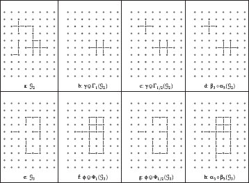
FIGURE 6.2
Openings and closings ($\mathcal{G}$ is induced by the 4-adjacency relation).

Definition 11 (half-opening, half-closing, [10])

1.  We define γ_1/2 and ϕ_1/2, that act on $\mathcal{V}\left(\mathbb{G}\right)$, by ${\gamma }_{1/2}={\delta }_{ℰ\mathcal{V}}\circ {ϵ}_{\mathcal{V}ℰ}$ and ${\varphi }_{1/2}={\epsilon }_{ℰ\mathcal{V}}\circ {\delta }_{\mathcal{V}ℰ}$.

2.  We define Γ_1/2 and Φ_1/2, that act on $ℰ\left(\mathbb{G}\right)$ by ${\Gamma }_{1/2}={\delta }_{\mathcal{V}ℰ}\circ {\epsilon }_{ℰ\mathcal{V}}$ and ${\Phi }_{1/2}={\epsilon }_{\mathcal{V}ℰ}\circ {\delta }_{ℰ\mathcal{V}}$.

3.  We define the operators and by, respectively, and , for any ${\mathcal{G}}_1\in \mathbb{G}$.

Thanks to Property 4, the operators defined above can be locally characterized. Let $\mathcal{V}\left({\mathcal{G}}_1\right)\subseteq \mathcal{V}\left(\mathcal{G}\right)$ and $ℰ\left({\mathcal{G}}_2\right)\subseteq ℰ\left(\mathcal{G}\right)$, we have:

$\begin{array}{lll}{\gamma }_{1/2}\left(\mathcal{V}\left({\mathcal{G}}_1\right)\right)\hfill & =\hfill & \left\{{\upsilon }_i\in \mathcal{V}\left({\mathcal{G}}_1\right)|\exists e_{ij}\in ℰ\left(\mathcal{G}\right)\text{with}{\upsilon }_j\in \mathcal{V}\left({\mathcal{G}}_1\right)\right\}\hfill \\ \hfill & =\hfill & \mathcal{V}\left({\mathcal{G}}_1\right)\left\{{\upsilon }_i\in \mathcal{V}\left({\mathcal{G}}_1\right)|\forall e_{ij}\in ℰ\left(\mathcal{G}\right),{\upsilon }_j\notin \mathcal{V}\left({\mathcal{G}}_1\right)\right\}\hfill \\ {\Gamma }_{1/2}\left(ℰ\left({\mathcal{G}}_2\right)\right)\hfill & =\hfill & \left\{e_{ij}\in ℰ\left(\mathcal{G}\right)|\left\{e_{ik}\in ℰ\left(\mathcal{G}\right)\right\}\subseteq ℰ\left({\mathcal{G}}_2\right)\right\}\hfill \\ \hfill & =\hfill & ℰ\left(G_2\right)\left\{e\in ℰ\left(Y\right)|\forall {\upsilon }_i\in e,\exists e_{ij}\in ℰ\left(\mathcal{G}\right)\text{with}{e}_{ij}\notin ℰ\left({\mathcal{G}}_2\right)\right\}\hfill \\ {\varphi }_{1/2}\left(\mathcal{V}\left({\mathcal{G}}_1\right)\right)\hfill & =\hfill & \left\{{\upsilon }_i\in \mathcal{V}\left(\mathcal{G}\right)|\text{either}{\upsilon }_i\in \mathcal{V}\left({\mathcal{G}}_1\right)\text{or}\forall e_{ij}\in ℰ\left(\mathcal{G}\right),{\upsilon }_j\in \mathcal{V}\left({\mathcal{G}}_1\right)\right\}\hfill \\ \hfill & =\hfill & \mathcal{V}\left({\mathcal{G}}_1\right)\cup \left\{{\upsilon }_i\in \overline{\mathcal{V}\left({\mathcal{G}}_1\right)}|\forall e_{ij}\in ℰ\left(\mathcal{G}\right),{\upsilon }_j\in \mathcal{V}\left({\mathcal{G}}_1\right)\right\}\hfill \\ {\Phi }_{1/2}\left(ℰ\left({\mathcal{G}}_2\right)\right)\hfill & =\hfill & \left\{e_{ij}\in ℰ\left(\mathcal{G}\right)|\exists e_{ik}\in ℰ\left({\mathcal{G}}_2\right)\text{and}\exists e_{jl}\in ℰ\left({\mathcal{G}}_2\right)\right\}\hfill \\ \hfill & =\hfill & Y\cup \left\{e_{ij}\in \overline{ℰ\left({\mathcal{G}}_2\right)}|{\upsilon }_i\in {\delta }_{ℰ\mathcal{V}}\left(ℰ\left({\mathcal{G}}_2\right)\right)\text{and}{\upsilon }_j\in {\delta }_{ℰ\mathcal{V}}\left(ℰ\left({\mathcal{G}}_2\right)\right)\right\}.\hfill \end{array}$

Informally speaking, γ_1/2 removes from ${\mathcal{G}}_1$ its isolated vertices, whereas Γ_1/2 removes from ${\mathcal{G}}_2$ the edges that do not contain a vertex completely covered by edges in ${\mathcal{G}}_2$. It may be seen furthermore that γ_1/2 (respectively, Γ_1/2) is the dual of ϕ_1/2 (respectively, Φ_1/2). Thus, ϕ_1/2 adds to ${\mathcal{G}}_1$ the vertices of $\overline{\mathcal{V}\left({\mathcal{G}}_1\right)}$ completely surrounded by elements of ${\mathcal{G}}_1$ whereas Φ_1/2 adds to ${\mathcal{G}}_2$ the edges of $\overline{ℰ\left({\mathcal{G}}_2\right)}$ whose two extremities belong to at least one edge in ${\mathcal{G}}_2$ (see, for instance, Figure 6.2).

The family $\mathbb{G}$ is closed under the operators presented in Definition 10.3 since they are obtained by composition of operators also satisfying this property. Furthermore, it can be deduced from the local characterization of the operators γ_1/2, Γ_1/2, ϕ_1/2 and Φ_1/2 that the family $\mathbb{G}$ is also closed under the operators of Definition 11.3. Hence, thanks to the properties of adjunctions recalled in the introduction of this section, the following theorem can be established.

Theorem 12 (graph-openings, graph-closings,[10])

1.  The operators γ_1/2 and γ₁ (respectively, Γ_1/2 and Γ₁) are openings on $\mathcal{V}\left(\mathbb{G}\right)$ (respectively, $ℰ\left(\mathbb{G}\right)$) and ϕ_1/2, and Φ₁ (respectively, Φ_1/2 and ϕ₁) are closings on $\mathcal{V}\left(\mathbb{G}\right)$ (respectively, $ℰ\left(\mathbb{G}\right)$).

2.  The family $\mathbb{G}$ is closed under , , , and .

3.  The operators and are openings on $\mathbb{G}$ and , and are closings on $\mathbb{G}$.

Composing the operators of the adjunctions (α_i, β_i), defined at the end of Section 6.3, also yields remarkable openings and closings. Indeed, it can be easily seen that: α₁ ∘ β₁ = α₁, α₂ ∘ β₂ = α₂, β₁ ∘ α₁ = β₁, and β₂ ∘ α₂ = β₂. Thus, α₁ and α₂ are both a closing and an erosion, and β₁ and β₂ are both a dilation and an opening. This means, in particular, that α₁ and α₂ are idempotent extensive erosions and that β₁ and β₂ are idempotent anti-extensive dilations. The opening and the closing resulting from the adjunction (α₃, β₃) are illustrated in Figures 6.2d and 6.2h.

The weighted versions of those various operators also have an interpretation related to classical notions of graph theory. Consider, for example, the weighted version of the opening ${\Gamma }_{1/2}={\delta }_{\mathcal{V}ℰ}{\epsilon }_{ℰ\mathcal{V}}$. The dilation ${\delta }_{\mathcal{V}ℰ}$ assigns to each edge the highest weight of its adjacent vertices; but each adjacent vertice has been assigned by ${\epsilon }_{ℰ\mathcal{V}}$ the weight of its lowest edge. So if w_ij is left unchanged by Γ_1/2, it means that the edge e_ij is (one of) the lowest edges of υ_i or of υ_j, say υ_i. Its weight is higher or equal to the weight of the lowest edge of υ_j. Thus, using some well-known properties of minimum spanning trees (see Section 6.6.3 for a precise definition of a minimum spanning tree), it can be shown that the graph induced by the set of edges that are left invariant by Γ_1/2 is the union of all mininimum spanning trees of this graph, closely related to the Gabriel graph [31].

It is possible to associate with any lattice $ℒ$, the lattice of all increasing operators on $ℒ$. In this context, two filters, φ₁ and φ₂, on the lattice $ℒ$ are said ordered if, for any ∈ $ℒ$, φ₁(x) ≤ φ₂(x) or if, for any $x\in ℒ$, φ₂(x) ≤ φ₁(x). A usual way to build a hierarchy of filters (i.e., an ordered family of filters) from an adjunct pair (α, β) of erosion and dilation consists of building the dilations and erosions obtained by iterating several times α and β. In general, composing these iterated versions of α and β leads to hierarchies of filters when the number of iterations increases. By combining and iterating the operators that we have defined in this section, we obtain [10] hierarchies of filters in the lattice $\mathbb{G}$ that perform better than the classical ones, in the sense that they are able to remove more noise (see Figure 6.3.)

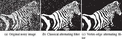
FIGURE 6.3
Illustration of classical versus vertex-edge alternating filter (see [10]).

6.5    Connected Operators and Filtering with the Component Tree

Gray-level connected operators [27] act by merging neighboring “flat” zones. They cannot create new contours and, as a result, they cannot introduce in the output image a structure that is not present in the input image. Furthermore, they cannot modify the position of existing boundaries between regions, and therefore have very good contour preservation properties.

To create “flat” zones, a simple operation on a weighted graph is thresholding, that produces a level set. For $\lambda \in {ℝ}^{+}$, the level-sets of an edge-weighted graph are denoted $w_{ℰ}^{<}\left[\lambda \right]=\left\{e_{ij}\in ℰ|w_{ij}\le \lambda \right\}$. We define ${\mathcal{C}}_{ℰ}^{<}$ as the set composed of all the pairs [λ, C}, where $\lambda \in {ℝ}^{+}$ and C is a (connected) component of the graph $w_{ℰ}^{<}\left[\lambda \right]$.

We note that one can reconstruct w from ${\mathcal{C}}_{ℰ}^{<}$; more precisely, we have:

$w_{ij}=\min \left\{\lambda |\left[\lambda ,C\right]\in {\mathcal{C}}_{ℰ}^{<},e_{ij}\in ℰ\left(C\right)\right\}$

(6.1)

One can remark that two elements of ${\mathcal{C}}_{ℰ}^{<}$ are either disjoint or nested, thus it is easy to order the elements of ${\mathcal{C}}_{ℰ}^{<}$ in a tree. This tree is called the (min) component tree, and there exists fast algorithms to compute it [32, 33].

Using ${\mathcal{C}}_{ℰ}^{<}$ allows us to deal with specific components of w. For example, a minimum of w is a component C such that there exists λ with $\left[\lambda ,C\right]\in {\mathcal{C}}_{ℰ}^{<}$, and it does not exist $\left[{\lambda }_1,C_1\right]\in {\mathcal{C}}_{ℰ}^{<}$ with C₁ ⊏ C and C₁ ≠ C. Observe that a minimum of w is a graph. The set of all minima of w is denoted $ℳ$. Similarly, we can define ${\mathcal{C}}_{ℰ}^{>}$ allowing us to deal with maxima of edge-weighted graphs ${\mathcal{C}}_{\mathcal{V}}^{<}$ and ${\mathcal{C}}_{\mathcal{V}}^{>}$, allowing us to deal with node-weighted graphs, and ${\mathcal{C}}_{\mathcal{V}ℰ}^{<}$, and ${\mathcal{C}}_{\mathcal{V}ℰ}^{<}$ allowing us to deal with node- and edge-weighted graphs.

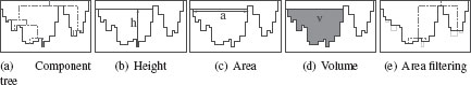
FIGURE 6.4
Illustration of, respectively, a component tree (dashed lines), the height, the area, and the volume of a component and an area filtering.

We mention that other trees are possible, for example, the binary partition tree [34], the tree of level lines, also known as the inclusion tree or the tree of shapes [35], etc. The interest of the tree of shapes is that it allows us to interact both with maxima and minima, in a self-dual manner. See [36] for a survey of the usage of those trees in image processing. Here, we illustrate the usage of the component tree for filtering.

Given Equation (6.1), filtering a graph can be seen as equivalent to removing some components of (say) ${\mathcal{C}}_{ℰ}^{<}$. Such a filtering is called flooding. One way to make this idea practicable is to design an attribute that tells us if a given component should be kept or not. Among the numerous attributes that can be computed, three are natural: the height, the area, and the volume (Figure 6.4). Let $\left[\lambda ,C\right]\in {\mathcal{C}}_{ℰ}^{<}$. We define

$\begin{array}{ccc}\text{height}\left(\left[\lambda ,C\right]\right)& =& \max \left\{\lambda -w_{ij}|e_{ij}\in ℰ\left(C\right)\right\}\end{array}$

(6.2)

$\begin{array}{ccc}\text{area}\left(\left[\lambda ,C\right]\right)& =& \left|\mathcal{V}\left(C\right)\right|\end{array}$

(6.3)

$\begin{array}{ccc}\text{volume}\left(\left[\lambda ,C\right]\right)& =& {\displaystyle \sum _{e_{ij}\in ℰ\left(C\right)}\left(\lambda -w_{ij}\right)}\end{array}$

(6.4)

For example, removing all the components whose area is lower than a threshold is a closing of w (Figure 6.4.e). Note that a filtering with either the height or the volume is not a closing, as such a filtering is not idempotent.

Figure 6.5 illustrates this kind of filtering. Figure 6.5.a is an image of a cell in which we want to extract the ten bright lobes. If we consider that the brighter a pixel is, the higher its weight, then the tree we want to process is ${\mathcal{C}}_{\mathcal{V}}^{>}$. Figure 6.5.b shows that Figure 6.5(a) contains numerous maxima. Figure 6.5(c) is the filtered image obtained by a volume-based filtering, and Figure 6.5(d) shows the maxima of this filtered image.

As the components of the level sets can be ordered into a tree, they form a hierarchy of components. In the context of classification [37], hierarchies are widely studied, and the morphological framework can shed some light on the tools that are developed in that community. For example, let us look at the application Ψ that associates to any set of edge-weights w the map Ψ(w) such that for any edge $e_{ij}\in ℰ$, $\Psi \left(w\right)\left(e_{ij}\right)=\min \left\{\lambda |\left[\lambda ,C\right]\in {\mathcal{C}}_{ℰ}^{<},{\upsilon }_i\in \mathcal{V}\left(C\right),{\upsilon }_j\in \mathcal{V}\left(C\right)\right\}$. Intuitively, and using a geographical metaphore, Ψ(w)(e_ij) is the lowest altitude to which one has to climb to go from υ_i to υ_j. It is straightforward to see that Ψ(w) ≤ w, that Ψ(Ψ(w)) = Ψ(w) and that if w′ ≤ w, Ψ(w′) ≤ Ψ(w). Thus, Ψ is an opening [38]. We remark that the subset of strictly positive maps that are defined on the complete graph $\left(\mathcal{V},\mathcal{V}\times \mathcal{V}\right)$ and that are open with respect to Ψ is the set of ultrametric distances on $\mathcal{V}$. The mapping Ψ is known under several names, including “subdominant ultrametric” and “ultrametric opening”. It is well known that Ψ is associated to the simplest method for hierarchical classification called single linkage clustering [39, 40], closely related to Kruskal’s algorithm [41] for computing a minimum spanning tree.

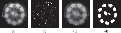
FIGURE 6.5
(a) Original image. (b) Maxima of image (a), in white. (c) Filtered image. (d) Maxima of image (c), which corresponds to the ten most significant lobes of the image (a).

Before concluding the section, let us mention another flooding that has been used as a preprocessing step for watershed segmentation with markers. It is called geodesic reconstruction from the markers [42, 43], where the markers is a subgraph. It consists in removing all the components of ${\mathcal{C}}_{ℰ}^{<}$ that are not marked (i.e., that do not contain a vertice of the markers) and is given as a function w_R such that, for every edge e, we set w_R(e) to be equal to the level λ of the lowest component of w containing e and at least one vertice of the markers. Observe that any component of w_R indeed contains at least one vertice of the markers. Given some markers, the geodesic reconstruction is a closing. Such a closing is also useful as an efficient preprocessing for a fast power-watershed optimization algorithm (see [15] and Section 6.8).

6.6    Watershed Cuts

There exist many possible ways for defining a watershed [24, 44, 45, 46, 13, 47]. Intuitively, the watershed of a function (seen as a topographical surface) is composed of the locations from which a drop of water could flow towards different minima. The framework of edge-weighted graph allows the formalization of this principle and the proof of several remarkable properties [13] that we review in the sequel of the section. We first show that watershed cuts can be equivalently defined by their “catchment basins” (through a steepest descent property) or by the “dividing lines” separating these catchment basins (through the drop of water principle). As far as we know, in discrete frameworks, a similar property does not hold. The second property establishes the optimality of watershed-cuts: there is an equivalence between the watershed-cuts and the separations induced by a minimum spanning forest relative to the minima.

6.6.1    The Drop of Water Principle

Definition 13 (from Definition 12 in [46])

Let ${\mathcal{G}}_1$ and ${\mathcal{G}}_2$ be two non-empty subgraphs of $\mathcal{G}$. We say that ${\mathcal{G}}_2$ is an extension of ${\mathcal{G}}_1$ (in $\mathcal{G}$) if ${\mathcal{G}}_1⊑{\mathcal{G}}_2$ and if any component of ${\mathcal{G}}_2$ contains exactly one component of ${\mathcal{G}}_1$.

The notion of extension is very general. Many segmentation algorithms iteratively extend some seed components in a graph; they produce an extension of the seeds. Most of them terminate once they have reached an extension that cover all the vertices of the graph. The separation thus produced is called a graph cut. Let $\mathcal{S}\subseteq ℰ$. We denote by $\mathcal{S}$ the complementary set of $\mathcal{S}$ in $ℰ$, i.e., $\overline{\mathcal{S}}=ℰ\mathcal{S}$. Recall that the graph induced by $\mathcal{S}$, given by the dilation β₁, is the graph whose edge set is $\mathcal{S}$ and whose vertex set is made of all points that belong to an edge in $\mathcal{S}$, i.e., $\left(\left\{\upsilon \in \mathcal{V}|\exists e\in \mathcal{S},\upsilon \in e\right\},\mathcal{S}\right)$. In the following, the graph induced by $\mathcal{S}$ is also denoted by $\mathcal{S}$.

Definition 14

Let ${\mathcal{G}}_1⊑\mathcal{G}$ and $\mathcal{S}\subseteq ℰ$. We say that $\mathcal{S}$ is a (graph) cut for ${\mathcal{G}}_1$ if $\overline{\mathcal{S}}$ is an extension of ${\mathcal{G}}_1$ and if $\mathcal{S}$ is minimal for this property, i.e., if $\mathcal{T}\subseteq \mathcal{S}$ and $\overline{\mathcal{T}}$ is an extension of ${\mathcal{G}}_1$, then we have $\mathcal{T}=\mathcal{S}$.

We introduce the watershed cuts of an edge-weighted graph. To this end, we formalize the drop of water principle. Intuitively, the catchment basins constitute an extension of the minima, and they are separated by “lines” from which a drop of water can flow down towards distinct minima.

Let π = (υ₀, ⋯, υ_n) be a path. The path π is descending if, for any i ∈ [1, l – 1], w(υ_i−1, υ_i) ≥ w(υ_i, υ_i+1).

Definition 15 (drop of water principle, [13])

Let $\mathcal{S}\subseteq ℰ$. We say that $\mathcal{S}$ is a watershed cut (or simply a watershed) if $\overline{\mathcal{S}}$ is an extension of $ℳ$ and if for any $e_{ij}=\left[{\upsilon }_i,{\upsilon }_j\right]\in \mathcal{S}$, there exist ${\pi }_1=\left({\upsilon }_0^1={\upsilon }_i,\cdots ,{\upsilon }_n^1\right)$ and ${\pi }_2=\left({\upsilon }_0^2={\upsilon }_j,\cdots ,{\upsilon }_m^2\right)$, which are two descending paths in $\overline{\mathcal{S}}$, such that ${\upsilon }_n^1$ and ${\upsilon }_m^2$ are vertices of two distinct minima of w; $w_{ij}\ge w\left(\left\{{\upsilon }_0^1,{\upsilon }_1^1\right\}\right)$ (respectively, $w_{ij}\ge w\left(\left\{{\upsilon }_0^2,{\upsilon }_1^2\right\}\right)$), whenever π₁ (respectively, π₂) is not trivial.

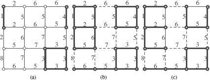
FIGURE 6.6
An edge-weighted graph $\mathcal{G}$ The edges and vertices drawn in bold are (a), the minima of w; (b), an extension of $ℳ$; (c), an MSF rooted in $ℳ$. In (b), the set of dashed edges is a watershed cut of w.

We illustrate the previous definition on the edge-weighted graph depicted in Figure 6.6. The weights w contain three minima (in bold in Figure6.6(a)). Let us denote by $\mathcal{S}$ the set of dashed edges depicted in Figure 6.6(b) and by e = {υ₁, υ₂} the only edge whose altitude is 8. It may be seen that $\overline{\mathcal{S}}$ (in bold Figure 6.6(b)) is an extension of $ℳ$. We also remark that there exists π₁ (respectively π₂) a descending path in $\overline{\mathcal{S}}$ from υ₁ (respectively υ₂) to the minimum at altitude 1 (respectively, 3). The altitude of the first edge of π₁ (respectively, π₂) is lower than the altitude of e. It can be verified that the previous properties hold true for any edge in $\mathcal{S}$. Thus, $\mathcal{S}$ is a watershed of F.

6.6.2    Catchment Basins by a Steepest Descent Property

A popular alternative to Definition 15 consists of defining a watershed exclusively by its catchment basins and the paths of steepest descent of w [48, 44, 49, 45], and does not involve any property of the divide. The following theorem (17) establishes the consistency of watershed cuts in edge-weighted graphs: they can be equivalently defined by a steepest descent property on the catchment basins (regions) or by the drop of water principle on the cut (border) which separate them. As far as we know, there is no definition of watershed in vertex-weighted graphs that verifies a similar property. This theorem thus emphasizes that the framework of edge-weighted graphs is adapted for the study of discrete watersheds.

Let π = (υ₀, ⋯, υ_l) be a path in $\mathcal{G}$. The path π is a path of steepest descent (for w) if, for any i ∈ [1, l], $w\left({\upsilon }_{i-1},{\upsilon }_i\right)={\left({\epsilon }_{ℰ\mathcal{V}}w\right)}_{i-1}=\min \left\{w_{ij}|\forall j\text{such}\text{that}{e}_{ij}\in ℰ\right\}$.

Definition 16 ([13])

Let $\mathcal{S}\subseteq ℰ$ be a cut for $ℳ$. We say that $\mathcal{S}$ is a basin cut (of w) if, from each point of $\mathcal{V}$ to $ℳ$, there exists, in the graph induced by $\overline{\mathcal{S}}$, a path of steepest descent for w. If $\mathcal{S}$ is a basin cut of w, any component of $\overline{\mathcal{S}}$ is called a catchment basin (of w, for $\mathcal{S}$).

Theorem 17 (consistency, [13])

Let $\mathcal{S}\subseteq ℰ$ be a cut for $ℳ$. The set $\mathcal{S}$ is a watershed if and only if $\mathcal{S}$ is a basin cut of w.

6.6.3    Minimum Spanning Forests

We establish the optimality of watersheds. To this end, we introduce the notion of minimum spanning forests rooted in some subgraphs of $\mathcal{G}$. Each of these forests induces a unique graph cut. The main result of this study (Th. 19) states that a graph cut is induced by a minimum spanning rooted in the minima of a function if and only if it is a watershed of this function.

Definition 18 (rooted MSF, [14])

Let ${\mathcal{G}}_1$ and ${\mathcal{G}}_2$ be two nonempty subgraphs of $\mathcal{G}$. We say that ${\mathcal{G}}_2$ is rooted in ${\mathcal{G}}_1$ if $\mathcal{V}\left({\mathcal{G}}_1\right)\subseteq \mathcal{V}\left({\mathcal{G}}_2\right)$ and if the vertex set of any component of ${\mathcal{G}}_2$ contains the vertex set of exactly one component of ${\mathcal{G}}_1$. Recall that the weight of ${\mathcal{G}}_1$ is the sum of its weight, i.e., ${\displaystyle {\sum }_{e_{ij}\in ℰ\left(G_1\right)}{w}_{ij}}$

We say that ${\mathcal{G}}_2$ is a minimum spanning forest (MSF) rooted in ${\mathcal{G}}_1$ if (1) ${\mathcal{G}}_2$ is spanning for $\mathcal{V}$, (2) ${\mathcal{G}}_2$ is rooted in ${\mathcal{G}}_1$, and (3) the weight of ${\mathcal{G}}_2$ is less than or equal to the weight of any graph ${\mathcal{G}}_3$ satisfying (1) and (2) (i.e., ${\mathcal{G}}_3$ is both spanning for $\mathcal{V}$ and rooted in ${\mathcal{G}}_1$). The set of all minimum spanning forests rooted in ${\mathcal{G}}_1$ is denoted by MSF(G₁).

The above definition of rooted MSFs allows the usual notions of graph theory based on trees and forests to be recovered. In particular, if υ is a vertex of V, it can be seen that any element in MSF({υ}, $\cancel{0}$) is a minimum spanning tree of (G, w), and that, conversely, any minimum spanning tree of (G, w) belongs to MSF({υ}, $\cancel{0}$).

Let us consider the edge-weighted graph $\mathcal{G}$ and the subgraph $ℳ$ (in bold) of Figure 6.6(a). It can be verified that the graph ${\mathcal{G}}_1$ (in bold in Figure 6.6(c)) is an MSF rooted in $ℳ$.

We now have the mathematical tools to present the main result of this section (Th. 19), which establishes the optimality of watersheds.

Let ${\mathcal{G}}_1$ be a subgraph of $\mathcal{G}$ and let ${\mathcal{G}}_2$ be a spanning forest rooted in ${\mathcal{G}}_1$. There exists a unique cut for ${\mathcal{G}}_2$, and this cut is also a cut for ${\mathcal{G}}_1$. We say that this unique cut is the cut induced by ${\mathcal{G}}_2$.

Theorem 19 (optimality, [13])

Let $\mathcal{S}\subseteq ℰ$. The set $\mathcal{S}$ is a cut induced by a MSF rooted in $ℳ$ if and only if $\mathcal{S}$ is a watershed cut.

6.6.4    Illustrations to Segmentation

In this subsection, we illustrate the versatility of the proposed framework to perform segmentation on different kinds of geometric objects. Firstly, we show how to segment triangulated surfaces by watershed cuts, and, secondly, we apply the watershed cuts to the segmentation of diffusion tensors images, which are medical images associating a tensor to each voxel.

3D shape acquisition and digitizing have received more and more attention for a decade, leading to an increasing amount of 3D surface-models (or meshes) such as the one in Figure 6.7(d). In a recent work [50], a new search engine has been proposed for indexing and retrieving objects of interests in a database of meshes (EROS 3D) provided by the French Museum Center for Research. One key idea of this search engine is to use region descriptors rather than global shape descriptors. In order to produce such descriptors, it is then essential to obtain meaningful mesh segmentations.

Informally, a mesh M in the 3D Euclidean space is a set of triangles, sides of triangles, and points such that each side is included in exactly two triangles (see Figure 6.7(a)). In order to perform a watershed cut on such a mesh, we build a graph $\mathcal{G}=\left(\mathcal{V},ℰ\right)$ whose vertex set $\mathcal{V}$ is the set of all triangles in M and whose edge set $ℰ$ is composed by the pairs e_ij = {υ_i, υ_j} such that υ_i and υ_j are two triangles of M that share a common side (see Figure 6.7(a)). The graph $\mathcal{G}$ is known under the term 2-dual of the surface mesh [51].

To obtain a segmentation of the mesh M thanks to a watershed cut, we need to weight the edges of $\mathcal{G}$ (or equivalently the sides of M) by a map whose values are high around the boundaries of the regions that we want to separate. We have found that the interesting contours on the EROS 3D meshes are mostly located on concave zones. Therefore, we weight the edges of $\mathcal{G}$ by a weighting w, which behaves like the inverse of the mean curvature of the surface (see [50] for more details). Then, we can compute a watershed cut (in bold in Figure 6.7(b)) which leads to a natural and accurate mesh segmentation in the sense that the “borders” of the regions are made of sides of triangles (in bold in Figure 6.7c) of high curvature.

The direct application of this method on the mesh shown Figure 6.7(d) leads to a strong over-segmentation (Figure 6.7(e)) due to the huge number of local minima. By using the methodology introduced in Section 6.5 to remove from w all the minima which have a depth lower than a predefined threshold (here, 50) A watershed cut of the filtered w is depicted in Figure 6.7(f).

In the medical context, Diffusion Tensor Images (DTIs) [52] provide a unique insight into oriented structures within tissues. A DTI T maps the set of voxels $\mathcal{V}\subseteq {\mathbb{Z}}^3$ (i.e., $\mathcal{V}$ is a cuboid of ${\mathbb{Z}}^3$) into the set of 3 × 3 tensors (i.e., 3 × 3 symmetric positive definite matrices). The value T(υ) of a DTI T at a voxel $\upsilon \in \mathcal{V}$ describes the diffusion of water molecules at υ. For instance, the first eigenvector of T(υ) (i.e., the one whose associated eigenvalue is maximal) provides the principal direction of water molecules diffusion at point x and its associated eigenvalue gives the magnitude of the diffusion along this direction. Since water molecules highly diffuse along fiber tracts and since the white matter of the brain is mainly composed of fiber tracts, DTIs are particularly adapted to the study of brain architecture. Figure 6.8a shows a representation of a cross-section of a brain DTI where the tensors are represented by ellipsoids. Indeed, the data of a tensor is equivalent to the one of an ellipsoid. In the brain, the corpus callosum is an important structure made of fiber tracts connecting homologous areas of each hemisphere. In order to track the fibers that pass through the corpus callosum, it is necessary to segment it first. The next paragraph briefly reviews how to reach this goal, thanks to watershed cuts [47].

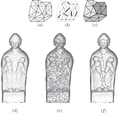
FIGURE 6.7
Surface segmentation by watershed cut. (a) A mesh in black and its associated graph in gray. (b) A cut on this graph (in bold); and (c), the corresponding segmentation of the mesh. (d) Rendering of the mesh of a sculpture. (e) A watershed (in red) of a map F which behaves like the inverse of the mean curvature and, in (f), a watershed of a filtered version of F. The mesh shown in (d) is provided by the French Museum Center for Research.

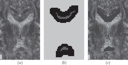
FIGURE 6.8
Diffusion tensor images segmentation. (a) A close-up on a cross-section of a 3D brain DTI. (b) Image representation of the markers (same cross-section as (a)), obtained from a statistical atlas, for the corpus callosum (dark gray) and for its background (light gray) (c) Segmentation of the corpus callosum by an MSF-cut for the markers. The tensors belonging to the component of the MSF that extends the marker labelled “corpus callosum” are removed from the initial DTI thus, the corresponding voxels appear black.

We consider the graph $\mathcal{G}=\left(\mathcal{V},ℰ\right)$ induced by the 6-adjacency and defined by $e_{ij}\in ℰ$ iff ${\upsilon }_i\in \mathcal{V},{\upsilon }_j\in \mathcal{V}$ and ${\displaystyle {\sum }_{k\in \left\{1,2,3\right\}}\left|{\upsilon }_i^k-{\upsilon }_j^k\right|=1}$, where ${\upsilon }_i=\left({\upsilon }_i^1,{\upsilon }_i^2,{\upsilon }_i^3\right)$ and ${\upsilon }_j=\left({\upsilon }_j^1,{\upsilon }_j^2,{\upsilon }_j^3\right)$. In order to weight any edge e_ij of $\mathcal{G}$ by a dissimilarity measure between the tensors T(υ_i) and T(υ_j), we choose the Log-Euclidean distance, which is known to satisfy interesting properties [53]. Then, we associate to each edge e_ij ∈ E the weight w_ij = ‖log(T(υ_i)) – log(T(υ_j))‖, where log denotes the matrix logarithm and ‖.‖ the Euclidean (sometimes also called Frobenius) norm on matrices. To segment the corpus callosum in this graph, we extract (thanks to a statistical atlas), markers for both the corpus callosum and its background, and we compute an MSF-cut for these markers. An illustration of this procedure is shown in Figure 6.8.

To conclude this section, let us mention that spatio-temporal graphs are also feasible. For example, in [54], a 3D+t segmentation of the left-ventricle on cine-MR images was computed, showing an improvemnt with respect to the segmentation of each 3D volume separately.

6.7    MSF Cut Hierarchy and Saliency Maps

We now study some optimality properties of hierarchical segmentations (see [55, 56, 57, 58, 59, 60] for examples of hierarchical segmentations) in the framework of edge-weighted graphs, where the cost of an edge is given by a dissimilarity between two points of an image. Since the pioneering work of [39, 40] stating an equivalence between hierarchies and minimum spanning trees (MST), a large number of hierarchical schemes rely on the construction of such a tree (see [21] for one of the oldest). We formalize a fundamental operation called uprooting that allows us to merge a marked region with one of its neighbors with the cheapest cost. When applied sequentially on the weighted graph of neighboring regions, the uprooting builds a MST of this neighboring graph. Intuitively, one can see that, if one starts from a minimum spanning forest (MSF) rooted in the minima of the image (or, equivalently, from a watershed cut), then one builds a hierarchy of MSFs of the original image itself, the last uprooting step giving an MST of this original image. More surprisingly, Th. 23 states that the two processes are equivalent: any MST of the original image can be built from an uprooting sequence on a watershed cut. Thus, watershed cuts are the only watershed that allows the building of hierarchical segmentations that are optimal with respect to the original image, in the sense that they “preserve” the MST of the original image.

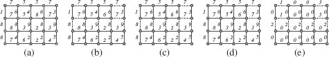
FIGURE 6.9
(a) An edge-weighted graph $\mathcal{G}$, the minima of w are depicted in bold. (b) A watershed cut represented by dashed edges; the watershed cut is equivalent to the graph ${\mathcal{G}}_0\in M\mathcal{S}F\left(ℳ\right)$ represented in bold. (c,d) two bold graphs called, respectively, ${\mathcal{G}}_1$ and ${\mathcal{G}}_2$ such that $\mathcal{T}=\langle {\mathcal{G}}_0,{\mathcal{G}}_1,{\mathcal{G}}_2\rangle$ is both an MSF hierarchy for and an uprooting by 〈M₁, M₂〉 (where M_i is the minimum of w whose altitude is i); their associated cuts are represented by dashed edges. (e) The saliency map of the MSF hierarchy $\langle {\mathcal{G}}_0,{\mathcal{G}}_1,{\mathcal{G}}_2\rangle$.

Definition 20 (MSF hierarchy, [14])

Let $ℳ=\langle M_1,\dots ,M_{\ell }\rangle$ be a sequence of pairwise distinct minima of w and let $\mathcal{T}=\langle {\mathcal{G}}_0,\dots ,{\mathcal{G}}_{\ell }\rangle$ be a sequence of subgraphs of $\mathcal{G}$. We say that $\mathcal{T}$ is an MSF hierarchy for $\mathcal{S}$ if for any i ∈ [0, ℓ], the graph ${\mathcal{G}}_i$ is an MSF rooted in $\bigsqcup \left[ℳ\left\{M_j|j\in \left[1,i\right]\right\}\right]$, and for any i ∈ [1, ℓ], we have ${\mathcal{G}}_{i-1}⊑{\mathcal{G}}_i$.

Theorem 21 ([61, 14])

Any ${\mathcal{G}}_i$ of an MSF hierarchy is a watershed cut of the geodesic reconstruction w_R where the markers are the minima rooting the MSF ${\mathcal{G}}_i$.

6.7.1    Uprootings and MSF Hierarchies

In this section, we introduce a simple transformation, called uprooting, that allows a forest ${\mathcal{G}}_1$ rooted in a graph ${\mathcal{G}}_2$ to be incrementally transformed into a forest ${\mathcal{G}}_3$ rooted in a graph ${\mathcal{G}}_4$ obtained by removing some components of ${\mathcal{G}}_2$. Through an equivalence theorem, we establish an important link between the uprooting transform and the MSF hierarchies. This result opens the way toward efficient algorithms for computing MSF hierarchies.

Let ${\mathcal{G}}_1$ be a subgraph of $\mathcal{G}$ that is spanning for $\mathcal{V}$, and let $\upsilon \in \mathcal{V}$. We denote by $C{C}_{\upsilon }\left({\mathcal{G}}_1\right)$ the component of ${\mathcal{G}}_1$ whose vertex set contains υ. Let ${\mathcal{V}}^{\prime }\subseteq \mathcal{V}$, we set $C{C}_{{\mathcal{V}}^{\prime }}\left({\mathcal{G}}_1\right)=\bigsqcup \left\{C{C}_{\upsilon }\left({\mathcal{G}}_1\right)|\upsilon \in {\mathcal{V}}^{\prime }\right\}$.

Let ${\mathcal{G}}_1⊑\mathcal{G}$, and let $e_{ij}=\left\{{\upsilon }_i,{\upsilon }_j\right\}\in ℰ$. The edge e_ij is outgoing from ${\mathcal{G}}_1$ if e_ij is made of a vertex in $\mathcal{V}\left({\mathcal{G}}_1\right)$ and of a vertex in $\overline{\mathcal{V}\left({\mathcal{G}}_1\right)}$. In the following, by abuse of notation, we write ${\mathcal{G}}_1\bigsqcup \left\{e_{ij}\right\}$ for the supremum of ${\mathcal{G}}_1$, and the graph induced by $\left\{e_{ij}\right\}:{\mathcal{G}}_1\bigsqcup \left\{e_{ij}\right\}=\left(\mathcal{V}\left({\mathcal{G}}_1\right)\cup e_{ij},ℰ\left({\mathcal{G}}_1\right)\cup \left\{e_{ij}\right\}\right)$.

Let ${\mathcal{G}}_1$, ${\mathcal{G}}_2$, and ${\mathcal{G}}_3$ be three subgraphs of $\mathcal{G}$ such that ${\mathcal{G}}_1$ is spanning for $\mathcal{V}$ and such that ${\mathcal{G}}_1\ne {\mathcal{G}}_2$. We say that ${\mathcal{G}}_2$ is an elementary uprooting of ${\mathcal{G}}_1$ by ${\mathcal{G}}_3$ if there exists an edge e of minimum weight among the edges outgoing from $C{C}_{\mathcal{V}\left({\mathcal{G}}_3\right)}\left({\mathcal{G}}_1\right)$ such that ${\mathcal{G}}_2={\mathcal{G}}_1\bigsqcup \left\{u\right\}$. We also say that ${\mathcal{G}}_2$ is an elementary uprooting of ${\mathcal{G}}_1$ by ${\mathcal{G}}_3$ if ${\mathcal{G}}_2={\mathcal{G}}_1$ and if there is no edge outgoing from $C{C}_{\mathcal{V}\left({\mathcal{G}}_3\right)}\left({\mathcal{G}}_1\right)$.

Definition 22 ([14])

Let $\mathcal{S}=\langle M_1,\dots ,M_{\ell }\rangle$ be a sequence of pairwise distinct minima of w. An uprooting by $\mathcal{S}$ is a sequence $\langle {\mathcal{G}}_0,\dots ,{\mathcal{G}}_{\ell }\rangle$ of graphs such that ${\mathcal{G}}_0\in MSF\left(ℳ\right)$ and, for any i ∈ [1, ℓ], ${\mathcal{G}}_i$ is an elementary uprooting of ${\mathcal{G}}_{i-1}$ by M_i.

Theorem 23 ([14])

Let $\mathcal{S}=\langle M_1,\dots ,M_{\ell }\rangle$ be a sequence of pairwise distinct minima of w. Let $\mathcal{T}=\langle {\mathcal{G}}_0,\dots {\mathcal{G}}_{\ell }\rangle$ be a sequence of subgraphs of $\mathcal{G}$. The sequence $\mathcal{T}$ is an MSF hierarchy for $\mathcal{S}$ if and only if the sequence $\mathcal{T}$ is an uprooting by $\mathcal{S}$.

6.7.2    Saliency Maps

The cuts of the sequence of any MSF hierarchy can be stacked to form a weighting called the saliency map. The saliency map allows us to easily assess the quality and the robustness of a hierarchical segmentation. Furthermore, it is a weighted graph, and can be further processed if needed, for example, to remove small regions unwanted in the hierarchy.

Let us give a precise defition of the saliency map [56, 14]. We first need to define, for a graph $\mathcal{G}$, the map ϕ as $\varphi \left(\mathcal{G}\right)=\bigsqcup \left\{{\alpha }_2\left({\mathcal{G}}_i\right)|{\mathcal{G}}_i\text{is}\text{a}\text{component}\text{of}\mathcal{G}\right\}$. In other words, $\varphi \left(\mathcal{G}\right)$ is the union of all the graphs induced by the connected components of $\mathcal{G}$. It is easy to see that ϕ is an opening.

Let $ℳ=\langle M_1,\dots ,M_{\ell }\rangle$ be a sequence of pairwise distinct minima of w and Let $\mathcal{T}=\langle {\mathcal{G}}_0,\dots {\mathcal{G}}_{\ell }\rangle$ be a MSF hierarchy for $ℳ$. The saliency map s for $\mathcal{T}$ is the map such that for any $e_{ij}\in ℰ$, either s_ij = k if there exists k such that k is the lowest number satisfying $e_{ij}\in \varphi \left({\mathcal{G}}_k\right)$ or s_ij = l + 1 if it does not exists any ${\mathcal{G}}_k$ such that $e_{ij}\in \varphi \left({\mathcal{G}}_k\right)$. Observe, in particular, that if $e_{ij}\in ℰ\left(\varphi \left({\mathcal{G}}_0\right)\right)$, s_ij = 0, and that $s\left[\lambda \right]=\varphi \left({\mathcal{G}}_{\lambda }\right)$ for λ ∈ {0, ⋯, l}.

Under the term of ultrametric watershed, one can give a computable definition to saliency maps, allowing to show the equivalenve between the set of hierarchical segmentations and the set of saliency maps [60].

6.7.3    Application to Image Segmentation

To use the framework in practice, we have to design an order on the minima of w. Let μ be an attribute on ${\mathcal{C}}_{ℰ}^{<}$ (i.e., a function from ${\mathcal{C}}_{ℰ}^{<}$ to $ℝ$ that is increasing on ${\mathcal{C}}_{ℰ}^{<}$) such as the area, the volume, or the height. We compute an extinction measure [62, 63] μ_e to each minima of w by first definining a strict total order relation ≺ on the set of minima (based for example on the altitude of each minimum) such that M₀ ≺ M₁ ≺ ⋯ ≺ M_l; then we set μ_e(M₀) = ∞ and

$\begin{array}{rr}\hfill {\mu }_e\left(M_i\right)=& \hfill \min \{\mu \left(\left[\lambda ,C\right]\right)|\left[\lambda ,C\right]\in {\mathcal{C}}_{ℰ}^{<},\\ \hfill & \hfill \text{there}\text{exists}{M}_j\text{a}\text{minimum}\text{of}w,M_j\prec M_i\}\end{array}$

(6.5)

The map μ_e will define the order ≺_e of the sequence for the hierachy of MSF: M_i ≺_e M_j whenever μ_e(M_e) < μ_e(M_j).

Other choices for the ordering are possible: for example, waterfall [64], that consists in computing a sequence of watersheds of watersheds, each step leading to a drastic reduction in the number of basins. Another interesting ordering is done by optimization [57]). Let us consider a two-term-based energy function of the form λC + D, where D is a goodness-of-fit term and C is a regularization term. Finding an optimum of this function is NP-hard in the general case. On the other hand, on a hierarchy (hence, on a watershed cut), when the goodness-of-fit term decreases with the fineness of the partitions, and, inversely, that the regularization term increases with this fineness, we can show that finding an optimum can be done in linear time, by dynamic programming. Such an optimization is an efficient way to control the flooding, which is stopped when the optimum is reached. Varying the λ parameter allows us to obtain a complete hierarchy of segmentations.

Figure 6.10(b), (c), and (d) illustrates some saliency maps on the image of Figure 6.10a. The underlying graph is the one induced by the 4-adjacency relation whose edges are weighted by a simple color gradient (maximum, over the RGB channels, of the absolute differences of pixel values). The minima are ordered, thanks to extinction values [62] related to depth, volume, and color consistency.

6.8    Optimization and the Power Watershed

In this section, we review the Power Watershed framework [15] (see also Leo Grady’s chapter, this book). In the previous sections dealing with watershed cuts, the weights encode a dissimilarity such as a gradient. Classicaly, in the context of segmentation and clustering applications based on optimization, the weights encode affinity such that vertices connected by an edge with high weight are considered to be strongly connected and edges with a low weight represent nearly disconnected vertices. One common choice for generating weights from image intensities is to set a Gaussian weighting such as

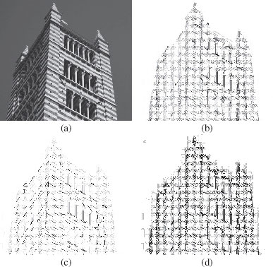
FIGURE 6.10
Illustration of saliencies of watershed cuts (original picture (a) from koakoo: http://blog.photos-libres.fr/).

$w_{ij}=\exp \left(-\beta {\left(\nabla I\right)}^2\right),$

(6.6)

where ∇I is the normalized gradient of the image I. The gradient for a grey level image is I_i − I_j. As the weights are inverted, the maxima are considered instead of minima, and a thalweg is computed instead of watershed. A thalweg is the deepest continuous line along a valley. In the rest of the paper, we continue to use by convention the term “watershed” instead of “thalweg”.

Given foreground F and background B seeds, and p, q two real positive values, the energy presented for binary segmentation in [15] is given by

$x^{\star pq}=\arg \underset{x}{\min }{\displaystyle \sum _{e_{ij}\in E}{w}_{ij}^p{\left|x_i-x_j\right|}^q\text{s}\text{.t}\text{.}x\left(F\right)}=1,x\left(B\right)=0.$

(6.7)

In this energy, w_ij can be interpreted as a weight enforcing a regularization of the contours, such that any (usually unwanted) high-frequency content is penalized in x. The energy defined in (6.7) essentially forces x to remain smooth within the object, while allowing it to vary quickly close to point clusters near the boundary of the object. The data constraints enforce fidelity of x to a specified configuration, taking the values zero and one as the reconstructed object indicator. Observe that the values of x may not necessarily be binary when the value of q is strictly greater than one.

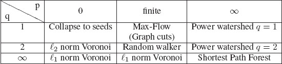
TABLE 6.1
The generalized scheme of [15] for image segmentation includes several popular segmentation algorithms as special cases of the parameters p and q. The power watershed may be optimized efficiently with a maximum spanning forest calculation.

The different values of p and q lead to different algorithms for optimizing the energy. Those algorithms form the underpinning for many of the advanced image segmentation methods in the literature. Table 6.1 gives a reference for the different algorithms generated by various values of p and q. The limit cases are the limit of the minimizers of Equation (6.7), e.g., the case p → ∞ reads

$x^{\star q}=\underset{p\to \infty }{\lim }{x}^{\star pq}.$

(6.8)

Let us highlight the main choices for those parameters.

•  When the power on the weight, p, is finite, and the exponent q = 1, we recover [61] the Max-Flow (Graph Cuts) energy which can be optimized by a max flow algorithm.

•  When q = 2, we obtain a combinatorial Dirichlet problem also known as the random walker problem [65].

•  When q and p converge toward infinity with the same speed, then [66] a solution to (6.8) can be computed by the shortest path (geodesics) algorithm [6, 67].

•  As described in [15], by raising the power p toward infinity, and varying the power q, we obtain a family of segmentation models, which we refer to as power watershed, and that we detailed below.

A primary advantage of power watershed with varying q is that the main computational burden of these algorithms depends on an MSF computation, which is extremely efficient [68]. For example, interpreted from the standpoint of the Gaussian weighting function in (6.6), it is clear that we may associate β = p to understand that the watershed equivalence comes from operating the weighting function in a particular parameter range. In the case q = 1, an important insight from this connection is that above some value of β we can replace the expensive max-flow computation with an efficient maximum spanning forest computation.

Let us review some important theoretical results. First, we highlight that the cut obtained when minimizing the energy (6.8) is a watershed cut [13], and thus a maximum spanning forests [13] (MSF). Let x^⋆ be a solution to (6.8) and s be the segmentation result defined as s_i = 1 if $x_i^{\star }\ge \frac{1}{2}$, 0 if $x_i^{\star }<\frac{1}{2}$. The set of edges e_ij such that s_i ≠ s_j is a q-cut.

Theorem 24 ([15])

For q ≥ 1, any q-cut is a watershed cut of the (geodesically) reconstructed weights.

Furthermore, if every connected component of $ℳ$ contains at least a vertex of B ∪ F, and q ≥ 1, then any q-cut when p → ∞ is an MSF cut for w.

Algorithm 1: Power watersheds algorithm p → ∞, q > 1

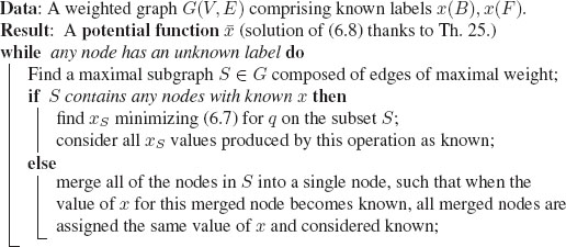
An algorithm is presented in Algorithm 1 to optimize the (unique) watershed that optimizes the energy for q > 1 and p → ∞. The case of parameter p → ∞ is particularly interesting.

1.  The power watershed algorithm in the case q > 1 has a well-defined behavior in the absence or lack of weight information (presence of plateaus); indeed, as the energy is strictly convex, the solution to (6.8) is unique.

2.  The worst-case complexity of the power watershed algorithm in the case p → ∞ is given by the cost of optimizing (6.7) for the given q. In the best-case scenario (all weights have unique values), the power watershed algorithm has the same asymptotic complexity as the algorithm used for a MSF computation (quasi-linear). In practical applications where the plateaus have a size less than some fixed value K, then the complexity of the power watershed algorithm matches the quasi-linear complexity of the standard watershed-cut algorithm.

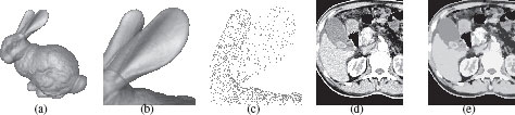
FIGURE 6.11
Two applications of power watershed. (a-c) Shape fitting using power watershed [69]. (a) reconstructed bunny. (b) A close-up on one of the ears. (c) A close-up on the set of original scanned noisy points measurements. (d-e) Filtering of a liver image by anisotropic diffusion driven by power watershed [70]. In (e) noise and small vessels are both removed from (d), leading to a result which may be used as a first step before segmentation.

The main properties of Algorithm 1 (with q ≥ 1) are summarized in the following theorem. This theorem states that the energy found by the algorithm is the correct one, i.e. $x^{\star q}=\overline{x}$, and that furthermore, the computed cut is a MSF cut.

Theorem 25 ([15])

If q > 1, the potential x^⋆ obtained by minimizing the energy of (6.7) subject to the boundary constraints converges toward the potential $\overline{x}$ obtained by Algorithm 1 as p → ∞.

Furthermore, for any q ≥ 1, the cut C defined by the segmentation s computed by Algorithm 1 is an MSF cut for w.

6.8.1    Applications

Minimizing exactly the energy E_{1, 1} is possible by using the graph cuts (i.e., q = 1) algorithm in the case of two labels, but is NP-hard if constraints impose more than two different labels. However, the other algorithms presented in the framework (and, in particular, the watershed cuts and the power watershed) can efficiently perform seeded segmentation with as many labels as desired [15]. As several examples of segmentation have already been shown in this chapter, we rather highlight two other applications that take advantage the unique optimization characteristics of the power watershed.

The first example is shape fitting. Surface reconstruction from a set of noisy point measurements has been a well studied problem over the last decades. Recently, variational [71, 72] and discrete optimization [73] approaches have been applied to solve it, demonstrating good robustness to outliers thanks to a global energy minimization scheme. In [69], Couprie et al. use the power watershed framework to derive a specific watershed algorithm for surface reconstruction. The proposed algorithm is fast, robust to marker placement, and produces smooth surfaces. Figure 6.11(a–c) shows a surface reconstructed from noisy scanned dot sets using the power watershed algorithm.

The second example deals with filtering. In [70], Couprie et al. reformulate the problem of anisotropic diffusion as an L₀ optimization problem, and show that power watersheds are able to optimize this energy quickly and effectively. This study paves the way for using the power watershed as a useful general-purpose minimizer in many different computer vision contexts. An example of such an L₀ optimization is presented in Figures 6.11(d–e).

6.9    Conclusion

We have presented in this paper some applications of mathematical morphology to weighted graphs. The translation of the abstract framework of lattices to graphs allows us to obtain morphological operators thinner (in the sense that they process smaller details) than the usual ones commonly defined only on the vertices. We have shown how to filter an image using connected filters based on a tree representation of the image. We have exhibited the links between watersheds and minimum spanning trees, allowing us to make the equivalence between hierarchical segmentation based on watershed cuts and minimum spanning trees. We conclude the chapter by exploring links between the morphological and the optimization approaches.

For practical applications, we want to stress the importance of having a framework with an open-source generic implementation of existing algorithms, not limited to the pixel framework, but also able to deal transparently with edges, or, more generally, with graphs and complexes [74].

Bibliography

[1]  G. Matheron, Random sets and integral geometry. New York: John Wiley & Sons, 1975.

[2]  J. Serra, Image analysis and mathematical morphology. London, U.K.: Academic Press, 1982.

[3]  J. Serra, Ed., Image analysis and mathematical morphology. Volume 2: Theoretical advances. London, U.K.: Academic Press, 1988.

[4]  L. Vincent, “Graphs and mathematical morphology,” Signal Processing, vol. 16, pp. 365–388, 1989.

[5]  H. Heijmans and L. Vincent, “Graph morphology in image analysis,” in Mathematical morphology in image processing, E. Dougherty, Ed. New York: Marcel Dekker, 1993, vol. 34, ch. 6, pp. 171–203.

[6]  A. X. Falcão, R. A. Lotufo, and G. Araujo, “The image foresting transformation,” IEEE PAMI, vol. 26, no. 1, pp. 19–29, 2004.

[7]  F. Meyer and R. Lerallut, “Morphological operators for flooding, leveling and filtering images using graphs,” in Graph-based Representations in Pattern Recognition (GbRPR’07), vol. LNCS 4538, 2007, pp. 158–167.

[8]  F. Meyer and J. Angulo, “Micro-viscous morphological operators,” in Mathematical Morphology and its Application to Signal and Image Processing (ISMM 2007), 2007, pp. 165–176.

[9]  V.-T. Ta, A. Elmoataz, and O. Lézoray, “Partial difference equations over graphs: Morphological processing of arbitrary discrete data,” in ECCV 2008, ser. Lecture Notes in Computer Science, D. Forsyth, P. Torr, and A. Zisserman, Eds. Springer Berlin / Heidelberg, 2008, vol. 5304, pp. 668–680.

[10]  J. Cousty, L. Najman, and J. Serra, “Some morphological operators in graph spaces,” in International Symposium on Mathematical Morphology 2009, ser. LNCS, vol. 5720. Springer Verlag, Aug. 2009, pp. 149–160.

[11]  I. Bloch and A. Bretto, “Mathematical morphology on hypergraphs: Preliminary definitions and results,” in Discrete Geometry for Computer Imagery, ser. Lecture Notes in Computer Science, I. Debled-Rennesson, E. Domenjoud, B. Kerautret, and P. Even, Eds. Springer Berlin / Heidelberg, 2011, vol. 6607, pp. 429–440.

[12]  F. Dias, J. Cousty, and L. Najman, “Some morphological operators on simplicial complexes spaces,” in DGCI 2011, ser. LNCS, no. 6607. Springer, 2011, pp. 441–452.

[13]  J. Cousty, G. Bertrand, L. Najman, and M. Couprie, “Watershed Cuts: Minimum Spanning Forests and the Drop of Water Principle,” IEEE PAMI, vol. 31, no. 8, pp. 1362–1374, Aug. 2009.

[14]  J. Cousty and L. Najman, “Incremental algorithm for hierarchical minimum spanning forests and saliency of watershed cuts,” in ISMM 2011, ser. LNCS, no. 6671, 2011, pp. 272–283.

[15]  C. Couprie, L. Grady, L. Najman, and H. Talbot, “Power Watersheds: A Unifying Graph Based Optimization Framework,” IEEE Transactions on Pattern Analysis and Machine Intelligence, vol. 33, no. 7, pp. 1384–1399, July 2011, http://doi.ieeecomputersociety.org/10.1109/TPAMI.2010.200. [Online]. Available: http://powerwatershed.sourceforge.net/

[16]  P. Soille, Morphological Image Analysis. Springer-Verlag, 1999.

[17]  L. Najman and H. Talbot, Eds., Mathematical morphology: from theory to applications. ISTE-Wiley, June 2010.

[18]  Nesetril, Milkova, and Nesetrilova, “Otakar Boruvka on Minimum Spanning Tree problem: Translation of both the 1926 papers, comments, history,” DMATH: Discrete Mathematics, vol. 233, 2001.

[19]  G. Choquet, “étude de certains réseaux de routes,” Comptes-rendus de l’Acad. des Sciences, pp. 310–313, 1938.

[20]  C. Zahn, “Graph-theoretical methods for detecting and descibing Gestalt clusters,” IEEE Transactions on Computers, vol. C-20, no. 1, pp. 99–112, 1971.

[21]  O. J. Morris, M. d. J. Lee, and A. G. Constantinides, “Graph theory for image analysis: an approach based on the shortest spanning tree,” IEE Proc. on Communications, Radar and Signal, vol. 133, no. 2, pp. 146–152, 1986.

[22]  F. Meyer, “Minimum spanning forests for morphological segmentation,” in Procs. of the second international conference on Mathematical Morphology and its Applications to Image Processing, September 1994, pp. 77–84.

[23]  P. Felzenszwalb and D. Huttenlocher, “Efficient graph-based image segmentation,” International Journal of Computer Vision, vol. 59, pp. 167–181, 2004.

[24]  L. Vincent and P. Soille, “Watersheds in digital spaces: An efficient algorithm based on immersion simulations,” IEEE PAMI, vol. 13, no. 6, pp. 583–598, June 1991.

[25]  G. Birkhoff, Lattice Theory, ser. American Mathematical Society Colloquium Publications. American Mathematical Society, 1995, vol. 25.

[26]  C. Ronse and J. Serra, “Algebric foundations of morphology,” in Mathematical Morphology, L. Najman and H. Talbot, Eds. ISTE-Wiley, 2010, pp. 35–79.

[27]  P. Salembier and J. Serra, “Flat zones filtering, connected operators, and filters by reconstruction,” IEEE TIP, vol. 4, no. 8, pp. 1153–1160, Aug 1995.

[28]  C. Ronse, “Set-theoretical algebraic approaches to connectivity in continuous or digital spaces,” JMIV, vol. 8, no. 1, pp. 41–58, 1998.

[29]  U. Braga-Neto and J. Goutsias, “Connectivity on complete lattices: new results,” Comput. Vis. Image Underst., vol. 85, no. 1, pp. 22–53, 2002.

[30]  G. K. Ouzounis and M. H. Wilkinson, “Mask-based second-generation connectivity and attribute filters,” IEEE PAMI, vol. 29, no. 6, pp. 990–1004, 2007.

[31]  R. K. Gabriel and R. R. Sokal, “A new statistical approach to geographic variation analysis,” Systematic Zoology, vol. 18, no. 3, pp. 259–278, Sep. 1969.

[32]  P. Salembier, A. Oliveras, and L. Garrido, “Anti-extensive connected operators for image and sequence processing,” IEEE TIP, vol. 7, no. 4, pp. 555–570, April 1998.

[33]  L. Najman and M. Couprie, “Building the component tree in quasi-linear time,” IEEE TIP, vol. 15, no. 11, pp. 3531–3539, 2006.

[34]  P. Salembier and L. Garrido, “Binary partition tree as an efficient representation for image processing, segmentation and information retrieval,” IEEE Transactions on Image Processing, vol. 9, no. 4, pp. 561–576, Apr. 2000.

[35]  V. Caselles and P. Monasse, Geometric Description of Images as Topographic Maps, ser. Lecture Notes in Computer Science. Springer, 2010, vol. 1984.

[36]  P. Salembier, “Connected operators based on tree pruning strategies,” in Mathematical morphology:from theory to applications, L. Najman and H. Talbot, Eds. ISTE-Wiley, 2010, pp. 179–198.

[37]  J. Benzécri, L’Analyse des données: la Taxinomie. Dunod, 1973, vol. 1.

[38]  B. Leclerc, “Description combinatoire des ultramétriques,” Mathématique et sciences humaines, vol. 73, pp. 5–37, 1981.

[39]  N. Jardine and R. Sibson, Mathematical taxonomy. Wiley, 1971.

[40]  J. Gower and G. Ross, “Minimum spanning tree and single linkage cluster analysis,” Appl. Stats., vol. 18, pp. 54–64, 1969.

[41]  J. B. Kruskal, “On the shortest spanning subtree of a graph and the traveling salesman problem,” Proceedings of the American Mathematical Society, vol. 7, pp. 48–50, February 1956.

[42]  F. Meyer and S. Beucher, “Morphological segmentation,” JVCIR, vol. 1, no. 1, pp. 21–46, Sept. 1990.

[43]  S. Beucher and F. Meyer, “The morphological approach to segmentation: the watershed transformation,” in Mathematical morphology in image processing, ser. Optical Engineering, E. Dougherty, Ed. New York: Marcel Dekker, 1993, vol. 34, ch. 12, pp. 433–481.

[44]  L. Najman and M. Schmitt, “Watershed of a continuous function,” Signal Processing, vol. 38, no. 1, pp. 99–112, 1994.

[45]  J. B. T. M. Roerdink and A. Meijster, “The watershed transform: Definitions, algorithms and parallelization strategies,” Fundamenta Informaticae, vol. 41, no. 1–2, pp. 187–228, 2001.

[46]  G. Bertrand, “On topological watersheds,” JMIV, vol. 22, no. 2–3, pp. 217–230, May 2005.

[47]  J. Cousty, G. Bertrand, L. Najman, and M. Couprie, “Watershed cuts: thinnings, shortest-path forests and topological watersheds,” IEEE PAMI, vol. 32, no. 5, pp. 925–939, 2010.

[48]  F. Meyer, “Topographic distance and watershed lines,” Signal Processing, vol. 38, no. 1, pp. 113–125, July 1994.

[49]  P. Soille and C. Gratin, “An efficient algorithm for drainage networks extraction on DEMs,” Journal of Visual Communication and Image Representation, vol. 5, no. 2, pp. 181–189, June 1994.

[50]  S. Philipp-Foliguet, M. Jordan, L. Najman, and J. Cousty, “Artwork 3D Model Database Indexing and Classification,” Pattern Recogn., vol. 44, no. 3, pp. 588–597, Mar. 2011.

[51]  L. J. Grady and J. R. Polimeni, Discrete Calculus: Applied Analysis on Graphs for Computational Science, 1st ed. Springer, Aug. 2010.

[52]  P. J. Basser, J. Mattiello, and D. LeBihan, “MR diffusion tensor spectroscopy and imaging.” Biophys. J., vol. 66, no. 1, pp. 259–267, 1994.

[53]  V. Arsigny, P. Fillard, X. Pennec, and N. Ayache, “Log-Euclidean metrics for fast and simple calculus on diffusion tensors,” Magnetic Resonance in Medicine, vol. 56, no. 2, pp. 411–421, August 2006.

[54]  J. Cousty, L. Najman, M. Couprie, S. Clément-Guinaudeau, T. Goissen, and J. Garot, “Segmentation of 4D cardiac MRI: automated method based on spatio-temporal watershed cuts,” IVC, vol. 28, no. 8, pp. 1229–1243, Aug. 2010.

[55]  F. Meyer, “The dynamics of minima and contours,” in Mathematical Morphology and its Applications to Image and Signal Processing, P. Maragos, R. Schafer, and M. Butt, Eds. Boston: Kluwer, 1996, pp. 329–336.

[56]  L. Najman and M. Schmitt, “Geodesic saliency of watershed contours and hierarchical segmentation,” IEEE PAMI, vol. 18, no. 12, pp. 1163–1173, December 1996.

[57]  L. Guigues, J. P. Cocquerez, and H. L. Men, “Scale-sets image analysis,” IJCV, vol. 68, no. 3, pp. 289–317, 2006.

[58]  P. A. Arbeláez and L. D. Cohen, “A metric approach to vector-valued image segmentation,” IJCV, vol. 69, no. 1, pp. 119–126, 2006.

[59]  F. Meyer and L. Najman, “Segmentation, minimum spanning tree and hierarchies,” in Mathematical Morphology: from theory to application, L. Najman and H. Talbot, Eds. London: ISTE-Wiley, 2010, ch. 9, pp. 229–261.

[60]  L. Najman, “On the equivalence between hierarchical segmentations and ultrametric watersheds,” Journal of Mathematical Imaging and Vision, vol. 40, no. 3, pp. 231–247, July 2011, arXiv:1002.1887v2. [Online]. Available: http://www.laurentnajman.org

[61]  C. Allène, J.-Y. Audibert, M. Couprie, and R. Keriven, “Some links between extremum spanning forests, watersheds and min-cuts,” IVC, vol. 28, no. 10, pp. 1460–1471, Oct. 2010.

[62]  C. Vachier and F. Meyer, “Extinction value: a new measurement of persistence,” in IEEE Workshop on Nonlinear Signal and Image Processing, 1995, pp. 254–257.

[63]  G. Bertrand, “On the dynamics,” IVC, vol. 25, no. 4, pp. 447–454, 2007.

[64]  S. Beucher, “Watershed, hierarchical segmentation and waterfall algorithm,” in Mathematical Morphology and its Applications to Image Processing, J. Serra and P. Soille, Eds. Kluwer Academic Publishers, 1994, pp. 69–76.

[65]  L. Grady, “Random walks for image segmentation,” IEEE PAMI, vol. 28, no. 11, pp. 1768–1783, 2006.

[66]  A. K. Sinop and L. Grady, “A seeded image segmentation framework unifying graph cuts and random walker which yields a new algorithm,” in Proc. of ICCV’07, 2007.

[67]  G. Peyre, M. Pechaud, R. Keriven, and L. Cohen, “Geodesic methods in computer vision and graphics,” Foundations and Trends in Computer Graphics and Vision, vol. 5, no. 3-4, pp. 197–397, 2010. [Online]. Available: http://hal.archives-ouvertes.fr/hal-00528999/

[68]  B. Chazelle, “A minimum spanning tree algorithm with inverse-Ackermann type complexity,” Journal of the ACM, vol. 47, pp. 1028–1047, 2000.

[69]  C. Couprie, X. Bresson, L. Najman, H. Talbot, and L. Grady, “Surface reconstruction using power watershed,” in ISMM 2011, ser. LNCS, no. 6671, 2011, pp. 381–392.

[70]  C. Couprie, L. Grady, L. Najman, and H. Talbot, “Anisotropic Diffusion Using Power Watersheds,” in International Conference on Image Processing (ICIP’10), Sept. 2010, pp. 4153–4156.

[71]  T. Goldstein, X. Bresson, and S. Osher, “Geometric applications of the Split Bregman Method: Segmentation and surface reconstruction,” UCLA, Computational and Applied Mathematics Reports, Tech. Rep. 09-06, 2009.

[72]  J. Ye, X. Bresson, T. Goldstein, and S. Osher, “A fast variational method for surface reconstruction from sets of scattered points,” UCLA, Computational and Applied Mathematics Reports, Tech. Rep. 10-01, 2010.

[73]  V. Lempitsky and Y. Boykov, “Global Optimization for Shape Fitting,” in Proc. IEEE Conference on Computer Vision and Pattern Recognition (CVPR), Minneapolis, USA, 2007.

[74]  R. Levillain, T. Géraud, and L. Najman, “Why and How to Design a Generic and Efficient Image Processing Framework: The Case of the Milena Library,” in 17th International Conference on Image Processing, 2010, pp. 1941–1944.