4

A Parametric Maximum Flow Approach for Discrete Total Variation Regularization

Chambolle Antonin

CMAP, Ecole Polytechnique, CNRS
F-91128 Palaiseau, France

Email: [email protected]

Jérôme Darbon

CMLA, ENS Cachan, CNRS, PRES UniverSud
F-94235 Cachan, France

Email: [email protected]

CONTENTS

4.1    Introduction

4.2    Idea of the approach

4.3    Numerical Computations

4.3.1    Binary Optimization

4.3.2    Discrete Total Variations optimization

4.4    Applications

Bibliography

4.1    Introduction

In this chapter, we consider the general reconstruction problem with total variation (TV) that takes the following form

E(u) = F(u)+ λJ(u)E(u) = F(u)+ λJ(u)$E\left(u\right)=F\left(u\right)+\text{λ}J\left(u\right)$

with m ≤ u ≤ M, and where F and J, respectively, correspond to the data fidelity and the discrete total variation terms (to be defined later). We shall consider the three following cases for the data fidelity term F, which are widely used in image processing:

$F\left(u\right)=\{\begin{array}{l}\frac{1}{2}{\Vert Au-f\Vert }^2\hfill \\ \frac{1}{2}{\Vert u-f\Vert }^2\hfill \\ \frac{1}{2}{\Vert u-f\Vert }_1\hfill \end{array}$

(4.1)

where f is the observed data.

The most widely used approaches nowadays for performing nonsmooth optimization rely on variants of the proximal point algorithm [1, 2] or proximal splitting techniques [3, 4, 5, 6]. It is, therefore, an interesting problem to compute the proximity operator [1] of common regularizers for inverse problems in imaging. In this chapter we address the problem of computing the proximity operator of the discrete TV and we describe a few elementary imaging applications. Note that the techniques we are considering here, which rely on an ordering of the values at each pixel, work only for scalar-valued (grey) images and cannot be extended to vector-valued (color) data.

It was firstly observed by Picard and Ratliff in [7] that Boolean Markovian energies with second-order cliques can be mapped to a network flow on a oriented graph with a source and a sink (and minimizing the energy corresponds to computing the s,t-minimum-cut or solving maximum-flow by duality). This technique was used by Greig et al. in [8] to estimate the quality of the maximum a posteriori estimator of ferromagnetic Ising models for binary image restoration. Then, it was observed that solving a series of the above problems where source-node capacities are gradually increasing can be optimized with the time complexity of a single maximum-flow using a parametric maximum-flow approach [9, 10] (provided the number parameter is less than the number of pixels). A further improvement has been proposed by [11] who shows how to compute efficiently an exact solution, provided that the data fidelity term is separable and that the space of solutions is a discrete space.

This last approach has been rediscovered, and in some sense extended (in particular, to more general submodular interaction energies) by the authors of [12, 13, 14, 15, 16, 17, 18]. In particular, they describe in [15] a method which solves “exactly” (up to machine precision) the proximity operator of some discrete total variation energies. In the chapter we will describe with further details this technique along with some basic image processing applications.

Notations

In this paper we shall consider that an image is defined on a discrete grid Ω. The gray-level value of the image $u\in {ℝ}^{\Omega }$ at the site i ∈ Ω is referred to as $u_i\in ℝ$.

A very general “discrete total variation” problem we can solve with a network-flow-based approach has the following form:

$J\left(u\right)={\displaystyle \sum _{i\ne j}{w}_{ij}{\left(u_j-u_i\right)}^{+}},$

(4.2)

where x⁺ = max(x, 0) is the nonnegative part of $x\in ℝ$. Here, w_ij are nonnegative values that weight each interaction. For the sake of clarity we shall assume that w_ij = w_ji, and thus we consider discrete TV of the form

$J\left(u\right)={\displaystyle \sum _{\left\{i,j\right\}}{w}_{ij}\left|u_j-u_i\right|},$

(4.3)

where each interaction (i, j) appears only once in the sum. In practice, the grid is endowed with a neighborhood system and the weights w_ij are nonnegative only when i and j are neighbors. Two neighboring sites i and j are denoted by i ~ j.

For instance, one common example is to consider a regular 2D grid endowed with the 4-connectivity (i.e., 4 nearest neighbors) where the weights are all set to 1. In that case J is an approximation of the l₁-anisotropic total variation that formally writes as ${\displaystyle \int \left(\left|{\partial }_{x}u\right|+\left|{\partial }_{y}u\right|\right)}$. Less anisotropic versions can be obtained by considering more neighbors (with appropriate weights). Observe that we cannot tackle with our techniques the minimization of standard approximations of the isotropic TV written formally as ${\displaystyle \int \sqrt{{\left|{\partial }_{x}u\right|}^2+{\left|{\partial }_{y}u\right|}^2}}$, as for instance in [19, 20]. Finally, note that one can extend the proposed approach to some higher-order interaction terms without too much effort by adding some internal nodes; We refer the reader to [15] for more details.

In the next section, we describe the parametric maximum approach for computing the proximity operator of the discrete TV. We follow with more details our description in [15] of the approach essentially due to Hochbaum [11]. Then we describe some applications.

4.2    Idea of the approach

Our goal is to minimize the energy $J\left(u\right)+\frac{1}{2}{\Vert u-g\Vert }^2=J\left(u\right)+\frac{1}{2}{{\displaystyle {\sum }_{i\in \Omega }\left(u_i-g_i\right)}}^2$, or similar energies, where J has the form (4.3) and $g\in {ℝ}^{\Omega }$ is given.

Here, the general form we are interested in is $J\left(u\right)+{\displaystyle {\sum }_i\psi \left(u_i\right)}$, where ψ_i is a convex function (in our case, ${\psi }_i\left(z\right)=\frac{1}{2}{\left(z-g_i\right)}^2$ with i ∈ Ω). The essential point here is that the derivative of ψ_i is nondecreasing. Nonseparable data terms (such as ‖Au – g−²) will be considered in Section 4.4.

In what follows, we will denote by ${{\psi }^{\prime }}_i\left(z\right)$ the left derivative of ψ_i at z. All that follows would work in the same way if we considered the right-derivative, or any monotonous selection of the subgradient: the important point here is that ${{\psi }^{\prime }}_i\left(z\right)\le {{\psi }^{\prime }}_i\left(z^{\prime }\right)$ for all z ≤ z′.

For each $z\in ℝ$, we consider the minimization problem

$\begin{array}{cc}\underset{\theta \in {\left\{0,1\right\}}^{\Omega }}{\min }J\left(\theta \right)+{\displaystyle \sum _{i\in \Omega }{{\psi }^{\prime }}_i\left(z\right){\theta }_i}& \left(P_z\right)\end{array}$

The following comparison lemma is classical:

Lemma 4.2.1

Let z > z′, i, ∈ Ω and assume that ${{\psi }^{\prime }}_i\left(z\right)>{{\psi }^{\prime }}_i\left(z^{\prime }\right)$ (which holds for instance if ψ_i is strictly convex): then, ${\theta }_i^z\le {\theta }_i^{z^{\prime }}$.

An easy proof is found for instance in [15]: the idea is to compare the energy of θ^z in (P_z) with the energy of θ^z ∧ θ^z′, and the energy of θ^z′ in (P_z′) with the energy of θ^z ∨ θ^z′, and sum both inequalities. Then, we get rid of the terms involving J thanks to its submodularity:

$J\left({\theta }^z\wedge {\theta }^{z^{\prime }}\right)+J\left({\theta }^z\vee {\theta }^{z^{\prime }}\right)\le J\left({\theta }^z\right)+J\left({\theta }^{z^{\prime }}\right)$

(4.4)

which is the essential property upon which is based most of the analysis of this chapter [21, 15, 22].

Remark 4.2.2

Now, if the ψ_i are not strictly convex, it easily follows from Lemma 4.2.1 that the conclusion remains true provided either θ^z is the minimal solution of (P_z), or θ^z′ the maximal solution of (P_z′). Note that these smallest and largest solutions are well-defined since the energies of (P_z) are submodular.

To check this, we introduce for ε > 0 small a solution θ^{z, ε} to

$\underset{\theta \in {\left\{0,1\right\}}^{\Omega }}{\min }J\left(\theta \right)+{\displaystyle \sum _{i\in \Omega }\left({{\psi }^{\prime }}_i\left(z\right)+\epsilon \right){\theta }_i}.$

Then, the Lemma guarantees that ${\theta }_i^{z,\epsilon }\le {\theta }_i^{z^{\prime }}$ for all i, as soon as z′ ≤ z. In the limit, we easily check that ${\underset{\_}{\theta }}_i^z={\lim }_{\epsilon \to 0}{\theta }_i^{z,\epsilon }={\sup }_{\epsilon \to 0}{\theta }_i^{z,\epsilon }$ is a solution of (P_z), still satisfying ${\underset{\_}{\theta }}_i^z\le {\theta }_i^{z^{\prime }}$ for any i ∈ Ω and z′ ≤ z. This shows both that ${\underset{\_}{\theta }}^z$ is the smallest solution to (P_z), and that it is below any solution to (P_z′) with z′ < z, which is the claim of Remark 4.2.2.

We will also denote by ${\overline{\theta }}^z$ the maximal solution of (P_z). This allows us to define two vectors $\underset{\_}{u}$ and $\overline{u}$ as the following for any i ∈ Ω

$\{\begin{array}{l}{\underset{\_}{u}}_i=\sup \left\{z,{\underset{\_}{\theta }}_i^z=1\right\},\hfill \\ {\overline{u}}_i=\sup \left\{z,{\overline{\theta }}_i^z=1\right\}.\hfill \end{array}$

(4.5)

Let us now show the following result:

Proposition 4.2.3

We have that $\underset{\_}{u}$ and $\overline{u}$ are, respectively, the minimal and maximal solutions of

$\underset{u}{\min }\left(J\left(u\right)+{\displaystyle \sum _{i\in \Omega }{\psi }_i\left(u_i\right)}\right).$

(4.6)

Proof: The proof relies on the (discrete, and straightforward) “co-area formula”, which states that

$J\left(u\right)={\displaystyle \underset{-\infty }{\overset{\infty }{\int }}J\left({\chi }_{\left\{u>z\right\}}\right)dz},$

(4.7)

and simply follows from the remark that for any $a,b\in ℝ,\left|a-b\right|={\displaystyle {\int }_{ℝ}\left|{\chi }_{\left\{a>s\right\}}-{\chi }_{\left\{b>s\right\}}\right|ds}$.

Let us first choose for any z a solution θ^z of (P_z), and let

$u_i=\sup \left\{z,{\theta }_i^z=1\right\}.$

(4.8)

We first observe that for any z, $\left\{i:u_i>z\right\}\subseteq \left\{i:{\theta }_i^z=1\right\}\subseteq \left\{i:u_i>s\right\}$, so that, letting $\mathcal{U}=\left\{u_i:i\in \Omega \right\}$ we have that for any $z\in ℝ\mathcal{U}$,

$\left\{i:u_i>z\right\}=\left\{i:{\theta }_i^z=1\right\}=\left\{i:u_i>z\right\}$

(4.9)

so that almost all level sets of u are minimizers of (P_z). Then, if $v\in {ℝ}^{\Omega }$ and m ≤ min {u_i, υ_i : i ∈ Ω}, we find that

$\begin{array}{l}J\left(u\right)+{\displaystyle \sum _{i\in \Omega }{\psi }_i\left(u_i\right)}={\displaystyle \underset{m}{\overset{\infty }{\int }}J\left({\chi }_{\left\{u>z\right\}}\right)}dz+{\displaystyle \sum _{i\in \Omega }{\displaystyle \underset{m}{\overset{\infty }{\int }}{{\psi }^{\prime }}_i\left(z\right){\chi }_{\left\{u_i>z\right\}}dz}}\hfill \\ ={\displaystyle \underset{m}{\overset{\infty }{\int }}\left(J\left({\theta }^z\right)+{\displaystyle \sum _{i\in \Omega }{{\psi }^{\prime }}_i\left(z\right){\theta }_i^z}\right)dz\le {\displaystyle \underset{m}{\overset{\infty }{\int }}\left(J\left({\chi }_{\left\{v>s\right\}}\right)+{\displaystyle \sum _{i\in \Omega }{{\psi }^{\prime }}_i\left(z\right){\chi }_{\left\{{\upsilon }_i>z\right\}}}\right)dz}}\hfill \\ =J\left(v\right)+{\displaystyle \sum _{i\in \Omega }{\psi }_i\left({\upsilon }_i\right)}\hfill \end{array}$

(4.10)

and it follows that u is a minimizer of (4.6).

Now, conversely, if we take for v another minimizer in (4.10), we deduce that

$0={\displaystyle \underset{m}{\overset{\infty }{\int }}\left(\left(J\left({\chi }_{\left\{v>s\right\}}\right)+{\displaystyle \sum _{i\in \Omega }{{\psi }^{\prime }}_i\left(z\right){\chi }_{\left\{{\upsilon }_i>z\right\}}}\right)-\left(J\left({\theta }^z\right)+{\displaystyle \sum _{i\in \Omega }{{\psi }^{\prime }}_i}\left(z\right){\theta }_i^z\right)\right)}dz$

and as the term under the integral is nonnegative, we deduce that it is zero for almost all z: in other words, χ_{{v ≥ z}} is a minimizer of (P_z) for almost all z. In particular, ${\chi }_{\left\{v\ge z\right\}}\supseteq {\underset{\_}{\theta }}^z$ (as the latter is the minimal solution), from which we deduce that $v\ge \underset{\_}{u}$. We deduce that $\underset{\_}{u}$ is the minimal solution of (4.6). In the same way we can obviously show that $\overline{u}$ is the maximal solution. This proves the result.

4.3    Numerical Computations

This section describes a parametric network flow based approach for minimizing discrete total variations with separable convex data fidelity terms. In general, the computed solution will be an ϵ solution with respect to the l_∞-norm in finite time. For some particular cases, an exact solution can be obtained. The signal is made of N components. For the sake of clarity, it is assumed that the solution lives between m and M with m < M. If these bounds are too tight, then the algorithm will output an optimal solution with the constraint m ≤ u ≤ M. We first present a network-flow-based approach originally proposed by Picard and Ratliff [7] for minimizing binary problems (P_z) (see also [8]). Then, we describe the parametric maximum-flow approach, which extends this approach to solve directly a series of such problems for varying z, and therefore can produce a solution to the discrete total variation minimization problems.

4.3.1    Binary Optimization

In their seminal paper [7], Picard and Ratliff propose an approach for reducing the problem of minimizing an Ising-like binary problem

$\underset{\theta \in {\left\{0,1\right\}}^{\Omega }}{\min }J\left(\theta \right)-{\displaystyle \sum _i{\beta }_i{\theta }_i},$

(4.11)

to a minimum-cut problem or by linear duality a maximum-flow problem. The idea is to associate a graph to this energy such that its minimum-cut yields an optimal solution of the original energy. The graph has (n + 2) nodes; there is one node associated to each variable θ_i besides two special nodes called the source and the sink that are, respectively, referred to as s and t. For the sake of clarity, we shall use i for either denoting a node of the graph or the index to access a component of the solution vector. We consider oriented edges, to which we associate capacities (i.e., intervals) defined as follows, for any nodes i and j:

$c\left(i,j\right)=\{\begin{array}{ll}\left[0,\left({\beta }_j\right)+\right]\hfill & \text{for}i=s,j\in \Omega \hfill \\ \left[0,{\left({\beta }_i\right)}^{-}\right]\hfill & \text{for}i\in \Omega ,j=t\hfill \\ c\left(i,j\right)=\left[0,w_{ij}\right]\hfill & \text{for}i,j\in \Omega \hfill \end{array}$

(4.12)

where (x)⁺ = max(0, x) and (x)⁻ = max(0, −x). In a slight abuse of notation, we will also use c(i, j) to denote the maximal element of the interval c(i, j) — positive whenever c(i, j) ≠ {0}.

A flow in a network is a real-valued vector (f_ij)_{i, j ∈ Ω ∪ {s, t}}, where each component is associated to an arc. A flow f is said feasible if and only if

•  for any (i, j) ∈ Ω ∪ {s, t}, we have f_ij ∈ c(i, j);

•  for any i ∈ Ω, ${\displaystyle {\sum }_{j\ne i}{f}_{ij}={\displaystyle {\sum }_{j\ne i}{f}_{ji}}}$.

Formally speaking, the last condition expresses that “inner” nodes i ∈ Ω receive as much flow as they send, so that f can be seen as a “quantity” flowing from s (which can only send, as no edge of positive capacity points towards s) to t (which can only receive). In particular, we can define the total flow F(f) through the graph as the quantity ${\displaystyle {\sum }_{i\ne s}{f}_{si}={\displaystyle {\sum }_{i\ne t}{f}_{it}}}$.

A cut associated to this network is a partition of the nodes into two subsets, denoted by $\left(\mathcal{S},\mathcal{T}\right)$, such that $s\in \mathcal{S}$ and $t\in \mathcal{T}$. The capacity of a cut $C\left(\mathcal{S},\mathcal{T}\right)$ is the sum of the maximal capacities of the edges that have initial node in $\mathcal{S}$ and final node in $\mathcal{T}$. It is thus defined as follows

$C\left(\mathcal{S},\mathcal{T}\right)={\displaystyle \sum _{\left\{i,j\right\},i\in \mathcal{S},j\in \mathcal{T}}c\left(i,j\right),}$

(4.13)

Now, let θ ∈ {0, 1}^Ω be the characteristic function of the $\mathcal{S}\cap \Omega$. We get

$C\left(\mathcal{S},\mathcal{T}\right)={\displaystyle \sum _{i,j\in \Omega }{\left({\theta }_i-{\theta }_j\right)}^{+}c\left(i,j\right)}+{\displaystyle \sum _{i\in \Omega }{\left(1-{\theta }_i\right)}^{+}c\left(s,i\right)}+{\theta }_{i}c\left(i,t\right)$

(4.14)

$=J\left(u\right)+{\displaystyle \sum _{i\in \Omega }{\theta }_i{\beta }_i+{{\displaystyle \sum _{i\in \Omega }\left(-{\beta }_i\right)}}^{-}},$

(4.15)

which is the binary energy to optimize up to a constant. In other words, minimizing a binary energy of the form of (4.11) can be performed by computing the minimum cut of its associated network. Such a cut can be computed in polynomial time. It turns out that the dual problem to the minimum cut problem is the so-called maximum flow problem of maximizing F(f) among all feasible flows. Hence, the maximum flow problem consists in sending the maximum amount of flow from the source to the sink such that the flow is feasible and that the divergence is free at all nodes except the source and the sink. The best theoretical time complexity algorithms for computing a maximum-flow on a general graph are based on a “push-relabel” approach [23, 24] (more recent algorithms can compute faster approximate flows [25]). However, for graph with few incident arcs (as it is the generally case for image processing and computer vision problems) the augmenting path approach yields excellent practical time [26].

To describe this approach let us first introduce the notion of residual capacity. Given a flow f, the residual capacity c_f(i, j) associated to the arc (i, j) corresponds to the maximum amount of flow that can still be “sent” through the arc (i, j) while remaining a feasible flow. If δ is sent through an arc (i, j), its residual capacity should be reduced by δ while the capacity of the reverse (j, i) should be increased by δ (indeed, since the flow can be sent back), and it follows:

$c_f\left(i,j\right)=c\left(i,j\right)-f_{ij}+f_{ji}$

(4.16)

The residual graph is the graph endowed with the residual capacities (and whose arcs, thus, are all edges of nonzero residual capacity).

The idea of an augmenting path approach for computing a maximum-flow consists in starting with the null flow (which is feasible) and in searching for a path from the source to the node that can send a positive amount of flow (with respect to the residual capacities). If such a path is found, then the maximal amount of flow is sent though it while the residual capacities are updated. This process is iterated until no augmenting path is found: it follows that all paths from s to t pass through at least an edge of residual capacity zero (which is said to be “saturated”), and one can check that the actual flow is the maximum-flow.

A minimum-cut $\left(\mathcal{S},\mathcal{T}\right)$ corresponds to any 2-partition such that all arcs (i, j) with $i\in \mathcal{S}$ and $j\in \mathcal{T}$ have a null residual capacities. An easy way to find one is to let $\mathcal{S}$ be the set of nodes that are connected to s in the residual graph (defined by keeping only the edges of positive residual capacity), and $\mathcal{T}$ its complement. Note that uniqueness of the cut is not guaranteed. The choice above, for instance, will select the smallest solution $\mathcal{S}$.

4.3.2    Discrete Total Variations optimization

The goal of this section is to extend the previous approach to optimize discrete total variation problems. First, let us note that the above binary optimization approach allows us to solve any problem (P_z), choosing ${\beta }_i=-{{\psi }^{\prime }}_i\left(z\right)$ for each i, and find the smallest, or largest, solution. In other words, given a level z we can easily decide whether the optimal value ${\underset{\_}{u}}_i$ (or ${\overline{u}}_i$) is above or below z, by solving a simple maximal flow problem. Thus, a straightforward and naive way to reconstruct an ϵ-solution is to solve all the binary problems that correspond to levels z = m + kϵ with $k\in \left\{0,\dots \lfloor \frac{M-m}{ϵ}\rfloor \right\}$.

We present several improvements that drastically reduce the amount of computations compared to this approach. A first improvement consists in using a dyadic approach. Assume that we have computed the binary solution θ^z for the level z. Now, suppose that we wish to compute the solution θ^z′ for the level z′ with z > z′. Since the monotone property holds we have that θ^z ≤ θ^z′. Thus, if we have ${\theta }_i^z=1$ for some i then we will get ${\theta }_i^{z^{\prime }}=1$, and, conversely, ${\theta }_i^{z^{\prime }}=0$ implies ${\theta }_i^z=0$. In other words, we already know the value of the solution for some pixels. Thus, instead of considering the original energy, we consider its restriction defined by setting all known binary variables to their optimal values. It is easy to see that this new energy is still an Ising-like energy that allows its optimization using the network-flow approach (indeed, the only interesting case happens for terms |u_j − u_i| when one optimal assignment for a variable is known while it is not for the other; it is easy to see that this original pairwise interaction boils down to a unary term after restriction). The search of the optimal value can be performed in a dyadic way that is similar to some binary search algorithms. This consists in splitting the search space in two equal parts so that each variable is involved in $O\left({\log }_2\frac{M-m}{ϵ}\right)$ optimizations. Such an approach has been considered in [13, 17].

The above arguments for the dyadic approach also yields another improvement. Indeed, recall that the reduction operation removes interactions between variables. One can consider the connected components of variables that are in interaction with each other and solve independently each of the optimizations associated with each of these connected components. It is easy to see that each of these problems are independent of each other and thus, that an optimal solution is still computed. Using connected components tends to reduce the size of the problems in which a variable is involved with although it does not change the total number of times. Besides, note that this reduces the worst case theoretical time complexity (as the theoretical worst-case time complexity for computing a maximum-flow is much larger than linear; see [24] for instance). Such an approach is described in more details in [13] and [15]. Also, note that the dyadic approach and the connected component point of view correspond to a divide-and-conquer approach (see [13]) that could also be used for improving performance through parallelization.

The main improvement for computing an ϵ-solution consists in reusing the optimal flow computed at some stage for the next one. This is the main idea of the “parametric maximum-flow” [10, 9, 11]. Due to the convexity of the data-fidelity terms, the capacities c(s, i) and c(i, t) are, respectively, nonincreasing and nondecreasing with respect to z, while the other capacities remain unchanged. Under these assumptions, we have that the set of nodes $\mathcal{S}$ connected to the source is growing as the level z is decreasing (this is nothing else than another formulation of Lemma 4.2.1). This inclusion property allows the authors of [27] to design an algorithm that solves the maximum-flow problem for a series of z with the time complexity of a single maximum-flow algorithm. Their analysis relies on the use of a preflow-based algorithm [23, 24]. A similar analysis can be done for augmenting path algorithms but in this case, to our knowledge, a sharp estimation of the time complexity remains unknown.

Assume we have computed the solution for a level z. We can replace the original capacities with the residual capacities (since we can reconstruct the original capacities from the flow and the residual capacities); the result is a graph where all paths from the source to the sink are saturated somewhere. Then, we increase the residual capacities of all arcs c(i, t)¹ from an internal node to the sink by an amount δ > 0 (this is to simplify; of course, this quantity could also depend on i). We rerun the augmenting-path algorithm from the current flow with the new capacities. Now, if a node i was already connected to $\mathcal{T}$ (hence, disconnected from s), then it will remain in $\mathcal{T}$ since it cannot receive any flow, as all paths starting from s to i are saturated. (From a practical point of view, it is, in fact, not even necessary to update these capacities.) Consider, on the other hand, the case of a node i that was in $\mathcal{S}$, hence, connected to the source. Since the capacity of the arc (i, t) is increased, it gets connected also to the sink: there is now at least one path from s to t passing through i along which the flow can be further augmented. Then, i may fall back again into $\mathcal{S}$, or switch to $\mathcal{T}$. Eventually, as we increase z (and, hence, gradually increase the residual capacities of (i, t) and run the max-flow algorithm again), The new flow will saturate arcs that are closer to the sink, and at some point the node i will switch to $\mathcal{T}$ (for some large enough value of z).

This is the idea of the parametric maximum-flow. In practice, we start from a minimal level and, through positive increments, eventually reaches the maximal level. These increments can be arbitrary, i.e., not uniform. Choosing increments of δ = ϵ naturally yields an ϵ−approximation in the quadratic case, where ${{\psi }^{\prime }}_i\left(z\right)=z-g_i$ for every i ∈ Ω.

The final improvement consists in merging all these points of view into a single one. Let us first consider the merging of the dyadic and connected components point of views with the parametric maximum-flow. Instead of starting with the minimal level for z, we can start with the median. After we run the maximum-flow, we know for each pixel if u_i ≥ z or u_i ≤ z. We can separate the support of the image into its connected components. Let us denote this partition by $\left\{{\mathcal{S}}_k\right\}$ and $\left\{{\mathcal{T}}_k\right\}$, which corresponds to all connected components of internal nodes that are connected to the source and to the sink, respectively. For each connected component we can associate the minimal and maximal possible values in which the optimal value lives in. Every time, the length of this interval is divided by two by running the maximum-flow with the level z that corresponds to the median of this set. Instead of rerunning the maximum-flow approach for each problem associated to each connected component (which would require to rebuild the graph), we apply the maximum-flow approach. This is performed as follows. We set to zero all capacities from arcs (j, i) with $j\in {\mathcal{T}}_k$ and $i\in {\mathcal{S}}_{k^{\prime }}$ for any k, k′. This means that we remove the arcs between i and j (indeed, since the residual capacity of the reverse arc (i, j) was already zero after the maximum-flow). For any node, we update the capacity c(i, t) such that it corresponds to the capacity associated to the median the set of the possible optimal values: for nodes i ∈ S_k this means increasing c(i, t) while it means increasing c(s, i) for nodes i ∈ T_k. The essential improvement (without the connected component point of view) we get is that the number of times a node is involved in a maximum-flow optimization is of the order by the logarithm (in base 2) of the range of the solution (i.e., the maximal z minus the minimal z). The improvement due to the connected component version states that the number of maximum-flows per node is at most the above quantity. There is a trade-off between considering the connected component version or not that essentially depends on the original data.

Finally, the dyadic approach can be replaced by a more general approach, which computes an exact solution (at least in theory and in practice up to machine precision) for some particular cases of separable data fidelity terms (e.g., quadratic, piecewise affine, piecewise quadratic, …). The idea is essentially due to D. Hochbaum [11]. We consider the case where ψ_i(z) = (z − g_i)²/2, hence ${{\psi }^{\prime }}_i\left(z\right)=z-g_i$.

The idea follows from the remark that the optimal energy in (P_z),

$z\mapsto \underset{\theta \in \left\{0,1\right\}\Omega }{\min }J\left(\theta \right)+{\displaystyle \sum _{i\in \Omega }\left(z-g_i\right){\theta }_i}$

(4.17)

is piecewise affine. To see this, we let, as before, θ^z be the solution for each z, and $\mathcal{U}=\left\{u_i:i\in \Omega \right\}$ be the set of values of the (unique, as in that case the energy for u is strictly convex) solution u. Then, for $z\notin \mathcal{U},{\theta }^z={\chi }_{\left\{u>z\right\}}$ is unique and constant in a neighborhood of z, while if $z\in \mathcal{U}$, there are at least two solutions

${\overline{\theta }}^z={\chi }_{\left\{u\ge z\right\}}=\underset{\epsilon \downarrow 0}{\lim }{\theta }^{z-\epsilon }\text{and}{\underset{\_}{\theta }}^z={\chi }_{\left\{u>z\right\}}=\underset{\epsilon \downarrow 0}{\lim }{\theta }^{z+\epsilon }.$

(4.18)

It easily follows that the optimal energy (4.17) is affine in $ℝ\mathcal{U}$, and for $z^0\in \mathcal{U}$ (which are called the “breakpoints” in [11]), it is precisely

$J\left({\overline{\theta }}^{z^0}\right)-{\displaystyle \sum _{i\in \Omega }{g}_i{\overline{\theta }}_i^{z^0}}+z\left|\left\{i:u_i\ge z^0\right\}\right|$

(4.19)

for z ≤ z⁰ close enough to z⁰, and

$J\left({\underset{\_}{\theta }}^{z^0}\right)-{\displaystyle \sum _{i\in \Omega }{g}_i{\underset{\_}{\theta }}_i^{z^0}}+z\left|\left\{i:u_i>z^0\right\}\right|$

(4.20)

for z ≥ z⁰ close enough to z⁰ (where |·| denotes the cardinality of a set). Moreover, at the breakpoint z⁰, the slope of this affine function decreases (the difference is |{u = z⁰}|), hence, this piecewise affine function is also concave.

An idea for identifying these breakpoints easily follows. Assume we have solved the problem for two values z < z′, finding two solutions θ^z, θ^z′. Then, we know that there exists z* ∈ [z, z′] such that

$ℰ*:=J\left({\theta }^z\right)-{\displaystyle \sum _{i\in \Omega }{g}_i{\theta }_i^z}+z*{\displaystyle \sum _{i\in \Omega }{\theta }_i^z}=J\left({\theta }^{z^{\prime }}\right)-{\displaystyle \sum _{i\in \Omega }{g}_i{\theta }_i^{z^{\prime }}}+z*{\displaystyle \sum _{i\in \Omega }{\theta }_i^{z^{\prime }}}.$

(4.21)

Let us perform a new minimization (by the maximal flow algorithm) at the level z* (to solve (P_z*)). Then, there are two possibilities:

•  The optimal energy at z* is $ℰ*$, and in particular both θ^z and θ^z′ are solutions (and, in fact, we will actually find that the solution is θ^z′ if we take care to always select, from the graph-cut algorithm, the minimal solution to the problem); in this case, we have identified a breakpoint.

•  The optimal energy at z* is below $ℰ*$: this means that there is, at least, one breakpoint in [z, z*] and one other in [z*, z′] that we can try to identify by the same procedure.

In practice, we first pick a minimal level z₀ = m, and a maximal level z₁ = M. If m ≤ min_i g_i and M ≥ max_i g_i, then ${\theta }_i^{z_0}\equiv 1$ while ${\theta }_i^{z_1}\equiv 0$. It is easy to check that the value z₂ = z*, which would be computed by (4.21) (with z = z₀, z′ = z₁), is the average $\left({\displaystyle {\sum }_i{g}_i}\right)\text{/}|\Omega |$. But an obvious reason is that if it were a breakpoint, then u would be a constant, minimizing ${\displaystyle {\sum }_i{\left(u-g_i\right)}^2}$: hence, the average of the g_i’s.

This observation allows to compute efficiently the values “z*” at each stage, without having to evaluate the quantities in (4.21). Indeed, if z₂ is not a breakpoint, we need to find two new potential breakpoints z₃ ∈ [z₀, z₂] and z₄ ∈ [z₂, z₁]. After having performed the cut with the capacities associated to z₂, we are left with a residual graph, a set $\mathcal{S}$ of nodes connected to s, and its complement $\mathcal{T}$, and we know that u_i ≤ z₂ if $i\in \mathcal{T}$, and u_i ≥ z₂ else. First, we separate again $\mathcal{S}$ and $\mathcal{T}$ by setting to zero the capacities c(i, j) for $i\in \mathcal{T}$ and $j\in \mathcal{S}$ (in that case, c(j, i) is already 0). Now, in $\mathcal{T}$, the cut at the value z₃ will decide which nodes i have u_i ≥ z₃ and which have u_i ≤ z₃. The residual graph encodes a new problem of the form ${\min }_u\tilde{J}\left(u\right)+{\Vert u-\tilde{g}\Vert }^2$, defined on the nodes of $\mathcal{T}\left\{t\right\}$, for some “total-variation” like function J and a data term $\tilde{g}$, which is defined by the residual capacities c(i, t). Hence, again, if the solution $\tilde{u}$ were constant in $\mathcal{T}$, it would assume the value $\tilde{z}*$ given by the average of these capacities, $\tilde{z}*={\displaystyle {\sum }_{i\in \mathcal{T}}c\left(i,t\right)/\left|\mathcal{T}\left\{t\right\}\right|}$. This means that the new cut has to be performed after having set to $\tilde{z}*$ the capacities $c\left(s,i\right),i\in \mathcal{T}\left\{t\right\}$, and it corresponds to the level $z_3=z_2-\tilde{z}*$.

Symmetrically, in $\mathcal{S}$, we must set to $\widehat{z}*={\displaystyle {\sum }_{i\in \mathcal{S}}c\left(s,i\right)/\left|\mathcal{S}\left\{s\right\}\right|}$ all the capacities c(i, t), which corresponds to choosing the level $z_4=z_2+\widehat{z}*$ as a potential new breakpoint.

This method can be easily run, in a dichotomic-like way, until all the breakpoints have been identified and the exact solution u computed. An improvement, as before, will consist in choosing the new breakpoint values not globally in each region that has to be separated, but on each connected component (in Ω) of these regions (it means that, after having identified the connected component of these regions, we set in each connected component that is connected to t all the values of c(s, i) to the average of the values c(i, t), and perform symmetrically in the connected components linked to s).

4.4    Applications

This section is devoted to the presentation of some numerical experiments in image processing. We consider anistropic total variations defined on the 8 nearest neighbors: the weights on the 4 nearest ones (i.e., left, right, top, and bottom) are set to 1, while the weights for the 4 diagonal interactions are set to $1\text{/}\sqrt{2}$.

We first consider the case of denoising. Figure 4.1 depicts an original image and a version corrupted by an additive Gaussian noise with standard deviation σ = 12 and null mean. The denoised version obtained by minimizing exactly the discrete total variation with a separable quadratic data fidelity term is depicted in Figure 4.2.

Next, we consider the optimization of DTV energies with nonseparable data fidelities. We assume that the latter are differentiable with continuous derivatives; this is the case for instance for terms of the form $\frac{1}{2}{\Vert Au-f\Vert }^2$ with ‖A‖ < ∞ that are used in image restoration for deconvolution purposes. One popular way to optimize these energies relies on proximal splitting techniques, which consist of alternating an explicit descent on the smooth part of the energy with an implicit step (or proximal step) for the nonsmooth part. This is given by the proximity operator, defined by:

${\text{Prox}}_{\text{λ}J}\left(f\right)=\underset{u}{\text{argmin}}\frac{1}{2}{\Vert u-f\Vert }^2+\text{λ}J\left(u\right)={\left(I+\text{λ}J\right)}^{-1}\left(f\right).$

(4.22)

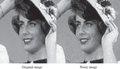
FIGURE 4.1
Original image on the left and corrupted version on the right.

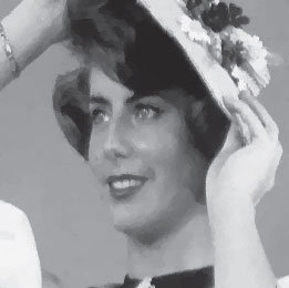
FIGURE 4.2
Denoised image by minimizing DTV with a separable quadratic term.

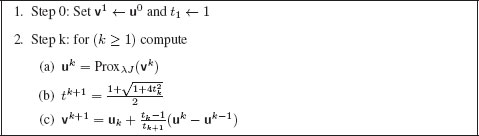
FIGURE 4.3
Algorithm for fast proximal iterations.

This operator is computed exactly by the approach described in this chapter. The general proximal forward–backward iteration [5, 6, 28] takes the following form

$u^{n+1}={\text{Prox}}_{\text{λ}J}\left(u^n-\frac{1}{L}\nabla F\left(u^n\right)\right)$

(4.23)

with L = |∇F|_∞, and this scheme converges toward a solution of F + λJ, provided such a solution does exist. We illustrate this approach with $F\left(u\right)=\frac{1}{2}{\Vert Au-f\Vert }^2$ for image restoration of blurred and noisy images. We consider a blurring operator A that corresponds to a uniform kernel of size 7 × 7. The original image of Figure 4.1 is blurred using this kernel and then corrupted by an additive Gaussian noise of standard variation σ = 3 and null mean to yield to the corrupted image depicted in Figure 4.4 (left). The reconstructed image obtained by iterating the splitting method is depicted in Figure 4.4 (right).

The speed of the proximal splitting algorithm can be improved using acceleration techniques [28, 29, 30]. Compared to the standard proximal iterations, the fast iterates are computed using particular linear combinations of two iterative sequences. Such an algorithm is presented in Figure 4.3. To show the improvement of such an approach we depict in Figure 4.5 the squared distance of the current estimate from the global minimizer (estimated as the solution obtained 1200 iterations) for both the standard and the fast proximal splitting in function of the iterations.

Finally, note that the inversion of A* A could also be performed using Douglas-Rachford splitting [4].

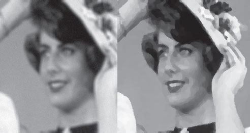
FIGURE 4.4
Blurred and noisy image on the left and reconstructed version on the right.

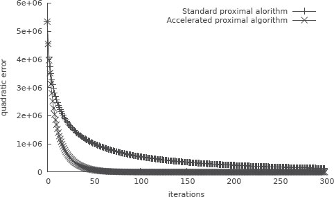
FIGURE 4.5
Plot of the squared distance of the estimate minimizer to the global minimizer with respect to the iterations.

Bibliography

[1]  J. Moreau, “Proximit´e et dualit´e dans un espace hilbertien,” Bulletin de la S.M.F., vol. 93, pp. 273–299, 1965.

[2]  R. Rockafellar and R. Wets, Variational Analysis. Springer-Verlag, Heidelberg, 1998.

[3]  J. Eckstein and D. Bertsekas, “On the Douglas-Rachford splitting method and the proximal point algorithm for maximal monotone operators,” Math. Program., vol. 55, pp. 293–318, 1992.

[4]  P. Lions and B. Mercier, “Splitting algorithms for the sum of two nonlinear operators,” SIAM J. on Numerical Analysis, vol. 16, pp. 964–979, 1992.

[5]  I. Daubechies, M. Defrise, and C. De Mol, “An iterative thresholding algorithm for linear inverse problems with a sparsity constraint,” Comm. Pure Appl. Math., vol. 57, no. 11, pp. 1413–1457, 2004. [Online]. Available: http://dx.doi.org/10.1002/cpa.20042

[6]  P. L. Combettes and V. R. Wajs, “Signal recovery by proximal forward-backward splitting,” Multiscale Model. Simul., vol. 4, no. 4, pp. 1168–1200 (electronic), 2005. [Online]. Available: http://dx.doi.org/10.1137/050626090

[7]  J. C. Picard and H. D. Ratliff, “Minimum cuts and related problems,” Networks, vol. 5, no. 4, pp. 357–370, 1975.

[8]  D. M. Greig, B. T. Porteous, and A. H. Seheult, “Exact maximum a posteriori estimation for binary images,” J. R. Statist. Soc. B, vol. 51, pp. 271–279, 1989.

[9]  G. Gallo, M. D. Grigoriadis, and R. E. Tarjan, “A fast parametric maximum flow algorithm and applications,” SIAM J. Comput., vol. 18, no. 1, pp. 30–55, 1989.

[10]  M. Eisner and D. Severance, “Mathematical techniques for efficient record segmentation in large shared databases,” J. Assoc. Comput. Mach., vol. 23, no. 4, pp. 619–635, 1976.

[11]  D. S. Hochbaum, “An efficient algorithm for image segmentation, Markov random fields and related problems,” J. ACM, vol. 48, no. 4, pp. 686–701 (electronic), 2001.

[12]  Y. Boykov, O. Veksler, and R. Zabih, “Fast approximate energy minimization via graph cuts,” IEEE Trans. Pattern Anal. Mach. Intell., vol. 23, no. 11, pp. 1222–1239, 2001.

[13]  J. Darbon and M. Sigelle, “Image restoration with discrete constrained Total Variation part I: Fast and exact optimization,” J. Math. Imaging Vis., vol. 26, no. 3, pp. 261–276, December 2006.

[14]  ——, “Image restoration with discrete constrained Total Variation part II: Levelable functions, convex priors and non-convex cases,” Journal of Mathematical Imaging and Vision, vol. 26, no. 3, pp. 277–291, December 2006.

[15]  A. Chambolle and J. Darbon, “On total variation minimization and surface evolution using parametric maximum flows,” International Journal of Computer Vision, vol. 84, no. 3, pp. 288–307, 2009.

[16]  J. Darbon, “Global optimization for first order Markov random fields with submodular priors,” Discrete Applied Mathematics, June 2009. [Online]. Available: http://dx.doi.org/10.1016/j.dam.2009.02.026

[17]  A. Chambolle, “Total variation minimization and a class of binary MRF models,” in Energy Minimization Methods in Computer Vision and Pattern Recognition, ser. Lecture Notes in Computer Science, 2005, pp. 136–152.

[18]  H. Ishikawa, “Exact optimization for Markov random fields with convex priors,” IEEE Trans. Pattern Analysis and Machine Intelligence, vol. 25, no. 10, pp. 1333–1336, 2003.

[19]  A. Chambolle, S. Levine, and B. Lucier, “An upwind finite-difference method for total variation–based image smoothing,” SIAM Journal on Imaging Sciences, vol. 4, no. 1, pp. 277–299, 2011. [Online]. Available: http://link.aip.org/link/?SII/4/277/1

[20]  A. Chambolle and T. Pock, “A first-order primal-dual algorithm for convex problems with applications to imaging,” Journal of Mathematical Imaging and Vision, vol. 40, pp. 120–145, 2011. [Online]. Available: http://dx.doi.org/10.1007/s10851-010-0251-1

[21]  F. Bach, “Convex analysis and optimization with submodular functions: a tutorial,” INRIA, Tech. Rep. HAL 00527714, 2010.

[22]  L. Lovász, “Submodular functions and convexity,” in Mathematical programming: the state of the art (Bonn, 1982). Berlin: Springer, 1983, pp. 235–257.

[23]  R. K. Ahuja, T. L. Magnanti, and J. B. Orlin, Network flows. Englewood Cliffs, NJ: Prentice Hall Inc., 1993.

[24]  T. H. Cormen, C. E. Leiserson, R. L. Rivest, and C. Stein, Introduction to Algorithms. The MIT Press, 2001.

[25]  P. Christiano, J. A. Kelner, A. Madry, D. A. Spielman, and S.-H. Teng, “Electrical flows, laplacian systems, and faster approximation of maximum flow in undirected graphs,” CoRR, vol. abs/1010.2921, 2010.

[26]  Y. Boykov and V. Kolmogorov, “An experimental comparison of min-cut/max-flow algorithms for energy minimization in vision,” IEEE Trans. Pattern Analysis and Machine Intelligence, vol. 26, no. 9, pp. 1124–1137, September 2004.

[27]  A. V. Goldberg and R. E. Tarjan, “A new approach to the maximum flow problem,” in STOC ’86: Proc. of the eighteenth annual ACM Symposium on Theory of Computing. New York, NY, USA: ACM Press, 1986, pp. 136–146.

[28]  A. Beck and M. Teboulle, “Fast gradient-based algorithms for constrained total variation image denoising and deblurring problems,” Trans. Img. Proc., vol. 18, pp. 2419–2434, November 2009. [Online]. Available: http://dx.doi.org/10.1109/TIP.2009.2028250

[29]  Y. Nesterov, Introductory Lectures on Convex Optimization: A Basic Course. Kluwer, 2004.

[30]  ——, “Gradient methods for minimizing composite objective function,” Catholic University of Louvain, Tech. Rep. CORE Discussion Paper 2007/76, 2007.

¹In the sequel, c(·, ·) will always denote the residual capacities.