8 Image Denoising with Nonlocal Spectral Graph Wavelets

Effectively modeling the structure of image content is a major theme in image processing. A long and successful tradition of research in image modeling involves applying some transform to the image, and then describing the behavior of the resulting coefficients. In particular, the use of localized, oriented multiscale wavelet transforms and a whole host of variations has been very widespread. A key component of the success of wavelet methods is that images typically contain highly localized features (such as edges) interspersed with relatively smooth regions, resulting in sparse behavior of wavelet coefficients. This type of local regularity in image content is well described by localized wavelets.

Another important type of regularity present in images is self-similarity. Many natural images have similar localized patterns present in spatially distant regions of the image. Self-similarity also occurs in images of man-made structures with repeating features, such as an image containing a brick wall or a building facade with repeated similar windows.

For the problem of restoring images corrupted by noise, it is reasonable that knowledge of which image regions are similar should aid image recovery. Intuitively, averaging over image regions which have similar underlying structure should effect reduction in noise while preserving desired image content. In this work, we describe a novel algorithm for image denoising which seeks to capture nonlocal image regularity while leveraging established transform-based techniques. This is achieved through assuming sparsity of image coefficients under a transform that is constructed to respect the nonlocal structure of the image.

Our approach is based on explicitly describing the image self-similarity by constructing a nonlocal image graph. This is a weighted graph where the vertices are the original image pixels, and the edge weights represent the strength of similarity between image patches. We use a newly described method, the Spectral Graph Wavelet Transform (SGWT), for constructing wavelet transforms on arbitrary weighted graphs [1]. Using the SGWT construction with the nonlocal image graph gives the nonlocal graph wavelet transform. We also explore a class of hybrid weighted graphs which smoothly mix the nonlocal image graph with local connectivity structure. With the SGWT, this produces a hybrid local/nonlocal wavelet transform.

We examine two methods for image denoising, the scaled Laplacian method based on a simple thresholding rule, and a method based on ℓ₁ minimization. The former method is based on modeling the coefficients with a Laplacian distribution, after a simple rescaling needed to account for inhomogeneity in the norms of the nonlocal graph wavelets. With the scaled Laplacian approach, the coefficients are thresholded and the transform is then inverted to give the denoised image. Even though this method operates only a simple operation on each coefficient independently, it gives denoising performance comparable to wavelet methods using much more complicated modeling of the dependencies between coefficients.

The closely related ℓ₁ minimization based algorithm is based on the same underlying nonlocal graph wavelet transform. Rather than treating each coefficient separately, it proceeds by minimizing a single convex functional containing a quadratic data fidelity term and a weighted ℓ₁ prior penalty for the coefficients. We compute the minimum of this functional using an iterative forward-backward splitting procedure. We find the ℓ₁ procedure to give improvements over the scaled Laplacian method in perceived image quality, at the expense of additional computational complexity.

8.1.1 Related Work

The idea of exploiting redundancy present in images due to self-similarity has a long history. A large part of the literature on statistical image modeling concerns describing the strongly related scale-invariance properties of natural images [2, 3, 4]. Quite recently, a number of image processing and denoising methods have sought to exploit image self-similarity through patch-based methods. Of particular relevance for this work is the nonlocal means algorithm for image denoising originally introduced by Buades et al. [5].

Many extensions and variations of the original nonlocal means have been been studied [6, 7, 8]. The basic nonlocal means algorithm proceeds by first measuring the similarity between pairs of noisy image patches by computing the ℓ₂ norms of differences of patches. These are then used to compute weights, such that the weight is high (close to unity) for two similar patches and close to zero for two dissimilar patches. Finally, each noisy pixel is replaced by a weighted average of all other pixels. If a particular patch is highly similar to many other patches in the image, then it will be replaced by a structure that is averaged over a large number of regions, resulting in reduction of noise. The weights used in the nonlocal means algorithm are essentially the same as the edge weights for the nonlocal image graph used in the current work.

Another approach to using patch similarity for denoising is the BM3D collaborative filtering algorithm introduced by Dabov et al. [9]. In this approach, similar patches of the noisy image are stacked vertically to form a 3-D data volume. A separable 3-D transform is applied, then the stacked volumes are denoised by thresholding. The power of this method comes from the interaction of wavelet thresholding with the redundancy presented across the stacks of similar image patches, resulting in an implicit averaging of similar image structure across the patches.

The spectral graph wavelet transform used in this work relies on tools from spectral graph theory, specifically the use of eigenvectors of the graph Laplacian operator. Several authors have employed the graph Laplacian for image processing before. Zhang and Hancock studied image smoothing using the heat kernel corresponding to the graph Laplacian, using a graph whose edge weights depended on the difference of local neighboring windows [10]. Szlam et al. investigated similar heat kernel based smoothing in a more general context, including image denoising examples using nonlocal image graphs more similar to the current work [11]. Peyré used nonlocal graph heat diffusion for denoising, as well as studying thresholding in the basis of eigenvectors of the nonlocal graph Laplacian [12]. Elmoataz et al. [13] studied regularization on arbitrary graph domains, including image processing applications employing nonlocal graphs, with a variational framework employing the p-Laplacian, a nonlinear (for general p) operator reducing to the graph Laplacian for p = 2.

8.2 Spectral Graph Wavelet Transform

The spectral graph wavelet transform (SGWT) is a framework for constructing multiscale wavelet transforms defined on the vertices of an arbitrary finite weighted graph. The SGWT is described in detail in [1]; a brief description of it will be given here.

Weighted graphs provide an extremely flexible way of describing a large number of data domains. For example, vertices in a graph may correspond to individual people in a social network or cities connected by a transportation network of roads. Wavelet transforms on such weighted graph structures thus have the potential for broad applicability to many problems beyond the image denoising application considered in this work. Other authors have introduced methods for wavelet-like structures on graphs. These include vertex-domain methods based on n-hop distance [14], lifting schemes [15], and methods restricted to trees [16]. Gavish et al. have recently described an orthogonal wavelet construction on hierarchical trees, and demonstrated its use for estimating functions on arbitrary graphs by first applying hierarchical clustering of nodes [17]. The above approaches differ from the SGWT primarily in that they are based in the vertex domain, rather than constructed using spectral graph theory. Other constructions using spectral graph theory have been developed, notably the “diffusion wavelets” of Maggioni and Coifman [18]; the primary difference of the SGWT from their approach is in the simplicity of the SGWT construction, and that the SGWT produces an overcomplete wavelet frame rather than an orthogonal basis.

We consider an undirected weighted graph $G$ with N vertices. Any scalar valued function f defined on the vertices of the graph can be associated with a vector in ℝ^N, where the coordinate f_i is the value of f on the i^th vertex. For any real scale parameter t > 0, the SGWT will define the wavelets ψ_t,n ∈ ℝ^N which are centered on each of the vertices n. Key properties of these graph wavelets are that they are zero mean, they are localized around the central vertex n, and they have decreasing support as t decreases.

The SGWT construction is based upon the graph Laplacian operator L, defined as follows. Let W ∈ ℝ^N×N be the symmetric adjacency matrix for $G$ , so that w_i,j ≥ 0 is the weight of the edge between vertices i and j. The degree of vertex i is defined as the sum of the weights of all edges incident to i, i.e., d_i = Σ_j w_i,j. Set the diagonal degree matrix D to have D_i,i = d_i. The graph Laplacian operator is then L = D − W.

The operator L should be viewed as the graph analogue of the standard Laplacian operator −Δ for flat Euclidean domains. In particular, the eigenvectors of L are analogous to the Fourier basis elements e^ik·x, and may be used to define the graph Fourier transform. As L is a real symmetric matrix, it has a complete set of orthonormal eigenvectors χ_ℓ ∈ ℝ^N for ℓ = 0, …, N − 1 with associated real eigenvalues λ_ℓ. We order these in nondecreasing order, so that λ₀ ≤ λ₁ … ≤ λ_N−1. For the graph Laplacian it can be shown the eigenvalues are nonnegative, and that λ₀ = 0. Now for any function f ∈ ℝ^N, the graph Fourier transform is defined by

$\hat{f} (ℓ) = 〈 χ_{ℓ}, f 〉 = \sum_{n} χ_{ℓ}^{*} (n) f (n) .$

(8.1)

We interpret $\hat{f} (ℓ)$ as the ℓ^th graph Fourier coefficient of f. As the χ_ℓ’s are orthonormal, it is straightforward to see that f may be recovered from its Fourier transform by $f = \sum_{ℓ} \hat{f} (ℓ) χ_{ℓ}$ .

The use of the graph Fourier transform for defining the SGWT may be motivated by examining the classical continuous wavelet transform on the real line in the Fourier domain. These wavelets are generated by taking a “mother” wavelet ψ(x), and then applying scaling and translation to obtain the wavelet $ψ_{t, a} = \frac{1}{t} ψ ((x - a) / t)$ [19]. For a given function f, the wavelet coefficients at scale t and location a are then given by inner products, i.e., $W_{f} (t, a) = \int \frac{1}{t} ψ^{*} ((x - a) / t) f (x) d x$ . For fixed scale t, this integral may be rewritten as a convolution evaluated at the point a. Letting ${\bar{ψ}}_{t} (x) = \frac{1}{t} ψ^{*} (- x / t)$ , we see $W_{f} (t, a) = ({\bar{ψ}}_{t} ⋆ f) (a)$ . Now consider taking the Fourier transform over the a variable. On the real line, we may employ the convolution theorem, and this becomes

$\hat{W_{f}} (t, ω) = {\hat{\bar{ψ}}}_{t} (ω) \hat{f} (ω) = {\hat{ψ}}^{*} (t ω) \hat{f} (ω) .$

(8.2)

Thus, the operation of mapping f to its wavelet coefficients W_f(t, a) consists of taking the Fourier transform of f, multiplying by ${\hat{ψ}}^{*} (t ω)$ , and applying the inverse Fourier transform. The key point here is that the operation of scaling by t has been transferred from the original domain to a dilation of the function ${\hat{ψ}}^{*} (t ω)$ in the Fourier domain. This is significant, as a major problem in adapting the classical wavelet transform to graph domains is the inherent difficulty of defining scaling of a function on an irregular graph.

The SGWT operator for fixed scale t is defined in analogy with the previous discussion. Its specific form is fixed by the choice of a nonnegative wavelet kernel g(x), analogous to the Fourier transformed wavelet ${\hat{ψ}}^{*}$ . This kernel g should behave as a band-pass function, specifically we require g(0) = 0 and lim_x→∞ g(x) = 0. For any scale t > 0, the SGWT operator $T_{g}^{t} : ℝ^{N} \to ℝ^{N}$ is defined by $T_{g}^{t} (f) = g (t L) f$ . The result of applying the real-valued function g(t·) to the operator L yields a linear operator, which for symmetric L may be defined by its action on the eigenvectors. Specifically, we have $g (t L) (χ_{ℓ}) \equiv g (t λ_{ℓ}) χ_{ℓ}$ . By linearity, g(tL) applied to arbitrary f ∈ ℝ^N can be expressed in terms of the graph Fourier coefficients, as

$T_{g}^{t} f \equiv g (t L) f = \sum_{ℓ} g (t λ ℓ) \hat{f} (ℓ) χ_{ℓ} .$

(8.3)

Examining this expression, we see that applying $T_{g}^{t}$ to f is equivalent to taking the graph Fourier transform of f, multiplying by the function g(tλ), and then inverting the transform. This is in exact analogy to the Fourier domain description of the classical wavelet transform implied by equation (8.2).

Equation (8.3) defines the N spectral graph wavelet coefficients of f at scale t. We denote these coefficients by W_f (t, n), i.e., so that $W_{f} (t, n) = {(T_{g}^{t} f)}_{n}$ . The wavelets may be recovered by applying this operator to a delta impulse. If we set δ_n ∈ ℝ^N to have value 1 at vertex n and zero’s elsewhere, then the wavelet centered at vertex n is given by $ψ_{t, n} = T_{g}^{t} δ_{n}$ . It is straightforward to verify that this is consistent both with the previous definition of the coefficients and the desire for the coefficients to be generated by inner products, i.e., that $W_{f} (t, n) = 〈 ψ_{t, n}, f 〉$ . In Figure 8.1 we show an example graph with 300 vertices randomly sampled from a smooth manifold, and edges given by connecting all vertices (with unit edge weight) whose distance is below a chosen threshold. We show a single scaling function, and wavelets at two different scales.

The overall stability of the SGWT is improved by including scaling functions to represent the low frequency content of the signal. This is done by introducing a scaling function kernel h, a low-pass function satisfying h(0) > 0, and h(x) → 0 as x → ∞. As with the wavelets, we define the scaling function operator T_h = h(L), scaling functions ϕ_n = T_h δ_n, and the scaling function coefficients of f to be given by T_hf.

The above theory describes the SGWT for continuous scales t. In practice, we will discretize t to a finite number of scales t₁ > … > t_J > 0, as detailed in Section 8.2.3. Once these are fixed, we shall often abuse notation by referring to the wavelet ψ_j,n (or coefficient W_f (j, n)) as shorthand for ψ_{t_j,n} (or W_f (t_j, n)).

We may then consider the overall transform operator T : ℝ^N → ℝ^{(J + 1)N} formed by concatenating the scaling function coefficients and each of the J sets of wavelet coefficients. In ([1], Theorem 5.6) this operator was shown to be a frame, with frame bounds A and B that can be estimated as follows. First define $G (λ) = h^{2} (λ) + \sum_{j = 1}^{J} g^{2} (t_{j} λ)$ . Then for any f ∈ ℝ^N, the inequalities A||f||² ≤ ||Tf||² ≤ B||f||² hold, where A = min_{λ∈[0,λ_N-1]} G(λ), and B = max_{λ∈[0,λ_N−1]} G(λ).

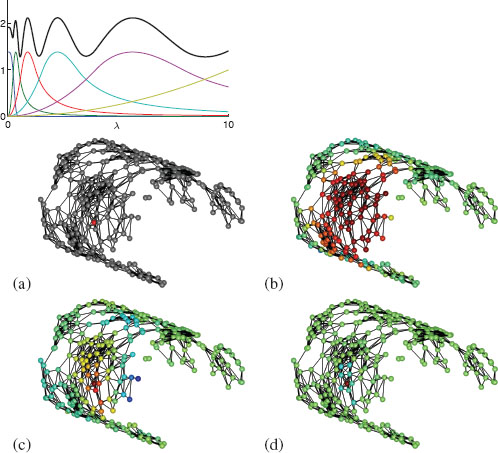
FIGURE 8.1
Left: Scaling function h(λ) (blue curve), wavelet generating kernels g(t_jλ), and sum of squares G (black curve), for J = 5 scales, λ_max = 10, K_1p = 20. Details in Section 8.2.3. Right: Example graph showing specified center vertex (a), scaling function (b) and wavelets at two scales (c,d). Figures adapted from [1].

8.2.1 Fast SGWT via Chebyshev Polynomial Approximation

Direct computation of the SGWT by applying Equation (8.3) requires explicit computation of the entire set of eigenvectors and eigenvalues of L. This approach scales extremely poorly for large graphs, requiring O(N²) memory and O(N³) computational complexity. Direct computation of the SGWT through diagonalizing L is feasible only for graphs with fewer than a few thousand vertices. This limitation would completely destroy the practical applicability of the SGWT for image processing problems, which routinely involve data with hundreds of thousands of dimensions (i.e., number of pixels).

The SGWT coefficients at each scale are given by g(t_j L)f. The fast algorithm avoids the need for diagonalizing L by approximating g(t_jx) by a degree m polynomial p_j(x), where the approximation holds on an interval [0, λ_max] containing the spectrum of L. Once this approximate polynomial is computed, the approximate SGWT coefficients at scale j are given by p_j (L)f.

We compute p_j (x) from Chebyshev polynomial expansion (see, e.g., [20] for overview). The Chebyshev polynomials T_k (x) may be generated from the stable recurrence relation T_k(x) = 2xT_k−1(x) − T_k−2(x) with T₀ = 1 and T₁ = x. For x ∈ [−1,1], they satisfy −1 ≤ T_k (x) ≤ 1, and are a natural basis for approximating functions on the domain [−1,1]. As we require an approximation valid on [0, λ_max], we employ the shifted Chebyshev polynomials ${\bar{T}}_{k} (x) = T_{k} (\frac{x - a}{a})$ with a = λ_max/2. For sufficiently regular g(t_jx), the expansion $g (t_{j} x) = \frac{1}{2} c_{j, 0} + \sum_{k = 1}^{\infty} c_{j, k} {\bar{T}}_{k} (x)$ holds for x ∈ [0, λ_max], with $c_{j, k} = \frac{2}{π} \int_{0}^{π} \cos (k θ) g (t_{j} (a (\cos (θ) + 1))) d θ$ . We compute the c_j,k by numerical integration, and then obtain p_j (x) by truncating the above series to m terms. The wavelet coefficients from the fast SGWT approximation are then given by

${\tilde{W}}_{f} (t_{j}, n) = {(\frac{1}{2} c_{j, 0} f + \sum_{k = 1}^{m} c_{j, k} {\bar{T}}_{k} (L) f)}_{n} .$

(8.4)

We calculate scaling function coefficients similarly with the analogous polynomial approximation for h(x).

Crucially, we may use the Chebyshev recurrence relation to compute the terms ${\bar{T}}_{k} (L) f$ appearing above, accessing L only through matrix-vector multiplication. The shifted Chebyshev polynomials satisfy ${\bar{T}}_{k} (x) = \frac{2}{a} (x - 1) {\bar{T}}_{k - 1} (x) - {\bar{T}}_{k - 2} (x)$ ; it follows that ${\bar{T}}_{k} (L) f = \frac{2}{a} (L - I) ({\bar{T}}_{k - 1} (L) f) - {\bar{T}}_{k - 2} (L) f$ . Viewing each vector ${\bar{T}}_{k} (L) f$ as a single symbol, this implies that ${\bar{T}}_{k} (L) f$ can be computed from the ${\bar{T}}_{k - 1} (L) f$ and ${\bar{T}}_{k - 2} (L) f$ with computational cost dominated by a single matrix-vector multiplication by L. Using sparse matrix representation, the computational cost of applying L is proportional to the number of nonzero edges, making the polynomial approximation algorithm for the SGWT efficient in the important case when the L is sparse.

Further details of the algorithm are given in [1]. In addition, it is shown there that the computational complexity for the fast SGWT is O(m|E| + Nm(J + 1)), where J is the number of wavelet scales, m is the order of the polynomial approximation, and |E| is the number of nonzero edges in the underlying graph $G$ . In particular, for classes of graphs where |E| scales linearly with N, such as graphs of bounded maximal degree, the fast SGWT has computational complexity O(N).

We will require an upper bound λ_max of the largest eigenvalue of L, which may be computed at far lower cost than computing the entire spectrum. We compute a rough estimate of λ_N−1 using Arnoldi iteration, which accesses L only through matrix vector multiplication, then augment this estimate by 1% to get λ_max.

8.2.2 SGWT Inverse

A wide class of signal processing applications, including denoising methods described later in this work, involve manipulating the coefficients of a signal in a certain transform, and later inverting the transform. For the SGWT to be useful for more than simply signal analysis, it is important to be able to recover a signal corresponding to a given set of coefficients.

The SGWT is an overcomplete transform, mapping an input vector f of size N to the N(J + 1) coefficients c = Tf. As is well known, this means that T will have an infinite number of left-inverses B s.t. BTf = f. A natural choice is to use the pseudoinverse T⁺ = (T^TT)⁻¹T^T, which satisfies the minimum-norm property

$T^{+} c = \underset{f \in ℝ^{N}}{\arg \min} ∥ c - T f ∥_{2} .$

For applications which involve manipulation of the wavelet coefficients, it is very likely to need to apply the inverse to a set of coefficients which no longer lie directly in the image of T. In this case, the pseudoinverse corresponds to orthogonal projection onto the image of T, followed by inversion on the image of T.

Given a set of coefficients c, the pseudoinverse will be given by solving the square matrix equation (T^TT)f = T^Tc. This system is too large to invert directly, but may be solved iteratively using conjugate gradients. The computational cost of conjugate gradients is dominated by matrix-vector multiplication by T^TT at each step. As described further in [1], the fast Chebyshev approximation scheme described in Section 8.2.1 may be adapted to compute efficiently the application of either T^T or T^TT. We use conjugate gradients, together with the fast Chebyshev approximation scheme, to compute the SGWT inverse.

The convergence speed of the nonpreconditioned conjugate gradient algorithm is determined by the spectral condition number κ of T^T T, in particular, the error after n steps is bounded by a constant times ${(\frac{\sqrt{κ} - 1}{\sqrt{κ} + 1})}^{n}$ [21]. We note that $κ \leq \frac{A}{B}$ , where A and B are frame bounds for T; the design of the SGWT wavelet and scaling function kernels is influenced by the desire to keep A/B small.

8.2.3 SGWT Design Details

The SGWT framework places very few restrictions on the choice of the wavelet and scaling function kernels. Motivated by simplicity, we choose g to behave as a monic power near the origin, and to have power law decay for large x. In between, we set g to be a cubic spline such that g and g′ are continuous. Specifically, in this work we used

$g (x) = x^{2} ζ_{[0, 1]} (x) + [(x - 1) (x - 2) (x - 3) + 1] ζ_{[1, 2]} (x) + 4 x^{- 2} ζ_{[2, + \infty]} (x),$

(8.5)

where ζ_A(x) is the indicator of A ⊂ ℝ; equal to 1 if x ∈ A and 0 otherwise.

The wavelet scales t_j (with t_j > t_j+1) are selected to be logarithmically equis-paced between the minimum and maximum scales t_J and t₁. These are themselves adapted to the upper bound λ_max of the spectrum of L, described in Section 8.2.1. The placement of the maximum scale t₁ as well as the scaling function kernel h will be determined by the selection of λ_min = λ_max/K_lp, where K_lp is a design parameter of the transform. We then set t₁ so that g(t₁x) has power-law decay for x > λ_min, and set t_J so that g(t_Jx) has monic polynomial behavior for x < λ_max. This is achieved for t₁ = 2/λ_min and t_J = 2/λ_max. We take $h (x) = γ \exp (- {(\frac{x}{0.6 λ_{\min}})}^{4})$ , where γ is set such that h(0) has the same value as the maximum value of g. This set of scaling function and wavelet generating kernels, for parameters λ_max = 10, K_lp = 20, and J = 5, are shown in Figure 8.1.

8.3 Nonlocal Image Graph

The nonlocal image graph is a weighted graph with number of vertices N equal to the number of pixels in the original image. This association assumes some labeling of the two-dimensional pixels, they may for example be labeled in raster-scan order. We will define the edge weights so that the weights will lie between 0 and 1, and will provide a measure of the similarity between image patches.

The number of pixels N for any reasonable sized image will be so large that we cannot reasonably expect to explicitly diagonalize the corresponding graph Laplacian. As we wish to use the SGWT defined on the nonlocal graph, we must produce a graph which is sparse enough to be handled by the fast Chebyshev polynomial approximation scheme.

Given a patch radius K, we let p_i ∈ ℝ^(2K+1)² be the (2K + 1) × (2K + 1) square patch of pixels centered on pixel i. For pixels within distance K of the image boundary, patches may be defined by extending the image outside of its original boundary by reflection. Set d_i,j = ||p_i − p_j|| to be the norm of the differences of patches. Following the weighting used in much of the NL-means literature, we set the edge weights for the (unsparsified) nonlocal image graph to be $w_{i, j} = \exp (- d_{i . j}^{2} / 2 σ_{p}^{2})$ .

In order to sparsify the adjacency matrix of our nonlocal graph, we employ a procedure bounding the degree of each graph vertex, rather than thresholding the values w_i,j to some fixed threshold. In particular, this limits the creation of disconnected vertex clusters. The adjacency matrix W^nl of this sparsified nonlocal image graph is simply obtained by keeping the edges corresponding to the M nearest neighbors (in the patch domain) to each node (excluding self connection). For each node i, we denote the index set of these M nearest nodes $N (i)$ . W^nl is then obtained by symmetrizing the edge connections, that is,

$W_{i, j}^{nl} = {\begin{array}{l} w_{i, j} if i \in N (j) or j \in N (i) \\ 0 otherwise . \end{array}$

After this procedure, each vertex of W^nl will have at least M nonzero edges incident to it, and the total number of nonzero edges will be upper bounded by 2NM. Note that due to the symmetrization of the matrix, it is possible for vertices to have more than M incident nonzero edges.

For convenience in the sequel, we denote by $D (i)$ the ordered set of M patch distances ${d_{i, j} for j \in N (i)}$ . As the function $\exp (- \frac{{(\cdot)}^{2}}{2 σ_{p}^{2}})$ determining w_i,j from d_i,j is decreasing, the elements of $D (i)$ consist of the M smallest patch distances from the patch at vertex i. Note that the sets $N (i)$ and $D (i)$ do not depend on σ_p.

The parameter σ_p is fixed by specifying the desired mean of all of the nonzero elements of W^nl. Given a target mean μ_NL ∈ (0,1), σ_p is set so that

$\frac{1}{| {W_{i, j}^{nl} : W_{i, j}^{nl} \neq 0} |} (\sum_{i, j} W_{i, j}^{nl}) = μ_{NL} .$

We chose to determine σ_p this way, rather than simply fixing a numerical value for it, in order to allow automatic selection of an appropriate σ_p as the input image and other parameters are changed (such as the patch size K). In practice, the value μ_NL = 0.75 gives good results.

8.3.1 Acceleration of Computation with Weeds

Naive computation of the sets $N (i)$ and $\begin{array}{l} D (i) \end{array}$ could be done simply by looping over i, computing the entire set of patch distances d_i,j, sorting them, and retaining the smallest M. This is computationally intensive. In this section we describe an accelerated algorithm for more efficiently computing these sets. We note that a number of other authors have explored various strategies for reducing the computational cost of the closely related nonlocal means filter. Representative approaches include dimensionality reduction of raw patches via PCA [22], and structured organization of patches into a cluster tree [23].

Our “seeds acceleration” algorithm proceeds by exploiting the geometry of the patch space ℝ^(2K+1)² to get lower bounds on distances between patches. These lower bounds will depend on the selection of a set of seed patches to which all distances will be computed. By using the lower bounds to show on the fly that certain patch distances will not appear amongst the M smallest, we will suppress the need to compute them.

Let $S = {s_{1}, \dots, s_{F}}$ be a set of F seeds, with each s_k ∈ ℝ^(2K+1)². We first compute and store the NF values ξ_i,k = ||p_i − s_k||. We then employ the triangle inequality, which shows ||p_i − s_k|| ≤ ||p_i − p_j|| + ||p_j − s_k||, and ||p_j − s_k|| ≤ ||p_j − p_i| + ||p_i − s_k||. These in turn imply

$| (∥ p_{i} - s_{k} ∥ - ∥ p_{j} - s_{k} ∥) | \leq ∥ p_{i} - p_{j} ∥ \equiv d_{i, j} .$

Using this inequality for all k ≤ J shows

$\max_{k} (| ξ_{i, k} - ξ_{j, k} |) \leq d_{i, j} .$

Denote this quantity ${\bar{d}}_{i, j} = \max_{k} (| ξ_{i, k} - ξ_{j, k} |)$ . Computing ${\bar{d}}_{i, j}$ for fixed i,j is very fast (complexity O(F)) as it requires no floating point operations other than absolute value and comparison. Crucially, it is significantly faster than directly computing d_i,j.

We now consider computation of all of the index and distance sets $N (i)$ and $\begin{array}{l} D (i) \end{array}$ . The naive algorithm without using seeds would be Algorithm 1 in Table 8.1. This is wasteful, though, as the entire list L is sorted even though only the M smallest elements are needed. Instead, we can only keep track of the smallest M elements while looping through j. This can be done efficiently using a heap data structure. We are now in a position to use seeds to prune unnecessary computation. If the computed lower bound ${\bar{d}}_{i, j}$ is large enough to ensure that d_i,j exceeds the current heap maximum, then computation of d_i,j may be safely skipped. This yields the accelerated Algorithm 2 in Table 8.1.

We note that as the speedup of the seeds acceleration algorithm is derived from skipping computation of values of d_i,j for j that cannot possibly be among the M smallest, it is not an approximate algorithm. In particular, it will produce exactly the same edge and distance sets as the naive algorithm (unless there are ties in the distances, which may be broken differently).

The performance of the accelerated algorithm is highly dependent on the selection of the seed points s_k. For any patch p_i, the lower bounds (8.6) on d_i,j given by seed s_k will be more informative the closer s_k is to p_i. This implies that a set of seed points will be good if the seeds are near as many patches as possible. On the other hand, if two seeds are close to each other, the information they provide in their lower bounds is redundant. This implies the contrasting criterion that the seeds should be far from each other.

Motivated by these two considerations, we introduce a maxmin heuristic for selecting seed points. This heuristic is an example of the “farthest point” strategy developed previously in the context of progressive image sampling by Eldar [24], and also applied by Peyré et al. in the context of efficient computation of geodesic distances[25]. We select the first seed s₁ to be the patch corresponding to the very middle of the image. We then compute and store the N values ξ_i,1 = ||p_i − s₁||. The next seed s₂ is picked as the point furthest from s₁, i.e., s₂ = arg max_i ξ_{i, 1}. At each successive step, the k + 1^th seed is picked to be the point maximizing the distance to the set {s₁, s₂, …, s_k}, i.e.,

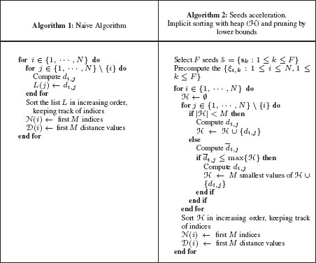
TABLE 8.1
Naive and seeds accelerated algorithms

$s_{k + 1} = \underset{i}{\arg \max} (\min_{k^{'} \leq k} ξ_{i, k^{'}}) .$

This procedure is iterated until all F seeds are computed. Note that the precomputed distances ξ_i,k are produced during the execution of this heuristic.

We have found the performance of the seed acceleration algorithm using seeds computed with the above maxmin heuristic to be slightly better than using the same number of randomly selected seeds. Even using randomly selected seeds, however, provides a marked improvement over the naive algorithm.

The performance of the seeds acceleration can be quantified by the ratio ρ of patch distances d_i,j computed by the accelerated algorithm divided by the number of patch distances computed by the naive algorithm. Alternatively, one may directly

examine the reduction in run time. The overall run time will not be reduced as much as the number of patch distance computations, reflecting the additional overhead of computing the lower bounds ${\bar{d}}_{i, j}$ . Given ρ, a quick computational complexity estimation provides that Algorithm 2 runs in O(NM(2K + 1)² + (N − M)NF + ρ (N − M)N(2K + 1)²). Considering that the proportionality constant are the same in Algorithms 1 and 2, the ratio of computational time is about $ρ + \frac{F}{{(2 K + 1)}^{2}} + \frac{M}{N} .$ Table 8.2 approximately follows this rough estimation.

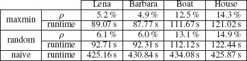
TABLE 8.2
Performance of seeds acceleration algorithm, averaged over 3 trials for K = 5 and M = 10. Runtimes (in seconds) were measured on a parallel implementation using 4 Intel Xeon 2.0 GHz cpu cores.

In practice, on 256 × 256 clean test images with patch radius K = 5, the seeds acceleration algorithm using 15 seeds allows reduction of run time by a factor of 3–8 compared to the naive algorithm for computing the sparsified adjacency matrix, as shown in Table 8.2. We note that the performance improvement is very dependent on the structure of the input image. In particular, when testing on images of random noise, computation time is not reduced at all! This makes sense as the lower bounds are useful only if seeds are near where “most” of the image patches are, for random images the patches are too distributed.

8.4 Hybrid Local/Nonlocal Image Graph

As the spectral graph wavelet transform is parametrized by the underlying weighted graph, great flexibility is available for influencing the wavelets by choosing the design of the graph. While much of the emphasis of this work is on construction of the nonlocal image graph, one may also construct local graph wavelets simply by using a connectivity graph that includes only local connections vertices. Given both the nonlocal adjacency W^nl and a local adjacency W^loc, we may form a hybrid local/nonlocal graph by convex combination, e.g., W^hyb(λ) = λW^loc + (1 − λ)W^nl. Here λ smoothly parametrizes the degree of locality present in the graph, so that at λ = 0 the graph is purely nonlocal, while at λ = 1 it is purely local. The structure of the SGWT makes it extremely easy to explore the effects of such a hybrid connectivity. As long as both the local and nonlocal adjacencies are sufficiently sparse to allow the fast Chebyshev transform to work efficiently, no other changes need be made to any other parts of the SGWT machinery.

In the hybrid graph, the strength of connection between two locations depends both on the similarity of the image content of the two regions and the similarity of the coordinates defining the two locations. This concept is similar in spirit to the “semi-local processing” conditions as described in [12, 23], where image patches are “lifted” to an augmented patch including both the patch center coordinates and image intensity data, before computing patch distance measures. The concept of splitting graph connections into local and nonlocal edge sets is related to the slow/fast patch graph model studied in [26]. Finally, computing filter weights incorporating both domain and range similarity underlies the older bilateral filtering approach [27].

8.4.1 Oriented Local Connectivity

For image processing applications, oriented wavelet filters are generally more effective than spatially isotropic filters, as much of the significant content in images is highly oriented, such as edges. This observation motivates the design of a local adjacency graph that would give oriented filters when used with the SGWT. The standard 4-point local connectivity, with equal edge weights in all directions, gives rise to spectral graph wavelets which are isotropic, and thus unlikely to be highly efficient as a sparsity basis.

We will generate oriented local graph wavelets by choosing a local connectivity which is itself oriented. The design of these oriented local connectivities will be determined by requiring that the associated graph Laplacian approximate a continuous oriented second derivative operator.

We describe the target continuous operator in terms of both a dominant orientation parameter θ, and a second parameter δ ∈ [0,1] specifying the degree of anisotropy, or “orientedness”. For any angle θ, let the perfectly oriented second derivative in the θ direction be $D_{θ}^{2}$ , so that $(D_{θ}^{2} f) (x, y) \equiv \frac{d^{2}}{d ϵ^{2}} f (x + ϵ \cos θ, y + ϵ \sin θ) |_{ϵ = 0}$ for any (x,y) in the plane. For any δ < 1, the target operator D(θ, δ) will include some fraction of the second derivative in the perpendicular direction. Specifically, we define

$D (θ, δ) = \frac{1 + δ}{2} D_{θ}^{2} + \frac{1 - δ}{2} D_{θ + π / 2}^{2} .$

This operator can be expressed in terms of partial derivatives in the standard coordinate directions, as

$D (θ, δ) f = \frac{1}{2} (1 + δ \cos 2 θ) f_{x x} + (δ \sin 2 θ) f_{x y} + \frac{1}{2} (1 - δ \cos 2 θ) f_{y y} .$

(8.7)

We choose the local connectivity $W_{θ, δ}^{loc}$ to be the 8-point connectivity with weights such that the graph Laplacian approximates D(θ, δ). The local connectivity will be completely specified by the values of the weights of any vertex to its 8 nearest neighbors. For convenience, these may be labeled u₁, u₂, …, u₈, as shown in Figure 8.2 (a). As we are considering undirected graphs, we must have equality of edge weights for edges in opposite directions, e.g., u₁ = u₈, u₂ = u₇, u₃ = u₆, u₄ = u₅. We may consider the first four weights as components of the vector u ∈ ℝ⁴.

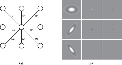
FIGURE 8.2
(a) 8-nearest-neighbor connectivity. The complete graph is produced by reproducing these edges across the entire image. (b) Spectral graph wavelets computed using local oriented adjacencies $W_{θ, δ}^{loc}$ . Shown are scaling functions and wavelets from selected scales for transform with J = 20 wavelet scales, S = 3 orientations, using δ = 0.44. Top row, θ = 0, middle row, θ = π/3, bottom row, θ = 2π/3. Left column, scaling function; middle column, j = 10, right column, j = 20.

We match the discrete graph Laplacian implied by the choice of u to the continuous operator D(θ, δ) by looking at the local Taylor expansion. We now consider f to be a continuous function sampled on the image pixel lattice. Let f_i for 0 ≤ i ≤ 8 denote the value of f at the vertices shown in Figure 8.2, and let x_i and y_i be the integer offsets for vertex i, i.e., (x₁,y₁) = (−1,1), (x₂, y₂) = (0,1), etc. If Δ is the grid spacing, the second order Taylor expansion shows

$f_{i} - f_{0} = Δ (x_{i} f_{x} + y_{i} f_{y}) + \frac{1}{2} Δ^{2} (x_{i}^{2} f_{x x} + 2 x_{i} y_{i} f_{x y} + y_{i}^{2} f_{y y}) + o (Δ^{3}) .$

By above, applying the graph Laplacian to f at the center vertex gives

$\sum_{i} u_{i} (f_{i} - f_{0}) = Δ^{2} (f_{x x} \sum_{i} \frac{1}{2} u_{i} x_{i}^{2} + f_{x y} \sum_{i} u_{i} x_{i} y_{i} + f_{y y} \sum_{i} \frac{1}{2} u_{i} y_{i}^{2}) + o (Δ^{3}) .$

(8.8)

We assume unit grid spacing, i.e., Δ = 1. Equating coefficients of f_xx, f_xy and f_yy in (8.7) and (8.8) yields

${\begin{array}{l} u_{1} + u_{3} + u_{4} & = \frac{1}{2} (1 + δ \cos 2 θ) \\ - u_{1} + u_{3} & = \frac{1}{2} δ \sin 2 θ \\ u_{1} + u_{2} + u_{3} & = \frac{1}{2} (1 - δ \cos 2 θ) \end{array} \Leftrightarrow M u = v (θ, δ),$

(8.9)

where we set $M = (- \begin{matrix} 1 & 0 & 1 & 1 \\ 1 & 0 & 1 & 0 \\ 1 & 1 & 1 & 0 \end{matrix})$ and $v = {(1 / 2, 0, 1 / 2)}^{T} + \frac{δ}{2} {(\cos θ / 2, \sin θ / 2, - \cos θ / 2)}^{T}$ . This is an underdetermined linear system for the four free components of u, which will have an infinite number of solutions for any v(θ, δ). A natural choice for ensuring a unique u is to select the solution with the smallest ℓ₂ norm. Unfortunately, this may produce a solution with negative values for the graph weights, which we require to be nonnegative. Including these two considerations yields a convex optimization program for u :

$u^{*} (θ, δ) = \underset{u}{\arg \min} ∥ u ∥^{2} subject to M u = v (θ, δ), and u_{i} \geq 0.$

(8.10)

For δ close to 1, the program (8.10) fails to be feasible for angles θ away from aligned with the coordinate axes. We have observed through numerical simulation that the program is feasible for all θ whenever $δ < \tilde{δ} \approx 0.44.$ Note that taking δ above $\tilde{δ}$ may still be possible for a specific set of θ values. We solve the program (8.10) numerically using the MATLAB cvx toolbox [28]. Using these values of u(θ, δ) to construct the weighted graph for the entire image yields the local connectivity $W_{θ, δ}^{loc}$ .

For completeness, we show several images of the spectral graph wavelets computed using $W_{θ, δ}^{loc}$ in Figure 8.2(b). The important point of these local oriented wavelets is not necessarily that we expect them to be highly effective for image representation on their own, but rather that they allow the introduction of oriented filter character in a manner compatible with the SGWT construction.

8.4.2 Unions of Hybrid Local/Non-Local SGWT Frames

The SGWT generates a frame of wavelets and scaling functions from a single adjacency matrix. Using a hybrid adjacency with an oriented local connectivity would give a single frame where all of the wavelets had the same directionality. Using such a frame for image restoration tasks is likely to introduce a bias toward orientations in this specific direction. We would prefer a wavelet transform that samples orientations uniformly on [0,π]. A straightforward way to do this is to form the union of multiple SGWT frames corresponding to hybrid adjacencies with uniformly sampled orientations. Let $T^{θ, δ} : ℝ^{N} \to ℝ^{N (J + 1)}$ be the SGWT operator generated using the hybrid adjacency matrix $W_{θ, δ}^{hyb} \equiv λ W_{θ, δ}^{loc} + (1 - λ) W^{nl}$ . Denote by S the number of orientation directions to sample, and set $θ_{k} = \frac{(k - 1) π}{S}$ for 1 ≤ k ≤ S. We then define the overall wavelet transform operator $T : ℝ^{N} \to ℝ^{N S (J + 1)}$ by $T f = {({(T^{^{θ_{1}, δ}} f)}^{T}, {(T^{θ_{2}, δ} f)}^{T}, \dots, {(T^{θ_{S}, δ} f)}^{T})}^{T}$ .

While in principle separate scaling function and wavelet kernels h and g could be used for the separate component SGWT frames, we use the same kernels as well as the same sampled scales t_j for each of the S subframes. As the selection of scales is determined by the spectrum of the graph Laplacian (as described in Section 8.2), choosing the scales uniformly only makes sense if the maximal eigenvalues of the S graph Laplacians formed from each of the $W_{θ_{k}, δ}^{hyb}$ are similar. In practice, we find this to be the case. The oriented local graph Laplacians are approximations of continuous second derivative operators D(θ, δ) which are related to each other by rotation, and should thus have exactly the same spectra. Intuitively, the fact that the maximal eigenvectors of the hybrid Laplacian operators, including the nonlocal component, do not vary strongly with θ reflects a lack of orientation bias in the original image.

The union of frames transformation is itself a frame, where the redundancy is increased by a factor S. If each of the sub-frames satisfy the frame bounds A and B, then the union of frames transformation will have frame bounds SA and SB, and will be S(J + 1) times overcomplete. While highly redundant transforms may be not be appropriate for some signal processing applications such as compression, overcompleteness does not pose a fundamental problem for use of a transform for image denoising. Overcomplete transforms have been widely and successfully used for denoising, e.g., [29, 30, 31, 32], some level of transform redundancy is in fact critical for avoiding problems due to loss of translation invariance [33, 34].

The hybridization with λ may also be described directly with the graph Laplacian operators, i.e. we may write $L_{θ_{k}, δ}^{hyb} = λ L_{θ_{k}, δ}^{loc} + (1 - λ) L^{nl}$ . One issue with this parametrization is that, depending on the parameters of the graph construction, the operator norm of L^nl may be very different in magnitude than that of the $L_{θ_{k}, δ}^{loc}$ ’s. In such a case, taking λ = 0.5 will not really give an equal mixing of local and nonlocal character. For convenience, we introduce the parameter λ′. We wish that the effective nonlocal contribution be proportional to λ′, and the effective local contribution be proportional to 1 − λ′. We enforce this by determining λ so that (1 − λ) ||L^nl|| = (1 − λ′)C, and λ ||L^loc|| = λ′C for some constant C. In the above, we have suppressed the dependence on the angle θ_k for ||L^loc||, as discussed earlier we find there to be little dependence on k and we may just take $∥ L^{loc} ∥ = \max_{k} ∥ L_{θ_{k}, δ}^{loc} ∥$ . Solving the above set of equations gives

$λ = \frac{∥ L^{nl} ∥}{(\frac{1 - λ^{'}}{λ^{'}}) ∥ L^{loc} ∥ + ∥ L^{nl} ∥} .$

Finally, for convenience of notation we note the following. Coefficients of the graph wavelet transforms formed from a single SGWT frame may be indexed by scale parameter j and location index n, while coefficients of the hybrid local/nonlocal wavelet transforms require an additional orientation index k. In the sequel, we will often replace the scale and orientation indices by a single multi-index β associated to one choice of (t_j, θ_k). This allows us to refer to the wavelet ψ_β,n and coefficient x_β,n at (scale and/or orientation) band β, position n, independent of the specific form of the transform.

8.4.3 Image Graph Wavelets

As an illustrative example of what the resulting hybrid local/nonlocal image graph wavelets look like, we display several in Figure 8.3 computed for the well-known “boat” test image. These wavelets were computed using the same parameters as are later used in our denoising applications. A relatively small value of λ′ = 0.15 was used, so they are mostly nonlocal spiced with a small pinch of local character. Note that the wavelets really are nonlocal – this is especially evident with the scaling functions which show support on parts of the image very distant from the wavelet center. It is also evident that the support for both the scaling functions and wavelets consists of image regions that are similar in structure to the center patch. Note for the top row where the center patch is on the ground how the support of the scaling functions are mostly ground and similar blank sky, while for the bottom row the supports consist of regions with strong horizontal structure similar to the patch center. It can also be verified that for increasing j (corresponding to decreasing scale t_j), the wavelets are increasingly localized. For even smaller scales (not pictured), this localization proceeds further.

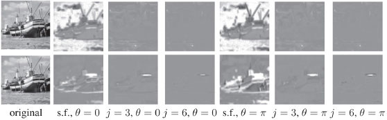
FIGURE 8.3
Images of the graph wavelets with hybrid local/nonlocal adjacency, for the boat image. Shown are scaling functions and wavelets from selected scales for a transform with J = 20 wavelet scales, S = 2 orientations, using δ = 0.5, for two different wavelet centers. Red dots on original image indicate wavelet center locations.

8.5 Scaled Laplacian Model

Coefficients of natural signals in common localized bases (e.g., (bi)orthogonal wavelets, wavelet frames, steerable wavelets, curvelets, …) typically exhibit sparse behavior. This has commonly been modeled by using peaked, heavy-tailed distributions as prior models for coefficients. A canonical example of this is the Laplacian distribution $p (x) = \frac{1}{2 s} \exp (\frac{- | x |}{s})$ . Laplacian models have been very commonly used in the literature to describe the marginal statistics of wavelet coefficients of images, e.g., [35, 36, 37],

Typically, the parameter s is allowed to depend on the wavelet scale. Including this is necessary to allow the variance of the signal coefficients to depend on scale. This effect arises from the power spectral properties of the original image signal (typically showing larger power at low frequencies). It may also arise from normalization of the wavelets themselves, as for many overcomplete wavelet transforms, the norms of the wavelets may depend on the wavelet scale.

Unlike classical wavelet transforms which are translation invariant at each scale (i.e., all wavelets at a particular subband are translates of a single waveform), the spectral graph wavelets centered at different vertices, for a particular wavelet scale t, do not all have the same norm. As the coefficients $c_{β, n} = 〈 ψ_{β, n}, f 〉$ are linear in the norm of each wavelet, it is problematic to model the coefficients at one scale with a single Laplacian density. Allowing the Laplacian parameter s to vary independently at each vertex location n would give a model with too many free parameters that we would not be able to fit.

These considerations motivate the scaled Laplacian model, where we model each coefficient as Laplacian with a parameter that is proportional to the wavelet norm. This proportionality constant is allowed to depend on the wavelet band β, giving one free parameter for the model at each wavelet band. The model is

$p_{β, n} (x) = \frac{1}{2 α_{j} σ_{β, n}} \exp (\frac{- | x |}{α_{β} σ_{β, n}}),$

where σ_β,n = ||ψ_β,n|| is the norm of the wavelet at band β and vertex n.

This model implies that at each band, the marginal distribution of the coefficients rescaled by 1/σ_β,n should have a Laplacian distribution. We find these marginal distributions are qualitatively reasonably fit by a Laplacian, as shown in Figure 8.4. For the higher j scales, the rescaled wavelet marginals appear slightly more kurtotic than the Laplacian fit. These may in fact be better modeled by a generalized Gaussian density of the form p(x) ∝ e^{−|x/s|^p} with an exponent p < 1. Employing such a scaled GGD model for p < 1 would lead to different denoising algorithms, but we do not consider this here. We show results for the purely nonlocal graph wavelet transform, but we observe very similar results for the hybrid local/nonlocal transforms.

We note that many authors have constructed statistical image models employing spatially varying statistical parameters, including [31, 37, 38]. In these works, translation-invariant transforms were used, and the motivation for allowing spatial adaptation of the model is directly to explain the nonstationarity of image content. In contrast, in our work the adaptation of the Laplacian model is motivated by the need to account for the fact that the nonlocal graph wavelets are not translation invariant, and have inhomogeneous norms. This inhomogeneity does arise from the nonstationarity of image content, but not straightforwardly.

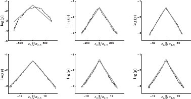
FIGURE 8.4
Log-histograms of rescaled graph wavelet coefficients, from the purely nonlocal transform with 6 wavelet scales, for the clean “boat” image. From top left to bottom right are wavelet scales j = 1 through j = 6. Solid red lines show best Laplacian fit.

8.6 Applications to Image Denoising

As an application of the nonlocal and hybrid graph wavelets, we study the problem of removing noise from natural images. In this work we consider additive Gaussian white noise. We fix our notation as follows. We let x, y, and n denote the (unknown) clean image, noisy image, and noise respectively. This gives the noise model y = x + n, where n is a zero-mean white Gaussian noise with variance $σ_{I}^{2}$ in the pixel domain. Our denoising algorithms are described in wavelet space. Let T be the graph wavelet operator, which will be either the SGWT with nonlocal Laplacian, or a union of SGWT frames for the hybrid local/nonlocal adjacencies described in Section 8.4.2. We will use the notation c, d, and e to refer to the wavelet coefficients of the clean image, noisy image, and noise process, respectively, so that c = Tx, d = Ty, and e = Tn.

8.6.1 Construction of Nonlocal Image Graph from Noisy Image

For a realistic image denoising problem, we cannot measure the true nonlocal image graph as computing it would require the availability of the clean image data. The question of how to estimate the nonlocal image graph is a key concern for our method, as well as for many other works using nonlocal methods, as the effectiveness of the overall nonlocal image denoising procedure is highly dependent on the quality of the estimate underlying nonlocal graph. This presents a chicken-and-egg problem, as denoising the image demands a good quality nonlocal graph, but computing the graph depends on good estimates of the clean image patches.

We have found that directly applying the denoising procedures described in this section using the nonlocal graph computed directly from noisy image patches leads to very poor denoising performance. This is somewhat surprising considering that standard nonlocal means performs well using the same noisy graph. This necessitates the development of some method for robustly estimating the nonlocal graph in the presence of noise. While we have not satisfactorily solved this problem, we still wish to demonstrate the potential of the nonlocal graph wavelet methods for capturing image structure. In this work, we sidestep this issue by using some different image denoising method, dubbed the “predenoiser”, to first estimate the image. We then compute the nonlocal image graph from this “predenoised” image. Once the nonlocal image graph is computed, the predenoised image is discarded and we then proceed purely with our graph wavelet techniques. In this work, we use the Gaussian Scale Mixture model of Portilla et al. [31] to perform the predenoising. As a direction for future research, we may consider jointly estimating the graph weights and the denoised image, through a block relaxation scheme following [39].

While incorporating predenoising yields a highly effective overall denoising algorithm, it introduces some question of how much the performance is depending on the effectiveness of the estimation of the nonlocal graph. To address this, we also examine denoising under the condition where the nonlocal graph is given by an “oracle”, i.e., computed from the original clean image. While this does not result in a true denoising methodology, as it requires access to the original clean image, it does provide an upper bound on the performance of the overall method.

8.6.2 Scaled Laplacian Thresholding

Our first denoising algorithm consists of taking the forward graph wavelet transform, applying a spatially varying soft thresholding operation to the wavelet coefficients, and then inverting the transform. We derive the soft thresholding rule as a Bayesian maximum a posteriori (MAP) estimator, assuming the signal coefficients follow the scaled Laplacian model described in Section 8.5.

Given an input noisy image, we must first estimate the parameters α_β at each wavelet band β. In the wavelet domain, the noise model is d_β,n = c_β,n + e_β,n, where the noise coefficient e_β,n = 〈ψ_β,n, n〉. Assuming signal and noise are independent, we have

$E [d_{β, n}^{2}] = 2 α_{β}^{2} σ_{β, n}^{2} + σ_{I}^{2} σ_{β, n}^{2} \Rightarrow α_{β}^{2} = {(2 \sum_{n} σ_{β, n}^{2})}^{- 1} (\sum_{n} E [d_{β, n}^{2}] - σ_{I}^{2} \sum_{n} σ_{β, n}^{2}) .$

Replacing $\sum_{n} E [d_{β, n}^{2}]$ by the plug-in estimate $\sum_{n} d_{β, n}^{2}$ gives a formula for the estimator ${\tilde{α}}_{β}^{2}$ . For actual data it is possible to obtain a negative value for ${\tilde{α}}_{β}^{2}$ , in this case we set ${\tilde{α}}_{β} = 0$ .

The scaled Laplacian thresholding rule is derived by assuming the independence of wavelet coefficients of both the signal and noise at different spatial locations. In that case, each coefficient d_β,n consists of the sum of the desired signal, a zero mean Laplacian with parameter α_βσ_β,n, and zero mean Gaussian noise with variance $σ_{I}^{2} σ_{β, n}^{2}$ . The MAP estimator for c_β,n in this case is given by soft-thresholding (see, e.g., [40]), i.e.,

$c_{β, n}^{MAP} (d_{β, n}) = \underset{x}{\arg \min} {(d_{β, n} - x)}^{2} + \frac{2 σ_{I}^{2}}{α_{β}} σ_{β, n} | x | = : S_{τ_{β, n}} (d_{β, n}),$

(8.11)

with threshold $τ_{β, n} = \frac{σ_{I}^{2}}{α_{β}} σ_{β, n}$ , where S_τ(y) = (|y| − τ)₊sign(y) with (λ)₊ = max(0, λ). The denoised image is recovered by applying the inverse transform, described in Section 8.2, to the estimated coefficients c^MAP.

The scaled Laplacian model requires knowledge of the norms σ_β,n of the wavelet coefficients. This is somewhat problematic given how the SGWT is computed, as the wavelets are not explicitly formed in memory. Computing these norms by naively applying the SGWT to delta impulses at all image locations would be extremely slow. Instead, we estimate the σ_β,n by computing the variances of the wavelet coefficients of pseudorandom noise. Let e^(k) = Tn^(k), where n^(k) is a sample of zero mean unit white Gaussian noise in the image domain. We estimate σ_β,n by ${\tilde{σ}}_{β, n} = \frac{1}{P} \sum_{k = 1}^{P} {(e_{β, n}^{(k)})}^{2}$ , using P = 100 samples.

8.6.3 Weighted ℓ₁ Minimization

While the scaled Laplacian thresholding may be cleanly motivated by statistical modeling, it is limited in that each wavelet coefficient is processed independently of all the others. As a related alternative denoising algorithm, we develop a variational weighted ℓ₁ minimization procedure which allows for coupling between different wavelet coefficients.

This weighted ℓ₁ functional is obtained from considering the minimization problems from (8.11). Formally, all of these uncoupled minimizations may be written together as

$\underset{c}{\arg \min} \sum_{β, n} {(d_{β, n} - c_{β, n})}^{2} + \sum_{β, n} 2 τ_{β, n} | c_{β, n} | .$

The first term above is the sum of squares of the portion of the wavelet coefficients assigned to the noise process. We arrive at our ℓ₁ program by replacing this term by the sum of squares of the estimated noise in the image domain, where the recovered image is given by T^T c. This yields

$c^{*} \in \underset{c}{\arg \min} ∥ y - T^{T} c ∥^{2} + 2 ∥ c ∥_{τ, 1},$

(8.12)

where T^T c represents the recovered image, ||c||_τ,1 = Σ_β,n τ_β,n|c_β,n| is the τ- weighted ℓ₁-norm of the coefficients c, for the thresholds described previously. The denoised image is then given by x* = T^Tc*.

The objective function in (8.12) is convex in c. This is a BPDN/Lasso problem in Lagrangian form with a synthesis sparsity prior and thus admits a global minimum which can be found by well established minimization techniques like the iterative soft thresholding (IST) [41], the forward-backward (FB) splitting [42], or related approaches [43, 44]. We use the FB method for all of our experiments.

8.6.4 Denoising results

We have performed numerical simulations demonstrating the efficacy of the graph wavelet methods for image denoising. We also explore the change in performance of our denoising methods when the local orientation component of the hybrid local/nonlocal is removed. Our test images were all 256 × 256 pixels in size, with grayscale values ranging between 0 and 255. In all our experiments, reconstructed image qualities have been assessed by the peak signal-to-noise ratio, or PSNR, given by 10 log₁₀ 255² N/||x − x*||², where x ∈ ℝ^N and x* ∈ ℝ^N stand for the original and the reconstructed image.

The extreme flexibility of the methods used in this work give rise to a number of parameters for detailing the specifics of both the SGWT and the graph construction. For convenience, we list them here. For all of our denoising examples, we have used the SGWT with J =20 scales, with K_lp = 200 and polynomial order m = 80 for the fast SGWT transform. The nonlocal image graph was constructed using 11 × 11 patches (i.e., patch radius K = 5), M = 10, and μ_NL = 0.75. For the hybrid local/nonlocal graph, we used S = 2 orientation directions, with δ = 0.5, and normalized hybridization parameter λ′ = 0.15. Note that while δ = 0.5 exceeds the upper bound $\tilde{δ}$ ensuring feasibility of (8.10) for all θ, this is not a problem as (8.10) is feasible with δ = 0.5 for the particular (horizontal and vertical) values of θ implied by S = 2.

Results for the Scaled Laplacian thresholding (SL) and weighted ℓ₁ minimization (ℓ₁-min) algorithms on four standard test images are shown in Table (8.3). Three different levels of noise were tested, with standard deviation σ = 20, 40, and 80. The variants using the oracle to compute the nonlocal graph, as well as variants not using predenoising (i.e., computing the nonlocal graph directly from the noisy image) are also shown. We include comparison against the 8-band GSM used for predenoising, as well as the result of nonlocal means applied using the same nonlocal graph used in the SL and ℓ₁ -min cases. We also compare against the BM3D method [9], which currently defines the state-of-the art for denoising PSNR performance.

We first note that the PSNR performance of both the SL and ℓ₁-min methods are competitive with the 8-band GSM, providing higher performance in a few cases, but typically within 0.2 dB, while the denoising performance of the BM3D method is consistently higher. While the similarity in denoising performance may seem to suggest that the graph wavelet methods are simply reproducing the predenoised image, the results presented really do represent a distinct methodology. This can be seen by examining images of the results, in particular, the visual quality of the GSM predenoiser and the ℓ₁-min method are different. In Figure 8.5, carefully comparing images (c) and (e) shows the presence of unsightly ripple artifacts in the GSM image that are smooth in the ℓ₁-min image, such as near the table edges.

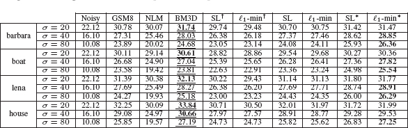
TABLE 8.3
Performance of proposed denoising algorithm and variants (reported by PSNR for 4 standard 256 × 256 test images). In above, GSM8: 8-band GSM method of Portilla et al., used for predenoising; NLM: nonlocal means using same weights as SL and ℓ₁- min; BM3D: Block-matching 3D filtering of Dabov et al.; SL^† and ℓ₁ -min^†: variants of SL and ℓ₁-min where nonlocal graph computed without predenoising; SL: Scaled Laplacian thresholding; ℓ₁-min: weighted ℓ₁ minimization; SL* and ℓ₁-min*: oracle variants. In bold, the highest PSNR per row. Underlined, the best PSNR amongst the non-oracle methods.

Clearly, the good performance of the graph wavelet methods does depend on calculating a good estimate of the nonlocal graph. As shown in Table 8.3, the SL and ℓ₁-min methods calculated using the nonlocal graph computed directly from the noisy image show poorer performance, typically losing over 1dB. In contrast, the oracle methods which use the perfect nonlocal graph show extremely good performance. This is especially noticeable for the high noise (σ = 80) case, exceeding the GSM method by more that 2 dB.

While the PSNR performance of the SL and ℓ₁ -min methods using predenoising are very similar, their visual qualities are different. The SL method results seem oversmoothed compared to the ℓ₁-min results, which preserve sharper edges and generally appear to have more high frequency content. Interestingly, the PSNR of the ℓ₁-min method is consistently better than SL for the oracle case, indicating that the ℓ₁-min method is more sensitive to the quality of the nonlocal graph. The computational cost of the two methods is shown in Table 8.4. For the SL method, the run-time is dominated by computing the nonlocal graph and the wavelet norms, while for the ℓ₁-min method the FB iteration is the largest part of the overall run-time.

The nonlocal graph used in our methods has weights that are computed the same way as those used in the nonlocal means method for image denoising. As both the nonlocal graph wavelet methods and nonlocal means can be described using the same underlying graph structure, it is interesting to compare against the results of nonlocal means computed with the same nonlocal graph. Given the adjacency matrix W, the nonlocal means proceeds by replacing each pixel of the noisy image by the weighted average of its graph neighbors. Recall that W is defined with zeros on the diagonal; the nonlocal means denoising result is

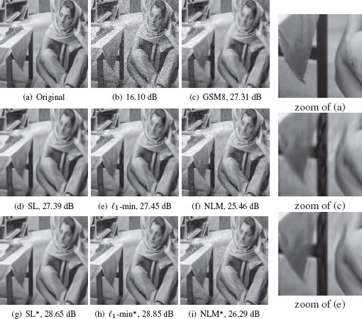
FIGURE 8.5
Denoising results. NonlocalmMeans* is for nonlocal means with oracle graph.

$x_{NLM}^{*} (j) = \frac{y (j) + \sum_{i} w_{i, j} y (i)}{1 + \sum_{i} w_{i, j}} .$

(8.13)

We show the result of this nonlocal means in Figure 8.5, and note that the performance of the graph wavelet methods is much better. It should be noted that the nonlocal means results shown here are not the best results that can be obtained with the nonlocal means algorithm. The graph construction here has been optimized to give good results for the graph wavelet methods. We have observed that different choices for the graph sparsification and μ_NL can improve the nonlocal means performance. However, the dramatic difference in performance when using the same graph emphasizes that the graph wavelet methods are really doing something beyond simple nonlocal means.

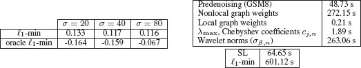
TABLE 8.4
Left: PSNR(λ′ = 0.15) - PSNR(λ′ = 0), averaged over 16 test images under different noise conditions. Right: CPU time for different stages of denoising, averaged over same four test images as in Table 8.3. Times for all steps in left column must be incurred for both SL and ℓ₁-min methods, right column gives the additional CPU time required for either SL or ℓ₁-min. Run-time measured with a MATLAB implementation running on one core of a 2.66 GHz Intel Xeon processor.

In order to assess the usefulness of introducing orientation through the local/nonlocal hybridization described in Section 8.4, we have studied the change in performance when the local oriented adjacency is removed (i.e., setting λ′ = 0). Results averaged over a larger set of 16 test images are shown in Table 8.4. Including the oriented local component provides a moderate improvement on average when the nonlocal graph is computed via predenoising. Interestingly, including the local component actually degrades performance when the oracle graph is used. This suggests that the usefulness of the local component is to provide some regularization of the imperfectly estimated nonlocal graph. For the oracle case, as the nonlocal graph is perfectly estimated, the local component is not needed.

8.7 Conclusions

We have introduced a novel image model based on describing the wavelet coefficients under a new nonlocal image graph wavelet transform. The underlying nonlocal image graph has vertices associated with the image pixels, and edge weights which measure the similarity of different image patches. We constructed an overcomplete frame of wavelets on this graph using the spectral graph wavelet transform, and showed that the nonlocal graph wavelet coefficients of images are well modeled by a scaled Laplacian probability model. We also detailed a way for building local oriented wavelets with the spectral graph wavelet transform, enabling the construction of hybrid local/nonlocal graph wavelets.

As a demonstration of the power of the image graph wavelets, we have developed two related methods for image denoising based on the scaled Laplacian model. A straightforward Bayesian MAP inference in the wavelet domain leads to the scaled Laplacian thresholding method. The second weighted ℓ₁ method uses the scaled Laplacian prior as part of a global convex objective function, leading to improved recovery of higher frequency image features.

There are many opportunities for future work using the nonlocal image graph wavelets. At present, we are actively investigating the use of nonlocal image graph wavelets for other image processing problems. Both image deconvolution and image super-resolution problems may be cast in a convex variational framework as the ℓ₁-min method. An additional important question is how to improve the estimation of the nonlocal graph, hopefully to avoid the somewhat awkward use of the predenoising method.

8.8 Acknowledgments

DH is funded by the US DoD TATRC Research Grant # W81XWH-09-2-0114.

LJ is funded by the Belgian Science Policy (Return Grant, BELSPO, Belgian Interuniversity Attraction Pole IAP-VI BCRYPT).

Bibliography

[1] D. K. Hammond, P. Vandergheynst, and R. Gribonval, “Wavelets on graphs via spectral graph theory,” Applied and Computational Harmonic Analysis, vol. 30, pp. 129–150, 2011.

[2] D. L. Ruderman and W. Bialek, “Statistics of natural images: Scaling in the woods,” Physical Review Letters, vol. 73, pp. 814–817, 1994.

[3] D. B. Mumford and B. Gidas, “Stochastic models for generic images,” Quarterly of Applied Mathematics, vol. 59, pp. 85–111, 2001.

[4] A. B. Lee, D. Mumford, and J. Huang, “Occlusion models for natural images: A statistical study of a scale-invariant dead leaves model,” International Journal of Computer Vision, vol. 41, pp. 35–59, 2001.

[5] A. Buades, B. Coll, and J. M. Morel, “A review of image denoising algorithms, with a new one,” Multiscale Modeling & Simulation, vol. 4, pp. 490–530, 2005.

[6] G. Gilboa and S. Osher, “Nonlocal linear image regularization and supervised segmentation,” Multiscale Modeling & Simulation, vol. 6, pp. 595–630, 2007.

[7] A. Buades, B. Coll, and J.-M. Morel, “Nonlocal image and movie denoising,” International Journal of Computer Vision, vol. 76, pp. 123–139, 2008.

[8] L. Pizarro, P. Mrazek, S. Didas, S. Grewenig, and J. Weickert, “Generalised nonlocal image smoothing,” International Journal of Computer Vision, vol. 90, pp. 62–87, 2010.

[9] K. Dabov, A. Foi, V. Katkovnik, and K. Egiazarian, “Image denoising by sparse 3D transformdomain collaborative filtering,” IEEE Transactions on Image Processing, vol. 16, pp. 2080–2095, 2007.

[10] F. Zhang and E. R. Hancock, “Graph spectral image smoothing using the heat kernel,” Pattern Recogn, vol. 41, pp. 3328–3342, 2008.

[11] A. D. Szlam, M. Maggioni, and R. R. Coifman, “Regularization on graphs with function-adapted diffusion processes,” Journal of Machine Learning Research, vol. 9, pp. 1711–1739, 2008.

[12] G. Peyré, “Image processing with nonlocal spectral bases,” Multiscale Modeling & Simulation, vol. 7, pp. 703–730, 2008.

[13] A. Elmoataz, O. Lezoray, and S. Bougleux, “Nonlocal discrete regularization on weighted graphs: A framework for image and manifold processing,” IEEE Transactions on Image Processing, vol. 17, pp. 1047–1060, 2008.

[14] M. Crovella and E. Kolaczyk, “Graph wavelets for spatial traffic analysis,” INFOCOM, pp. 1848–1857, 2003.

[15] M. Jansen, G. P. Nason, and B. W. Silverman, “Multiscale methods for data on graphs and irregular multidimensional situations,” Journal of the Royal Statistical Society: Series B, vol. 71, pp. 97–125, 2009.

[16] A. B. Lee, B. Nadler, and L. Wasserman, “Treelets – an adaptive multi-scale basis for sparse unordered data,” Annals of Applied Statistics, vol. 2, pp. 435–471, 2008.

[17] M. Gavish, B. Nadler, and R. Coifman, “Multiscale wavelets on trees, graphs and high dimensional data: Theory and applications to semi supervised learning,” in International Conference on Machine Learning, 2010.

[18] R. R. Coifman and M. Maggioni, “Diffusion wavelets,” Applied and Computational Harmonic Analysis, vol. 21, pp. 53–94, 2006.

[19] I. Daubechies, Ten Lectures on Wavelets. Society for Industrial and Applied Mathematics, 1992.

[20] G. M. Phillips, Interpolation and Approximation by Polynomials. Springer-Verlag, 2003.

[21] G. Golub and C. V. Loan, Matrix Computations. Johns Hopkins University Press, 1983.

[22] T. Tasdizen, “Principal neighborhood dictionaries for nonlocal means image denoising,” IEEE Transactions on Image Processing, vol. 18, pp. 2649–2660, 2009.

[23] T. Brox, O. Kleinschmidt, and D. Cremers, “Efficient nonlocal means for denoising of textural patterns,” Image Processing, IEEE Transactions on, vol. 17, pp. 1083–1092, 2008.

[24] Y. Eldar, M. Lindenbaum, M. Porat, and Y. Zeevi, “The farthest point strategy for progressive image sampling,” IEEE Transactions on Image Processing, vol. 6, pp. 1305–1315, 1997.

[25] G. Peyré and L. Cohen, “Geodesic remeshing using front propagation,” International Journal of Computer Vision, vol. 69, pp. 145–156, 2006.

[26] K. M. Taylor and F. G. Meyer, “A random walk on image patches,” 2011, arXiv:1107.0414v1 [physics.data-an].

[27] C. Tomasi and R. Manduchi, “Bilateral filtering for gray and color images,” IEEE International Conference on Computer Vision, vol. 0, p. 839, 1998.

[28] M. Grant and S. Boyd, “CVX: Matlab software for disciplined convex programming,” http://cvxr.com/cvx.

[29] I. Selesnick, R. Baraniuk, and N. Kingsbury, “The dual-tree complex wavelet transform,” Signal Processing Magazine, IEEE, vol. 22, pp. 123–151, 2005.

[30] J.-L. Starck, E. Candes, and D. Donoho, “The curvelet transform for image denoising,” IEEE Transactions on Image Processing, vol. 11, pp. 670–684, 2002.

[31] J. Portilla, V. Strela, M. J. Wainwright, and E. P. Simoncelli, “Image denoising using scale mixtures of Gaussians in the wavelet domain,” IEEE Transactions on Image Processing, vol. 12, pp. 1338–1351, 2003.

[32] M. Elad and M. Aharon, “Image denoising via sparse and redundant representations over learned dictionaries,” IEEE Transactions on Image Processing, vol. 15, pp. 3736–3745, 2006.

[33] R. R. Coifman and D. L. Donoho, “Translation invariant de-noising,” in Wavelets and Statistics, A. Antoniadis and G. Oppenheim, Eds. Springer-Verlag, 1995, pp. 125–150.

[34] M. Raphan and E. Simoncelli, “Optimal denoising in redundant representations,” IEEE Transactions on Image Processing, vol. 17, pp. 1342–1352, 2008.

[35] S. Mallat, “A theory for multiresolution signal decomposition: the Wavelet representation,” IEEE Pattern Analysis and Machine Intelligence, vol. 11, 1989.

[36] P. Moulin and J. Liu, “Analysis of multiresolution image denoising schemes using generalized Gaussian and complexity priors,” IEEE Transactions on Information Theory, vol. 45, pp. 909–919, 1999.

[37] H. Rabbani, “Image denoising in steerable pyramid domain based on a local Laplace prior,” Pattern Recognition, vol. 42, pp. 2181–2193, 2009.

[38] S. Lyu and E. Simoncelli, “Modeling multiscale subbands of photographic images with fields of Gaussian scale mixtures,” IEEE Transactions on Pattern Analysis and Machine Intelligence, vol. 31, pp. 693–706, 2009.

[39] G. Peyré, S. Bougleux, and L. Cohen, “Non-local regularization of inverse problems,” in European Conference on Computer Vision (ECCV), 2008, pp. 57–68.

[40] A. Chambolle, R. De Vore, N.-Y. Lee, and B. Lucier, “Nonlinear wavelet image processing: variational problems, compression, and noise removal through wavelet shrinkage,” IEEE Transactions on Image Processing, vol. 7, pp. 319–335, 1998.

[41] I. Daubechies, M. Defrise, and C. D. Mol, “An iterative thresholding algorithm for linear inverse problems with a sparsity constraint,” Communications on Pure and Applied Mathematics, vol. 57, pp. 1413–1457, 2004.

[42] P. Combettes and V. Wajs, “Signal recovery by proximal forward-backward splitting,” Multiscale Model Sim, vol. 4, pp. 1168–1200, 2005.

[43] J. Bioucas-Dias and M. Figueiredo, “A new twist: Two-step iterative shrinkage/thresholding algorithms for image restoration,” Image Processing, IEEE Transactions on, vol. 16, pp. 2992–3004, 2007.

[44] M. Figueiredo, R. Nowak, and S. Wright, “Gradient projection for sparse reconstruction: Application to compressed sensing and other inverse problems,” Selected Topics in Signal Processing, vol. 1, pp. 586–597, 2007.

..................Content has been hidden....................

You can't read the all page of ebook, please click here login for view all page.

Table of Contents for 8 Image Denoising with Nonlocal Spectral Graph Wavelets

Create new playlist

Sign In

Sign Up

Table of Contents for
8 Image Denoising with Nonlocal Spectral Graph Wavelets