12 Graph-Based Dimensionality Reduction

Dimensionality reduction aims at representing high-dimensional data into low-dimensionality space. In order to make sense, the low-dimensional representation, or embedding, has to preserve some well-defined structural properties of data. The general idea is that similar data items should be displayed close to each other, whereas longer distances should separate dissimilar ones. This principle applies to data that can be either sampled from a manifold of the data space or distributed among several clusters. In both cases, one generally agrees that rendering the local struture comes prior to reproducing the global arrangement of data. In practice, the structural properties can be pairwise measurements such as dissimilarities (all kinds of distances) or similarities (decreasing functions of distances). Relative proximities such as rank of sorted distances can be used as well. Within this context, graphs can serve several purposes. For instance, they can model the fact that (dis)similarities are missing or overlooked. Even if all pairwise dissimilarities are available, one can consider that only the shortest ones are meaningful and reflect the local data structure. Graphs corresponding to K-ary neighborhoods or ϵ-balls can be built and utilized to compute the length of shortest paths or commute-time distances associated to random walks.

This chapter reviews some of the most prominent dimensionality reduction methods that rely on graphs. These include several techniques based on geodesic distances, such as Isomap and its variants. Spectral methods involving a graph Laplacian are described as well. More biologically inspired techniques, such as the selforganizing map, identify a topographic mapping between a predefined graph and the data manifold. Illustrative experiments focus on image data (scanned handwritten digits) and results are assessed using rank-based quality criteria.

12.2 Introduction

The interpretation of high-dimensional data remains a difficult task, mainly because human vision is not used to deal with spaces having more than three dimensions. Part of this difficulty stems from the curse of dimensionality, a convenient expression that encompasses all weird and unexpected properties of high-dimensional spaces. Dimensionality reduction (DR) aims at constructing an alternative low-dimensional representation of data, in order to improve readability and interpretability. Of course, this low-dimensional representation must be meaningful and faithful to the genuine data. In practice, the representation must preserve important structural properties of the data set, such as relative proximities, similarities, or dissimilarities. The general idea is that dissimilar data items should be represented far from each other, whereas similar ones should appear close to each other. Dimensionality reduction serves other purposes than just data visualization. For instance, DR can be used in data compression and denoising. It can also preprocess data, with the hope that a simplified representation can accelerate any subsequent processing or improve its outcome.

Linear DR is well known, with techniques such as principal component analysis [1] (PCA) and classical metric multidimensional scaling [2, 3] (MDS). The former tries to preserve the covariances in the low-dimensional space, whereas the latter attempts to reproduce the Gram matrix of pairwise dot products. Nonlinear dimensionality reduction [4] (NLDR) emerged later, with nonlinear variants of multidimensional scaling [5, 6, 7] such as Sammon’s nonlinear mapping [8] (NLM) and curvilinear component analysis [9, 10] (CCA). Most of these methods are based on the preservation of pairwise distances. Research in NLDR is multidisciplinary and follows many approaches, ranging from artificial neural networks [11, 12, 13, 9, 14] to spectral techniques [15, 16, 17, 18, 19, 20, 21]. If linear DR assumes that data are distributed within or near a linear subspace, NLDR necessitates more complex models.

The most generic framework consists in assuming that data are sampled from a smooth manifold. For this reason, modern NLDR is sometimes referred to as manifold learning [22, 20]. Under this hypothesis, one seeks to re-embed the manifold in a space having the lowest possible dimensionality, without modifying its topological properties. In practice, smooth manifolds are difficult to conciliate with the discrete nature of data. In constrast, graph structures have proven to be very useful, and tight connections between NLDR and graph embedding [23, 24, 25] exist.

Another usual hypothesis is to assume that data are sampled from clusters rather than from a manifold. Dimensionality reduction methods that emphasize clusters are often closely related to spectral clustering [26, 27, 28, 29]. In this domain, graphs are very handy as well, with useful tools such as the Laplacian matrix.

This chapter is organized as follows. Section 12.3 introduces the necessary notations and classical methods such as PCA and MDS. Section 12.4 details how graphs can help introducing nonlinearities in the DR methods. Next, Sections 12.5 and 12.6 review some of the major DR methods that perform manifold learning by using either distances (global methods) or similarities (local methods). Section 12.7 deals with graph embedding, another paradigm used in nonlinear dimensionality reduction. Finally, Section 12.8 compares the methods on a few examples, before Section 12.9 that draws the conclusions and sketches some perspectives for the near future.

12.3 Classical methods

Let X = [X_i]_1≤i≤N denotes a multivariate data set, with X_i ∈ ℝ^M. Let Y = [y_i]_1≤i≤N denote its low-dimensional representation, with y_i ∈ ℝ^P and P < M. Dimensionality reduction aims at finding a tranformation $T$ from ℝ^M×N to ℝ^P×N that minimizes the reconstruction error defined by

$E = ∥ X - T^{- 1} (Y) ∥_{2}^{2},$

(12.1)

where Y = $T (X)$ and $∥ U ∥_{2}^{2}$ = Tr(U^TU) = Tr(UU^T) is the Frobenius norm of U. In other words, the encoding-decoding process resulting from the successive application of $T$ and $T^{- 1}$ should produce minimal distortion.

12.3.1 Principal component analysis

The simplest option for $T$ is obviously a linear transformation. In principal component analysis [30, 31, 32, 33, 1], this transformation can be written as $T (X) = V_{P}^{T} (X - u 1^{T})$ , where u is an offset and V_P is an orthogonal matrix ( $(V_{P}^{T} V_{P} = 1)$ ) with P columns. Orthogonality reduces the number of free parameters in V_P and provides the P-dimensional subspace of ℝ^M with a basis of orthonormal vectors. With such a linear transformation, the reconstruction error can be rewritten as

$E (u, V_{P}; X) = ∥ (X - u 1^{T}) - V_{P} V_{P}^{T} (X - u 1^{T}) ∥_{2}^{2}$

(12.2)

$= ∥ (l - V_{P} V_{P}^{T}) (X - u 1^{T}) ∥_{2}^{2}$

(12.3)

$= Tr ({(X - u 1^{T})}^{T} (l - V_{P} V_{P}^{T}) (l - V_{P} V_{P}^{T}) (X - u 1^{T}))$

(12.4)

$= Tr ({(X - u 1^{T})}^{T} (l - V_{P} V_{P}^{T}) (X - u 1^{T})) .$

(12.5)

In order to identify u, we can compute the partial derivative of the reconstruction error with respect to u and equate it with zero. Defining E = X – u1^T, we have

$\frac{\partial E (u, V_{P}; X)}{\partial u} = \frac{\partial Tr (E^{T} (l - V_{P} V_{P}^{T}) E)}{\partial E} \frac{\partial E^{T}}{\partial u} = 2 (l - V_{P} V_{P}^{T}) E 1 = 0$

(12.6)

Assuming that $l - V_{P} V_{P}^{T}$ has full rank, we have (X − u1^T)1^T = 0 and therefore u = X1^T/N. The optimal offset is thus the sample mean of X. Knowing this, we can simplify the transformation into $T (X) = V_{P}^{T} X$ if we assume that X1 = 0. The reconstruction error is then rewritten as

$E (V_{P}; X) = ∥ (l - V_{P} V_{P}^{T}) X ∥_{2}^{2} = Tr (X X^{T}) - Tr (V_{P}^{T} X X^{T} V_{P}),$

(12.7)

where the first term is constant. The second term can be minimized under the constraint $V_{P}^{T} V_{P} = l$ using Lagrange’s technique. The Lagrangian can be written as

$L (V_{P}, ⋀; X) = Tr (V_{P}^{T} X X^{T} V_{P}) + Tr (⋀ (l - V_{P}^{T} V_{P})),$

(12.8)

where ⋀ is the diagonal matrix containing Lagrange’s multipliers. The partial derivative of L(V_P, ⋀; X) with respect to V_P is given by

$\frac{\partial L (V_{P}, \land; X)}{\partial V_{P}} = 2 X X^{T} V_{P} - 2 \land V_{P} .$

(12.9)

After equating the partial derivative with zero and rearranging the terms, we obtain ⋀V_P = XX^TV_P, which turns out to be an eigenproblem. Without loss of generality and because X is centered, the product XX^T can be replaced with the sample covariance C(X) = XX^T/N. The covariance matrix is symmetric and positive semidefinite by construction. Its eigenvalues are therefore larger than or equal to zero. If we write the eigenvalue decomposition as C(X) = V⋀V^T, then the solution of the maximization problem for a given P is provided by the eigenvectors in V that are associated with the P largest eigenvalues. These eigenvectors give the columns of V_P = [v_i]_1≤i≤P. The covariance in the P-dimensional subspace is given by

$C (Y) = Y Y^{T} / N = V_{P}^{T} X X^{T} V_{P} / N = V_{P}^{T} C (X) V_{P} = V_{P}^{T} V_{P} \land V_{P}^{T} V_{P} = \land_{P},$

(12.10)

where ⋀_P denotes the restriction of ⋀ to its first P rows and columns. As the covariance is diagonal in the subspace, this shows that PCA also decorrelates the data set. Matrix V_P is also the solution that minimizes $∥ C (X) - V_{P} \land_{P} V_{P}^{T} ∥_{2}^{2}$ . This shows that minimal reconstruction error is equivalent to variance preservation. If V_P maximizes $Tr (V_{P}^{T} X X^{T} V_{P})$ , then it also trivially maximizes $Tr (X^{T} V_{P} V_{P}^{T} X)$ .

12.3.2 Multidimensional scaling

In the previous section, PCA requires the data set to be available in the form of coordinates in X. In contrast, classical metric multidimensional scaling [2, 3](CMMDS) starts from the Gram matrix, which is defined as G(X) = X^TX and is positive semidefinite by construction. The aim and model of CMMDS are basically the same as those of PCA. The solution remains the same as well, but it is computed differently. To see this, let us use the singular value decomposition of X. It can be written as X = VSU^T, where both U and V are orthogonal matrices and S contains the singular values on its diagonal in descending order of magnitude. The covariance matrix can be rewritten as C(X) = XX^T/N = VSU^TUS^TV^T/N = V(SS^T/N)V^T. The last expression is equivalent to the eigenvalue decomposition of the covariance matrix if we rename the product SS^T/N into ⋀. Similarly, the Gram matrix can be rewritten as G(X) = X^TX = US^TV^TVSU^T = U(S^TS)U^T. The last expression is equivalent to the eigenvalue decomposition of the Gram matrix and shows the tight connection with the eigenvalue decomposition of the covariance matrix. The coordinates in the P-dimensional subspace can be rewritten as $Y = V_{P}^{T} X = V_{P} V S U^{T} = S_{P} U^{T}$ , where S_P is the restriction of S to its P first columns. This shows that the coordinates are given by the P leading eigenvectors of the Gram matrix, scaled by the square root of their associated eigenvalue.

Until here, we have assumed that X is centered in the Gram matrix. If it is not, then we need to compute

$G (X) = {(X - (X 1 / N) 1^{T})}^{T} (X - (X 1 / N) 1^{T}) = (l - 1 1^{T} / N) (X^{T} X) (l - 1 1^{T} / N) .$

(12.11)

This shows that the Gram matrix can be centered as such, without explicitly knowing X. The centering matrix I − 11^T/N is a powerful tool that can also be used if the data set consists of pairwise squared Euclidean distances. In this case, we write

$Δ^{2} (X) = {[∥ x_{i} - x_{j} ∥_{2}^{2}]}_{1 \leq i, j \leq N} = diag (G (X)) 1^{T} - 2 G (X) + 1 diag {(G (X))}^{T},$

(12.12)

where operator diag provides the column vector built from the diagonal entries of its argument. Double centering, namely, multiplying the matrix of squared distances by the centering matrix on both the left and right sides, yields

$(I - 1 1^{T} / N) Δ^{2} (X) (I - 1 1^{T} / N) = - 2 (I - 1 1^{T} / N) G (X) (I - 1 1^{T} / N) .$

(12.13)

This results from

$diag (G (X)) 1^{T} (I - 1 1^{T} / N) = diag (G (X)) 1^{T} - diag (G (X)) 1^{T} 1 1^{T} / N$

(12.14)

$= diag (G (X)) 1^{T} - diag (G (X)) 1^{T}$

(12.15)

$= 0 0^{T}$

(12.16)

and similarly (I − 11^T/N)1 diag(G(X))^T = 00^T. Classical metric MDS is thus a flexible method that can be applied to coordinates, pairwise dot products, or pairwise squared Euclidean distances. For a given P, it can be shown that Y = S_PU^T minimizes a cost function called STRAIN [34] and defined as

$E (Y; X) = ∥ G (X) - G (Y) ∥_{2}^{2} = {\sum_{i, j} (x_{i}^{T} x_{j} - y_{i}^{T} y_{j})}^{2} .$

(12.17)

In other words, CMMDS tries to preserve dot products in the linear subspace.

12.3.3 Nonlinear MDS and Distance Preservation

Given the close relationship between dot products and squared Euclidean distances, one might extend the CMMDS principle to distance preservation. Unfortunately, distance preservation cannot be achieved with spectral decomposition such as in PCA and CMMDS. It requires more generic optimization tools such as gradient descent or ad hoc algorithms. As an advantage, these tools are quite flexible and allow for more freedom in the definition of the cost function to be minimized. This freedom also means that the P-dimensional coordinates are no longer constrained to a linear transformation of those in the M-dimensional space. For instance, one can consider the STRESS function [6] defined as $E (D; Δ) = ∥ Δ (X) - Δ (Y) ∥_{2}^{2}$ . If δ_ij(X) and δ_ij(Y) denote the pairwise distance in the M- and P-dimensional space, respectively, then a more general form of the STRESS is given by

$E (Y; X) = \sum_{i, j} w_{i j} {(δ_{i j} (X) - δ_{i j} (X))}^{2},$

(12.18)

where w_ij controls the weight of each difference of distances in the cost function. These weights can be chosen arbitrarily or can depend on δ_ij and/or d_ij. The emphasis put on the preservation of small distances can be reinforced by defining w_ij = 1/δ_ij, such as in Sammon’s stress function, which is used in his nonlinear mapping (NLM) technique [8]. Another possibility is to define w_ij = f (δ_ij), where f is a nonincreasing positive function. For instance, in curvilinear component analysis (CCA) [10], we have w_ij = H(λ_i − δ_ij), where H is a step function and λ_i a width parameter.

Yet another cost function for MDS is the squared stress, often shortened as SSTRESS [7], whose generic definition is

$E (Y; X) = \sum_{i, j} w_{i j} {(δ_{i j}^{2} (X) - δ_{i j}^{2} (Y))}^{2} .$

(12.19)

As distances are squared, the SSTRESS is actually closer to the STRAIN of CM-MDS.

Various optimization procedures can be used to minimize these cost functions. Gradient descent with a diagonal approximation of the Hessian is used in Sammon’s NLM, whereas CCA relies on a stochastic gradient descent. Yet another technique consists of successive majorizations of the STRESS with convex functions whose minimum can be computed analytically [34].

12.4 Nonlinearity through Graphs

The projection of data onto linear subspaces, such as in the methods described in the previous section, might be insufficient in many cases. As an emblematic example, let us consider a manifold looking like the thin layer of jam in a Swiss roll cake (see Section 12.8 and Figure 12.1 for an illustration). This data set is distributed in a threedimensional space on a surface shaped as a spiral. As a matter of fact, the underlying manifold is a two-dimensional rectangular subspace, which actually corresponds to a latent parameterization of the Swiss roll manifold. No linear projection is able to provide a satisfying representation of this latent space: there is always the risk that pieces of the Swiss roll will be superimposed in the representation. Intuitively, the solution to this problem would be to first unroll the manifold and to perform the projection afterwards. All NLDR methods implement this intuition in some way. They explore the idea sketched at the end of the previous section: local neighborhood relationships should be faithfully rendered in the low-dimensional representation, whereas more distant relationships are less important. Unrolling the Swiss roll puts this principle into practice: close points remain near each other, while the distances between nonneighbors is increased. Graphs provide an efficient way to encode neighborhood relationships. For instance, graphs can represent K-ary neighborhoods (the set of the K-nearest neighbors around each data point) or ϵ-ball neighborhoods (the set of all neighbors lying within a ball of radius ϵ centered on each data point). However, graphs also generate sparsity, which has to be compensated for. The variety of NLDR methods reflects the different possibilities to intelligently fill the holes left by sparsity.

Three categories of methods can be distinguished:

• Some methods start with pairwise distances, keep those associated with local neighborhoods only, and replace the missing distances with values that facilitate manifold unfolding. Eventually, CMMDS or any of its nonlinear variants can be used to compute the low-dimensional representation. Typical methods in this category are Isomap [16] (and all other methods using graph distances [35, 36, 37, 38, 39]) and maximum variance unfolding [20].

• Some methods define pairwise similarities (or affinities, proximities, vicinities, i.e., any positive quantity that decreases with distance). Nonneighboring data items are generally given a null similarity, which leads to a sparse similarity matrix. Next, the sparse similarity matrix is converted into a distance matrix that can be processed by CMMDS. Typical methods in this category are Laplacian eigenmaps [40, 18] and locally linear embedding [17, 22].

• Some methods rely on what could be called graph placement or graph embedding [24, 25]. These are often ad hoc methods that are driven by mechanical concepts such as spring forces applied to masses. A graph can be used to represent the masses and the springs that connect them. Two subcategories exist. The graph can defined a priori in the low-dimensional space and placed in the high-dimensional one or the graph can be built in a data-dependent way in the high-dimensional and the placement achieved in the low-dimensional one. The self-organizing map [11, 41] belongs to the first subcategory, whereas force-directed placement, Isotop [42], and the exploratory observation machine (XOM) [43], are in the second one.

12.5 Graph-Based Distances

Let us imagine a manifold made of a curved sheet of paper, which is embedded in our physical three-dimensional world. The Swiss roll is an example of such manifold. Let us also consider the Euclidean distance between two relatively distant points of the manifold. Depending on the sheet curvature, the distance will vary, although the sheet keeps the same size (paper does not allow any stretching or shrinking). This shows that distance preservation makes little sense if the manifold to be embedded in a lower-dimensional space needs some unfolding or unrolling. This issue arises because Euclidean distances measure lengths along straight lines, whereas the manifold occupies a nonlinear subspace. The solution to this problem is obviously to compute distances as the ant crawls instead of as the crow flies. In other words, distances should be computed along the manifold or, more accurately, along manifold geodesic curves. In a smooth manifold, the geodesic curve between two points on the manifold is the smooth one-dimensional submanifold with the shortest length. The term geodesic distance refers to this length. In a manifold such as a sheet of paper, geodesic distances are invariant to curvature changes. Therefore, geodesic distances capture the internal structure of the manifold without influence from the way it is embedded.

As a matter of fact, geodesic distances cannot be evaluated if no analytical expression of the manifold is available. However, if at least some points of the manifold are known, for instance, through data set X, then geodesic distances can be approximated by using a graph [44]. Each data vector x_i is associated with a graph vertex and either K-ary neighborhoods or ϵ-ball neighborhoods provide the edges. Such a graph yields a discrete representation of the manifold. Within this framework, the geodesic distance between x_i and x_j can be approximated by the length of the shortest path that connects the two corresponding vertices. Shortest paths and their lengths can be easily computed by Dijkstra’s or Floyd’s algorithms [45, 46].

At this point, we know that geodesic distances approximated by graph distances can characterize the internal structure of a manifold. But how can we force its unfolding in view of dimensionality reduction? The solution consists in trying to reproduce the graph distances measured in the high-dimensional space with Euclidean distances in the low-dimensional space. In this way, geodesic curves are matched with straight lines. In practice, several methods can perform this hybrid distance preservation. For instance, CMMDS can be applied to the matrix containing all squared pairwise shortest path lengths (instead of squared Euclidean distances). This method is known as Isomap [16]. Although CMMDS is purely linear, Isomap achieves a nonlinear embedding: the computation of the shortest path lengths can be thought of as being equivalent to applying a nonlinear transformation to the data. Nonlinear variants of CMMDS can be used as well, such as Sammon’s nonlinear mapping [8] or curvilinear component analysis [10], for instance. This yields geodesic Sammon mapping [37, 38] and curvilinear distance analysis [35, 36].

Graph distances have three main drawbacks. First, let us consider a smooth manifold $ℳ$ that is isometric to some subset of a Euclidean space. Let us assume that $Δ_{ℳ}^{2} (X)$ contains the actual squared geodesic distances for some manifold points stored in X. If we compute $- 1 / 2 (I - 1 1^{T} / N) Δ_{ℳ}^{2} (X) (I - 1 1^{T} / N)$ , then we should end up with a valid Gram matrix, which is positive semidefinite. Unfortunately, this statement does not hold true if geodesic distances are not exact. This means that if $Δ_{G}^{2} (X)$ contains shortest path lengths for some graph $G$ instead of geodesic distances, the product $- 1 / 2 (I - 1 1^{T} / N) Δ_{G}^{2} (X) (I - 1 1^{T} / N)$ will not necessarily be positive semidefinite. The spectral decomposition used in Isomap can thus yield negative eigenvalues. In practice, their magnitude is often negligible and workarounds are described in the literature [16, 47, 48]. This issue matters only for methods relying on spectral decomposition, while it is negligible for methods that rely on a nonlinear variant of CMMDS such as Sammon’s NLM or CCA.

A second drawback arises with manifolds that are not isometric to some subset of a Euclidean space. A piece of a spherical surface, for instance, is not isometric to a piece of plane. In this case, distance preservation can only be imperfect. The weighting schemes used in the nonlinear variant of CMMDS can partly address this issue. Isometry is also lost in the case of a nonconvex manifold. For example, a sheet of paper with a hole is not isometric to a piece of plane: some geodesic distances are forced to circumvent the hole in the manifold. Again, a weighted distance preservation giving more importance to short distances can help.

The third shortcoming of graph distances is related to the graph construction. If the value of the parameters K or ϵ is not appropriately chosen, there might be too few or too many edges in the graph. Too few edges typically lead to an overestimation of the actual geodesic distances (paths are zigzagging). In some cases, the graph representation of the manifold can comprise disconnected parts, yielding to infinite distances. Too many edges can cause significant underestimation of some geodesic distances. This could happen if a short circuit edge accidentally connects two points that are not actual neighbors.

If we compare graph distances to the corresponding Euclidean ones, ones sees that the former are longer than or equal to the latter. We have seen that the use of these longer distances in CMMDS can be seen as a way to unfold the manifold. However, Dijkstra’s and Floyd’s algorithms compute shortest paths in a greedy way, without taking into account the objective of DR. This means that they build a matrix of pairwise distances, but there is no guarantee that this matrix is optimal for DR. For instance, in the case of Isomap (CMMDS with graph distances), there is no explicit optimization of the Gram matrix such that the eigenspectrum energy concentrates into a minimal number of eigenvalues.

This issue [48] is addressed in maximum variance unfolding (MVU) [20]. MVU starts with a neighborhood graph (K-nearest neighbors or ϵ-balls). Just as in Isomap, the idea to achieve manifold unfolding is to stretch distances between nonneighboring data points. For this purpose, one considers a matrix of squared pairwise distances $Δ^{2} (Y) = {[δ_{i j}^{2} (Y)]}_{1 \leq i, j \leq N}$ and the simple objective function to be maximized:

$E (Y) = \frac{1}{2 N} 1^{T} Δ (Y) 1 = \frac{1}{2 N} \sum_{i, j} δ_{i j}^{2} (Y),$

(12.20)

subject to $δ_{i j}^{2} (Y) = δ_{i j}^{2} (X) = ∥ x_{i} - x_{j} ∥_{2}^{2}$ if x_i ~ x_j. Additional constraints stem from the assumption that Δ(Y) contains the pairwise Euclidean distances for some P-dimensional representation Y of data set X. In other words, Δ²(Y) must satisfy the equality Δ²(Y) = diag(G(Y))1^T – 2G(Y) + 1 diag(GY)^T, where GY = X^TX is the Gram matrix for some Y. Without loss of generality, one can assume that the mean of Y is null, i.e., X1 = 0 and 1^TG(Y)1 = 1^TY^TY1 = 0. This helps to reformulate the problem with only the Gram matrix. Indeed, we can write

$E (Y) = \frac{1}{2 N} 1^{T} Δ^{2} (Y) 1$

(12.21)

$= \frac{1}{2 N} 1^{T} (diag (G (Y)) 1^{T} - 2 G (Y) + 1 diag {(G (Y))}^{T}) 1$

(12.22)

$= \frac{1}{2 N} 1^{T} (diag (G (Y)) 1^{T} + 1 diag {(G (Y))}^{T}) 1 = Tr (G (Y)) .$

(12.23)

In order for CMMDS to be applicable to matrix G(Y), the following constraints must be satisfied:

• To be a Gram matrix, G(Y) must be positive semidefinite.

• If G(Y) factorizes into centered coordinates, then the product 1^TG(Y)1 is equal to 0.

• For all neighbors x_i ~ x_j, we must have $g_{i j} (Y) - 2 g_{i j} (Y) + g_{i j} (Y) = ∥ x_{i} - x_{j} ∥_{2}^{2}$ .

Provided the neighborhood graph is fully connected, the last set of constraints also controls the scale of the embedding Y. Such a constrained optimization problem involving a positive semidefinite matrix can be solved using semidefinite programming [49]. Once the optimal G(Y) is determined, an eigenvalue decomposition such as in CMMDS can factorize it in order to identify Y.

Both Isomap and MVU can be decomposed in a two-step optimization procedure, where the second step is CMMDS applied to a modified distance matrix. The difference resides in the first step of each method. In Isomap, Dijkstra’s or Floyd’s algorithm minimizes the length of vertex-to-vertex paths. While this objective proves to be useful to unfold a manifold, it is not directly related to DR. In contrast, MVU implements a similar idea (distances must be stretched) in a more principled way, with an objective function that takes into account the needs and constraints of the subsequent CMMDS step.

12.6 Graph-Based Similarities

The previous section has shown that graphs provide a handy framework to build dissimilarities that are more relevant than the Euclidean distances when it comes to nonlinear manifold unfolding. However, graphs can also formalize similarities, which are usually defined as decreasing positive functions of the corresponding distances. Similarities provide, therefore, a very natural way to emphasize the local structure of data, such as neighborhoods around each data point. In contrast, the global structure and large distances are associated with small similarity values. If the latter are neglected, the matrix of pairwise similarities becomes sparse and a graph can efficiently represent it.

12.6.1 Laplacian Eigenmaps

In Laplacian eigenmaps [40, 18], the idea to achieve manifold unfolding is the dual of that of MVU. Instead of stretching the distances between nonneighboring data points, the distances between neighbors are shrunk in the embedding space. For this purpose, the edges of the neighborhood graph are annotated with similarities; nonneighboring points have null similarities. The simplest similarity definition is

$w_{i j} = {\begin{array}{l} 1 & if x_{i} \sim x_{j} \\ 0 & otherwise \end{array} .$

(12.24)

As the neighborhood graph is undirected, matrix W = [w_ij]_1≤i,j≤N is symmetric in addition to be sparse. The minimization of the distances between neighbors can be achieved with the cost function

$E (Y; W) = \frac{1}{2} \sum_{i, j} w_{i j} ∥ y_{i} - y_{j} ∥_{2}^{2}$

(12.25)

$= \frac{1}{2} \sum_{i, j} w_{i j} (y_{i}^{T} y_{i} + y_{j}^{T} y_{j} - 2 y_{i}^{T} y_{j})$

(12.26)

$= \sum_{i} y_{i}^{T} (\sum_{j} w_{i j}) y_{i} - \sum_{i j} y_{i}^{T} w_{i j} y_{j}$

(12.27)

$= Tr (Y^{T} D Y) - Tr (Y^{T} W Y) = Tr (Y L Y^{T}),$

(12.28)

where D is a diagonal matrix with d_ii = Σ_j w_ij = Σ_j w_ij and L = D – W is the unnormalized Laplacian matrix of the graph whose edges are weighted with W.

The minimization of E(Y; W) admits the trivial solution Y = 00^T. In order to avoid this, we impose the scale constraint YDY^T = I. This leads to the Lagrangian

$L (Y, \land; W) = Tr (Y L Y^{T}) - Tr (\land (Y D Y^{T} - I) = Tr (Y L Y^{T}) - Tr (Y^{T} \land D Y) + Tr (\land),$

(12.29)

The partial derivative with respect to Y is

$\frac{\partial L (Y, \land; W)}{\partial Y} = 2 Y L - 2 Y \land D .$

(12.30)

Equating the partial derivative to zero and rearranging the terms leads to LY^T = ⋀DY^T, which is a generalized eigenvalue problem. As D is diagonal, it is equivalent to $\tilde{L} Y^{T} = \land Y^{T}$ , where $\tilde{L} = D^{- 1 / 2} L D^{- 1 / 2} = I - D^{- 1 / 2} W D^{- 1 / 2}$ is the normalized Laplacian. Both the unnormalized and normalized Laplacian matrices are positive semidefinite. Notice that they are also singular since by construction L1 = D1 – W1 = 0. The multiplicity of the zero eigenvalue is given by the number of connected components in the graph. As we look for a value of Y with P rows that minimizes E(Y; W), the solution is provided by the trailing P eigenvectors of D^−1/2LD^−1/2, namely, those associated with the eigenvalues having the lowest nonzero magnitude. Eventually, if $\tilde{L} = U \land U^{T}$ , then $X = U_{P}^{T}$ , where U_P denotes the restriction of U to its first P columns.

The embedding found by Laplacian eigenmaps corresponds to a multivariate extension of the solution to a min-cut problem in a graph [50]. There are several variants to Laplacian eigenmaps, depending on the way the graph edges are weighted. Moreover, the unnormalized Laplacian can replace the normalized one. This amounts to changing the scale constraint to YY^T = I. Let us also consider yet another scaling possibility, namely, $Y = Ω_{P}^{1 / 2} U_{P}^{T}$ , where Ω_P is a diagonal matrix composed of the inverse of the nonzero smallest P eigenvalues $λ_{i}^{- 1}$ in descending order. The corresponding Gram matrix is given by $U_{P} Ω U_{P}^{T}$ . If we assume that the graph consists of a single connected component, then the zero eigenvalue has multiplicity one and ${\tilde{L}}^{+} = U_{N - 1} Ω U_{N - 1}^{T}$ is the Moore-Penrose pseudo-inverse of $\tilde{L}$ . This means that Laplacian eigenmaps is equivalent to CMMDS applied to a Gram matrix that is the pseudo-inverse of the normalized Laplacian. The computation of the Laplacian and its inversion are equivalent to a nonlinear transformation applied to the data set X and denoted by Z = ϕ(X). The Gram matrix in this space is given by $G (Z) = {\tilde{L}}^{+}$ , and the corresponding Euclidean distances are 1 diag(G(Z))^T – 2G(Z)+diag(G(Z))1^T. These distances are referred to as commute time distances [27, 51]. They are closely related to diffusion distances [28] and also to the length (or duration) of random walks in a neighborhood graph whose edges are weighted with transition probabilities. An analogy with electrical networks is possible as well [52], with graph edges being resistances and the commute time distances being the globlal effective resistance between two given vertices through the whole network. This analogy allows establishing a formal relationship between distances (resistances) and similarities that are inversely proportional to distances (conductances); it also highlights the duality between DR methods relying on a dense matrix of distances and those involving a sparse matrix of similarities.

From a more general point of view, the notation G(Z) used above with Z = ϕ(X) translates the idea that CMMDS can be applied to nonlinearly transformed coordinates. Most of the time, this transformation remains implicit. For instance, commute time distances in Laplacian eigenmaps or geodesic distances in Isomap induce a (hopefully useful) transformation that promotes CMMDS from a linear DR method to a nonlinear one, while keeping many advantages, such as a convex optimization. Maximum variance unfolding goes a step further and actually customizes tranformation ϕ. Along with locally linear embedding described in the next section, all these spectral methods can be cast within the framework of kernel PCA [15]. Kernel PCA is the ancestor of all spectral methods and relies on key properties of Mercer’s kernels. Such a kernel is a smooth function κ(x_i, xj) that is symmetric with respect to its arguments and induces a scalar product in a so-called feature space $F$ . In other words, we have $κ (x_{i}, x_{j}) = {〈 ϕ (x_{i}), ϕ (x_{j}) 〉}_{ℱ}$ , where $ϕ : ℝ^{M} \to ℱ, x \mapsto z = ϕ (x)$ . Taken the other way round, this property allows ϕ to be induced from a given Mercer kernel κ. In particular, one can build a matrix [κ(x_i, x_j)]_1≤i,j≤N with the guarantee that it is a Gram matrix in some feature space $ℱ$ . Sample mean removal in $ℱ$ can be performed indirectly as well, just by pre- and postmultiplying the Gram matrix by centering matrix I − 11^T/N. Somewhat of a misnomer, kernel PCA actually applies CMMDS to this kernelized Gram matrix in order to identify Z and subsequently a linear P-dimensional projection Y of Z with maximum variance. The pioneering work about kernel PCA [15] establishes the theoretical framework of spectral NLDR but provides no clue as to which Mercer kernel performs the best in practice.

12.6.2 Locally linear embedding

The idea behind locally linear embedding [17] (LLE) is to represent each data point as a regularized linear mixture of its neighbors. For points sampled from a smooth manifold, the resulting linear coefficients can be assumed to depend only upon local proximity relationships. Topological operations applied to the manifold, such as unfolding and flattening, have thus a minor impact on these coefficients. Therefore, the same coefficients could be reused to determine a new data embedding in a lowerdimensional space.

In practice, LLE relies on the availability of a neighborhood graph, built with K-ary neighborhoods or ϵ-balls. The first step of LLE is to identify the reconstruction coefficients in the high-dimensional data space. For this purpose, LLE uses a first cost function defined as

$E (W; X) = \frac{1}{2} \sum_{i} ∥ x_{i} - \sum_{j} w_{i j} x_{j} ∥_{2}^{2} = \frac{1}{2} \sum_{i} ∥ \sum_{j} w_{i j} (x_{i} - x_{j}) ∥_{2}^{2},$

(12.31)

where W is subject to the following constraints: W1 = 1, w_ii = 0, and w_ij =0 if and only if x_i and x_j are not neighbors. Each row of W can be identified separately. Let G_i denote the local Gram-like matrix involving all neighbors of x_i. It can be written as G_i = [(x_k − x_i)^T(x_l − x_i)]k,l, where x_k ~ x_i and x_l ~ x_l. If vector w_i contains the nonzero entries of the ith row of W, then we have w_i = min_w w^T G_i w with w^T 1 = 1. The solution is given by

$w_{i} = \frac{G_{i} 1}{1^{T} G_{i} 1} .$

(12.32)

In order to avoid trivial solutions when the rank of G_i is lower than the number of neighbors K, it is advised in [17, 22, 53] to replace G_i with G_i + (Δ² Tr /K)(G_i)I with Δ = 0.1. This regularization scheme prevents trivial solutions, such as w_ij = 0 if x_i ~ x_j. To some extent, W can be interpreted as a sparse similarity matrix.

Once the reconstruction coefficients are known, a second cost function can be defined, where W is fixed and coordinates are the unknown:

$E (Y; W) = \sum_{i} ∥ y_{i} - \sum_{j} w_{i j} y_{j} ∥_{2}^{2}$

(12.33)

$= \sum_{i} y_{i}^{T} y_{i} - 2 \sum_{i} y_{i}^{T} (\sum_{j} w_{i j} y_{j}) + \sum_{i, j} w_{i j} y_{i}^{T} y_{i} w_{i j}$

(12.34)

$= Tr (Y^{T} Y) - 2 Tr (Y^{T} Y W^{T}) + Tr ({WY}^{T} Y W^{T})$

(12.35)

$= Tr (Y I Y^{T}) - 2 Tr (Y I W Y^{T}) + Tr (Y W^{T} W Y^{T})$

(12.36)

$= Tr (Y {(I - W)}^{T} (I - W) Y^{T}) .$

(12.37)

The last equality shows that LLE is similar to Laplacian eigenmaps. The product M = (I – W)^T(I – W) = I – (W^T + W – W^TW) is symmetric and positive semidefinite by construction. This product has the same structure as a normalized Laplacian matrix, with the diagonal elements of the first term being equal to the sum of the rows (or columns) of the second term. For the first term, we have diag I = 1, whereas the second term leads to (W^T+W–W^TW)1 = W^T1+1–W^T1, knowing that W1 = 1. With respect to W, which is generally not symmetric, the product in M can be seen as a kind of squared Laplacian.

The minimization of LLE’s second objective function can be achieved with a spectral decomposition of M = U⋀U^T. The matrix M is singular, as M1 = (I – W)^T(I – W)1 = 0 = 01. This shows that 1 is an eigenvector of M with zero as associated eigenvalue. As in Laplacian eigenmaps, the multiplicity of the null eigenvalue is given by the number of connected components in the neighborhood graph. The solution of the minimization is formed by the transpose of the trailing P eigenvectors in U, namely, those associated with the smallest strictly positive eigenvalues in ⋀.

As with Laplacian eigenmaps, the solution can be rescaled in various ways. For instance, one might consider $Y = \land_{P}^{- 1 / 2} U^{T}$ , where ⋀_P is a diagonal matrix made of the smallest nonzero P eigenvalues of ⋀ in ascending order. This particular solution can be cast within the framework of CMMDS and corresponds to a Gram matrix equal to the Moore-Penrose pseudo-inverse of M.

12.7 Graph embedding

This section deals with more heuristic ways to use graphs in dimensionality reduction. The described methods are of two kinds. In the first category, a predefined graph with a fixed planar representation is fitted in the high-dimensional data space. The self-organizing maps are the most widely known example of this kind. The second category works in the opposite direction. A graph is build in the high-dimensional space, according to the data distribution; next, this graph is embedded in a lowdimensional visualization space.

12.7.1 From LD to HD: Self-Organizing Maps

A self-organizing map (SOM) [41] can be seen as a nonlinear generalization of PCA. As detailed in Section 12.3.1, the objective of PCA is to find a linear subspace that minimizes the reconstruction error. Let us assume that this linear subspace is a twodimensional plane. Intuitively, PCA places this plane amidst the cloud of data points, by minimizing the distances between the points and their projection on the plane. In order to extend PCA to nonlinear subspaces, one could replace the plane by some manifold. The SOM implements this idea by substituting the continuous plane with a discretized representation such as an articulated grid.

Let us assume that a grid is defined by an undirected graph $G = (V, ℰ)$ . Each vertex v_i is equipped with coordinates ξ_k in the M-dimensional data space and γ_k in the P-dimensional grid space. Each edge e_kl is weighted with a positive number w_kl that indicates the distance between v_k and v_l. If no edge connects v_k and v_l, then the distance is infinite. In order to obtain a simple and readable visualization of data, coordinates γ_k are often chosen in such a way that the grid nodes are regularly placed within a rectangle. Direct neighbors of v_k are typically located on a square or a hexagon (honeycomb configuration).

In PCA, the objective function measures the distortion between the genuine data points and their projection on the linear subspace. In a SOM, data points are projected onto the closest grid node. Hence, several data points can be associated with the same grid node, which plays a similar role as a centroid in a vector quantization [54] technique or in K-means-like algorithms [55]. For each data point x_i, the index of the closest grid node is given by ℓ = arg min_k ||x_i − ξ_k||₂. Just as in a K-means algorithm, the SOM tries to minimize the distortion between the data and the grid nodes. In the SOM, however, an additional objective must be reached concurrently: grid neighbors must remain as close as possible in the data space. These two concurrent objectives are difficult to formalize into a simple cost function, although some attempts exist [56]. For this reason, an iterative and heuristic procedure is typically used to update the coordinates in Ξ = [ξ_k]_1≤k≤Q. The simplest procedure is inspired by biological considerations: the SOM works like a neural network that progressively learns a set of patterns. In practice, the data set X contains the patterns, which are each presented several times to the SOM in random order. Let us assume that x_i is considered. The first step is to determine the closest grid node ξ_ℓ as described above. Next, all grid nodes will be updated according to

$ξ_{k} \leftarrow ξ_{k} + α f (w_{k ℓ} / σ) (x_{i} - ξ_{k}),$

(12.38)

where α is a learning rate (or step size), f is a positive decreasing function of its argument, and σ is a sort of bandwidth (or neighborhood radius). The learning rate can be decreased either after each presentation of a data vector or only between two complete sweeps of the whole data set. Function f can be a flipped step function or a decreasing exponential. Parameter σ controls the grid elasticity. If σ is large, f (w_kℓ/σ) is maximal for k = ℓ and will not significantly decrease for close neighbors, which will thus closely follow the movement of ξ_ℓ. On the contrary, if σ is low, ξ_ℓ has less influence on its neighbors. If the SOM is to be compared to an assembly of springs and masses, then the lower σ is, the heavier the masses are and the weaker the springs are.

Self-organizing maps are still widely used in various fields such as exploratory data analysis and data visualization. There are many variants of the basic algorithm described above and many ways to display [57] and assess its outcome [58, 59, 60, 61,62]. There also probabilistic variants such as the generative topographic mapping [63] that relies on a Bayesian approach and maximizes a log-likelihood by an iterative expectation-maximization procedure. The neural gas algorithm [64, 65] works in a similar was as the SOM, although it has no predefined graph structure; hence, the neural gas does not provide a low-dimensional representation.

12.7.2 From HD to LD: Isotop

An SOM, as it is described in the previous section, has several shortcomings. First, it relies on centroids (the grid nodes) like a K-means algorithm. This means that the SOM does not really provide a visualization of each data point. Second, the SOM embeds a predefined graph in the data space, whereas one usually expects a DR method to work the other way round by embedding the data set in a low-dimensional space. There are actually many methods that address those two limitations. Most of these methods are loosely related to the fields of graph embedding [23] and graph drawing [24, 25, 66]. Their general principle is first to build a neighborhood graph in the high-dimensional data space and next to embed this graph in a lower-dimensional visualization space using graph layout algorithms. Most of these algorithms are heuristic and find their inspiration in mechanics. For instance, in a force-based layout, the graph vertices are masses and edges are springs connecting them. The final layout or embedding then results from a free energy minimization that equilibrates the mass-spring system. As an illustrative example, we describe hereafter Isotop [67, 42, 4], a method that is very close to a SOM.

Let us assume that data set X is a sample drawn from some unknown distribution in a high-dimensional space. In order to obtain a lower-dimensional representation Y of X, let us further assume that the support of this distribution is a manifold that can be mapped into a low-dimensional space. Starting from this pair of distributions, we can consider a new point with coordinates x and y in the high- and low-dimensional spaces, respectively. If we want this point to have the same neighbors in both spaces, we can define the cost function of Isotop as

$E (Y; X, ρ, σ) = E_{y} [\sum_{i = 1}^{N} f (\frac{δ (x_{i}, x)}{ρ}) (1 - \exp (- \frac{∥ y_{i} - y ∥_{2}^{2}}{2 σ^{2}})) σ^{2}],$

(12.39)

where E_y is the expectation with respect to y, δ(x_i, x) is a distance between x_i and x, and f is a monotically decreasing function. Parameters ρ and σ are bandwidths that determine the neighborhood radii in each space. The scaled upside-down Gaussian bell σ²(1 − exp(−u²/σ²)) introduces adjustable saturation into the quadratic factor u². The gradient of the cost function can be written as

$\frac{\partial E (Y; X, ρ, σ)}{\partial y_{i}} = E_{y} [f (\frac{δ (x_{i}, x)}{ρ}) \exp (- \frac{∥ y_{i} - y ∥_{2}^{2}}{2 σ^{2}}) (y_{i} - y)] .$

(12.40)

If we adopt a stochastic gradient descent, we can drop the expectation and write the update

$y_{i} \leftarrow y_{i} - α f (\frac{δ (x_{i}, x)}{ρ}) \exp (- \frac{∥ y_{i} - y ∥_{2}^{2}}{2 σ^{2}}) (y_{i} - y),$

(12.41)

where α is a slowly decreasing step size. In practice, we still need to know the distribution of y and the value of x for a given y. We can approximate the distribution with a mixture of unit variance Gaussians, namely,

$p (y) = \frac{1}{N} \sum_{i = 1}^{N} \frac{1}{\sqrt{2 π}} \exp (- ∥ y - y_{i} ∥_{2}^{2} / 2),$

(12.42)

and draw randomly generated instances of y from it. The distance between x_i and x can be approximated by δ(x_{_i}, x) ≈ δ(x_i, x_j) = δ_ij(X), where $j = \arg \min_{i} ∥ y - y_{i} ∥_{2}^{2}$ . All distances δ_ij (X) in the high-dimensional space are known and can be Euclidean or correspond to the shortest paths in a neighborhood graph, like in methods described in previous sections. In the case of shortest paths, the difference with a SOM becomes obvious: the graph is established in the high-dimensional data space in a data-driven way, whereas the user arbitrarily defines it in the low-dimensional visualization space. Apart from this key difference, Isotop and a SOM share many common features. In both methods, coordinates are updated in an iterative way, and the amplitude of the update is modulated by a factor that depends on distances in a graph.

As most graph layout techniques are based on heuristic approaches, there are of course many possible variants, such as the exploratory observation machine (XOM) [43].

12.8 Examples and comparisons

12.8.1 Quality Assessment

Dimensionality reduction aims at providing a faithful representation of data. The algorithms described in this chapter, among others, provide ways to obtain such a representation. However, it is not obvious for the user to decide which method best suits the problem. An objective evaluation of the data representation quality is necessary. Nevertheless, using the cost function of a specific method as quality criterion obviously biases any comparison result toward the chosen specific method. There is thus a need for criteria that are as independent as possible from all methods.

Intuitively, a good representation should preserve neighborhood relationships: close points in the data space should remain near each other in the representation, while distant points should remain far from each other. This idea could be implemented very simply with a distance preservation criterion, such as Sammon’s stress [8]. However, distance criteria prove to be too strict, since neighborhood relationships can be preserved even if distances are stretched or shrunk. For this reason, modern quality criteria [68, 69, 70, 71, 72] involve sorted distances and ranked neighbors.

Let us define the rank of x_j with respect to x_i in the high-dimensional space as r_ij(X) = |{k : δ_ik(X) < δ_ij(X) or (δ_ik(X) = δ_ij(X) and 1 ≤ k < j ≤ N)}|, where $| A |$ denotes the cardinality of set $A$ . Intuitively, the rank counts the number of points that are closer neighbors of x_i than x_j, including x_i itself. The ranking is established according to some given distances (Euclidean in the following experiments), and ties are circumvented by switching to point indices. Similarly, the rank of y_j with respect to y_i in the low-dimensional space is r_ij(Y) = |{k : δ_ik(Y) < δ_ij(y) or (δ_ik(Y) = δ_ij(Y) and 1 ≤ k < j ≤ N)}|. Hence, reflexive ranks are set to zero (r_ii(X) = r_ii(Y) = 0) and ranks are unique, i.e., there are no ex aequo ranks: r_ij(X) ≠ r_ik (X) for k ≠ j, even if δ_ij(X) = δ_ik(X). This means that nonreflexive ranks belong to {1,…,N − 1}. The nonreflexive K-ary neighborhoods of x_i and y_j are denoted by $N_{i}^{K} (X) = {j : 1 \leq r_{i j} (Y) \leq K}$ and $N_{i}^{K} (Y) = {j : 1 \leq r_{i j} (Y) \leq K}$ , respectively.

The co-ranking matrix [70] can then be defined as

$Q = {[q_{k l}]}_{1 \leq k, l \leq N - 1} with q_{k l} = | {(i, j) : r_{i j} (X) = k and r_{i j} (Y) = l} | .$

(12.43)

The co-ranking matrix is the joint histogram of the ranks and is actually a sum of N permutation matrices of size N − 1. With an appropriate gray scale, the co-ranking matrix can also be displayed and interpreted in a similar way as a Shepard diagram [5]. Historically, this scatterplot has often been used to assess results of multidimensional scaling and related methods [10]; it shows the distances δ_ij(X) with respect to the corresponding distances δ_ij(Y), for all pairs (i,j), with i ≠ j. The analogy between the co-ranking matrix and Shepard’s diagram suggests that meaningful criteria should focus on the upper and lower triangle of the co-ranking matrix Q. This can be done by considering the pair of criteria proposed in [71, 72]. They are defined as

$Q_{NX} (K) = \frac{1}{K N} \sum_{k = 1}^{K} \sum_{l = 1}^{K} q_{k l}$

(12.44)

and

$B_{NX} (K) = \frac{1}{K N} \sum_{k = 1}^{K} (\sum_{l = k + 1}^{K} q_{k l} - \sum_{l = 1}^{k - 1} q_{k l}) .$

(12.45)

The first criterion assesses the overall quality of the embedding and varies between 0 and 1. It measures the average agreement between the corresponding neighborhoods in the high- and low-dimensional spaces. To see this, Q_NX(K) can be rewritten as

$Q_{NX} (K) = \frac{1}{K N} \sum_{i = 1}^{K} | N_{i}^{K} (X) \cap N_{i}^{K} (Y) | .$

(12.46)

The second criterion assesses the balance between the upper and lower triangles of the upper left K-by-K block of the co-ranking matrix. This criterion is useful to distinguish two different types of errors: distant points in the data space that become erroneously neighbors in the visualization space and neighbors that are mistakenly represented too far away. In the case of a nonlinear manifold, the first error type occurs, e.g., if two distant patches are superimposed in the visualization (B_NX(K) will be positive), whereas the second error type happens, e.g., with torn patches (B_NX (K) will be negative).

12.8.2 Data Sets

Two typical data sets illustrate the methods described in the previous sections. The first one is an academic example based on the so-called Swiss roll [16], which is a 2D manifold embedded in a 3D space. The Swiss roll basically looks like a rectangular piece of plane curved as a spiral. The parametric equations are

$x = {[\sqrt{u} \cos (3 π \sqrt{u}), \sqrt{u} \sin (3 π \sqrt{u}), π v]}^{T},$

(12.47)

where u and v are uniformly distributed between 0 and 1. The distribution of x on the Swiss roll is uniform as well. To add some difficulty to the exercise, a disc in the center of the curved rectangle is removed, as shown in Figure 12.1 (left). There are approximately 950 points in the data set.

The second data set includes about 1000 images of handwritten digits. They are randomly drawn from the MNIST data base [73]. Typical images are shown in Figure 12.2. Each image contains 28² pixels with a gray level ranging from 0 to 1. All images are converted into 784-dimensional vectors. Classical metric MDS is used to preprocess the data set: 97.5% of the total variance is preserved, leading to a reduced dimensionality about 200, depending on the random sample. This allows a first drastic reduction of the dimensionality with almost no loss of information or structure, which is intended to accelerate all subsequent computations.

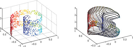
FIGURE 12.1
Left: About 950 points sampled from a Swiss roll with a hole. The color varies with respect to the spiral radius. Right: a 20-by-30 SOM learned on the Swiss roll sample.

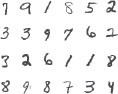
FIGURE 12.2
Examples of scanned handwritten digits randomly drawn from the MNIST database. Each image is 28 pixels wide and 28 pixels high. Gray levels range from 0 to 1.

For both data sets, two-dimensional representations are computed with NLDR methods. In the case of the Swiss roll, the embedding dimensionality is thus in agreement with the intrinsic dimensionality of the underlying manifold. In contrast, the degrees of freedom in the MNIST data base are expected to be much more numerous, and a good 2D visualization is much more difficult to obtain.

12.8.3 Methods

The compared methods are CMMDS, Sammon’s NLM, CCA, Isotop, a 20-by-30 SOM, LLE, Laplacian eigenmaps, and MVU. The first four methods are used successively with Euclidean distances and geodesic distances. The latter are computed with K-ary neighborhoods, where K = 7. All data points outside of the largest connected component are discarded. The same value of K is used for other methods involving K-ary neighborhoods (LLE and Laplacian eigenmaps). In order to reduce the huge computational cost of MVU, we used the faster variant described in [74], with K = 5 and 5% of data points randomly chosen to be landmarks. All methods run with default parameter values if not otherwise specified.

12.8.4 Results

Figure 12.3 shows a visual representation of the two-dimensional embeddings of the Swiss roll obtained with the twelve considered methods. In the particular case of the SOM, only grid nodes have coordinates both in the high- and low-dimensional space. As a simple workaround to this limitation, data points are given the same coordinates as their closest grid nodes in the high-dimensional space. Grid nodes that are never selected as the closest one are shown as a blank cell. The configuration of the SOM in the data space is visible in Figure 12.1 (right).

The quality assessment curves are shown in Figure 12.4, for a neighborhood size K ranging from 1 to 300. The solid and dashed lines refer to Q_NX(K) (above, with baseline K/(N − 1)) and B_NX(K) (below, with baseline 0), respectively. As can be seen, for distance-based methods, the use of graph distances yield a better unfolding of the Swiss roll than Euclidean ones. Among these methods, CCA performs the best, followed by Sammon’s NLM and finally CMMDS. This shows that a global minimum found by a spectral optimization technique such as in CMMDS does not systematically outperform methods relying on gradient descent. Other spectral methods, such as LLE, Laplacian eigenmaps, and MVU, work well though the quality of their results is slightly lower. In particular, MVU suffers from convergence issues in its semidefinite programming step (the constraints are apparently too tight and no solution is found). The SOM achieves an intermediate performance; due to the inherent vector quantization in this method, small neighborhoods (K < 20) are not well preserved (rank information is lost for all data points sharing the same closest grid node). Back to Figure 12.3, we see that methods showing a negative value for B_NX(K) are those that are able to actually unfold the Swiss roll. Among those methods, CCA with graph distance is the only method able to faithfully render the true latent space of the Swiss roll: a rectangle with a circular hole. Other distance-based methods tend to stretch the hole; this effect is caused by an overestimation of the distances, as geodesic paths are forced to circumvent the hole.

As to the handwritten digit images, the 2D visualizations computed with the various NLDR methods are shown in Fiure. 12.5. Each visualization consists of an array of 20-by-20 bins decorated with thumbnail images. Each thumbnail is the average of all images falling in the corresponding bin. If dissimilar images are gathered in the same bin, the thumbnail looks blurred. Empty bins are left blank. The shape of the embedding provided by the SOM trivially depends on the chosen grid. As can be seen, methods relying on (stochastic) gradient descent, such as Sammon’s NLM, CCA, and Isotop, yield disc-shaped embeddings. In contrast, spectral methods involving a sparse similarity matrix such as LLE and Laplacian eigenmaps tend to produce spiky embeddings. Knowing that the data set is likely to be clustered (one cluster for each of the ten digits), the objective functions of these methods tend to increase the distances between the clusters. In Laplacian eigenmaps, this effect results from minimizing the distances between neighbors, while keeping a fixed variance for all points; this remains valid for LLE, due to their close relationship. Maximal distances from one cluster to all others are obtained in a hyper-pyramidal configuration; for ten clusters, such a configuration spans at least nine dimensions. The linear projection of a hyper-pyramid look exactly like the spiky embeddings observed in Figure 12.5, with three corners correctly represented in two dimensions and all others collapsed in the center. This reasoning is indirectly confirmed by looking at the eigenvalue spectrum involved in these methods, showing that variance actually spreads out across many dimensions. This is a fundamental difference between spectral and nonspectral methods: the former prune dimensions only after nonlinear transformation of data, whereas the latter are directly forced to work in a low-dimensional space.

Quality assessment curves are displayed in Figure 12.6. As expected, the overall performance level is lower than for the Swiss roll, as the intrinsic dimensionality of data is much higher than two. For small values of K, hardly half of the neighbors are preserved, as indicated by Q_NX(K). The best two methods are CCA with graph distances and the SOM; they outperform all others by far. For small neighborhood sizes, the SOM is hindered by its inherent vector quantization. As with the Swiss roll, the methods with the highest values of Q_NX(K) are also those with the lower B_NX(K). The third method is Isotop with graph distances. In this example, Isotop is much faster than the SOM, because the computation of closest points is much cheaper in the low-dimensional visualization space than in the high-dimensional data space. Spectral methods yield lower performances. The semidefinite programming step in MVU does not succeed in finding a satisfying solution. Sammon’s NLM with Euclidean distances performs the worst and also hardly converges.

12.9 Conclusions

Dimensionality reduction proves to be a powerful tool for data visualization and exploratory analysis. From early linear techniques such as PCA and CMMDS to modern nonlinear methods, more than a century has passed. As shown in this chapter, the use of graphs is an important breakthrough in the domain and largely contributes to a significant performance leap. Methods relying on graphs can be categorized with respect to mainly two criteria, namely, the data properties they consider (dissimilarities or similarities) and their optimization technique (spectral or nonspectral). For instance, Isomap and MVU involve graph distances (shortest paths and specifically optimized distances, respectively) and a spectral optimization (CMMDS). Sammon’s nonlinear mapping and CCA can use shortest paths as well, but they work with a pseudo-Newton optimization and stochastic gradient descent, respectively. Spectral methods based on similarities are, for instance, Laplacian eigenmaps, LLE, and their variants. Isotop and the SOM also entail similarities, but they rely on heuristic optimization schemes. Spectral methods provide strong theoretical guarantees, such as the capability to find a global minimum. In practice, however, nonspectral techniques often outperform them, thanks to a greater flexibility and the possibility to handle more relevant or more complex cost functions.

If distance preservation has been extensively investigated for quite some time, the use of similarities remains largely unexplored. Spectral methods that uses sparse matrices of pairwise similarities, such as Laplacian eigenmaps and LLE, eventually seem to be more suited to clustering problems than to dimensionality reduction. On the other hand, nonspectral methods like Isotop and the SOM lack sound theoretical foundations or are impeded by their inherent vector quantization. In the near future, progress is likely to stem from more elaborate similarity preservation schemes, such as those developed in [75, 76, 77]. There is a hope that while naturally enforcing the preservation of the local structure, carefully designed similarities [78] can also address important issues such as the phenomenon of distance concentration [79].

Bibliography

[1] I. Jolliffe, Principal Component Analysis. New York, NY: Springer-Verlag, 1986.

[2] G. Young and A. Householder, “Discussion of a set of points in terms of their mutual distances,” Psychometrika, vol. 3, pp. 19–22, 1938.

[3] W. Torgerson, “Multidimensional scaling, I: Theory and method,” Psychometrika, vol. 17, pp. 401–419, 1952.

[4] J. Lee and M. Verleysen, Nonlinear dimensionality reduction. Springer, 2007.

[5] R. Shepard, “The analysis of proximities: Multidimensional scaling with an unknown distance function (parts 1 and 2),” Psychometrika, vol. 27, pp. 125–140, 219–249, 1962.

[6] J. Kruskal, “Multidimensional scaling by optimizing goodness of fit to a nonmetric hypothesis,” Psychometrika, vol. 29, pp. 1–28, 1964.

[7] Y. Takane, F. Young, and J. de Leeuw, “Nonmetric individual differences multidimensional scaling: an alternating least squares method with optimal scaling features,” Psychometrika, vol. 42, pp. 7–67, 1977.

[8] J. Sammon, “A nonlinear mapping algorithm for data structure analysis,” IEEE Transactions on Computers, vol. CC-18, no. 5, pp. 401–409, 1969.

[9] P. Demartines and J. Hérault, “Vector quantization and projection neural network,” ser. Lecture Notes in Computer Science, A. Prieto, J. Mira, and J. Cabestany, Eds. New York: Springer-Verlag, 1993, vol. 686, pp. 328–333.

[10] ——, “Curvilinear component analysis: A self-organizing neural network for nonlinear mapping of data sets,” IEEE Transactions on Neural Networks, vol. 8, no. 1, pp. 148–154, Jan. 1997.

[11] T. Kohonen, “Self-organization of topologically correct feature maps,” Biological Cybernetics, vol. 43, pp. 59–69, 1982.

[12] M. Kramer, “Nonlinear principal component analysis using autoassociative neural networks,” AIChE Journal, vol. 37, no. 2, pp. 233–243, 1991.

[13] E. Oja, “Data compression, feature extraction, and autoassociation in feedforward neural networks,” in Artificial Neural Networks, T. Kohonen, K. Mäkisara, O. Simula, and J. Kangas, Eds. North-Holland: Elsevier Science Publishers, B.V., 1991, vol. 1, pp. 737–745.

[14] J. Mao and A. Jain, “Artificial neural networks for feature extraction and multivariate data projection,” IEEE Transactions on Neural Networks, vol. 6, no. 2, pp. 296–317, Mar. 1995.

[15] B. Schölkopf, A. Smola, and K.-R. Müller, “Nonlinear component analysis as a kernel eigenvalue problem,” Neural Computation, vol. 10, pp. 1299–1319, 1998.

[16] J. Tenenbaum, V. de Silva, and J. Langford, “A global geometric framework for nonlinear dimensionality reduction,” Science, vol. 290, no. 5500, pp. 2319–2323, Dec. 2000.

[17] S. Roweis and L. Saul, “Nonlinear dimensionality reduction by locally linear embedding,” Science, vol. 290, no. 5500, pp. 2323–2326, 2000.

[18] M. Belkin and P. Niyogi, “Laplacian eigenmaps for dimensionality reduction and data representation,” Neural Computation, vol. 15, no. 6, pp. 1373–1396, June 2003.

[19] D. Donoho and C. Grimes, “Hessian eigenmaps: Locally linear embedding techniques for highdimensional data,” in Proceedings of the National Academy of Arts and Sciences, vol. 100, 2003, pp. 5591–5596.

[20] K. Weinberger and L. Saul, “Unsupervised learning of image manifolds by semidefinite programming,” International Journal of Computer Vision, vol. 70, no. 1, pp. 77–90, 2006.

[21] L. Xiao, J. Sun, and S. Boyd, “A duality view of spectral methods for dimensionality reduction,” in Proceedings of the 23rd International Conference on Machine Learning, Pittsburg, PA, 2006, pp. 1041–1048.

[22] L. Saul and S. Roweis, “Think globally, fit locally: Unsupervised learning of nonlinear manifolds,” Journal of Machine Learning Research, vol. 4, pp. 119–155, June 2003.

[23] N. Linial, E. London, and Y. Rabinovich, “The geometry of graphs and some of its algorithmic applications,” Combinatorica, vol. 15, no. 2, pp. 215–245, 1995.

[24] G. Di Battista, P. Eades, R. Tamassia, and I. Tollis, Graph Drawing: Algorithms for the Visualization of Graphs. Prentice Hall, 1998.

[25] I. Herman, G. Melançon, and M. Marshall, “Graph visualization and navigation in information visualization: A survey,” IEEE Transactions on Visualization and Computer Graphics, vol. 6, pp. 24–43, 2000.

[26] Y. Bengio, P. Vincent, J.-F. Paiement, O. Delalleau, M. Ouimet, and N. Le Roux, “Spectral clustering and kernel PCA are learning eigenfunctions,” Département d’Informatique et Recherche Opérationnelle, Université de Montréal, Montréal, Tech. Rep. 1239, July 2003.

[27] M. Saerens, F. Fouss, L. Yen, and P. Dupont, “The principal components analysis of a graph, and its relationships to spectral clustering,” in Proceedings of the 15th European Conference on Machine Learning (ECML 2004), 2004, pp. 371–383.

[28] B. Nadler, S. Lafon, R. Coifman, and I. Kevrekidis, “Diffusion maps, spectral clustering and eigenfunction of Fokker-Planck operators,” in Advances in Neural Information Processing Systems (NIPS 2005), Y. Weiss, B. Schölkopf, and J. Platt, Eds. Cambridge, MA: MIT Press, 2006, vol. 18.

[29] M. Brand and K. Huang, “A unifying theorem for spectral embedding and clustering,” in Proceedings of International Workshop on Artificial Intelligence and Statistics (AISTATS’03), C. Bishop and B. Frey, Eds., Jan. 2003.

[30] K. Pearson, “On lines and planes of closest fit to systems of points in space,” Philosophical Magazine, vol. 2, pp. 559–572, 1901.

[31] H. Hotelling, “Analysis of a complex of statistical variables into principal components,” Journal of Educational Psychology, vol. 24, pp. 417–441, 1933.

[32] K. Karhunen, “Zur Spektraltheorie stochastischer Prozesse,” Ann. Acad. Sci. Fennicae, vol. 34, 1946.

[33] M. Loève, “Fonctions aléatoire du second ordre,” in Processus stochastiques et mouvement Brownien, P. Lévy, Ed. Paris: Gauthier-Villars, 1948, p. 299.

[34] A. Kearsley, R. Tapia, and M. Trosset, “The solution of the metric STRESS and SSTRESS problems in multidimensional scaling using newton’s method,” Computational Statistics, vol. 13, no. 3, pp. 369–396, 1998.

[35] J. Lee, A. Lendasse, N. Donckers, and M. Verleysen, “A robust nonlinear projection method,” in Proceedings of ESANN 2000, 8th European Symposium on Artificial Neural Networks, M. Verleysen, Ed. Bruges, Belgium: D-Facto public., Apr. 2000, pp. 13–20.

[36] J. Lee and M. Verleysen, “Curvilinear distance analysis versus isomap,” Neurocomputing, vol. 57, pp. 49–76, Mar. 2004.

[37] J. Peltonen, A. Klami, and S. Kaski, “Learning metrics for information visualisation,” in Proceedings of the 4th Workshop on Self-Organizing Maps (WSOM’03), Hibikino, Kitakyushu, Japan, Sept. 2003, pp. 213–218.

[38] L. Yang, “Sammon’s nonlinear mapping using geodesic distances,” in Proc. 17th International Conference on Pattern Recognition (ICPR’04), 2004, vol. 2.

[39] P. Estévez and A. Chong, “Geodesic nonlinear mapping using the neural gas network,” in Proceedings of IJCNN 2006, 2006, in press.

[40] M. Belkin and P. Niyogi, “Laplacian eigenmaps and spectral techniques for embedding and clustering,” in Advances in Neural Information Processing Systems (NIPS 2001), T. Dietterich, S. Becker, and Z. Ghahramani, Eds. MIT Press, 2002, vol. 14.

[41] T. Kohonen, Self-Organizing Maps, 2nd ed. Heidelberg: Springer, 1995.

[42] J. Lee, C. Archambeau, and M. Verleysen, “Locally linear embedding versus Isotop,” in Proceedings of ESANN 2003, 11th European Symposium on Artificial Neural Networks, M. Verleysen, Ed. Bruges, Belgium: d-side, Apr. 2003, pp. 527–534.

[43] A. Wismüiller, “The exploration machine - a novel method for data visualization,” in Lecture Notes in Computer Science. Advances in Self-Organizing Maps, 2009, pp. 344–352.

[44] M. Bernstein, V. de Silva, J. Langford, and J. Tenenbaum, “Graph approximations to geodesics on embedded manifolds,” Stanford University, Palo Alto, CA, Tech. Rep., Dec. 2000.

[45] E. Dijkstra, “A note on two problems in connection with graphs,” Numerical Mathematics, vol. 1, pp. 269–271, 1959.

[46] M. Fredman and R. Tarjan, “Fibonacci heaps and their uses in improved network optimization algorithms,” Journal of the ACM, vol. 34, pp. 596–615, 1987.

[47] F. Shang, L. Jiao, J. Shi, and J. Chai, “Robust positive semidefinite l-isomap ensemble,” Pattern Recognition Letters, vol. 32, no. 4, pp. 640–649, 2011.

[48] H. Choi and S. Choi, “Robust kernel isomap,” Pattern Recognition, vol. 40, no. 3, pp. 853–862, 2007.

[49] K. Weinberger and L. Saul, “Unsupervised learning of image manifolds by semidefinite programming,” in Proceedings of the IEEE Conference on Computer Vision and Pattern Recognition (CVPR- 04), vol. 2, Washington, DC, 2004, pp. 988–995.

[50] J. Shi and J. Malik, “Normalized cuts and image segmentation,” IEEE Transactions on Pattern Analysis and Machine Intelligence, vol. 22, no. 8, pp. 888–905, 2000.

[51] L. Yen, D. Vanvyve, F. Wouters, F. Fouss, M. Verleysen, and M. Saerens, “Clustering using a random-walk based distance measure,” in Proceedings of ESANN 2005, 13th European Symposium on Artificial Neural Networks, M. Verleysen, Ed. Bruges, Belgium: d-side, Apr. 2005, pp. 317–324.

[52] L. Grady and J. Polimeni, Discrete Calculus: Applied Analysis on Graphs for Computational Science. New York: Springer, 2010.

[53] G. Daza-Santacoloma, C. Acosta-Medina, and G. Castellanos-Dominguez, “Regularization parameter choice in locally linear embedding,” Neurocomputing, vol. 73, no. 10–12, pp. 1595–1605, 2010.

[54] Y. Linde, A. Buzo, and R. Gray, “An algorithm for vector quantizer design,” IEEE Transactions on Communications, vol. 28, pp. 84–95, 1980.

[55] J. MacQueen, “Some methods for classification and analysis of multivariate observations,” in Proceedings of the Fifth Berkeley Symposium on Mathematical Statistics and Probability. Volume I: Statistics, L. Le Cam and J. Neyman, Eds. Berkeley and Los Angeles, CA: University of California Press, 1967, pp. 281–297.

[56] E. Erwin, K. Obermayer, and K. Schulten, “Self-organizing maps: ordering, convergence properties and energy functions,” Biological Cybernetics, vol. 67, pp. 47–55, 1992.

[57] A. Ultsch, “Maps for the visualization of high-dimensional data spaces,” in Proc. Workshop on Self-Organizing Maps (WSOM 2003), Kyushu, Japan, 2003, pp. 225–230.

[58] H.-U. Bauer, M. Herrmann, and T. Villmann, “Neural maps and topographic vector quantization,” Neural Networks, vol. 12, pp. 659–676, 1999.

[59] G. Goodhill and T. Sejnowski, “Quantifying neighbourhood preservation in topographic mappings,” in Proceedings of the Third Joint Symposium on Neural Computation. University of California, Pasadena, CA: California Institute of Technology, 1996, pp. 61–82.

[60] H.-U. Bauer and K. Pawelzik, “Quantifying the neighborhood preservation of self-organizing maps,” IEEE Transactions on Neural Networks, vol. 3, pp. 570–579, 1992.

[61] M. de Bodt, E. Cottrell and M. Verleysen, “Statistical tools to assess the reliability of self-organizing maps,” Neural Networks, vol. 15, no. 8–9, pp. 967–978, 2002.

[62] K. Kiviluoto, “Topology preservation in self-organizing maps,” in Proc. Int. Conf. on Neural Networks, ICNN’96, I. N. N. Council, Ed., vol. 1, Piscataway, NJ, 1996, pp. 294–299, also available as technical report A29 of the Helsinki University of Technology.

[63] C. Bishop, M. Svensén, and K. Williams, “GTM: A principled alternative to the self-organizing map,” Neural Computation, vol. 10, no. 1, pp. 215–234, 1998.

[64] T. Martinetz and K. Schulten, “A “neural-gas” network learns topologies,” in Artificial Neural Networks, T. Kohonen, K. Mäkisara, O. Simula, and J. Kangas, Eds. Amsterdam: Elsevier, 1991, vol. 1, pp. 397–402.

[65] ——, “Topology representing networks,” Neural Networks, vol. 7, no. 3, pp. 507–522, 1994.

[66] M. Jünger and P. Mutzel, Graph Drawing Software. Springer-Verlag, 2004.

[67] J. Lee and M. Verleysen, “Nonlinear projection with the Isotop method,” in LNCS 2415: Artificial Neural Networks, Proceedings of ICANN 2002, J. Dorronsoro, Ed. Madrid (Spain): Springer, Aug. 2002, pp. 933–938.

[68] J. Venna and S. Kaski, “Neighborhood preservation in nonlinear projection methods: An experimental study,” in Proceedings of ICANN 2001, G. Dorffner, H. Bischof, and K. Hornik, Eds. Berlin: Springer, 2001, pp. 485–491.

[69] L. Chen and A. Buja, “Local multidimensional scaling for nonlinear dimension reduction, graph drawing, and proximity analysis,” Journal of the American Statistical Association, vol. 101, no. 485, pp. 209–219, 2009.

[70] J. Lee and M. Verleysen, “Rank-based quality assessment of nonlinear dimensionality reduction,” in Proceedings of ESANN 2008, 16th European Symposium on Artificial Neural Networks, M. Verleysen, Ed. Bruges: d-side, Apr. 2008, pp. 49–54.

[71] ——, “Quality assessment of nonlinear dimensionality reduction based on k-ary neighborhoods,” in JMLR Workshop and Conference Proceedings (New challenges for feature selection in data mining and knowledge discovery), Y. Saeys, H. Liu, I. Inza, L. Wehenkel, and Y. Van de Peer, Eds., Sept. 2008, vol. 4, pp. 21–35.

[72] ——, “Quality assessment of dimensionality reduction: Rank-based criteria,” Neurocomputing, vol. 72, no. 7–9, pp. 1431–1443, 2009.

[73] Y. LeCun, L. Bottou, Y. Bengio, and P. Haffner, “Gradient-based learning applied to document recognition,” Proceedings of the IEEE, vol. 86, no. 11, pp. 2278–2324, Nov. 1998.

[74] K. Weinberger, B. Packer, and L. Saul, “Nonlinear dimensionality reduction by semidefinite programming and kernel matrix factorization,” in Proceedings of the Tenth International Workshop on Artificial Intelligence and Statistics (AISTATS 2005), R. Cowell and Z. Ghahramani, Eds. Bardados: Society for Artificial Intelligence and Statistics, Jan. 2005, pp. 381–388.

[75] G. Hinton and S. Roweis, “Stochastic neighbor embedding,” in Advances in Neural Information Processing Systems (NIPS 2002), S. Becker, S. Thrun, and K. Obermayer, Eds. MIT Press, 2003, vol. 15, pp. 833–840.

[76] L. van der Maaten and G. Hinton, “Visualizing data using t-SNE,” Journal of Machine Learning Research, vol. 9, pp. 2579–2605, 2008.

[77] J. Venna, J. Peltonen, K. Nybo, H. Aidos, and S. Kaski, “Information retrieval perspective to nonlinear dimensionality reduction for data visualization,” Journal of Machine Learning Research, vol. 11, pp. 451–490, 2010.

[78] J. A. Lee and M. Verleysen, “Shift-invariant similarities circumvent distance concentration in stochastic neighbor embedding and variants,” in Proc. International Conference on Computational Science (ICCS 2011), Singapore, 2011.

[79] D. François, V. Wertz, and M. Verleysen, “The concentration of fractional distances,” IEEE Transactions on Knowledge and Data Engineering, vol. 19, no. 7, pp. 873–886, July 2007.

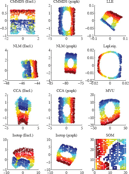
FIGURE 12.3
Two-dimensional embeddings of the Swiss roll with various NLDR methods. Distance-based methods use either Euclidean norm (‘Eucl.’) or shortest paths in a neighborhood graph (‘Graph’).

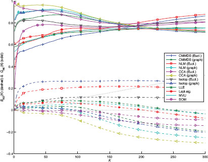
FIGURE 12.4
Quality assessment curves for the two-dimensional embeddings of the Swiss roll with various NLDR methods.

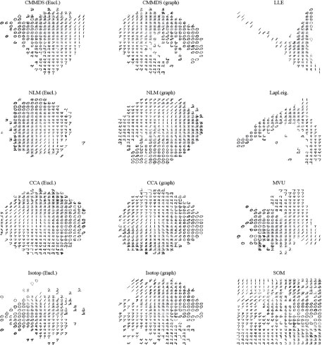
FIGURE 12.5
Two-dimensional embeddings of the handwritten digits with various NLDR methods. Distance-based methods use either Euclidean norm (‘Eucl.’) or shortest paths in a neighborhood graph (‘Graph’).

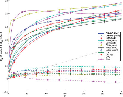
FIGURE 12.6
Quality assessment curves for the two-dimensional embeddings of the handwritten digits with various NLDR methods.

..................Content has been hidden....................

You can't read the all page of ebook, please click here login for view all page.

Table of Contents for 12 Graph-Based Dimensionality Reduction

Create new playlist

Sign In

Sign Up

Table of Contents for
12 Graph-Based Dimensionality Reduction