13 Graph Edit Distance—Theory, Algorithms, and Applications

Graphs provide us with a powerful and flexible representation formalism which can be employed in various fields of intelligent information processing. Graph matching refers to the process of evaluating the similarity between graphs. Two approaches to this task have been proposed, namely, exact and inexact (or error-tolerant) graph matching. While the former approach aims at finding a strict correspondence between two graphs to be matched, the latter is able to cope with errors and measures the difference of two graphs in a broader sense. As a matter of fact, inexact graph matching has been a highly significant research topic in the area of pattern analysis for a long time. The graph edit distance (GED) is a foundation of inexact graph matching, and has emerged as an important way to measure the similarity between pairs of graphs in an error-tolerant fashion.

13.1 Introduction

One of the basic objectives in pattern recognition is to develop systems for the analysis or classification of objects [1, 2]. In principle, these objects or patterns can be of any kind. For instance, they can include images taken from a digital camera, speech signals captured with a microphone, or words written with a pen or a tablet PC, to name a few. A first issue to be addressed in any pattern recognition system is how to represent these objects. Feature vectors is one of the most common and widely used data representations. That is, for each object, a set of relevant properties, or features, are extracted and arranged in a vector. Then, a classifier can be trained to recognize the unknown objects. The main advantage of this representation is that a large number of algorithms for pattern analysis and classification become immediately available [1]. This is mainly due to the fact that vectors are simple structures that have many interesting and useful mathematical properties.

However, some disadvantages arise from the simple structure of feature vectors. Regardless of the complexity of the object, within one particular application, feature vectors have always to have the same length and structure (a simple list of predetermined components). Therefore, for the representation of complex objects where the relations between their parts become important for their analysis or classification, graphs appear as an appealing alternative. One of the main advantages of graphs over feature vectors is that graphs can explicitly model relations between different parts of an object, whereas feature vectors are only able to describe an object as an aggregation of numerical properties. In addition, graphs permit us to associate any kind of label (not only numbers) to both edges and nodes, extending in this way the spectrum of properties that can be represented. Furthermore, the dimensionality of graphs, that is, the number of nodes and edges, can be different for every object, even for objects of the same class. Thus, the more complex an object is, the larger the number of nodes and edges can be.

Although these visible differences between graphs and vectors exist, one can see from the literature that vector and graph representations are not mutually exclusive. For instance, there is a substantial literature in complex networks that characterizes the graph structure by means of feature vectors using different measures on graphs, such as connectivity and average distance. Two surveys on that field are [3, 4]. Recently, an extensive work comparing the representational power of feature vectors and graphs without restrictions in the node labels under the context of Web content mining has been presented in [5]. Experimental results consistently show an improvement in the accuracy of the graph-based approaches over comparable vector-based methods. In addition, in some cases the experiments even showed an improvement in execution time over the vector model.

Actually, graphs have been used to solve computer vision problems for decades. Some examples include recognition of graphical symbols [6, 7], character recognition [8, 9], shape analysis [10, 11], 3D-object recognition [12, 13], and video and image database indexing [14]. However, in spite of the strong mathematical foundation underlying graphs and their high power of representation, working with graphs is usually harder and more challenging than working with feature vectors.

Graph matching is the specific process of evaluating the structural similarity of two graphs¹^,². It can be split into two categories, namely exact and error-tolerant graph matching. In exact graph matching, the basic objective is to decide whether two graphs or parts of them are identical in terms of their structure and labels. Methods for exact graph matching include graph isomorphism, subgraph isomorphism [15], maximum common subgraph [16], and minimum common supergraph [17]. The main advantage of exact graph matching methods is their stringent definition and solid mathematical foundation. Nevertheless, it is still imperative for the underlying graphs to share isomorphic parts to be considered similar. This means that the two graphs under comparison must be identical to a large extent in terms of structure and labels to produce high similarity values. In practice, node and edge labels used to describe the properties of the underlying objects (represented by the graphs) are often of continuous nature. In this situation, at least two problems arise. First, it is not sufficient to check whether two labels are identical or not, but one has also to evaluate their similarity. In addition, under all the matching procedures mentioned so far, two labels will be considered different regardless of the degree of difference between them. This may lead to considering two graphs with similar, but not identical labels completely dissimilar even if they have identical structure. It is therefore clear that a more sophisticated method is needed to measure the dissimilarity between graphs, taking into account such limitations. This leads to the definition of inexact, or error-tolerant, graph matching.

In error-tolerant graph matching, the idea is to evaluate the similarity of two graphs in a broader sense that better reflects the intuitive understanding of graph similarity. In fact, error-tolerant graph matching methods need not be defined by means of a graph similarity measure at all, but can be formulated in entirely different terms. In the ideal case, two graphs representing the same class of objects are identical. That is, a graph extraction process turning objects into graphs should always result in exactly the same graph for objects of the same class. In practice, of course, the graph extraction process suffers from noise and various distortions. In graph matching, error-tolerance means that the matching algorithm is able to cope with the structural difference between the actually extracted graph and the ideal graph.

In this chapter, we review a number of exact and error-tolerant graph distance measures. The main focus is the graph edit distance (GED), which is recognized as one of the most flexible and universal error-tolerant matching paradigm. Graph edit distance is not constrained to particular classes of graphs and can be tailored to specific applications. The main restriction is that the computation of edit distance is inefficient, particularly for large graphs. Recently, however, faster approximate solutions have become available (see Section 13.4) This chapter is devoted to a detailed description of graph edit distance. We review the graph edit distance from three different points of view, namely, theory, algorithms, and applications. In the first part of the chapter, fundamental concepts related to GED are introduced. Special emphasis will be put on the theory underlying the edit distance cost function, giving some examples and introducing the fundamental problem of automatic edit cost learning. The second part of the chapter gives an introduction to GED computation. We review in detail exact and approximate methods for GED computation and finish by introducing one of the most recent approximate algorithms for GED computation, which is based on bipartite graph matching. The last part of the chapter is devoted to GED applications. We concentrate on three basic applications: the weighted mean of a pair of graphs, graph embedding into vector spaces, and the median graph computation problem. We finish the chapter by giving some conclusions and pointing to future directions in GED theory and practice.

13.2 Definitions and Graph Matching

Definition 13.2.1

Graph: Given L, a finite or infinite set of labels for nodes and edges, a graph $G$ is defined by the tuple $G = (V, ℰ)$ where,

• $V$ is a finite set of nodes

• $ℰ \subseteq V \times V$ is the set of edges³

Without loss of generality, Definition 13.2.1 can be seen as the definition of a labeled graph. Notice that there is not any restriction concerning the nature of the labels of nodes and edges. That is, the label alphabet is not constrained at all. L may be defined as a vector space (i.e. $L = ℝ^{n}$ ) or simply as a finite or infinite set of discrete labels (i.e., L = {α, β, γ, ⋯ }). The set of labels L can also include the null label (often represented by ε). If all the nodes and edges are labeled with the same null label, the graph is considered as unlabeled. A weighted graph is a special type of labeled graph in which each node is labeled with the null label and each edge (υ_i, υ_j) is labeled with a real number or weight w_ij, usually belonging, but not restricted, to the interval [0, 1]. An unweighted graph can be seen as a particular instance of a weighted graph where ∀(v_i,v_j) ∈ $E$ , w_ij = 1. The label of an element ● (where ● can be a node or an edge) is denoted by L(●).

In the more general case, vertices and edges may represent more complex information. That is, they can contain information of a different nature at the same time. For instance, a complex attribute for a node representing a region of an image could be composed of the color histogram of the region, a description of its shape and symbolic information relating this region with its adjacent regions. In this case graphs are called attributed graphs or simply AG. Notice that labeled, weighted, and unweighted graphs are particular instances of attributed graphs, where the attributes are simple labels or numbers.

Definition 13.2.2

Subgraph: Let $G_{1} = (V_{1}, ℰ_{1})$ , and $G_{2} = (V_{2}, ℰ_{2})$ be two graphs. Graph $G_{1}$ is a subgraph of $G_{2}$ , denoted by $G_{1} = G_{2}$ , if

• $V_{1} \subseteq V_{2}$

• $ℰ_{1} = ℰ_{2} \cap (V_{1} \times V_{1})$

From Definition 13.2.2 it follows that, given a graph $G = (V, ℰ)$ , a subset $V^{'} \subseteq V$ of its vertices uniquely defines a subgraph, called the subgraph induced by $V^{'}$ . That is, an induced subgraph of S can be obtained by removing some of its nodes $(V - V^{'})$ and all their adjacent edges. However, if the second condition of Definition 13.2.2 is replaced by $ℰ_{1} \subseteq ℰ_{2}$ then the resulting subgraph is called noninduced. A noninduced subgraph of $G$ is obtained by removing some of its nodes $(V - V^{'})$ and all their adjacent edges plus some additional edges. An example of a graph $G$ , an induced, and a noninduced subgraph of $G$ is given in Figure 13.1 (note that node labels are represented using different shades of grey). Of course, given a graph $G$ , an induced subgraph of $G$ is also a noninduced subgraph of $G$ .

13.2.1 Exact Graph Matching

The operation of comparing two graphs is commonly referred to as graph matching. The aim of exact graph matching is to determine whether two graphs, or parts of two graphs, are identical in terms of their structure and labels. The equality of two graphs can be tested by means of a bijective function, called graph isomorphism, defined as follows:

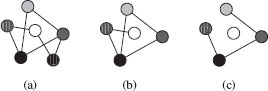
FIGURE 13.1
Original model graph $G$ (a), an induced subgraph of $G$ (b) and a non-induced subgraph of $G$ (c).

Definition 13.2.3

Graph isomorphism: Let $G_{1} = (V_{1}, ℰ_{1})$ and $G_{2} = (V_{2}, ℰ_{2})$ be two graphs. A graph isomorphism between $G_{1}$ and $G_{2}$ is a bijective mapping $f : V_{1} \to V_{2}$ such that

• L(υ) = L(f(υ)) for all nodes $υ \in V_{1}$

• for each edge $e_{1} = (υ_{i}, υ_{j}) \in ℰ_{1}$ , there exists an edge $e_{2} = (f (υ_{i}), f (υ_{j})) \in ℰ_{2}$ such that L(e₁) = L(e₂)

• for each edge $e_{2} = (υ_{i}, υ_{j}) \in ℰ_{2}$ , there exists an edge $e_{1} = (f^{- 1} (υ_{i}), f^{- 1} (υ_{j})) \in ℰ_{1}$ such that L(e₁) = L(e₂)

It is clear from this definition that isomorphic graphs are identical in terms of structure and labels. To check whether two graphs are isomorphic or not, we have to find a function mapping every node of the first graph to a node of the second graph in such a way that the edge structure of both graphs is preserved, and the labels for the nodes and the edges are consistent. Graph isomorphism is an equivalence relation on graphs, since it satisfies the conditions of reflexivity, symmetry, and transitivity.

Related to graph isomorphism is the concept of subgraph isomorphism. It permits one to check whether a part (subgraph) of one graph is identical to another graph. A subgraph isomorphism exists between two given graphs $G_{1}$ and $G_{2}$ if there is a graph isomorphism between the smaller graph and a subgraph of the larger graph, i.e., if the smaller graph is contained in the larger graph. Formally, subgraph isomorphism is defined as follows:

Definition 13.2.4

Subgraph Isomorphism: Let $G_{1} = (V_{1}, ℰ_{1})$ and $G_{2} = (V_{2}, ℰ_{2})$ be two graphs. An injective function $f : V_{1} \to V_{2}$ is called a subgraph isomorphism from $G_{1}$ to $G_{2}$ if there exists a subgraph $G \subseteq G_{2}$ , such that f is a graph isomorphism between $G_{1}$ and $G$ .

Most of the algorithms for graph isomorphism and subgraph isomorphism are based on some form of tree search with backtracking. The main idea is to iteratively expand a partial match (initially empty) by adding new pairs of nodes satisfying some constraints imposed by the matching method with respect to the previously matched pairs of nodes. These methods usually apply some heuristic conditions to prune useless search paths as early as possible. Eventually, either the algorithm finds a complete match or reaches a point where the partial match cannot be further expanded because of the matching constraints. In the latter case, the algorithm backtracks until it finds a partial match for which another alternative expansion is possible. The algorithm halts when all the possible mappings that satisfy the constraints have been tried.

One of the most important algorithms based on this approach is described in [15]. It addresses both the graph and subgraph isomorphism problem. To prune unfruitful paths at an early stage, the author proposes a refinement procedure that drops pairs of nodes that are inconsistent with the partial match being explored. The branches of this partial match leading to these incompatible matches are not expanded. A similar strategy is used in [18], where the authors include an additional preprocessing step that creates an initial partition of the nodes of the graph based on a distance matrix to reduce the size of the search space. More recent approaches are the VF [19] and the VF2 [20] algorithms. In these works, the authors define a heuristic based on the analysis of the nodes adjacent to the nodes of the partial mapping. This procedure is fast to compute and leads in many cases to an improvement over the approach of [15]. Another recent approach which combines explicit search in state-space and the use of energy minimization is [21]. The basic heuristic of this algorithm can be interpreted as a greedy algorithm to form maximal cliques in an association graph. In addition, the authors allow for vertex swaps during the clique creation. This last characteristic makes this algorithm faster than a PBH (pivoting-based heuristic).

Probably, the most important approach to graph isomorphism testing that is not based on tree search is described in [22]. It uses concepts from group theory. First, the automorphism group of each input graph is constructed. After that, a canonical labelling is derived and isomorphism is checked by simply verifying the equality of the canonical forms.

It is still an open question whether the graph isomorphism problem belongs to the NP class or not. Polynomial algorithms have been developed for special classes of graphs such as bounded valence graphs [23] (i.e., graphs where the maximum number of edges adjacent to a node is bounded by a constant); planar graphs [24] (i.e., graphs that can be drawn on a plane without graph edges crossing) and trees [11] (i.e., graphs with no cycles). But no polynomial algorithms are known for the general case. Conversely, the subgraph isomorphism problem is proven to be NP-complete [25].

Matching graphs by means of graph and subgraph isomorphism is limited in the sense that an exact correspondence must exist between two graphs or between a graph and part of another graph. But let us consider the situation of Figure 13.2(a). It is clear that the two graphs are similar, since most of their nodes and edges are identical. But it is also clear that none of them is related to the other one by (sub)graph isomorphism. Therefore, under the (sub)graph isomorphism paradigm, they will be considered completely different graphs. Consequently, in order to overcome such a drawbacks of the (sub)graph isomorphism, to establish a measure of partial similarity between any two graphs, and to relax this rather stringent condition, the concept of the largest common part of two graphs is introduced.

Definition 13.2.5

Maximum common subgraph (MACS): Let $G_{1} = (V_{1}, ℰ_{1})$ and $G_{2} = (V_{2}, ℰ_{2})$ be two graphs. A graph $G$ is called a common subgraph (cs) of $G_{1}$ and $G_{2}$ if there exists a subgraph isomorphism from $G$ to $G_{1}$ and from $G$ to $G_{2}$ . A common subgraph of $G_{1}$ and $G_{2}$ is called maximum common subgraph (MACS) if there exists no other common subgraph of $G_{1}$ and $G_{2}$ with more nodes than $G$ .

The notion of maximum common subgraph of two graphs can be interpreted as an intersection. Intuitively, it is the largest part of either graph that is identical in terms of structure and labels. It is clear that the larger the maximum common subgraph is, the more similar the two graphs are.

Macs computation has been intensively investigated. There are two major approaches in the literature. In [16, 26, 27] a backtracking search is used. A different strategy is proposed in [28, 29], where the authors reduce the MACS problem to the problem of finding a maximum clique (i.e., a completely connected subgraph) of a suitably constructed association graph [30]. A comparison of some of these methods on large databases of graphs is given in [31, 32].

It is well known that the MACS and the maximum clique problems are NP-complete. Therefore, some approximate algorithms have been developed. A survey of these approximate approaches and the study of their computational complexity is given in [33]. Nevertheless, in [34] it is shown that when graphs have unique node labels, the computation of the MACS can be done in polynomial time. This important result has been exploited in [5] to perform data mining on Web pages based on their contents. Other applications of the MACS include comparison of molecular structures [35, 36] and matching of 3-D graph structures [37].

Dual to the definition of the maximum common subgraph (interpreted as an intersection operation) is the concept of the minimum common supergraph.

Definition 13.2.6

(Minimum common supergraph (MICS)): Let $G_{1} = (V_{1}, ℰ_{1})$ and $G_{2} = (V_{2}, ℰ_{2})$ be two graphs. A graph $G$ is called a common supergraph (CS) of $G_{1}$ and $G_{2}$ if there exists a subgraph isomorphism from $G_{1}$ to $G$ and from $G_{2}$ to $G$ . A common supergraph of $G_{1}$ and $G_{2}$ is called minimum common supergraph (MICS) if there exists no other common supergraph of $G_{1}$ and $G_{2}$ with less nodes than $G$ .

The minimum common supergraph of two graphs can be seen as a graph with the minimum required structure so that both graphs are contained in it as subgraphs. In [17], it is demonstrated that the computation of the minimum common supergraph can be reduced to the computation of the maximum common subgraph. This result has not only relevant theoretical implications, but also practical consequences in the sense that any algorithm for the MACS computation, such as all algorithms described before, can also be used to compute the MICS.

An example of the concepts of MACS and MICS is given in Figure 13.2. Notice that, in general, neither MACS $(G_{1}, G_{2})$ nor MICS $(G_{1}, G_{2})$ are uniquely defined for two given graphs $G_{1}$ and $G_{2}$ .

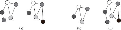
FIGURE 13.2
Two graphs $G_{1}$ and $G_{2}$ (a), MACS $(G_{1}, G_{2})$ (b) and MICS $(G_{1}, G_{2})$ (c).

13.2.1.1 Graph Similarity Measures Based on the MACS and the MICS

The concepts of maximum common subgraph and minimum common supergraph can be used to measure the similarity of two graphs. The basic idea is the intuitive observation that the larger the common part of two graphs is, the higher their similarity. In the following, several distance measures between graphs based on the concepts of the MACS and the MICS will be presented.

For instance, in [38] a distance metric between two graphs is defined in the following way:

$d_{1} (G_{1}, G_{2}) = | G_{1} | + | G_{2} | - 2 | MACS (G_{1}, G_{2}) |$

(13.1)

It is clear in this definition that, if two graphs are similar, they will have a $MACS (G_{1}, G_{2})$ similar to both of them. Then, the term $| MACS (G_{1}, G_{2}) |$ will be close to $| G_{1} |$ and $| G_{2} |$ and therefore the distance close to 0. Conversely, if the graphs are dissimilar, the term $| MACS (G_{1}, G_{2}) |$ will tend to 0 and the distance will be large.

Another distance measure based on the MACS [39] is

$d_{2} (G_{1}, G_{2}) = 1 - \frac{| MACS (G_{1}, G_{2}) |}{\max (| G_{1} |, | G_{2} |)}$

(13.2)

In this case, if the two graphs are very similar, then their maximum common subgraph will obviously be almost as large as one of the two graphs. Then, the value of the fraction will therefore tend to 1 and the distance will be close to 0. For two dissimilar graphs, their maximum common subgraph will be small, and the ratio will then be close to 0 and the distance close to 1. Clearly, the distance metric d₂ is bounded between 0 and 1, and the more similar two graphs are the smaller is d₂.

A similar distance is defined in [40], but the union graph is used as a normalization factor instead of the size of the larger graph,

$d_{3} (G_{1}, G_{2}) = 1 - \frac{| MACS (G_{1}, G_{2}) |}{| G_{1} | + | G_{2} | - | MACS (G_{1}, G_{2}) |}$

(13.3)

By “graph union”, the authors of [40] mean that the denominator represents the size of the union graph in the set theory point of view. As a matter of fact, this denominator is equal to $| MICS (G_{1}, G_{2}) |$ . The behaviour of distance d₃ is similar to that of d₂. The use of the graph union is motivated by the fact that changes in the size of the smaller graph that keep the $MACS (G_{1}, G_{2})$ constant are not taken into account in d₂, whereas distance d₃ does take this variations into account. This measure was also demonstrated to be a metric and gives a distance value in the interval [0, 1].

Another approach based on the difference between the minimum common supergraph and the maximum common subgraph was proposed in [41]. In this approach, the distance is given by

$d_{4} (G_{1}, G_{2}) = | MICS (G_{1}, G_{2}) | - | MACS (G_{1}, G_{2}) |$

(13.4)

The basic idea is that for similar graphs, the size of the maximum common subgraph and the minimum common supergraph will be similar, and the resulting distance will be small. On the other hand, if the graphs are dissimilar, the two terms will be significantly different, resulting in larger distance values. It is important to notice that also d₄ is a metric. In fact, it can be easily shown that this distance is equal to d₁.

Obviously, the similarity measures d₁ to d₄ admit a certain amount of error-tolerance. That is, with the use of these similarity measures, two graphs do not need to be directly related in terms of (sub)graph isomorphism to be successfully matched. Nevertheless, it is still imperative for these graphs to share isomorphic parts to be considered similar. This means that the two graphs must be identical to a large extent in terms of structure and labels to produce large values of the similarity measures. In many practical applications, however, node and edge labels used to describe the properties of the underlying objects (represented by graphs) are of continuous nature. In this situation, at least two problems emerge. First, it is not sufficient to evaluate whether two labels are identical or not, but one has to evaluate their similarity. In addition, using all the distances given so far, two labels will be considered different, regardless of the actual degree of dissimilarity between them. This may lead to the problem of considering two graphs with similar, but not identical, labels completely different, even if they have identical structure. It is therefore clear that there is a need of a more sophisticated method to measure the dissimilarity between graphs, which takes into account such limitations. This leads to the definition of inexact or error-tolerant graph matching.

13.2.2 Error-Tolerant Graph Matching

The methods for exact graph matching outlined above have solid mathematical foundation. Nevertheless, their stringent conditions restrict their applicability to a very small range of real-world problems only. In many practical applications, when objects are encoded using graph-based representations, some degree of distortion may occur due to multiple reasons. For instance, there may exist some form of noise in the acquisition process, nondeterministic elements in some of the processing steps, etc. Hence, graph representations of the same object may differ somewhat, and two identical objects may not have an exact match when transformed into their graph-based representations. Therefore, it is necessary to introduce some degree of error tolerance into the matching process, so that structural differences between the models can be taken into account. For this reason, a number of error-tolerant, or inexact, graph matching methods have been proposed. They deal with a more general graph matching problem than (sub)graph isomorphism, the MACS, and the MICS problem.

The key idea of error-tolerant graph matching is to measure the similarity between two given graphs instead of simply giving an indication of whether they are identical or not. Usually, in these algorithms the matching between two different nodes that do not preserve the edge compatibility is not forbidden. But a cost is introduced to penalize the difference. The task of any related algorithm is then to find the mapping that minimizes the matching cost. For instance, an error-tolerant graph matching algorithm is expected to discover not only that the graphs in the Figure 13.2(a) share some parts of their structure but also that they are rather similar despite the difference in their structure.

As in the case of exact matching, techniques based on tree search can also be used for inexact graph matching. Differently from exact graph matching where only identical nodes are matched, in this case, the search is usually controlled by the partial matching cost obtained so far and a heuristic function to estimate the cost of matching the remaining nodes. The heuristic function is used to prune unsuccessful paths in a depth-first search approach or to determine the order in which the search tree has to be traversed by an A* algorithm. For instance, the use of an A* strategy is proposed in [42] to obtain an optimal algorithm to compute the graph distance. In [43] an A*-based approach is used to cast the matching between two graphs as a bipartite matching problem. A different approach is used in [44], where the authors present an inexact graph matching method that also exploits some form of contextual information, defining a distance between function described graphs (FDG). Finally, a parallel branch and bound algorithm has been presented in [45] to compute a distance between two graphs with the same number of nodes.

Another class of approaches to inexact graph matching are those based on genetic algorithms [46, 47, 48, 49, 50]. The main advantage of genetic algorithms is that they are able to cope with huge search spaces. In genetic algorithms, the possible solutions are encoded as chromosomes. These chromosomes are generated randomly following some operators inspired by evolution theory, such as mutation and crossover. To determine how good a solution (chromosome) is, a fitness function is defined. The search space is explored with a combination of the fitness function and the randomness of the biologically inspired operators. The algorithm tends to favour well-performing candidates with a high value of the fitness function. The two main drawbacks of genetic algorithms are that they are nondeterministic algorithms and that the final output is dependent on the initialization phase. On the other hand, these algorithms are able to cope with difficult optimization problems and they have been widely used to solve NP-complete problems [51]. For instance, in [48] the matching between two given graphs is encoded in a vector form as a set of node-to-node correspondences. Then an underlying distortion model (similar to the idea of cost function presented in the next section) is used to evaluate the quality of the match by simply accumulating individual costs.

Spectral methods [52, 53, 54, 55, 56, 57, 58] have also been used for inexact graph matching. The basic idea of these methods is to represent graphs by the eigen-decomposition of their adjacency or Laplacian matrix. Among the pioneering works of the spectral graph theory applied to graph matching problems is [56]. This work proposes an algorithm for the weighted graph isomorphism problem, where the objective is to match a subset of nodes of the first graph to a subset of nodes of the second graph, usually by means of a matching matrix M. One of the major limitations of this approach is that the graphs must have the same number of nodes. A more recent paper [58] proposes a solution to the same problem by combining the use of eigenvalues and eigenvectors with continuous optimization techniques. In [59] some spectral features are used to cluster sets of nodes that are likely to be matched in an optimal correspondence. This method does not suffer from the limitation of [56] that all graphs must have the same number of nodes. Another approach combining clustering and spectral graph theory has been presented in [60]. In this approach the nodes are embedded into a so-called graph eigenspace using the eigenvectors of the adjacency matrix. Then, a clustering algorithm is used to find nodes of the two graphs that are to be put in correspondence. A work that is partly related to spectral techniques has been proposed in [61, 55]. Here, the authors assign a Topological Signature Vector, or TSV, to each nonterminal node of a directed acyclic graph (DAG). The TSV associated to a node is based on the sum of the eigenvalues of its descendant DAGs. It can be seen as a signature to represent the shape of an object and can be used both for indexing graphs in a database and for graph matching [62].

A completely different approach is to cast the inexact graph matching problem as a nonlinear optimization problem. The first family of methods based on this idea is relaxation labelling [63, 64]. The main idea is to formulate the matching of the two graphs under consideration as a labeling problem. That is, each node of one of the graphs is to be assigned to one label out of all the possible labels. This label determines the corresponding node of the other graph. To model the compatibility of the node labeling, a Gaussian probability distribution is used. In principle, only the labels attached to the nodes or the nodes together with their surrounding edges can be taken into consideration in this probability distribution. Then, the labelling is iteratively refined until a sufficiently accurate labelling is found. Any node assignment established in this way implies an assignment of the edges between the two graphs. In another approach described in [65], the nodes of the input graph are seen as the observed data while the nodes of the model graph act as hidden random variables. The iterative matching process is handled by the expectation-maximization algorithm [66]. Finally, in another classical approach [67], the problem of weighted graph matching is tackled using a technique called graduated assignment which makes it possible to avoid poor local optima.

In the last paragraphs we have described some of the most relevant algorithms for error-tolerant graph matching. Relaxation methods, graduate assignment, spectral method,s etc. can be used to establish a mapping between the nodes and edges of the two graphs, but do not directly give us any distances or dissimilarities as they are required by a classifier or clustering algorithm. In the next section we review graph edit distance, which is one of the most widely used error-tolerant graph matching methods. Differently from other methods, edit distance is suitable to compute graph distances. As far as the computational complexity is concerned, any of the graph matching problems, subgraph isomorphism, maximum common subgraph, edit distance, etc. are NP complete. Hence computational tractability is an issue for all of them. However, no experimental comparison has been conducted to directly compare all of these methods with respect to performance and efficiency. An excellent review of algorithms for both exact and error-tolerant graph matching can be found in [68].

13.2.3 Graph Edit Distance

The basic idea behind the graph edit distance is to define a dissimilarity measure between two graphs by the minimum amount of distortion required to transform one graph into the other [69, 70, 71, 72]. To this end, a number of distortions or edit operations ed, consisting of the insertion, deletion, and substitution (replacement of a label by another one) of both nodes and edges are defined. Then, for every pair of graphs, $G_{1}$ and $G_{2}$ , there exists a sequence of edit operations, or edit path $\partial (G_{1}, G_{2}) = (e d_{1}, \dots, e d_{k})$ (where each ed_i denotes an edit operation), that transform one graph into the other. In Figure 13.3, an example of an edit path between two given graphs $G_{1}$ and $G_{2}$ is shown. In this example, the edit path consists of one edge deletion, one node substitution, one node insertion, and two edge insertions.

In general, several edit paths may exist between two given graphs. This set of edit paths is denoted by $℘ (G_{1}, G_{2})$ . To quantitatively evaluate which is the best edit path, an edit cost function is introduced. The basic idea is to assign a cost c to each edit operation according to the amount of distortion that it introduces in the transformation. The edit distance between two graphs $G_{1}$ and $G_{2}$ , denoted by $d (G_{1}, G_{2})$ , is defined by the minimum cost edit path that transforms one graph into the other.

Definition 13.2.7

Graph Edit Distance: Given two graphs $G_{1} = (V_{1}, ℰ_{1})$ , and $G_{2} = (V_{2}, ℰ_{2})$ , the graph edit distance between $G_{1}$ and $G_{2}$ is defined by:

$d (G_{1}, G_{2}) = \min_{(e d_{1}, \dots, e d_{k}) \in ℘ (G_{1}, G_{2})} \sum_{i = 1}^{k} c (e d_{i})$

(13.5)

where $℘ (G_{1}, G_{2})$ denotes the set of edit paths that transform $G_{1}$ into $G_{2}$ and c(ed) denotes the cost of an edit operation ed.

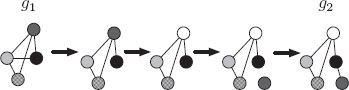
FIGURE 13.3
A possible edit path between two graphs $G_{1}$ and $G_{2}$ .

13.3 Theoretical Aspects of GED

In this section we introduce some theoretical aspects concerning the graph edit distance. We first introduce some important aspects related to the edit costs that may affect the result with respect to the underlying application. Then, we briefly show how these edit costs can be learnt automatically.

13.3.1 Edit Costs

One of the key components of the graph edit distance is the costs of the edit operations. Edit operation costs specify how expensive it is to apply a node deletion and a node insertion instead of a node substitution, and if node operations are more important than edge operations. In this context, it is clear that the underlying graph representation must be taken into account in order to define edit costs in an appropriate way. For some representations, nodes and their labels may be more important than edges. For other representations, for example, in a network monitoring application, where a missing edge represents a broken physical link, it may be crucial whether or not two nodes are linked by an edge. Thus, in order to obtain a suitable graph edit distance measure, it is of key importance to define the edit costs in such a way that the structural variations of graphs are modeled according to the given domain. In other words, the definition of the edit costs strongly depends on the underlying application.

13.3.1.1 Conditions on Edit Costs

In the definition of edit distance given above, the distance $d (G_{1}, G_{2})$ between two graphs has been defined over the set $℘ (G_{1}, G_{2})$ formed by all the edit paths from $G_{1}$ to $G_{1}$ . Theoretically, one could take a valid edit path ∂ from ℘ and construct an infinite number of edit paths from ∂ by arbitrarily inserting and deleting a single node, making the cardinality of ℘ infinite. However, as we will show, if the edit cost function satisfies a few weak conditions, it is enough to evaluate a finite subset of edit paths from ℘ to find one with minimum cost among all edit paths. The first condition we require on the edit costs is the nonnegativity,

$c (e d) \geq 0$

(13.6)

for all node and edge edit operations ed.

This condition is certainly reasonable since edit costs are usually seen as distortions or penalty costs associated with their edit operations. The next conditions account for unnecessary substitutions. They state that removing unnecessary substitutions from an edit path does not increase the sum of the edit operation cost,

$c (u \to w) \leq c (u \to υ) + c (υ \to w)$

(13.7)

$c (u \to ϵ) \leq c (u \to υ) + c (υ \to ϵ)$

(13.8)

$c (ϵ \to υ) \leq c (ϵ \to u) + c (u \to υ)$

(13.9)

where ϵ denotes the null element.

For instance, instead of substituting u with υ and then substituting υ with w, one could safely replace these operations (right-hand side of line 1) by the operation u → w (left-hand side) and will never miss out a minimum cost edit path. It is important to note that the analogous triangle inequalities must also be satisfied for edge operations. Edit paths belonging to $℘ (G_{1}, G_{2})$ and containing unnecessary substitutions u → w according to the conditions above, can therefore be replaced by a shorter edit path that is possibly less, and definitely not more, expensive. After removing those irrelevant edit paths from $℘ (G_{1}, G_{2})$ containing unnecessary substitutions, one can finally eliminate from the remaining ones those edit paths that contain unnecessary insertions of nodes followed by their deletion, which is reasonable due to the nonnegativity of edit costs.

Provided that these conditions are satisfied, it is clear that only the deletions, insertions, and substitutions of nodes and edges of the two involved graphs have to be considered. Since the objective is to edit the first graph $G_{1} = (V_{1}, ℰ_{1})$ into the second graph $G_{2} = (V_{2}, ℰ_{2})$ , we are only interested in how to map nodes and edges from $G_{1}$ to $G_{2}$ . Hence, in Definition 13.2.7, the infinite set of edit paths $℘ (G_{1}, G_{2})$ can be reduced to the finite set of edit paths containing edit operations of this kind only. In the remainder of this chapter, only edit cost functions satisfying the conditions stated above will be considered.

Note that the resulting graph edit distance measure need not be metric. For instance, the edit distance is not symmetric in the general case, that is $d (G_{1}, G_{2}) = d (G_{2}, G_{1})$ may not hold. However, the graph edit distance can be turned into a metric by requiring the underlying cost functions on edit operations to satisfy the metric conditions of positive definiteness, symmetry, and the triangle inequality [69]. That is, if the conditions

$c (u \to υ) = 0 if and only if u = υ$

(13.10)

$c (p \to q) = 0 if and only if p = q$

(13.11)

$c (u \to υ) = c (υ \to u)$

(13.12)

$c (p \to q) = c (q \to p)$

(13.13)

$c (u \to ϵ) > 0$

(13.14)

$c (ϵ \to υ) > 0$

(13.15)

$c (p \to ϵ) > 0$

(13.16)

$c (ϵ \to q) > 0$

(13.17)

are fulfilled, then the edit distance is a metric. Note that u and υ represent nodes, and p and q edges.

13.3.1.2 Example of Edit Costs

For numerical node and edge labels, it is common to measure the dissimilarity of labels by the Euclidean distance and assign constant costs to insertions and deletions. For two graphs $G_{1} = (V_{1}, ℰ_{1})$ and $G_{2} = (V_{2}, ℰ_{2})$ and nonnegative parameters $α, β, γ, θ \in ℝ^{+} \cup {0}$ , this cost function is defined for all nodes $u \in V_{1}, υ \in V_{2}$ and for all edges $p \in ℰ_{1}, q \in ℰ_{2}$ by

$c (u \to ϵ) = γ$

(13.18)

$c (ϵ \to υ) = γ$

(13.19)

$c (u \to υ) = α \cdot ‖ L (u) - L (υ) ‖$

(13.20)

$c (p \to ϵ) = θ$

(13.21)

$c (ϵ \to q) = θ$

(13.22)

$c (p \to q) = β \cdot ‖ L (u) - L (υ) ‖$

(13.23)

where L(·) denotes the label of the element ·.

Note that edit costs are defined with respect to labels of nodes and edges, rather than the node and edge identifiers themselves. The cost function above defines substitution costs proportional to the Euclidean distance of the respective labels. The basic idea is that the further away two labels are, the stronger is the distortion associated with the corresponding substitution. Insertions and deletions are assigned constant costs, so that any node substitution having higher costs than a fixed threshold γ + γ will be replaced by a node deletion and insertion operation. This behavior reflects the intuitive understanding that the substitution of nodes and edges should be favored to a certain degree over insertions and deletions. The parameters α and β weight the importance of the node and edge substitutions against each other, and relative to node and edge deletions and insertions. The edit cost conditions from the previous section are obviously fulfilled, and if each of the four parameters is greater than zero, we obtain a metric graph edit distance. The main advantage of the cost function above is that its definition is very straightforward.

13.3.2 Automatic Learning of Edit Costs

As we have already seen in the previous sections, the definition of the edit costs is a crucial aspect, and it is also application dependent. It means that, on one hand, given an application different edit costs may lead to very different results and, on the other hand, the same edit costs in two different applications will give in general different results. In this context, it is therefore of key importance to be able to learn adequate edit costs for a given application, so that the results are in coherence with the underlying graph representation. Consequently, the question of how to determine the best edit costs for a given situation arises. Such a task, however, may be extremely complex and therefore automatic procedures for edit cost learning would be desirable. In this section we give a sketch of two different approaches to learn edit costs in an automatic way.

13.3.2.1 Learning Probabilistic Edit Costs

A probabilistic model for edit costs was introduced in [73]. Given a space of labels L, the basic idea is to model the distribution of edit operations in the label space. To this end, the edit costs are defined in such a way that they can be learned from a labeled sample set of graphs. The probability distribution in the label space is then adapted so that those edit paths corresponding to pairs of graphs in the same class have low costs, while higher costs are assigned if a pair of graphs belong to different classes. The process of editing an edit path into another, which is seen as a stochastic process, is motivated by the cost learning method for string edit distance presented in [74].

The method works as follows. In the first step, a probability distribution on edit operations is defined. To this end, a system of Gaussian mixtures is used to approximate the unknown underlying distribution. Under this model, assuming that the edit operations are statistically independent, we obtain a probability measure on edit paths. To derive the cost model, pairs of similar graphs are required during the training phase. The objective of the learning algorithm is to derive the most likely edit paths between the training graphs and adapt the model in such a way that the probability of the optimal edit path is increased. If we denote a multivariate Gaussian density with mean μ and covariance matrix Σ as G(·|μ, Σ), the probability of an edit path f = (ed₁, ed₂, …, ed_n) is given by

$p (f) = p (e d_{1}, e d_{2}, \dots, e d_{n}) = \prod_{j = 1}^{n} β_{t_{j}} \sum_{i = 1}^{m_{t_{j}}} α_{t_{j}}^{i} G (e d_{j} | μ_{t_{j}}^{i}, \sum_{t_{j}}^{i})$

(13.24)

where t_j denotes the type of edit operation ed_j. Every type of edit operation is additionally provided with a weight β_{t_j}, a number of mixture components m_{t_j}, and a mixture weight $α_{t_{j}}^{i}$ . for each component i ∈ 1, 2, …, m_{t_j}. Then, the probability distribution between two graphs is obtained by considering the probability of all edit paths between them. Thus, given two graphs $G_{1}$ and $G_{2}$ and the set of edit paths ℘ = f₁, f₂, …, f_m from $G_{1}$ to $G_{2}$ , the probability of $G_{1}$ and $G_{2}$ is formally given by

$p_{graph} (G_{1}, G_{2}) = \int_{i \in [1, \dots, m]} p (f_{i} | Φ) d p (f_{i} | Φ)$

(13.25)

where Φ denotes the parameters of the edit path distribution.

This learning procedure leads to a distribution that assigns high probabilities to graphs belonging to the same class.

13.3.2.2 Self-Organizing Edit Costs

One disadvantage of the probabilistic edit model described before is that a certain number of graph samples are required to make an accurate estimation of the distribution parameters. The second approach, which is based on self-organizing maps (SOMs) [75], is specially useful when only a few samples are available.

In a similar way as the probabilistic method described above, SOMs can be used to model the distribution of edit operations. In this approach, the label space is represented by means of a SOM. As in the probabilistic case, a sample set of edit operations is derived from pairs of graphs belonging to the same class. The initial regular grid of the competitive layer of the SOM is initially transformed into a deformed grid. From this deformed grid, a distance measure for substitution costs and a density estimation for insertion and deletion costs are obtained. To derive the distance measure for substitutions, the SOM is trained with pairs of labels, one of them belonging to the source node (or edge) and the other belonging to the target node (or edge). The competitive layer of the SOM is then adapted so as to draw the two regions corresponding to the source and the target label closer to each other. The edit cost of node (edge) substitution is defined to be proportional to the distance in the trained SOM. In the case of deletions and insertions, the SOM is adapted so as to draw neurons closer to the deleted or inserted label. The edit costs of these operations are then defined according to the competitive neural density at the respective position. That is, the cost of deletion or insertion is lower when the number of neurons at a certain position in the competitive layer increases. Consequently, this self-organizing training procedure leads to lower costs for those pairs of graphs that are in the training set and belong to the same class. For more details the reader is referred to [76].

13.4 GED Computation

As we have already seen, one of the major advantages of the graph edit distance over other exact graph matching methods is that it allows one to potentially match every node of a graph to every node of another graph. On the one hand, this high degree of flexibility makes graph edit distance particularly appropriate for noisy data. But, on the other hand, it is usually computationally more expensive than other graph matching approaches. For the graph edit distance computation, one can distinguish between two different approaches, namely optimal and approximate or suboptimal algorithms. In the former group, the best edit path (i.e., the edit path with minimum cost) between two given graphs is always found. However, these methods suffer from an exponential time and space complexity, which makes their application only feasible for small graphs. The latter computation paradigm only ensures to find a local minimum cost among all edit paths. It has been shown that in some cases, this local minimum is not far from the global one, but this property cannot always be guaranteed. Nevertheless, the time complexity becomes usually polynomial [68].

13.4.1 Optimal Algorithms

Optimal algorithms for the graph edit distance computation are typically implemented by means of a tree search strategy which explores the space of all possible mappings of the nodes and edges of the first graph to the nodes and edges of the second graph. One of the most often used techniques is based on the well-known A* algorithm [77], which follows a best-first search strategy. Under this approach, the underlying search space is represented as an ordered tree. Thus, at the first level there is the root node, which represents the starting point of the search procedure. Inner nodes of the search tree correspond to partial solutions (i.e., partial edit paths), while leaf nodes represent complete—not necessarily optimal—solutions (i.e., complete edit paths). The tree is constructed dynamically during the algorithm execution. In order to determine the most promising node in the current search tree, i.e., the node which will be used for further expansion of the desired mapping in the next iteration, a heuristic function is usually used. Given a node n in the search tree, g(n) is used to denote the cost of the optimal path from the root node to the current node n. The estimation of the cost of the remaining edit path from n to a leaf node is denoted by h(n). The sum g(n) + h(n) gives the total cost assigned to an open node in the search tree. One can show that, given that the estimation of the future cost h(n) is lower than, or equal to, the real cost, the algorithm is admissible, i.e., an optimal path from the root node to a leaf node is guaranteed to be found [77]. For the sake of completeness, the pseudo code of an optimal algorithm for the graph edit distance computation is presented in the following.

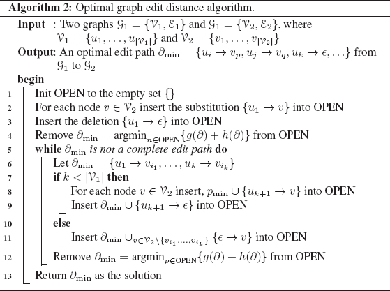
In Algorithm 2, the A*-based method for optimal graph edit distance computation is used. The nodes of the source graph $G_{1}$ are processed in the order (u₁, u₂,…). While there are unprocessed nodes of the first graph, substitutions (line 8) and insertions (line 9) of a node are considered. If all nodes of the first graph have been processed, the remaining nodes of the second graph are inserted in a single step (line 11). These three operations produce a number of successor nodes in the search tree. The set OPEN of partial edit paths contains the search tree nodes to be processed in the next steps. The most promising partial edit path ∂ ∈ OPEN, i.e., the one that minimizes g(∂)+h(∂), is always chosen first (lines 4 and 12). This procedure guarantees that the first complete edit path found by the algorithm is always optimal, i.e., has minimal costs among all possible competing paths (line 13).

Note that edit operations on edges are implied by edit operations on their adjacent nodes. Thus, insertions, deletions, and substitutions of edges depend on the edit operations performed on the adjacent nodes. Obviously, the implied edge operations can be derived from every partial or complete edit path during the search procedure given in Algorithm 2. The costs of these implied edge operations are dynamically added to the corresponding paths in OPEN.

The use of heuristics has been proposed in [77]. This allows one to integrate more knowledge about partial solutions in the search tree and possibly reduce the number of partial solutions that need to be evaluated to find the solution. The main objective in the introduction of heuristics is the estimation of a lower bound h(∂) on the future costs. The simplest scenario is to set this lower bound estimation h(∂) equal to zero for all ∂, which is equivalent to using no heuristic information about the present situation at all. On the other hand, the most complex scenario would be to perform a complete edit distance computation for each node of the search tree to a leaf node. It is easy to see, however, that in this case the function h(∂) is not a lower bound, but the exact value of the optimal costs. Of course, the computation of such a perfect heuristic is both unreasonable and intractable. Somewhere in between these two extremes, one can define a function h(∂) evaluating how many edit operations have to be performed in a complete edit path at least [69].

13.4.2 Suboptimal Algorithms

The method described so far finds an optimal edit path between two graphs. Unfortunately, regardless of the use of a heuristic function h(∂), the computational complexity of the edit distance algorithm is exponential in the number of nodes of the involved graphs. This restricts the applicability of the optimal algorithm since the running time and space complexity may be huge even for rather small graphs.

For this reason, a number of methods addressing the high computational complexity of graph edit distance computation have been proposed in recent years. One direction to tackle this problem and to make graph matching more efficient is to restrict considerations to special classes of graphs. Examples include the classes of planar graphs [24], bounded-valence graphs [23], trees [78], and graphs with unique node labels [34]. Another approach, which has been proposed recently [79], requires the nodes of graphs to be planarly embedded, which is satisfied in many computer vision applications of graph matching. Another approach is to perform a local search to solve the graph matching problem. The main idea is to optimize local criteria instead of global, or optimal, ones [80]. In [81], for instance, a linear programming method for computing the edit distance of graphs with unlabeled edges is proposed. The method can be used to derive lower and upper edit distance bounds in polynomial time. A number of graph matching methods based on genetic algorithms have been proposed [47]. Genetic algorithms offer an efficient way to cope with large search spaces, but are nondeterministic. In [82] a simple variant of an edit distance algorithm based on A* together with a heuristic is proposed. Instead of expanding all successor nodes in the search tree, only a fixed number s of nodes to be processed are kept in the OPEN set. Whenever a new partial edit path is added to OPEN in Algorithm 1, only the s partial edit paths ∂ with the lowest costs g(∂) + h(∂) are kept, and the remaining partial edit paths in OPEN are removed. Obviously, this procedure corresponds to a pruning of the search tree during the search procedure, i.e., not the full search space is explored, but only those nodes are expanded that belong to the most promising partial matches. Another approach to solve the problem of graph edit distance computation by means of bipartite graph matching is introduced in [83]. This approach will be explained in detail in the next section since we will use it in the last part of the chapter. In a recent approach [84], graph edit distance by means of an HMM-based approach is used to perform image indexing. For more information about the graph edit distance, the reader is referrer to a recent survey [85].

13.4.3 GED Computation by Means of Bipartite Graph Matching

In this approach the graph edit distance is approximated by finding an optimal match between nodes of two graphs together with their local structure. The computation of graph edit distance is actually reduced to the assignment problem.

The assignment problem considers the task of finding an optimal assignment of the elements of a set A to the elements of a set B, where A and B have the same cardinality. Assuming that numerical costs c are given for each assignment pair, an optimal assignment is one which minimizes the sum of the individual assignment costs. Usually, given two sets A and B with |A| = |B| = n, a cost matrix C ∈ M_nxn containing real numbers is defined. The matrix elements C_ij correspond to the costs of assigning the i-th element of A to the j-th element of B. The assignment problem is then reduced to find a permutation p = p₁, …, p_n of the integers 1, 2, …, n that minimizes $\sum_{i = 1}^{n} C_{i p_{i}}$ .

The assignment problem can be reformulated as finding an optimal matching in a complete bipartite graph and is therefore also referred to as the bipartite graph matching problem. Solving the assignment problem in a brute force manner by enumerating all permutations and selecting the one that minimizes the objective function leads to an exponential complexity which is unreasonable, of course. However, there exists an algorithm which is known as Munkres’ algorithm [86] that solves the bipartite matching problem in polynomial time. The assignment cost matrix C defined above is the input to the algorithm, and the output corresponds to the optimal permutation, i.e., the assignment pairs resulting in the minimum cost. In the worst case, the maximum number of operations needed by the algorithm is O(n³). Note that the O(n³) complexity is much smaller than the O(n!) complexity required by a brute force algorithm.

The assignment problem described above can be used to find the optimal correspondence between the nodes of one graph and the nodes of another graph. Let us assume that a source graph $G_{1} = {V_{1}, ℰ_{1}}$ and a target graph $G_{2} = {V_{2}, ℰ_{2}}$ of equal size are given. If we set $A = V_{1}$ and $B = V_{2}$ , then one can use Munkres’ algorithm in order to map the nodes of $V_{1}$ to the nodes of $V_{2}$ such that the resulting node substitution costs are minimal. In that approach the cost matrix C is defined such that the entry C_ij corresponds to the cost of substituting the i-th node of $V_{1}$ with the j-th node of $V_{2}$ . That is, C_ij = c(u_i → υ_j), where $u_{i} \in V_{1}$ and $υ_{j} \in V_{2}$ , for $i, j = 1, \dots, | V_{1} |$ .

Note that the above approach only allows the matching of graphs with the same number of nodes. Such a constraint is too restrictive in practice since it cannot be expected that all graphs in a specific problem domain always have the same number of nodes. However, this lack can be overcome by defining a quadratic cost matrix C which is more general in the sense that it allows insertions and/or deletions to occur in both graphs under consideration. Thus, given two graphs $G_{1} = {V_{1}, ℰ_{1}}$ and $G_{2} = {V_{2}, ℰ_{2}}$ with $V_{1} = {u_{1}, \dots, u_{m}}$ and $V_{2} = {υ_{1}, \dots, υ_{n}}$ and $| V_{1} |$ not necessarily being equal to $| V_{2} |$ , the new cost matrix C is defined as

$C = [\begin{array}{l} c_{1, 1} & c_{1, 2} & \dots & c_{1, m} & c_{1, ϵ} & \infty & \dots & \infty \\ c_{2, 1} & c_{2, 2} & \dots & c_{2, m} & \infty & c_{2, ϵ} & \dots & \infty \\ ⋮ & ⋮ & ⋱ & ⋮ & ⋮ & ⋱ & ⋱ & \infty \\ c_{n, 1} & c_{n, 2} & \dots & c_{n, m} & \infty & \infty & \dots & c_{n, ϵ} \\ c_{ϵ, 1} & \infty & \dots & \infty & 0 & 0 & 0 & 0 \\ \infty & c_{ϵ, 2} & \dots & \infty & 0 & 0 & ⋱ & ⋮ \\ ⋮ & ⋱ & ⋱ & \infty & ⋮ & ⋱ & ⋱ & 0 \\ \infty & \infty & \dots & c_{ϵ, m} & 0 & \dots & 0 & 0 \end{array}]$

(13.26)

where c_ϵj denotes the costs of a node insertion c(ϵ → υ_j), c_iϵ denotes the cost of a node deletion c(u_i → ϵ), and c_ij denotes the cost of a node substitution c(u_i → υ_j).

In the matrix C, the diagonal of the bottom left corner represents the costs of all possible node insertions. In the same way, the diagonal of the right upper corner represents the costs of all possible node deletions. Finally, the left upper corner of the cost matrix represents the costs of all possible node substitutions. Since each node can be deleted or inserted at most once, any nondiagonal element of the right-upper and left-lower part is set to ∞. The bottom right corner of the cost matrix is set to zero since substitutions of the form c(ϵ → ϵ) do not cause any costs.

Munkres’ algorithm [86] can be executed using the new cost matrix C as input. The algorithm finds the optimal permutation $h = h_{1}, \dots, h_{n + m}$ of the integers 1, 2, …, n + m that minimizes $\sum_{i = 1}^{n + m} C_{i h}$ , i.e., the minimum cost. Obviously, this is equivalent to the minimum cost assignment of the nodes of $G_{1}$ to the nodes of $G_{2}$ . Thus, the answer of the Munkres’ algorithm (each row and each column contains only one assignment), ensures that each node of graph $G_{1}$ is either uniquely assigned to a node of $G_{2}$ (substitution), or to the node ϵ (deletion). In the same way, each node of graph $G_{2}$ is either uniquely assigned to a node of $G_{1}$ (substitution), or to the node ϵ (insertion). The remaining e nodes corresponding to rows n + 1, …, n + m and columns m + 1, …, m + n in C that are not used cancel each other out without any costs.

Note that, up to now, only the nodes have been taken into account, and no information about the edges has been considered. This could lead to obtaining a poor approximation of the real cost of the optimal edit path. Therefore, in order to achieve a better approximation of the true edit distance, it is highly desirable to involve edge operations and their costs in the node assignment process as well. In order to achieve this goal, the authors propose an extension of the cost matrix [87]. Thus, to each entry c_{i, j} in the cost matrix C, i.e. to each node substitution c(u_i → v_j), the minimum sum of edge edit operation costs implied by the substitution is added. For instance, imagine that $ℰ_{u_{i}}$ denotes the set of edges adjacent to node u_i and $ℰ_{υ_{j}}$ denotes the set of edges adjacent to node υ_i. We can define a cost matrix D similarly to Equation (13.26) with the elements of $ℰ_{u_{i}}$ and $ℰ_{υ_{j}}$ . Then, applying the Munkres’ algorithm over this matrix D one can find the optimal assignment of the elements $ℰ_{u_{i}}$ to the elements of $ℰ_{υ_{j}}$ . Clearly, this procedure leads to the minimum sum of edge edit costs implied by the given node substitution u_i → υ_j. Then, these edge edit costs are added to the entry c_{i, j}. For deletions and insertions the procedure is slightly different. For the entries c_{i, ϵ}, which denote the cost of a node deletion, the cost of the deletion of all adjacent edges of u_i is added, and for the entries c_{ϵ, j}, which denote the cost of a node insertion, the cost of all insertions of the adjacent edges of υ_j is added.

Regardless of the improved handling of the edges, note that Munkres’ algorithm used in its original form is optimal for solving the assignment problem, but it provides us with a suboptimal solution for the graph edit distance problem only. This is due to the fact that each node edit operation is considered individually (considering the local structure only), such that no implied operations on the edges can be inferred dynamically. The result returned by Munkres’ algorithm corresponds to the minimum cost mapping, according to matrix C, of the nodes of $G_{1}$ to the nodes of $G_{2}$ . Given this mapping, the implied edit operations of the edges are inferred, and the accumulated costs of the individual edit operations on both nodes and edges can be computed. The approximate edit distance values obtained by this procedure are equal to, or larger than, the exact distance values, since the bipartite matching algorithm finds an optimal solution in a subspace of the complete search space. Although the method provides only approximate solutions to the graph edit distance, it has been shown that, in some cases, the provided results are very close to the optimal solutions [83]. This fact in conjunction with the polynomial time complexity makes this method particularly useful. In a recent paper [88], an even faster version of this method has been reported, where the assignment algorithm of Volgenant and Jonker [89] rather than the Munkres’ algorithm is used. An application of bipartite graph matching to approximately solving the graph isomorphism problem is described in [90].

13.5 Applications of GED

In this final part of the chapter we will show three applications where the graph edit distance is used. The first two applications, the weighted mean of a pair of graphs and the graph embedding into vector spaces, are general procedures that can be widely used in the context of other applications. An example of the general nature of weighted mean and graph embedding is the third application, the median graph computation, where the first two procedures are used to solve this hard problem approximately.

13.5.1 Weighted Mean of a Pair of Graphs

Consider two points in the n-dimensional real space, $x, y \in ℝ^{n}$ , where n ≥ 1. Their weighted mean can be defined as a point z such that

$z = γ x + (1 - γ) y, 0 \leq γ \leq 1$

(13.27)

Clearly, if $γ = \frac{1}{2}$ , then z is the (normal) mean of x and y. If z is defined according to Equation 13.27 then z − x = (1 − γ)(y − x) and y − z = (1 − γ)(y − x). In other words, z is a point on the line segment in n dimensions that connects x and y, and the distance between z and both x and y is controlled via the parameter γ.

In [91] the authors described the same concept but applied it to the domain of graphs, which resembles the weighted mean as described by Equation 13.27. Formally speaking, the weighted mean of a pair of graphs can be defined as follows.

Definition 13.5.1

Weighted mean: Let $G$ and $G^{'}$ be graphs with labels from the alphabet L. Let U be the set of graphs that can be constructed using labels from L and let

$I = {h \in U | d (G, G^{'}) = d (G, h) + d (h, G^{'})},$

be the set of intermediate graphs. Given $0 \leq a \leq d (G, G^{'})$ , the weighted mean of $G$ and $G^{'}$ is a graph

$g^{″} = W M (G, G^{'}, a) = \arg \min_{h \in I} | d (G, h) - a | .$

(13.28)

Intuitively, given two graphs, $G$ and $G^{'}$ , and a parameter a, the weighted mean is an intermediate graph, not necessarily unique, whose distance to $G$ is as similar as possible to a. Consequently, its distance to $G^{'}$ is also the closest to $d (G, G^{'}) - a$ . Again, although the definition is valid for any distance function, we let d be the graph edit distance. For this distance function, an efficient computation of the weighted mean is given in [91]. Figure 13.4 shows an example of the weighted mean of a pair of graphs where the distance is the graph edit distance.

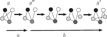
FIGURE 13.4
Example of the weighted mean of a pair of graphs. In this case a coincides with the cost of deletion of the edge between the white and the light grey nodes. Therefore, the graph $G^{″}$ is a weighted mean for which $| d (G, G^{″}) - a | = 0$ .

Note that the so called error, $ϵ (a) = | d (G, G^{″}) - a |$ , is not necessarily null. This fact, regardless of the exactness of the computation, depends on the properties of the search space U.

As a practical example of the use of the weighted mean, consider graph representations of drawings consisting of straight line segments. Figure 13.5(a) shows an example of these kind of drawings. In our representation, a node in the graph corresponds to an endpoint of a line segment or a point of intersection between two line segments, and edges represent lines that connect two adjacent intersections or end points which each other. The label of a node represents the location of that node in the image. There are no edge labels. Figure 13.5(b) shows an example of such a representation. The cost of the edit operations under this representation is as follows:

• Node insertion and deletion cost c(u → ϵ) = c(ϵ → u) = β₁

• Node substitution cost $c (u, υ) = c ((u_{1}, u_{2}), (υ_{1}, υ_{2})) = \sqrt{{(u_{1} - υ_{1})}^{2} + {(u_{2} - υ_{2})}^{2}}$

• Cost of deleting or inserting an edge e is c(e → ϵ) = c(ϵ → e) = β₂

The cost of a node substitution is equal to the Euclidean distance of the locations of the two considered nodes in the image, while the cost of node deletions and insertions, as well as edge deletions and insertions, are user defined constants, β₁ and β₂. As there are no edge labels, no edge substitutions need to be considered. Figure 13.6 shows an example of the result of applying the weighted mean of two graphs with different values of a.

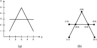
FIGURE 13.5
Example of graph-based representation.

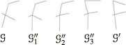
FIGURE 13.6
Example of the weighted mean of a pair of graphs. $G$ and $G^{'}$ represent the original graphs while the intermediate graphs ${G^{″}}_{1}$ to ${G^{″}}_{3}$ represents graphs obtained with different values of a.

From the domain of line drawing analysis, a number of practical examples of weighted mean graph were given in the literature. These examples demonstrate that weighted mean is a useful concept to synthesize patterns $G^{″}$ that have certain degrees of similarity to given patterns $G$ and $G^{'}$ . In the examples the intuitive notion of shape similarity occurs to correspond well with the formal concept of graph edit distance.

13.5.2 Graph Embedding into Vector Spaces

Graph embedding [92] aims at converting graphs into real vectors, and then operate in the associated space to make easier some typical graph-based tasks, such as matching and clustering [93, 94]. To this end, different graph embedding procedures have been proposed in the literature. Some of them are based on spectral graph theory. Others take advantage of typical similarity measures to perform the embedding task. For instance, a relatively early approach based on the adjacency matrix of a graph is proposed in [53]. In this work, graphs are converted into a vector representation using some spectral features extracted from the adjacency matrix of a graph. Then, these vectors are embedded into eigenspaces with the use of the eigenvectors of the covariance matrix of the vectors. This approach is then used to perform graph clustering. Another approach has been presented in [95]. This work is similar to the previous one, but in this case the authors use the coefficients of some symmetric polynomials, constructed from the spectral features of the Laplacian matrix, to represent the graphs in a vectorial form. Finally, in a recent approach [96], the idea is to embed the nodes of a graph into a metric space and view the graph edge set as geodesics between pairs of points on a Riemannian manifold. Then, the problem of matching the nodes of a pair of graphs is viewed as the alignment of the embedded point sets. In this section we will describe a new class of graph embedding procedures based on the selection of some prototypes and graph edit distance computation. The basic intuition of this work is that the description of regularities in the observation of classes and objects is the basis to perform pattern classification. Thus, based on the selection of concrete prototypes, each point is embedded into a vector space by taking its distance to all these prototypes. Assuming these prototypes have been chosen appropriately, each class will form a compact zone in the vector space.

General Embedding Procedure Using Dissimilarities

The idea of this graph embedding framework [87] stems from the seminal work done by Duin and Pekalska [97] where dissimilarities for pattern representation are used for the first time. Later, this method was extended so as to map string representations into vector spaces [98]. The following approach further extends and generalizes methods described in [97, 98] to the domain of graphs. The key idea of this approach is to use the distances of an input graph to a number of training graphs, termed prototype graphs, as a vectorial description of the graph. That is, we use the dissimilarity representation for pattern recognition rather than the original graph based representation.

Assume we have a set of training graphs $T = {G_{1}, G_{2}, \dots, G_{n}}$ and a graph dissimilarity measure $d (G_{i}, G_{j}) (i, j = 1 \dots n; G_{i}, G_{j} \in T)$ . Then, a set Ω = {ρ₁, …, ρ_m} ⊆ T of m prototypes is selected from T (with m ≤ n). After that, the dissimilarity between a given graph of $G \in T$ and every prototype ρ ∈ Ω is computed. This leads to m dissimilarity values, d₁, …, d_m where $d_{k} = d (G, ρ_{k})$ . These dissimilarities can be arranged in a vector (d₁, …, d_m). In this way, we can transform any graph of the training set T into an m-dimensional vector using the prototype set P. More formally this embedding procedure can be defined as follows:

Definition 13.5.2

Graph embedding: Given a set of training graphs $T = {G_{1}, G_{2}, \dots G_{n}}$ and a set of prototypes Ω = {ρ₁, …, ρ_m} ⊆ T, the graph embedding

$ψ : T \to ℝ^{m}$

(13.29)

is defined as the function

$ψ (G) \to (d (G, p_{1}), d (G, ρ_{2}), \dots, d (G, ρ_{m}))$

(13.30)

where $G \in T$ , and $d (G, ρ_{i})$ is a graph dissimilarity measure between the graph $G$ and the i-th prototype ρ_i.

Obviously, by means of this definition a vector space is obtained where each axis is associated with a prototype graph ρ_i ∈ Ω. The coordinate values of an embedded graph $G$ are the distances of $G$ to the elements in P. In this way one can transform any graph $G$ from the training set T as well as any other graph set S (for instance, a validation or a test set of a classification problem), into a vector of real numbers. In other words, the graph set to be embedded can be arbitrarily extended. Training graphs which have been selected as prototypes before have a zero entry in their corresponding graph map. Although any dissimilarity measure can be employed to embed the graphs, the graph edit distance has been used to perform graph classification with very good results in [87].

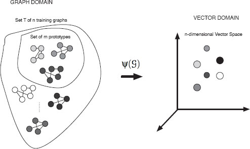
FIGURE 13.7
Overview of graph embedding.

13.5.3 Median Graph Computation

In some machine learning algorithms a representative of a set of objects is needed. For instance, in the classical k-means clustering algorithm, a representative of each cluster is computed and used at the next iteration to reorganize the clusters. In classification tasks using the k-nearest neighbour classifier, a representative of a class could be useful to reduce the number of comparisons needed to assign the unknown input pattern to its closest class. While the computation of a representative of a set is a relatively simple task in the vector domain (it can be computed by means of the mean or the median vector), it is not clear how to obtain a representative of a set of graphs. One of the proposed solutions to this problem is the median graph.

In this section we present a novel approach to the computation of the median graph that is faster and more accurate than previous approximate algorithms. It is based on the graph embedding procedure presented in the last section.

Introduction to the Median Graph Problem

The generalized median graph has been proposed to represent a set of graphs.

Definition 13.5.3

Median Graph: Let U be the set of graphs that can be constructed using labels from L. Given $S = {G_{1}, G_{2}, \dots, G_{n}} \subseteq U$ , the generalized median graph $\bar{G}$ of S is defined as:

$\bar{G} = \underset{G \in U}{\arg \min} \sum_{G_{i} \in S} d (G, G_{i})$

(13.31)

That is, the generalized median graph $\bar{G}$ of S is a graph $G \in U$ that minimizes the sum of distances (SOD) to all the graphs in S. Notice that $\bar{G}$ is usually not a member of S, and in general more than one generalized median graph may exist for a given set S. Graph $\bar{G}$ can be seen as a representative of the set. Consequently, it can be potentially used by any graph-based algorithm where a representative of a set of graphs in needed, for example, in graph-based clustering.

However, the computation of the median graph is extremely complex. As implied by Equation (13.31), a distance measure $d (G, G_{i})$ between the candidate median $G$ and every graph $G_{i} \in S$ must be computed. Therefore, since the computation of the graph distance is a well-known NP-complete problem, the computation of the generalized median graph can only be done in exponential time, both in the number of graphs in S and their size (even in the special case of strings, the time required is exponential in the number of input strings [99]). As a consequence, in real applications we are forced to use suboptimal methods in order to obtain approximate solutions for the generalized median graph in reasonable time. Such approximate methods [100, 101, 102, 103] apply some heuristics in order to reduce the complexity of the graph distance computation and the size of the search space. Recent works [104, 105] rely on graph embedding in vector spaces.

Computation via Embedding

Given a set $S = {G_{1}, G_{2}, \dots, G_{n}}$ of n graphs, the first step is to embed every graph of S into the n-dimensional space of real numbers, i.e., each graph becomes a point in $ℝ^{n}$ (Figure 13.7). The second step consists in computing the median using the vectors obtained in the previous step. Finally, we go from the vector space back to the graph domain, converting the median vector into a graph. The resulting graph is taken as the median graph of S. These three steps are depicted in Figure 13.8. In the following subsections, these three main steps will be further explained.

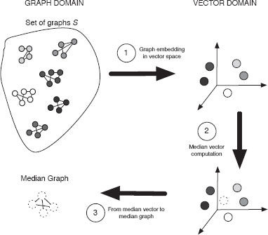
FIGURE 13.8
Overview of the approximate procedure for median graph computation.

• Step I. Graph Embedding in Vector Space: The embedding procedure we use in this paper follows the procedure proposed in [106] (Section 13.5.2) but we let the training set T and the prototype set P be the same, i.e, the set S for which the median graph is to be computed. So, we compute the graph edit distance between every pair of graphs in set S. These distances are arranged in a distance matrix. Each row or column of the matrix can be seen as an n-dimensional vector. Since each row and column of the distance matrix is assigned to one graph, such an n-dimensional vector is the vectorial representation of the corresponding graph (Figure 13.9).

• Step II. Computation of the Median Vector: Once all graphs have been embedded in the vector space, the median vector is computed. To this end we use the concept of Euclidean median.

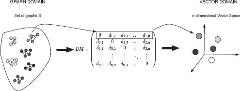
FIGURE 13.9
Step I. Graph embedding.

Definition 13.5.4

Euclidean median: Given a set X = {x₁, x₂, …, x_m} of m points with $x_{i} \in ℝ^{n}$ for i = 1 …m, the geometric median is defined as

$Euclidean median = \underset{y \in ℝ^{n}}{\arg \min} \sum_{i = 1}^{m} ‖ x_{i} - y ‖$

where ||x_i – y|| denotes the Euclidean distance between the points $x_{i}, y \in ℝ^{n}$ .

That is, the Euclidean median is a point $y \in ℝ^{n}$ that minimizes the sum of the Euclidean distances between itself and all the points in X. It corresponds with the definition of the median graph, but in the vector domain. The Euclidean median cannot be calculated in a straightforward way. The exact location of the Euclidean median can not always be found when the number of elements in X is greater than 5 [107]. No algorithm in polynomial time is known, nor has the problem been shown to be NP-hard [108]. In this work, we will use the most common approximate algorithm for the computation of the Euclidean median, which is the Weiszfeld’s algorithm [109]. It is an iterative procedure that converges to the Euclidean median. To this end, the algorithm first chooses an initial estimate solution y (this initial solution is often chosen randomly). Then, the algorithm defines a set of weights that are inversely proportional to the distances from the current estimate to the samples, and creates a new estimate that is the weighted average of the samples according to these weights. The algorithm may finish either when a predefined number of iterations is reached, or under some other criteria, for instance, when the difference between the current estimate and the previous one is less than a threshold.

• Step III. Back to Graph Domain: This step is similar to the so called preimage problem in spectral analysis where one wants to go back from the spectral to the original domain. In our particular case, the last step in median graph computation is to transform the Euclidean median into a graph. Such a graph will be considered as an approximation of the median graph of the set S. To this end we will use a triangulation procedure based on the weighted mean of a pair of graphs [91] and the edit path between two given graphs.

This triangulation procedure, illustrated in Figure 13.10, works as follows. Given the n-dimensional points representing every graph in S (the white dots in Figure 13.10(a)), and the Euclidean Median vector υ_m (the grey dot in Figure 13.10(a)), we first select the three closest points to the Euclidean median (υ₁ to υ₃ in Figure 13.10(a)). Notice that we know the corresponding graph of each of these points (in Figure 13.10(a) we have indicated this fact by labelling them with the pair υ_j, $G_{j}$ with j = 1 … 3). Then, we compute the median vector ${υ^{'}}_{m}$ of these three points (represented as a black dot in Figure 13.10(a)). Notice that ${υ^{'}}_{m}$ is in the plane formed by υ₁, υ₂ and υ₃. With υ₁ to υ₃ and ${υ^{'}}_{m}$ at hand (Figure 13.10(b)), we arbitrarily choose two out of these three points (without loss of generality we can assume that we select υ₁ and υ₂), and we project the remaining point (υ₃) onto the line joining υ₁ and υ₂. In this way, we obtain a point υ_i in between υ₁ and υ₂ (Figure 13.10(c)). With this point at hand, we can compute the percentage of the distance in between υ₁ and υ₂ where υ_i is located (Figure 13.10(d)). As we know the corresponding graphs of the points υ₁ and υ₂ we can obtain the graph $G_{i}$ corresponding to υ_i by applying the weighted mean procedure (Figure 13.10(e)). Once $G_{i}$ is known, we can obtain the percentage of distance in between υ_i and υ₃ where ${υ^{'}}_{m}$ is located and obtain ${G^{'}}_{m}$ applying again the weighted mean procedure (Figure 13.10(f)). Finally, ${G^{'}}_{m}$ is chosen as the approximation for the generalized median of the set S.

Discussion of the Approximations

The proposed approximate embedding procedure is composed of three steps: the graph embedding into a vector space, the median vector computation and the return to the graph domain. Each of these steps introduces some kind of approximation to the final solution. In the first step, in order to deal with large graphs, an approximate edit distance algorithm is normally used. Thus, each vector representing a graph includes small errors in its coordinates with respect to the optimal distance between two graphs. Nevertheless, the two approximate methods we used for the edit distance computation [82, 83] provide correlation scatter plots showing a high accuracy with respect the exact distance computation. Also, the median vector computation introduces a certain amount of error, since the Weiszfeld method obtains approximations for the median vector. This factor may lead to choosing three points that might not be the best points to go back to the graph domain. In addition, small errors may be introduced when choosing ${υ^{'}}_{m}$ instead of υ_m to obtain the weighted mean of a pair of graphs. Finally, when the weighted mean between two points is computed, the graph edit path is composed of a set of discrete steps, each having its own cost. When returning to the graph domain, the percentage of distance needed to obtain the weighted mean of a pair of graphs may fall in between two of these edit operations. Since we choose only one of them, small errors may also be introduced in this step. Despite of these possible errors, the proposed method has shown very good results and compares favourably to competing algorithms [105].

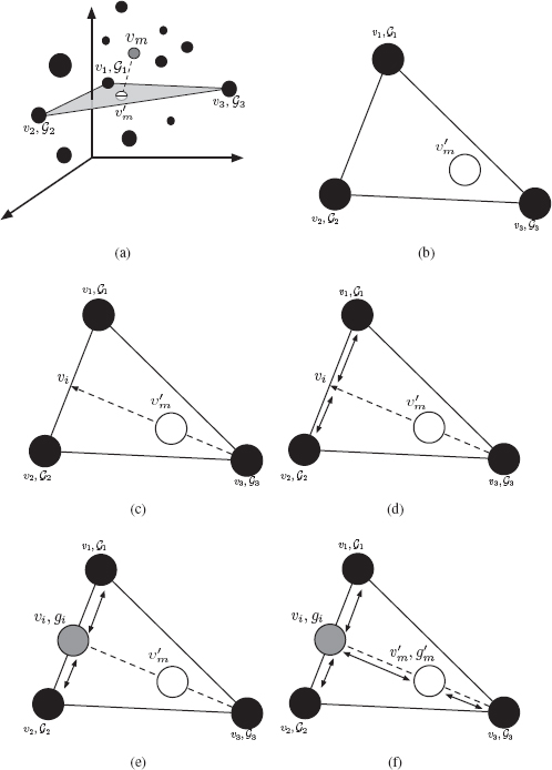
FIGURE 13.10
Illustration of the triangulation procedure.

13.6 Conclusions

In this chapter we have reviewed the graph edit distance (GED) from three points of view. It is a method that is recognized as one of the most flexible and universal approaches to error-tolerant graph matching. In the first part of the chapter, we introduced fundamental concepts related to GED, such as graph similarity to finally introduce the concept of graph edit distance. Then we focused on the theory underlying the graph edit distance, putting special emphasis on the cost function, giving some examples, and introducing the fundamental problem of automatic edit cost learning. In the second part of the chapter we gave an introduction to GED computation. We reviewed in detail exact and approximate methods for GED computation. We finished this second part by introducing one of the most recent approximate algorithms for GED computation, which is based on bipartite graph matching. Finally, the last part of the chapter is devoted to GED applications. We concentrated on three basic applications: the weighted mean of a pair of graphs, graph embedding into vector spaces, and the median graph computation problem. All of them demonstrate that graph edit distance is a truly versatile and flexible similarity measure that is potentially beneficial to various fields where graph representations are being used.

Bibliography

[1] R. Duda, P. Hart, and D. Stork, Pattern Classification. Wiley Interscience. 2nd Edition, 2000.

[2] M. Friedman and A. Kandel, Introduction to Pattern Recognition. World Scientific, 1999.

[3] L. da F. Costa, F. A. Rodrigues, G. Travieso, and P. V. Boas, “Characterization of complex networks: A survey of measurements,” Advances in Physics, vol. 56, no. 1, pp. 167–242, 2007.

[4] L. Grady and J. R. Polimeni, Discrete Calculus: Applied Analysis on Graphs for Computational Science. Springer, 2010.

[5] A. Schenker, H. Bunke, M. Last, and A. Kandel, Graph-Theoretic Techniques for Web Content Mining. River Edge, NJ: World Scientific Publishing Co., Inc., 2005.

[6] S. Lee, J. Kim, and F. Groen, “Translation-, rotation-, and scale invariant recognition of hand-drawn symbols in schematic diagrams,” International Journal of Pattern Recognition and Artificial Intelligence, vol. 4, pp. 1–15, 1990.

[7] J. Lladós, E. Martí, and J. J. Villanueva, “Symbol recognition by error-tolerant subgraph matching between region adjacency graphs,” IEEE Trans. Pattern Anal. Mach. Intell., vol. 23, no. 10, pp. 1137–1143, 2001.

[8] S. W. Lu, Y. Ren, and C. Y. Suen, “Hierarchical attributed graph representation and recognition of handwritten chinese characters,” Pattern Recognition, vol. 24, no. 7, pp. 617–632, 1991.

[9] J. Rocha and T. Pavlidis, “A shape analysis model with applications to a character recognition system,” IEEE Trans. Pattern Anal. Mach. Intell., vol. 16, no. 4, pp. 393–404, 1994.

[10] V. Cantoni, L. Cinque, C. Guerra, S. Levialdi, and L. Lombardi, “2-D object recognition by multiscale tree matching,” Pattern Recognition, vol. 31, no. 10, pp. 1443–1454, 1998.

[11] M. Pelillo, K. Siddiqi, and S. W. Zucker, “Matching hierarchical structures using association graphs,” IEEE Trans. Pattern Anal. Mach. Intell., vol. 21, no. 11, pp. 1105–1120, 1999.

[12] F. Serratosa, R. Alquézar, and A. Sanfeliu, “Function-described graphs for modelling objects represented by sets of attributed graphs,” Pattern Recognition, vol. 36, no. 3, pp. 781–798, 2003.

[13] E. K. Wong, “Model matching in robot vision by subgraph isomorphism,” Pattern Recognition, vol. 25, no. 3, pp. 287–303, 1992.

[14] K. Shearer, H. Bunke, and S. Venkatesh, “Video indexing and similarity retrieval by largest common subgraph detection using decision trees,” Pattern Recognition, vol. 34, no. 5, pp. 1075–1091, 2001.

[15] J. R. Ullman, “An algorithm for subgraph isomorphism,” Journal of ACM, vol. 23, no. 1, pp. 31–42, Jan. 1976.

[16] J. J. McGregor, “Backtrack search algorithms and the maximal common subgraph problem,” Software - Practice and Experience, vol. 12, no. 1, pp. 23–24, 1982.

[17] H. Bunke, X. Jiang, and A. Kandel, “On the minimum common supergraph of two graphs,” Computing, vol. 65, no. 1, pp. 13–25, 2000.

[18] D. C. Schmidt and L. E. Druffel, “A fast backtracking algorithm to test directed graphs for isomorphism using distance matrices,” J. ACM, vol. 23, no. 3, pp. 433–445, 1976.

[19] L. P. Cordella, P. Foggia, C. Sansone, and M. Vento, “Fast graph matching for detecting cad image components,” in 15th International Conference on Pattern Recognition, 2000, pp. 6034–6037.

[20] C. S. L.P. Cordella, P. Foggia and M. Vento, “An improved algorithm for matching large graphs,” in Proc. 3rd IAPR Workshop Graph-Based Representations in Pattern Recognition, 2001, pp. 149–159.

[21] P. Fosser, R. Glantz, M. Locatelli, and M. Pelillo, “Swap strategies for graph matching,” in GbRPR, ser. Lecture Notes in Computer Science, E. R. Hancock and M. Vento, Eds., vol. 2726. Springer, 2003, pp. 142–153.

[22] B. McKay, “Practical graph isomorphism,” Congressus Numerantum, vol. 30, pp. 45–87, 1981.

[23] E. Luks, “Isomorphism of graphs of bounded valence can be tested in polynomial time,” Journal of Computer and System Sciences, vol. 25, pp. 42–65, 1982.

[24] J. E. Hopcroft and J. K. Wong, “Linear time algorithm for isomorphism of planar graphs (preliminary report),” in STOC ’74: Proceedings of the sixth annual ACM symposium on Theory of computing. New York: ACM Press, 1974, pp. 172–184.

[25] M. R. Garey and D. S. Johnson, Computers and Intractability: A Guide to the Theory of NP-Completeness. New York: W. H. Freeman & Co., 1979.

[26] E. B. Krissinel and K. Henrick, “Common subgraph isomorphism detection by backtracking search,” Softw., Pract. Exper., vol. 34, no. 6, pp. 591–607, 2004.

[27] Y. Wang and C. Maple, “A novel efficient algorithm for determining maximum common subgraphs,” in 9th International Conference on Information Visualisation, IV 2005, 6–8 July 2005, London, UK. IEEE Computer Society, 2005, pp. 657–663.

[28] E. Balas and C. S. Yu, “Finding a maximum clique in an arbitrary graph,” SIAM J. Comput., vol. 15, no. 4, pp. 1054–1068, 1986.

[29] P. J. Durand, R. Pasari, J. W. Baker, and C. che Tsai, “An efficient algorithm for similarity analysis of molecules,” Internet Journal of Chemistry, vol. 2, no. 17, 1999.

[30] C. Bron and J. Kerbosch, “Finding all the cliques in an undirected graph,” Communication of the ACM, vol. 16, pp. 189–201, 1973.

[31] H. Bunke, P. Foggia, C. Guidobaldi, C. Sansone, and M. Vento, “A comparison of algorithms for maximum common subgraph on randomly connected graphs,” in Structural, Syntactic, and Statistical Pattern Recognition, Joint IAPR International Workshops SSPR 2002 and SPR 2002, Windsor, Ontario, Canada, August 6–9, 2002, Proceedings. Lecture Notes in Computer Science Vol. 2396, 2002, pp. 123–132.

[32] D. Conte, P. Foggia, and M. Vento, “Challenging complexity of maximum common subgraph detection algorithms: A performance analysis of three algorithms on a wide database of graphs,” Journal of Graph Algorithms and Applications, vol. 11, no. 1, pp. 99–143, 2007.

[33] I. M. Bomze, M. Budunuch., P. M. Paralos, and M. Pelillo, The Maximum Clique Problem. Dordrecht: Kluwer Academic Publisher, 1999.

[34] P. J. Dickinson, H. Bunke, A. Dadej, and M. Kraetzl, “Matching graphs with unique node labels,” Pattern Anal. Appl., vol. 7, no. 3, pp. 243–254, 2004.

[35] J. W. Raymond and P. Willett, “Maximum common subgraph isomorphism algorithms for the matching of chemical structures,” Journal of Computer-Aided Molecular Design, vol. 16, no. 7, pp. 521–533, 2002.

[36] Y. Takahashi, Y. Satoh, H. Suzuki, and S. Sasaki, “Recognition of largest common structural fragment among a variety of chemical structures,” Analytical Sciences, vol. 3, no. 1, pp. 23–28, 1987.

[37] H. Y. Sumio Masuda and E. Tanaka, “Algorithm for finding one of the largest common subgraphs of two three-dimensional graph structures,” Electronics and Communications in Japan (Part III: Fundamental Electronic Science), vol. 81, no. 9, pp. 48–53, 1998.

[38] H. Bunke, “On a relation between graph edit distance and maximum common subgraph,” Pattern Recognition Letters, vol. 18, no. 8, pp. 689–694, 1997.

[39] H. Bunke and K. Shearer, “A graph distance metric based on the maximal common subgraph,” Pattern Recognition Letters, vol. 19, no. 3–4, pp. 255–259, 1998.

[40] W. D. Wallis, P. Shoubridge, M. Kraetz, and D. Ray, “Graph distances using graph union,” Pattern Recognition Letters, vol. 22, no. 6/7, pp. 701–704, 2001.

[41] M.-L. Fernández and G. Valiente, “A graph distance metric combining maximum common subgraph and minimum common supergraph,” Pattern Recognition Letters, vol. 22, no. 6/7, pp. 753–758, 2001.

[42] A. Dumay, R. van der Geest, J. Gerbrands, E. Jansen, and J. Reiber, “Consistent inexact graph matching applied to labelling coronary segments in arteriograms,” in 11th International Confenrence on Pattern Recognition, 1992, pp. III: 439–442.

[43] S. Berretti, A. D. Bimbo, and E. Vicario, “Efficient matching and indexing of graph models in content-based retrieval,” IEEE Trans. Pattern Anal. Mach. Intell., vol. 23, no. 10, pp. 1089–1105, 2001.

[44] F. Serratosa, R. Alquezar, and A. Sanfeliu, “Function-described graphs: a fast algorithm to compute a sub-optimal matching measure,” in Proceedings of the 2nd IAPR-TC15 Workshop on Graph-based Representations in Pattern Recognition, 1999, pp. 71–77.

[45] R. Allen, L. Cinque, S. L. Tanimoto, L. G. Shapiro, and D. Yasuda, “A parallel algorithm for graph matching and its maspar implementation,” IEEE Trans. Parallel Distrib. Syst., vol. 8, no. 5, pp. 490–501, 1997.

[46] S. Auwatanamongkol, “Inexact graph matching using a genetic algorithm for image recognition,” Pattern Recognition Letters, vol. 28, no. 12, pp. 1428–1437, 2007.

[47] A. D. J. Cross, R. C. Wilson, and E. R. Hancock, “Inexact graph matching using genetic search,” Pattern Recognition, vol. 30, no. 6, pp. 953–970, 1997.

[48] M. Singh, A. Chatterjee, and S. Chaudhury, “Matching structural shape descriptions using genetic algorithms,” Pattern Recognition, vol. 30, no. 9, pp. 1451–1462, September 1997.

[49] P. N. Suganthan, “Structural pattern recognition using genetic algorithms,” Pattern Recognition, vol. 35, no. 9, pp. 1883–1893, 2002.

[50] Y.-K. Wang, K.-C. Fan, and J.-T. Horng, “Genetic-based search for error-correcting graph isomorphism,” IEEE Transactions on Systems, Man, and Cybernetics, Part B, vol. 27, no. 4, pp. 588–597, 1997.

[51] K. A. D. Jong and W. M. Spears, “Using genetic algorithms to solve NP-complete problems,” in ICGA, J. D. Schaffer, Ed. Morgan Kaufmann, 1989, pp. 124–132.

[52] T. Caelli and S. Kosinov, “An eigenspace projection clustering method for inexact graph matching,” IEEE Trans. Pattern Anal. Mach. Intell., vol. 26, no. 4, pp. 515–519, 2004.

[53] B. Luo, R. C. Wilson, and E. R. Hancock, “Spectral embedding of graphs,” Pattern Recognition, vol. 36, no. 10, pp. 2213–2230, 2003.

[54] A. Robles-Kelly and E. R. Hancock, “Graph edit distance from spectral seriation,” IEEE Trans. Pattern Anal. Mach. Intell., vol. 27, no. 3, pp. 365–378, 2005.

[55] A. Shokoufandeh, D. Macrini, S. J. Dickinson, K. Siddiqi, and S. W. Zucker, “Indexing hierarchical structures using graph spectra,” IEEE Trans. Pattern Anal. Mach. Intell., vol. 27, no. 7, pp. 1125–1140, 2005.

[56] S. Umeyama, “An eigendecomposition approach to weighted graph matching problems,” IEEE Transactions on Pattern Analysis and Machine Intelligence, vol. 10, no. 5, pp. 695–703, September 1988.

[57] R. C. Wilson and E. R. Hancock, “Levenshtein distance for graph spectral features,” in 17th Internarional Conference on Pattern Recognition, 2004, pp. 489–492.

[58] L. Xu and I. King, “A PCA approach for fast retrieval of structural patterns in attributed graphs,” IEEE Transactions on Systems, Man and Cybernetics - Part B, vol. 31, no. 5, pp. 812–817, October 2001.

[59] M. Carcassoni and E. R. Hancock, “Weighted graph-matching using modal clusters,” in CAIP ’01: Proceedings of the 9th International Conference on Computer Analysis of Images and Patterns. London, UK: Springer-Verlag, 2001, pp. 142–151.

[60] S. Kosinov and T. Caelli, “Inexact multisubgraph matching using graph eigenspace and clustering models,” in Structural, Syntactic, and Statistical Pattern Recognition, Joint IAPR International Workshops SSPR 2002 and SPR 2002, Windsor, Ontario, Canada, August 6–9, 2002, Proceedings. Lecture Notes in Computer Science Vol. 2396, 2002, pp. 133–142.

[61] A. Shokoufandeh and S. J. Dickinson, “A unified framework for indexing and matching hierarchical shape structures,” in IWVF, ser. Lecture Notes in Computer Science, C. Arcelli, L. P. Cordella, and G. S. di Baja, Eds., vol. 2059. Springer, 2001, pp. 67–84.

[62] W.-J. Lee, R. P. W. Duin, and H. Bunke, “Selecting structural base classifiers for graph-based multiple classifier systems,” in MCS, ser. Lecture Notes in Computer Science, N. E. Gayar, J. Kittler, and F. Roli, Eds., vol. 5997. Springer, 2010, pp. 155–164.

[63] W. J. Christmas, J. Kittler, and M. Petrou, “Structural matching in computer vision using probabilistic relaxation,” IEEE Trans. Pattern Anal. Mach. Intell., vol. 17, no. 8, pp. 749–764, 1995.

[64] R. C. Wilson and E. R. Hancock, “Structural matching by discrete relaxation,” IEEE Trans. Pattern Anal. Mach. Intell., vol. 19, no. 6, pp. 634–648, 1997.

[65] B. Luo and E. R. Hancock, “Structural graph matching using the EM algorithm and singular value decomposition,” IEEE Trans. Pattern Anal. Mach. Intell., vol. 23, no. 10, pp. 1120–1136, 2001.

[66] A. P. Dempster, N. M. Laird, and D. B. Rubin, “Maximum likelihood from incomplete data via the EM algorithm,” Journal of the Royal Statistical Society, vol. 39, no. 1, pp. 1–38, 1977. [Online]. Available: http://links.jstor.org/sici?sici=0035-9246\%281977\%2939\%3A1\%3C1\%3AMLFIDV\%3E2.0.CO\%3B2-Z

[67] S. Gold and A. Rangarajan, “A graduated assignment algorithm for graph matching,” IEEE Trans. Pattern Anal. Mach. Intell., vol. 18, no. 4, pp. 377–388, 1996.

[68] D. Conte, P. Foggia, C. Sansone, and M. Vento, “Thirty years of graph matching in pattern recognition,” International Journal of Pattern Recognition and Artificial Intelligence, vol. 18, no. 3, pp. 265–298, 2004.

[69] H. Bunke and G. Allerman, “Inexact graph matching for structural pattern recognition,” Pattern Recognition Letters, vol. 1, no. 4, pp. 245–253, 1983.

[70] M. A. Eshera and K. S. Fu, “A graph distance measure for image analysis,” IEEE Transactions on Systems, Man and Cybernetics, vol. 14, pp. 398–408, 1984.

[71] A. Sanfeliu and K. Fu, “A distance measure between attributed relational graphs for pattern recognition,” IEEE Transactions on Systems, Man and Cybernetics, vol. 13, no. 3, pp. 353–362, May 1983.

[72] W. H. Tsai and K. S. Fu, “Error-correcting isomorphisms of attributed relational graphs for pattern analysis,” IEEE Transactions on Systems, Man and Cybernetics, vol. 9, pp. 757–768, 1979.

[73] M. Neuhaus and H. Bunke, “Automatic learning of cost functions for graph edit distance,” Inf. Sci., vol. 177, no. 1, pp. 239–247, 2007.

[74] E. S. Ristad and P. N. Yianilos, “Learning string-edit distance,” IEEE Trans. Pattern Anal. Mach. Intell., vol. 20, no. 5, pp. 522–532, 1998.

[75] T. Kohonen, Self-Organizing Maps. Berlin: Springer, 1995.

[76] M. Neuhaus and H. Bunke, “Self-organizing maps for learning the edit costs in graph matching,” IEEE Transactions on Systems, Man, and Cybernetics, Part B, vol. 35, no. 3, pp. 503–514, 2005.

[77] P. E. Hart, N. J. Nilsson, and B. Raphael, “A formal basis for the heuristic determination of minimum costs paths,” IEEE Transactions of Systems, Science, and Cybernetics, vol. 4, no. 2, pp. 100–107, 1968.

[78] A. Torsello, D. H. Rowe, and M. Pelillo, “Polynomial-time metrics for attributed trees,” IEEE Trans. Pattern Anal. Mach. Intell., vol. 27, no. 7, pp. 1087–1099, 2005.

[79] M. Neuhaus and H. Bunke, “An error-tolerant approximate matching algorithm for attributed planar graphs and its application to fingerprint classification,” in SSPR/SPR, ser. Lecture Notes in Computer Science, A. L. N. Fred, T. Caelli, R. P. W. Duin, A. C. Campilho, and D. de Ridder, Eds., vol. 3138. Springer, 2004, pp. 180–189.

[80] M. C. Boeres, C. C. Ribeiro, and I. Bloch, “A randomized heuristic for scene recognition by graph matching,” in WEA, ser. Lecture Notes in Computer Science, C. C. Ribeiro and S. L. Martins, Eds., vol. 3059. Springer, 2004, pp. 100–113.

[81] D. Justice and A. O. Hero, “A binary linear programming formulation of the graph edit distance,” IEEE Trans. Pattern Anal. Mach. Intell., vol. 28, no. 8, pp. 1200–1214, 2006.

[82] M. Neuhaus, K. Riesen, and H. Bunke, “Fast suboptimal algorithms for the computation of graph edit distance,” in Joint IAPR International Workshops, SSPR and SPR 2006. Lecture Notes in Computer Science 4109, 2006, pp. 163–172.

[83] K. Riesen and H. Bunke, “Approximate graph edit distance computation by means of bipartite graph matching,” Image and Vision Computing, vol. 27, no. 7, pp. 950–959, 2009.

[84] B. Xiao, X. Gao, D. Tao, and X. Li, “HMM-based graph edit distance for image indexing,” International Journal of Imaging Systems and Technology - Multimedia Information Retrieval, vol. 8, no. 2-3, pp. 209–218, 2008.

[85] X. Gao, B. Xiao, D. Tao, and X. Li, “A survey of graph edit distance,” Pattern Analysis and Applications, vol. 13, pp. 113–129, 2010.

[86] J. Munkres, “Algorithms for the assignment and transportation problems,” Journal of the Society of Industrial and Applied Mathematics, vol. 5, no. 1, pp. 32–38, March 1957.

[87] K. Riesen and H. Bunke, Graph Classification and Clustering Based on Vector Space Embedding. World Scientific, 2010.

[88] S. Fankhauser, K. Riesen, and H. Bunke, “Speeding up graph edit distance computation through fast bipartite matching,” in GbRPR, ser. Lecture Notes in Computer Science, X. Jiang, M. Ferrer, and A. Torsello, Eds., vol. 6658. Springer, 2011, pp. 102–111.

[89] R. Jonker and T. Volgenant, “A shortest augmenting path algorithm for dense and sparse linear assignment problems,” Computing, vol. 38, pp. 325–340, 1987.

[90] K. Riesen, S. Fankhauser, H. Bunke, and P. J. Dickinson, “Efficient suboptimal graph isomorphism,” in GbRPR, ser. Lecture Notes in Computer Science, A. Torsello, F. Escolano, and L. Brun, Eds., vol. 5534. Springer, 2009, pp. 124–133.

[91] H. Bunke and S. Günter, “Weighted mean of a pair of graphs,” Computing, vol. 67, no. 3, pp. 209–224, 2001.

[92] P. Indyk, “Algorithmic applications of low-distortion geometric embeddings,” in IEEE Symposium on Foundations of Computer Science, 2001, pp. 10–33.

[93] K. Grauman and T. Darrell, “Fast contour matching using approximate earth mover’s distance,” in Proceedings of the 2004 IEEE Computer Society Conference on Computer Vision and Pattern Recognition, 2004, pp. 220–227.

[94] M. F. Demirci, A. Shokoufandeh, Y. Keselman, L. Bretzner, and S. J. Dickinson, “Object recognition as many-to-many feature matching,” International Journal of Computer Vision, vol. 69, no. 2, pp. 203–222, 2006.

[95] R. C. Wilson, E. R. Hancock, and B. Luo, “Pattern vectors from algebraic graph theory,” IEEE Trans. Pattern Anal. Mach. Intell., vol. 27, no. 7, pp. 1112–1124, 2005.

[96] A. Robles-Kelly and E. R. Hancock, “A Riemannian approach to graph embedding,” Pattern Recognition, vol. 40, no. 3, pp. 1042–1056, 2007.

[97] E. Pekalska and R. Duin, The Dissimilarity Representation for Pattern Recognition - Foundations and Applications. World Scientific, 2005.

[98] B. Spillmann, M. Neuhaus, H. Bunke, E. Pekalska, and R. P. W. Duin, “Transforming strings to vector spaces using prototype selection,” in Structural, Syntactic, and Statistical Pattern Recognition, Joint IAPR International Workshops, SSPR 2006 and SPR 2006, Hong Kong, China, August 17-19, 2006, Proceedings, 2006, pp. 287–296.

[99] C. de la Higuera and F. Casacuberta, “Topology of strings: Median string is NP-complete,” Theor. Comput. Sci., vol. 230, no. 1-2, pp. 39–48, 2000.

[100] M. Ferrer, F. Serratosa, and A. Sanfeliu, “Synthesis of median spectral graph,” in Second Iberian Conference of Pattern Recognition and Image Analysis. Volume 3523 LNCS, 2005, pp. 139–146.

[101] A. Hlaoui and S. Wang, “Median graph computation for graph clustering,” Soft Comput., vol. 10, no. 1, pp. 47–53, 2006.

[102] X. Jiang, A. Münger, and H. Bunke, “On median graphs: Properties, algorithms, and applications,” IEEE Trans. Pattern Anal. Mach. Intell., vol. 23, no. 10, pp. 1144–1151, 2001.

[103] D. White and R. C. Wilson, “Mixing spectral representations of graphs,” in 18th International Conference on Pattern Recognition (ICPR 2006), 20-24 August 2006, Hong Kong, China. IEEE Computer Society, 2006, pp. 140–144.

[104] M. Ferrer, E. Valveny, F. Serratosa, I. Bardají, and H. Bunke, “Graph-based k-means clustering: A comparison of the set median versus the generalized median graph,” in CAIP, ser. Lecture Notes in Computer Science, X. Jiang and N. Petkov, Eds., vol. 5702. Springer, 2009, pp. 342–350.

[105] M. Ferrer, E. Valveny, F. Serratosa, K. Riesen, and H. Bunke, “Generalized median graph computation by means of graph embedding in vector spaces,” Pattern Recognition, vol. 43, no. 4, pp. 1642–1655, 2010.

[106] K. Riesen, M. Neuhaus, and H. Bunke, “Graph embedding in vector spaces by means of prototype selection,” in 6th IAPR-TC-15 International Workshop, GbRPR 2007, ser. Lecture Notes in Computer Science, vol. 4538. Springer, 2007, pp. 383–393.

[107] C. Bajaj, “The algebraic degree of geometric optimization problems,” Discrete Comput. Geom., vol. 3, no. 2, pp. 177–191, 1988.

[108] S. L. Hakimi, Location Theory. CRC Press., 2000.

[109] E. Weiszfeld, “Sur le point pour lequel la somme des distances de n points donnés est minimum,” Tohoku Math. Journal, no. 43, pp. 355–386, 1937.

1 As it is straightforward to transform a similarity measure into a dissimilarity measure and vice versa, we use the term similarity and dissimilarity interchangeably in this chapter.

2 We defined the graph matching process as simply the way to ontain a similarity measure between graphs. However, one can see the graph matching a richer process where more valuable information, such as the mapping between nodes and edges can be obtained.

3 Unless otherwise stated, in this work we will suppose graphs with directed edges.

..................Content has been hidden....................

You can't read the all page of ebook, please click here login for view all page.

Table of Contents for 13 Graph Edit Distance—Theory, Algorithms, and Applications

Create new playlist

Sign In

Sign Up

Table of Contents for
13 Graph Edit Distance—Theory, Algorithms, and Applications