16 Modeling Images with Undirected Graphical Models

As computer vision and image processing systems become more complex, it is increasingly important to build models in a way that makes it possible to manage this complexity. This chapter will discuss mathematical models of images that can be represented with graphs, known as graphical models. These models are powerful because graphs provide an powerful mechanism for describing and understanding the structure of the models. This chapter will review how these models are typically defined and used in computer vision systems.

16.2 Background

One of the first steps in creating a computer vision system is the establishment of the overall computational paradigm that will be used to compute the final solution. One of the most common and flexible ways to implement a solution is through the combination of an energy function and MAP inference.

The term MAP inference is an acronym for Maximum A Posteriori inference and has its roots in probabilistic estimation theory. For the purposes of the discussion here, the MAP inference strategy begins with the definition of a probability distribution p(x|y)¹, where x is the vector of random variables being estimated from the observations y. In MAP inference, the actual estimate x* is found by finding the vector x* that maximizes p(x|y). This is sometimes referred to as a point estimate because the estimate is limited to a single point, as opposed to actually calculating the posterior distribution p(x|y).

The connection with energy functions can be seen by expressing p(x|y) as a Gibbs distribution:

$p (x | y) = \frac{1}{Z} \exp (- \sum_{C} E_{C} (x_{C}; y))$

(16.1)

where $E_{C} (x_{C}; y)$ denotes an energy function over a set of elements of x. This makes the sum in Equation 16.1 a sum over different sets of elements of x. The structure of these sets is vital to the construction of the model and will be discussed in Section 16.2.3.1. The constant Z is a normalization constant that ensures that p(x|y) is a valid probability distribution.

With this representation, it can be seen that MAP inference is equivalent to finding the vector x* that maximizes the energy function

$E (x; y) = \sum_{C} E_{C} (x_{C}; y) .$

(16.2)

It should be noted that this focus on MAP inference should not be construed as minimizing the usefulness of computing the full posterior distribution over possible values of x. However, computing the MAP estimate is often much easier because it is only necessary to compute a single point.

16.2.1 Designing the Energy Function—The Need for Graphical Models

A key motivation in designing graphical models can be seen by considering an example image enhancement problem. In this motivating problem, imagine the goal is to estimate a high-quality image, denoted x, from a corrupted observation, denoted y. This basic formulation encompasses a number of different, challenging problems, including deblurring, denoising, and super-resolution.

Assuming that a MAP estimation strategy will be employed, the next step is to decide on the form of the distribution p(x|y). Assuming that, for simplicity, x represents a 2 × 2 image, with 256 possible states, corresponding to gray-levels, per pixel. For this type of random vector, specifying just p(x), and ignoring the relationships with the observation y, would require 256⁴ values to be determined if p(x) was specified in its simplest tabular form. The huge number of values is necessary because the model must account for every interaction between the four pixels.

Now consider a simplification of this model where only some interactions are considered. The model can be simplified if only the interactions between horizontal and vertical neighbors are considered. Using the labeling shown in Figure 16.1(a), only the interactions between A-B, A-C, C-D, and B-D would be modeled. Again, using a simple tabular specification of the interactions between the states at different pixels requires 256² values to be specified, leading to 4(256²) required values to specify the distribution, which is 16384 times fewer values. Far fewer parameters are necessary because this new model ignored diagonal interactions between pairs of nodes and interactions between sets of three and four nodes. This reduction is possible because interactions between nodes like A and D are not modeled explicitly, but are handled by combination of interactions between the A − − B and B − − D interactions, among others. It should be remembered that this is just for a 2×2 image; the reduction in complexity grows quickly as the image becomes larger.

Of course, this simplified model is only useful if the resulting estimate x* is comparable to the result from the complete model. That is the key challenge in designing a model for image processing and analysis: finding the simplest model that performs the desired task well. Graphical models have proved to be a very useful tool because they make it possible to control the complexity of the model by controlling the complexity of the interactions between the variables being estimated.

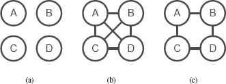
FIGURE 16.1
Each of these graphs represents the pixels in a simple 2 × 2 image. Each pixel is represented by a node in the graph. The edges in the graph represent how the relationships between pixels are expressed in different models. The graph in (a) describes a model that does not consider interrelationships between pixels, while the graph in (c) denotes a model that could simultaneously consider the relationship between all pixels. The graph in (b) describes a model that is more descriptive than (a), but simpler than (c). This model is built on the relationships between neighboring pixels.

16.2.2 Graph Representations of Distributions

Graphical models are sonamed because the distribution can be represented with a graph. Each variable is represented by a node in the graph, so the 2 × 2 image from the previous section can be represented by the four nodes in Figure 16.1(a). For now, the edges can be informally described as representing interactions that are explicitly described in the model. (A more formal definition will follow.) The completely specified model can then be represented with the connected graph shown in Figure 16.1 (b). In this graph, there are edges between every pair of nodes because the interaction between every pair of nodes is modeled explicitly.

In contrast, the graph for the simplified model, where only the relationship between neighboring horizontal and vertical neighbors is explicitly modeled, is shown in Figure 16.1(c). Notice that the diagonal edges are missing, indicating that the relationship between these nodes is not explicitly modeled. Of course, this does not mean that the values of at nodes A and D do not affect each other when performing inference. As mentioned earlier, the model in Figure 16.1(c) indicates that they do interact, but only indirectly through the interactions between B and C. If the value at A is constrained by the model to be similar to the value at B, which is likewise constrained to be similar to the value at D, then A will be indirectly constrained to be similar to D.

16.2.3 Formally Specifying a Graphical Model

An intrinsic characteristic of a graphical model is that the graph representation is explicitly connected to the mathematical specification of a model. The graph, like Figure 16.1 describes the factorization of the distribution. The distribution over values of x, again temporarily ignoring y, for the graph in Figure 16.1(c) has the form

$p (x) = \frac{1}{Z} ψ_{1} (x_{A}, x_{B}) ψ_{2} (x_{A}, x_{C}) ψ_{3} (x_{B}, x_{D}) ψ_{4} (x_{C}, x_{D})$

(16.3)

$= \frac{1}{Z} \exp [- (E_{1} (x_{A}, x_{B}) + E_{2} (x_{A}, x_{C}) + E_{3} (x_{B}, x_{D}) + E_{4} (x_{C}, x_{D}))]$

(16.4)

Here, we have shown the distribution as both the product of a set of potential functions, ψ(·) and as a Gibbs distribution with energy functions, E₁(·),…, E₄(·).

For comparison, the distribution for the model where all joint relationships are modeled would simply be²

$\begin{array}{l} p (x) & = \frac{1}{Z} ψ_{1} (x_{A}, x_{B}, x_{C}, x_{D}) \\ = \frac{1}{Z} \exp [- E (x_{A}, x_{B}, x_{C}, x_{D})] . \end{array}$

(16.5)

Notice that no factorization is possible in this model because the model must have an individual energy value for every possible joint set of values.

The factorization in Equation (16.3) expresses the distribution over the whole vector x through a set of local relationships between neighboring pixels. This is advantageous for both specifying the model and for performing inference. This factorization is valuable because it makes it possible to construct a global model over pixels in an image by combining local relationships between pixels. It will likely be easier to construct appropriate potentials for neighboring pixels than to construct a single potential that captures all of the relationships between many different pixels. As will be discussed later, this factorization into local relationships also often makes inference more computationally efficient.

16.2.3.1 General Specifications of Graphical Models

Graphical models like the model in Equation (16.5) are referred to as undirected graphical models because they can be represented with an undirected graph³.

The undirected graphical model is described by the potential functions ψ(·), which are functions of subsets of nodes in the graph. The nodes included in any particular potential function correspond to a clique in the graph, which is a subset of nodes where there is an edge between each pair of nodes in the clique. Each potential in a graphical model is a function of one of these cliques.

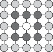
FIGURE 16.2
This graph demonstrates how the graph describing a graphical model can be analyzed to determine conditional independence relationships. The node at the center, colored in white, is conditionally independent of the light gray nodes, conditioned on the dark gray nodes. Intuitively, these relationships imply that once the values of the dark gray nodes are known, the light gray nodes provide no more information about what values the white node should take.

If $x_{C}$ denotes a clique in the graph, then the corresponding distribution can be defined as

$p (x) = \frac{1}{Z} \prod_{C} ψ_{C} (x_{C}),$

(16.6)

where the product is over all cliques $C$ . In this equation, the term 1/Z is a normalization constant and is often referred to as the partition function. This product form can also be expressed in terms of energy functions, similar to Equation (16.1), by calculating the logarithm of the potentials.

Typically, the cliques $C$ are maximal cliques, which are essentially the largest possible cliques. If a clique is a maximal clique, then if any node is added the subset will no longer be a clique. The maximal clique representation can also represent any model based on nonmaximal cliques, as the maximal clique would subsume the potential functions based on nonmaximal cliques.

16.2.4 Conditional Independence

In addition to describing how the model is factorized, the graph representing a graphical model can also be analyzed to find conditional independence relationships in the model. Any node in the model is independent of all other nodes, conditioned on the nodes connected to it. Thus, in a lattice model, like the model shown in Figure 16.2, the node at the center, colored in white, is independent of the nodes colored in light gray, when conditioned on the nodes colored in dark gray. The nodes shown in dark gray can be called the Markov blanket. Intuitively, these relationships imply that once the values of the dark gray nodes are known, the light gray nodes provide no more information about what values the white node should take.

Returning to the four node graph in Figure 16.1, these conditional independence statements can be written formally in statements like

$p (x_{A} | x_{B}, x_{C}, x_{D}) = p (x_{A} | x_{B}, x_{C})$

(16.7)

$p (x_{A}, x_{D} | x_{B}, x_{C}, x_{D}) = p (x_{A} | x_{B}, x_{C}) p (x_{D} | x_{B}, x_{C})$

(16.8)

These conditional independence relationships between nodes in the graph and variables in the vector have led these models to also be commonly called Markov Random Fields.

16.2.5 Factor Graphs

A weakness of the graph representation discussed so far is that it can be ambiguous. Consider the fully connected undirected graphical model in Figure 16.3(a). This graph could represent a number of different factorizations, including

$p (x) = \frac{1}{Z} ψ_{1} (x_{A}, x_{B}, x_{D}) ψ_{2} (x_{A}, x_{C}, X_{D})$

(16.9)

$p (x) = \frac{1}{Z} ψ_{1} (x_{A}, x_{C}, x_{D}) ψ_{2} (x_{A}, x_{B}) ψ_{3} (x_{B}, x_{D})$

(16.10)

The factor graph representation removes this ambiguity by representing the model with a bipartite graph, with nodes explicitly representing the potentials [2]. In a factor graph, each potential is represented with a node. As variables are often represented with unfilled circles, the factors are usually represented with solid black squares. Figure 16.3(b) shows the factor graph representation of the model in Equation (16.9). In this representation, edges connect the node representing each potential to the nodes that interact in that potential.

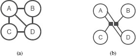
FIGURE 16.3
The graph in (a) represents the model in Equation (16.9) with the same graph that would represent a model with a different factorization. Figure (b) shows a factor graph representation that uses a bipartite graph to explicitly represent different potentials.

16.3 Graphical Models for Modeling Image Patches

Undirected graphical models are a natural tool for modeling patches of pixels in low-level image models. A good example of a patch-based models is the model used for super-resolution in [3]. In this model, a graphical model is used to estimate a high-resolution image from a low-resolution observation, y.

In patch-based models, the image is divided into square patches, with one node in the model per patch. These patches are typically chosen by examining the observed image y. In the model from [3], Freeman et al. use the observed low-resolution image to search a database for high-resolution patches that have a similar appearance when the resolution is reduced to match the observation. The patches can also be created dynamically, as in [4].

The system’s estimate, x*, is created by mosaicing together the patches chosen at each node. One of the advantages of a patch-based model is that it makes it possible to model an image with a discrete-valued graphical model. A discrete-valued graphical model may be useful if it is desirable to arbitrarily specify the relationship between patches because the potentials can be expressed in a tabular form. Some of the most powerful inference algorithms discussed in Section 16.5 are also designed for graphical models.

The graph in patch-based models is typically structured as a pairwise lattice, similar to the model shown in Figure 16.2. In this model, all of the cliques consist of horizontal or vertical neighbors. In [3], the potential functions are specified by examining the overlapping regions created by making the patches slightly larger than the patches that will be mosaiced together, as shown in Figure 16.4. This overlap region can then be used to create a potential function, which can be thought of as a compatibility function that measures how compatible the possible choices of patches at two neighboring nodes are. In [3], the compatibility function measured by computing the squared difference between the two patches in the overlap region, as illustrated in Figure 16.4. Formally, this can be expressed as

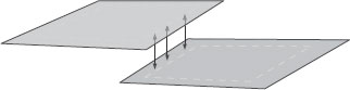
FIGURE 16.4
This figure illustrates one strategy for computing the compatibility between neighboring image patches. The resulting image will be created from mosaicing together the interior outlined regions. The compatibility between patches is measured by examining the overlapping regions outside of the outlined areas.

$ψ (x_{p}, x_{q}) = \exp (- \sum_{i \in O} {(t_{i}^{x_{p}} - t_{i}^{x_{q}})}^{2})$

(16.11)

where $t_{i}^{x_{p}}$ refers to the value of the ith pixel in the patch that would be used if node p took the value x_p. This sum is computed over the overlapping region $O$ .

The basic function of this potential is that patches that are very similar in the overlap region will be considered compatible. Similar models have been used for other applications, such as editing photographs [5] or synthesizing texture [6]. The work in [6] further extends these models by allowing the use of nonsquare image patches.

16.4 Pixel-Based Graphical Models

The most common alternative to patches in image models is to directly model pixels. Directly modeling pixels is particularly common in stereo and image enhancement applications, where a graphical model can be used to express priors based on smoothness.

16.4.1 Stereopsis

The most difficult problem in stereopsis is correctly matching the pixels between two views of the scene, particularly when a pixel in one image matches with multiple pixels in the other image equally well. If multiple pixels match equally well, then other assumptions must be used to disambiguate the problem. A common assumption is that the surface is smooth. This transforms the stereopsis problem into the task of finding matches where matched pixels are both similar visually and lead to a reconstruction with smooth surfaces.

Undirected graphical models have a long history of application to this task. In many cases, the purpose of the model is also described in terms of regularizing the solution [7, 8]. One of the most common formulations of the stereo problem is through an energy function on a vector containing one variable per pixel in the graph. Each variable typically represents the disparity between the location of the pixel in the reference image and the location of the matching pixel in the other image. A common form of the energy function is

$E (x) = E_{Data} (x; y) + E_{Smooth} (x)$

(16.12)

where E_Data(x; y) and E_Smooth(x) are energy functions representing the visual similarity and smoothness of the surfaces, respectively [9, 10].

The term E_Data(x; y) measures the visual similarity between pixels matched by the disparity values in x. This energy function is often referred to as the data term because it captures the information in the data presented to the system. It is typically based on intensity differences in the observation y. Models for a number of different applications use a data term that captures the information in the observed data.

Because of the discretely sampled nature of images, the data term for stereo models is usually most easily expressed as a discrete-valued function, making the vector x a vector of discrete-valued variables. This has the added advantage of making it possible to use powerful inference techniques that will be discussed in Section 16.5.

The smoothness assumption is expressed in E_Smooth(x). Although the smoothness term is also usually discrete-valued, to be compatible with the data term, it is typically based on the difference between the disparities represented. Assuming that each element of x, x_i, is defined such that x_i ∈ {0,…, N − 1}, a basic smoothness term just measures the squared difference in disparity between neighboring pixels or

$E_{Smooth} (x) = \sum_{< p, q >} {(x_{p} - x_{q})}^{2} .$

(16.13)

In this formula, the sum is over all pairs of neighboring nodes, p and q. This is denoted in Equation (16.13) as < p, q >.

Equation (16.13) can be rewritten more generally with a penalty function ρ(·)

$E_{Smooth} (x) = \sum_{< p, q >} ρ (x_{p} - x_{q}) .$

(16.14)

where ρ(z) = z².

When designing a smoothness term, both the type of difference, such as first- or second-order difference, to use and the type of penalty function must be decided. The type of derivative influences the resulting shape. The first derivative, as in Equation (16.13), selects surfaces that are composed of fronto-parallel planes. If second-derivatives are used, the surface encouraged to be planar, but not necessarily fronto-parallel.

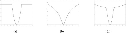
FIGURE 16.5
This figure shows three different types of potentials. The advantage of these potentials is that they combine the behavior of the quadratic and Potts models. Small differences are treated smoothly, while large differences have roughly the same penalty. This helps produce sharp edges in the results produced by the system.

The other key decision is the type of penalty function. The squared-error function used in Equation (16.13) is rarely used because this type of smoothness prior is known to lead to surfaces with blurry edges. As discussed in [4], a squared error criterion prefers smaller differences across several pixels instead of a large difference at one location. The effect of this is especially noticeable at the edges of objects. Rather than having a crisp, sharp edge where an object ends, a squared error criterion will lead to blurry edges that smoothly transition to the disparity levels of different objects.

The solution to this problem is to use different potentials for implementing the smoothness prior. For discrete-valued models, a popular potential is the Potts model, which is often expressed as an energy function as

$ρ_{Potts} (z) = {\begin{array}{l} 0 & if z = 0 \\ T & otherwise \end{array},$

(16.15)

where T is a constant chosen when the model is implemented.

The basic idea behind the Potts model is that neighboring pixels are encouraged to have the same disparity, but a fixed cost is assigned when they do not. The unique aspect of the Potts model is that the cost is the same no matter how great the difference in disparity. This is useful because there is typically no prior information about how separated objects should be; thus the same cost should be assigned to any change in disparity. The Potts model can also be thought of as using an L₀ norm to enforce sparsity in the horizontal and vertical gradients of the surface.

Other useful potentials can be seen as a balance of the quadratic penalty and Potts model. Figure 16.5(a) shows the truncated quadratic potential. This model allows for smooth variations in the surface by penalizing small changes in disparity with a quadratic model, but large changes in disparity behave as a Potts model. The truncated quadratic model can be expressed similarly to the Potts model:

$ρ_{TruncQuad} (z) = {\begin{array}{l} z^{2} & if | z < T | \\ T^{2} & otherwise \end{array},$

(16.16)

where T is a threshold determined when the model is constructed.

The truncated quadratic model works well if the model is discrete-valued. In that case, it can be used as a replacement for the Potts model. However, it may not be well suited for continuous-valued models. As will be discussed in Section 16.5, inference in continuous-valued models is often implemented with gradient-based optimization. The truncated quadratic model may be awkward if gradient-based optimization is used because it is discontinuous at the point when the difference between x_p and x_q exceeds T.

This problem can be avoided by using a potential that is continuous everywhere and is similar in shape to the truncated quadratic. Figures 16.5(b) and (c) show two examples of alternative potentials. Figure 16.5(b) shows the Lorentzian potential [11], which has the form

$ρ_{Lorentz} (z) = \log (1 + \frac{1}{2} z^{2})$

(16.17)

The Lorentzian potential is useful because the rate of increase of the penalty function decreases as the difference between x_p and x_q increases. In effect, when the difference between x_p and x_q is large, increases in this difference cause relatively small increases in the penalty function. This is similar to the Potts model in that once the change in disparity is large enough, the size of the disparity change has a relatively small impact on the energy of the smoothness term.

A more flexible term is based on Gaussian Scale Mixtures [12, 13]. A Gaussian scale mixture is a mixture model where the mean of each component is zero, but the variance changes. Figure 16.5(c) shows an example of a potential based on a two-component mixture. If the energy function is not constrained to be a true Gaussian mixture, then a potential like that shown in Figure 16.5(c) can be expressed as

$ρ_{GSM} (z) = - \log (\exp (- z^{2} / σ_{1} + T_{1}) + \exp (- z^{2} / σ_{2} + T_{2})),$

(16.18)

where T₁ and T₂ are constants.

The Gaussian Scale Mixture is particularly useful because multiple terms can be added to the sum in Equation (16.18). This makes it possible for the potentials to flexibly express many different shapes of potentials.

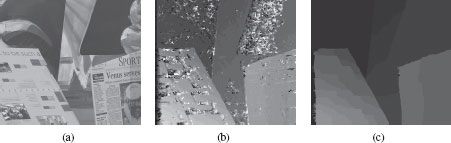
FIGURE 16.6
A stereo example that shows the benefit of the using a graphical model to estimate stereo disparity. (a) One input image from the stereo pair. An algorithm based on matching just using local windows will have difficulty in areas with little texture. (b) The disparity map recovered by matching using only local windows. Notice the noise in the disparity map in textureless areas of the scene. In these areas, the local texture is not sufficient to match. (c) This image shows the disparity map when a smoothness term is incorporated into overall cost function. Notice how the smoothness term eliminates noise in areas of low texture.

In addition to these potentials where the rate of change in the penalty decreases, the L1 penalty is also commonly used. This penalty is defined as

$ρ_{L1} (x_{p}, x_{q}) = | z | .$

(16.19)

16.4.1.1 Benefit of MRF Model for Stereo

The usefulness of a graphical model for estimating disparity in stereo image pairs can be seen in the example shown in Figure 16.6. Figure 16.6(b) shows the disparity map that would be recovered from the scene shown in Figure 16.6(a) using just the data term. Notice that in areas with little variation in texture, the disparity estimates are quite noisy.

As described above, this noise can be ameliorated by incorporating a smoothness term. In areas with low amounts of texture, the smoothness term effectively propagates information from areas with enough texture to make matching based on the data term possible. Without strong information from local matching, the smoothness term will cause the estimated disparity values to be smooth with respect to values in areas with good texture information. Figure 16.6(c) shows the disparity map recovered when a smoothness cost is incorporated. With the smoothness term added, the noise is eliminated.

16.4.2 Modeling Pixels in Natural Images

Popular models of images have much in common with the smoothness priors for stereopsis. A popular recent model is the Field of Experts model proposed by Roth and Black [14]. The model functions as a prior on images and is combined with a data term to produce estimates. This model is based on a set of filters, f₁,…, f_{N_f}, and weights, w₁,…, w_{N_f}, that are combined with a Lorentzian penalty to form

$E_{FoE} (x) = \sum_{p} \sum_{i = 1}^{N_{f}} - w_{i} \log (f_{i} * x_{p}),$

(16.20)

where the sum is over all pixels p. In this equation x_p denotes a patch of image centered at pixel p, which is the same size as the filter f_i. This makes the result of f_i ∗ x_p a scalar. While the form based on energy functions is shown here, the product form of this distribution is composed of a product of factors created from the Student’s t distribution.

Similar models have also been used in [15, 13]. This model can be justified in two different ways. The first justification is based on statistical properties of images. The histogram of the response of applying a filter to images has a characteristic shape. Figure 16.7(b) shows the histogram of a derivative filter applied to the image in Figure 16.7. The notable aspect of this shape is that it is sharply peaked around zero, and the tails of the distribution have more mass than would be seen in a Gaussian distribution. This type of distribution is referred to as a heavy-tailed distribution. As shown in Figure 16.7(c), the negative logarithm of this distribution has a similar shape as the Lorentzian penalty. The filters in the Field of Experts model that perform the best are larger than simple derivative filters used to generate the example in Figure 16.7, but the histogram of the response has a similar shape. Thus, the Field of Experts model can be thought of as modeling the marginal statistics of images. Improved versions of the model have also been produced by using Gaussian Scale Mixtures [13, 16].

Interestingly, the optimal filters for the Field of Experts model are similar to derivative filters. The Field of Experts model can also be viewed through the lens of smoothness, similar to the smoothness priors used in stereopsis. The Lorentzian penalty has a similar behavior as the truncated quadratic model, where small changes are penalized relative to the size of the change, but large changes have roughly the same penalty, which is not very dependent on the size of the change. This model can be seen as describing images as being made of smooth regions, with occasional large changes at edges. Because the filters used in the Field of Experts model are higher-order filters, the smoothness does not lead to flat regions in the image, but instead leads to smooth gradients.

Combined with a data term, this model has been applied to other tasks, such as in-painting [14].

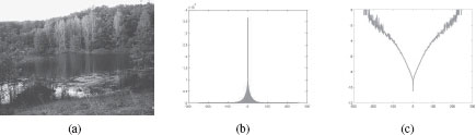
FIGURE 16.7
The structure of Field of Experts model, which is built around derivative-like filters, can be motivated by examining the statistics of natural images, such as the image shown in (a). Figure (b) shows the histogram of pixel values in the image created by filtering the image in (a) with a discrete-derivative filter. Figure (c) shows the log of the histogram in (b). The shape of this histogram is very similar to the shape of the potential functions used in the Field of Experts model. [Photo credit: Axel D from Flickr].

16.4.3 Incorporating Observations

Up this point, the issue of incorporating the observations has not been considered. At a high level, observations are typically implemented in a model in one of two ways. One approach is to model the joint distribution between the observations and the variables being estimated. In [3], the terms expressing the relationship between the observation and the hidden variables being estimated are denoted as ϕ(·) instead of ψ(·). This gives a pairwise lattice model, similar to Figure 16.2, of the form

$p (x, y) = \frac{1}{Z} \prod_{p} ϕ (x_{p}, y_{p}) \prod_{< p, q >} ψ (x_{p}, x_{q}),$

(16.21)

where the first product is over all pixels p and the second product is over all neighboring pairs of pixels.

Another approach is to simply make all of the factors in the distribution dependent on the observations. This is currently the most common approach because it offers the most flexibility. Models that do this are often called Conditional Random Field models or CRFs [17].

16.4.4 Beyond Modeling Images

While the focus of the previous sections have been on low-level vision models that model pixels, they have also been used to model parts in object, as in the pictorial structures model [18, 19]. In these models, the nodes in the graph represent the location of different parts. These models can be fit as generic shapes, as in [19], or can be fit to specific shape, such as the human form [20].

16.5 Inference in Graphical Models

After the model has been designed, MAP inference can be applied to recover the estimate x*. While graphical models offer a convenient tool for building models, there are still significant issues in finding x*. Inference in graphical models is an active, mathematically rigorous area of research, so this chapter will briefly survey popular approaches. More in-depth information and explanations can be found in [21, 1] and the original literature cited below. Szeliski et al. have also published a useful comparison of different inference techniques [22].

In some cases, the inference can be implemented in polynomial time using existing algorithms. If the energy function is the sum of convex quadratic terms, then the minimum energy solution x*, which corresponds to the MAP estimate, can be found by solving the linear system created by differentiating the energy function. Similarly, if the energy function can be expressed as the sum of absolute value penalties, then x* can be found with linear programming.

For more general continuous-valued models, the inference can be implemented with general optimization techniques, so it may not be possible to guarantee that the estimate of x* is the global optimum, rather than just a local optimum.

16.5.1 Inference in General, Tree-Structured Graphs

If the graph representation of the model does not have loops, then x* can be recovered using a simple iterative procedure known as Belief Propagation [23] or the max-product algorithm.

To see how this algorithm is derived, consider a simple three-node model

$p (x) = \frac{1}{Z} ψ (x_{1}, x_{2}) ψ (x_{2}, x_{3})$

(16.22)

In MAP inference, the goal is to compute

$x * = \arg \max_{x_{1}, x_{2}, x_{3}} ψ (x_{1}, x_{2}) ψ (x_{2}, x_{3}) .$

(16.23)

In this model, the joint max operation can be factored to make the computation more efficient:

$x * = \arg \max_{x_{2}} [\arg \max_{x_{1}} ψ (x_{1}, x_{2})] [\arg \max_{x_{3}} ψ (x_{2}, x_{3})]$

(16.24)

$= \max_{x_{2}} m_{1 \to 2} (x_{2}) m_{3 \to 2} (x_{2}) .$

(16.25)

In Equation (16.25), the max operations have been represented as message functions. Because the max functions on the right are over x₁ and x₃, these max operations generate functions of x₂. In Equation (16.25), these functions are represented as message functions that are passed from nodes x₁ and x₃ to x₂. The leftmost max function in Equation (16.23) computes the optimal label for x₂. The optimal labels for x₁ and x₃ can be computed by messages passed from x₂.

It can be shown that a similar message-passing routine can be used to perform MAP inference in graphs where there are no loops [21, 23]. In the general operation, inference is implemented through a series of message-passing operations.

The algorithm is easiest to describe for a pairwise graph, where all cliques are pairs of nodes. For a node, x_i in the graph, inference is implemented by a series of message-passing operations between x_i and the set of its neighbors, denoted as the set $N (x_{i})$ . At each iteration, the node x_i sends a message to each of its neighbors. The message from x_i to a neighbor x_j, denoted at m_i→j(x_j) is computed as

$m_{i \to j} (x_{j}) = \max_{x_{i}} ψ (x_{i}, x_{j}) \prod_{k \in N (x_{i}) j} m_{k \to i} (x_{i}),$

(16.26)

where $k \in N (x_{i}) j$ denotes all nodes k, besides j that are neighbors of x_i.

The optimal value of x_i is computed from the messages received by its neighbors,

$x_{i}^{*} = \arg \max \prod_{k \in N (x_{i})} m_{k \to i} (x_{i})$

(16.27)

For more complicated graphs, the factor graph representation is particularly useful [2].

16.5.2 Belief Propagation for Approximate Inference in Graphs with Loops

In graphs with loops, these steps do not lead to the optimal result because the messages sent out from a node eventually loop back to that node. However, research and practice has shown that applying the belief propagation algorithm on graphs with loops will still often produce good results [24, 25].

In general, the inference in graphs with loops is an NP-Complete inference problem [10, 1]. However, recent research has also introduced other message-passing algorithms that perform better at finding good approximate solutions. In particular, the Tree Re-Weighted Belief Propagation Algorithm, or TRW algorithm, proposed by Wainwright et al. [26] and the TRW-S improvements proposed by Kolmogorov [27] performed well in the comparisons in [22].

16.5.3 Graph-Cut Inference

An alternative to the message-passing algorithms for inference is the graph-cut approach proposed by Boykov et al. in [10].

This algorithm is based on the ability to find the MAP solution for certain binaryvalued graphical models by computing the min-cut of a graph [28]. While the min-cut can only be used to optimize a binary-valued graphical model, Boykov et al. introduced the α–expansion approach that uses this graph-cut procedure to compute an approximate solution. In the alpha expansion procedure, the optimization process is implemented as a series of expansion moves. Given an initial estimate of x*, which will be denoted x₀, a move in [10] is a modification of this estimate that produces an estimate with a lower energy. If i is one of the possible values for variables in x, then the expansion move modifies x₀ by changing the value of some elements of x₀ to have the value i.

The α-expansion move is useful because it is essentially a binary-valued graphical model. In this new model, the nodes correspond to the nodes in the original problem, while the state of each node determines whether that particular node should take the value i or not. As shown in [10], it is possible to use the graph-cut procedure to find the optimal expansion move.

Thus, the overall α-expansion approach to finding an approximate value of x* is to iterate through all possible discrete values, calculating and implementing the optimal expansion move each time. Typically, moves are calculated in random order, and the moves for each state are calculated multiple times. The α–expansion algorithm is limited in that not all potentials make it possible to compute the α–expansion move using a graph cut, but recent research is proposing algorithms for overcoming this limitation [29].

16.6 Learning in Undirected Graphical Models

The factorized nature of undirected graphical models makes it convenient to specify models by hand, which has worked well for pairwise graphical models, such as in [30, 3, 31]. However, as the models become more interconnected and the number of nodes involved in the potentials increases, manually specifying the parameters becomes more difficult because the number of parameters increases. A similar problematic rise in the number of parameters also happens when the potentials involve large numbers of observed features.

A common solution to fitting models with a large number of parameters is to fit them from data examples. Learning is particularly important for low-level vision problems, due to the large number of variables in these problems [32]. Because undirected graphical models define probability distributions, the Maximum Likelihood method can be used to estimate the model parameters. Given a set of training examples, t₁,…, t_n, ML parameter estimation can be implemented by minimizing the negative log-likelihood function. Assuming that the training samples are independent and identically distributed, the log-likelihood function for an undirected graphical model, evaluated on a training vector t can be written as

$\begin{array}{l} L (t) & = - \sum_{C} \log ψ (t_{C}) + \log Z \\ = \sum_{C} E_{C} (t_{C}) + \log Z, \end{array}$

(16.28)

where Z is the normalization constant for the distribution.

The energy functions in the final line of Equation (16.28) correspond to the energy functions in the representation of this distribution as a Gibbs distribution, similar to Equation (16.1)

This can be optimized with respect to a parameter θ by differentiating Equation (16.28) and using gradient-based optimization. The derivative of Equation (16.28) with respect to a parameter θ is

$\frac{\partial L}{\partial θ} = \sum_{C} \frac{\partial E_{C} (t_{C})}{\partial θ} + \frac{1}{Z} \int_{x} - \exp (- \sum_{C} E_{C} (x_{C})) \sum_{C} \frac{\partial E_{C} (x_{C})}{\partial θ} .$

(16.29)

The right-hand term in Equation (16.29) can be rewritten as en expectation, making the derivative

$\frac{\partial L}{\partial θ} = \sum_{C} \frac{\partial E_{C} (t_{C})}{\partial θ} - E [\sum_{C} \frac{\partial E_{C} (x_{C})}{\partial θ}] .$

(16.30)

This has an appealing, intuitive interpretation. The derivative is the difference between the derivative of energy potentials evaluated at the training example and the expected value of the derivative of the energy potential function.

16.6.1 Implementing ML Parameter Estimation

The difficulty in learning parameters for an undirected graphical model lies in computing the expectation in Equation (16.29). Like MAP inference, computing these expected values will also often be NP-complete [1].

A common solution to this problem when computing a gradient is to draw samples from the distribution defined by the current set of parameters, then use these samples to compute an approximate value of the expectation. In [33], Zhu and Mumford use Gibbs sampling to generate the samples for a model of texture.

A disadvantage of sampling is that it can be time consuming to generate the large number of samples necessary to compute an accurate approximation to the expected value. Surprisingly, it is often not necessary to compute a large number of samples. In [34], it is shown than a reasonable approximation to the gradient can be found by just computing one sample. This technique, which is described in [34] as minimizing a quantity called the Contrastive Divergence, is used to learn the Field of Experts model in [14] and fit parameter for a multiscale segmentation model in [35].

16.6.1.1 Discriminative Learning of Parameters

Discriminative methods present an alternative to the maximum likelihood approach for estimating the model parameters. To understand how discriminative methods can be applied for learning parameters, it is helpful to review this approach for the basic classification task. When implementing a classifier, the defining characteristic of a discriminative classifier is that it is not constructed by estimating the joint distributions of observations and labels. Instead, a function is directly fit for the sole goal of correctly labeling observations. This function is fit using different criterion, such as the max-margin criterion used in Support Vector Machines or the log-likelihood criterion used in logistic regression.

Likewise, discriminative methods for learning MRF parameters also avoid fitting distributions to the data. Instead, discriminative approaches define alternate criteria for estimating parameters. Since distributions will not form the basis for estimation, current discriminative methods base the learning criterion on the MAP solution of the graphical model.

The goal of a discriminative training algorithm is to make the MAP estimate produced from the graphical model as similar to the ground truth as possible. The training procedure is based on a loss function that measures how similar x* is to the ground-truth value. If the graphical model is defined by an energy function E(x; y, θ), based on observations y, then this training can be expressed as

$θ * = \arg \min_{θ} L (x *, t)$

(16.31)

$where x * = \arg \min_{x} E ((x; y, θ)$

(16.32)

In this optimization, changing the parameters θ changes the model and also changes the location of the MAP estimate x*. The goal of the optimization is to find a value of θ that makes x* as close to the ground truth t as possible, as measured by the loss function L(·).

16.6.1.2 Optimizing Parameters in Discriminative Methods—Gradient Descent

If the optimization of x* can be expressed as a closed-form set of differentiable operations, then the chain rule can be used to compute the gradient of L(·) with respect to the parameters θ.

As pointed out in [15], if the energy function defining the model is a quadratic function, which corresponds to a graphical model that is also a Gaussian random vector, then the MAP solution, x*, can be found with a set of matrix multiplications and a matrix inversion operation. These are differentiable operations, so it is possible to compute the gradient vector ∂L/∂θ. While the quadratic model typically does not perform as well as models like the Field of Experts, [15] and [36] show how the training process makes it possible to learn to exploit the information in the observations to perform surprisingly well on both image enhancement and segmentation tasks.

For models where x* cannot be computed analytically, [36] and [37] propose using an approximate value of the MAP solution. Both of these systems propose using an approximate value of x* that is computed using some form of minimization which may not lead to a global minimum of the energy function E(·). If the minimization is itself a set of differentiable operations, then the chain rule can be applied to compute how this approximate x* changes as the parameter vector θ changes.

These papers differ in the type of optimization used. In [36], the training is built around an upper-bound minimization strategy that fits a series of quadratic models during the optimization process. Taking a different approach, Barbu proposes using a small number of steps of gradient descent to approximate the full inference process, which leads to a very efficient learning system [37].

16.6.1.3 Optimizing Parameters in Discriminative Methods—Large Margin Methods

Just as the support vector machine uses quadratic programming to optimize the max-margin criterion, quadratic programming can be used to learn parameters in MRF models. In [38], Taskar et al. describe the M³N method, which is one of the first margin-based methods for learning graphical model parameters. This approach poses learning as a large quadratic program and is used for a labeling application in [39].

The most influential approach recently, across all options for learning model parameters, is the cutting plane approach to training [40]. In this approach, the inference system is used as an oracle to find results that violate constraints in the training criterion. A major advantage of this approach is that it does not require that the inference process be differentiable in some way. This makes it possible to use a wide variety of structures, including models where inference is intractable [41]. Recent vision systems based on this training approach include [42, 43]. In addition, a high-quality implementation of this algorithm is available in the SVMStruct package [40].

16.7 Conclusion

Graphical models are a powerful tool for building mathematical models of images and scenes. The factorized nature of the model makes it possible to conveniently design potentials that capture properties of real-world images. Their flexibility, combined with powerful inference algorithms, has made them an invaluable tool for building complex models of images and scenes.

Bibliography

[1] D. Koller and N. Friedman, Probabilistic Graphical Models: Principles and Techniques. MIT Press, 2009.

[2] F. Kschischang, B. Frey, and H.-A. Loeliger, “Factor graphs and the sum-product algorithm,” IEEE Transactions on Information Theory, vol. 47, no. 2, pp. 498-519, Feb. 2001.

[3] W. T. Freeman, E. C. Pasztor, and O. T. Carmichael, “Learning low-level vision,” International Journal of Computer Vision, vol. 40, no. 1, pp. 25–47, 2000.

[4] M. F. Tappen, B. C. Russell, and W. T. Freeman, “Efficient graphical models for processing images,” in Proceedings of the IEEE Conference on Computer Vision and Pattern Recognition, vol. 2, 2004, pp. 673–680.

[5] T. S. Cho, M. Butman, S. Avidan, and W. T. Freeman, “The patch transform and its applications to image editing,” in IEEE Conference on Computer Vision and Pattern Recognition, 2008.

[6] V. Kwatra, I. Essa, A. Bobick, and N. Kwatra, “Texture optimization for example-based synthesis,” ACM Transactions on Graphics, vol. 24, pp. 795–802, July 2005.

[7] J. L. Marroquin, S. K. Mitter, and T. A. Poggio, “Probabilistic solution of ill-posed problems in computational vision,” American Statistical Association Journal, vol. 82, no. 397, pp. 76–89, March 1987.

[8] R. Szeliski, “Bayesian modeling of uncertainty in low-level vision,” International Journal of Computer Vision, vol. 5, no. 3, pp. 271–301, 1990.

[9] D. Scharstein and R. Szeliski, “A taxonomy and evaluation of dense two-frame stereo correspondence algorithms,” International Journal of Computer Vision, vol. 47, no. 1/2/3, April-June 2002.

[10] Y. Boykov, O. Veksler, and R. Zabih, “Fast approximate energy minimization via graph cuts,” IEEE Transactions of Pattern Analysis and Machine Intelligence, vol. 23, no. 11, pp. 1222–1239, 2001.

[11] M. J. Black and A. Rangarajan, “On the unification of line processes, outlier rejection, and robust statistics with applications in early vision,” International Journal of Computer Vision, vol. 19, no. 1, pp. 57–92, July 1996.

[12] J. Portilla, V. Strela, M. Wainwright, and E. P. Simoncelli, “Image denoising using scale mixtures of gaussians in the wavelet domain,” IEEE Trans. Image Processing, vol. 12, no. 11, pp. 1338–1351, November 2003.

[13] Y. Weiss and W. T. Freeman, “What makes a good model of natural images,” in Proceedings of the IEEE Conference on Computer Vision and Pattern Recognition, 2007.

[14] S. Roth and M. Black, “Field of experts: A framework for learning image priors,” in Proceedings of the IEEE Conference on Computer Vision and Pattern Recognition, vol. 2, 2005, pp. 860–867.

[15] M. F. Tappen, C. Liu, E. H. Adelson, and W. T. Freeman, “Learning gaussian conditional random fields for low-level vision,” in IEEE Conference on Computer Vision & Pattern Recognition, 2007.

[16] U. Schmidt, Q. Gao, and S. Roth, “A generative perspective on mrfs in low-level vision,” in Proceedings of the IEEE Conference on Computer Vision and Pattern Recognition, 2010, pp. 1751–1758.

[17] J. Lafferty, F. Pereira, and A. McCallum, “Conditional random fields: Probabilistic models for segmenting and labeling sequence data,” in ICML, 2001.

[18] P. F. Felzenszwalb and D. P. Huttenlocher, “Efficient matching of pictorial structures,” in Proceedings of the IEEE Conference on Computer Vision and Pattern Recognition, 2000.

[19] D. J. Crandall, P. F. Felzenszwalb, and D. P. Huttenlocher, “Spatial priors for part-based recognition using statistical models,” in Proceedings of the IEEE Conference on Computer Vision and Pattern Recognition, 2005, pp. 10–17.

[20] W. Yang, Y. Wang, and G. Mori, “Recognizing human actions from still images with latent poses,” in Proceedings of the IEEE Conference on Computer Vision and Pattern Recognition, 2010, pp. 2030–2037.

[21] C. M. Bishop, Pattern Recognition and Machine Learning, 1st ed. Springer, October 2007.

[22] R. Szeliski, R. Zabih, D. Scharstein, O. Veksler, V. Kolmogorov, A. Agarwala, M. F. Tappen, and C. Rother, “A comparative study of energy minimization methods for markov random fields,” in ECCV (2), 2006, pp. 16–29.

[23] J. Pearl, Probabilistic Reasoning in Intelligent Systems: Networks of Plausible Inference, 2nd ed. Morgan Kaufmann, 1988.

[24] M. F. Tappen and W. T. Freeman, “Comparison of graph cuts with belief propagation for stereo, using identical mrf parameters,” in Proceedings of the Ninth IEEE International Conference on Computer Vision (ICCV), 2003, pp. 900 – 907.

[25] Y. Weiss and W. T. Freeman, “On the optimality of solutions of the max-product belief-propagation algorithm in arbitrary graphs,” IEEE Transactions on Information Theory, vol. 47, no. 2, pp. 736–744, 2001.

[26] M. J. Wainwright, T. S. Jaakkola, and A. S. Willsky, “Map estimation via agreement on (hyper)trees: Message-passing and linear-programming approaches,” IEEE Transactions on Information Theory, vol. 51, no. 11, pp. 3697–3717, November 2005.

[27] V. Kolmogorov, “Convergent tree-reweighted message passing for energy minimization,” IEEE Transactions on Pattern Analysis and Machine Intelligence (PAMI), vol. 28, no. 10, pp. 1568–1583, October 2006.

[28] D. M. Greig, B. T. Porteous, and A. H. Seheult, “Exact maximum a posteriori estimation for binary images,” Journal of the Royal Statistical Society Series B, vol. 51, pp. 271–279, 1989.

[29] V. Kolmogorov and C. Rother, “Minimizing nonsubmodular functions with graph cuts-a review,” IEEE Transactions of Pattern Analysis and Machine Intelligence, vol. 29, no. 7, pp. 1274–1279, 2007.

[30] J. Sun, N. Zheng, and H.-Y. Shum, “Stereo matching using belief propagation,” IEEE Transactions of Pattern Analysis and Machine Intelligence, vol. 25, no. 7, pp. 787–800, 2003.

[31] M. F. Tappen, W. T. Freeman, and E. H. Adelson, “Recovering intrinsic images from a single image,” IEEE Transactions on Pattern Analysis and Machine Intelligence, vol. 27, no. 9, pp. 1459–1472, September 2005.

[32] M. F. Tappen, “Fundamental strategies for solving low-level vision problems,” IPSJ Transactions on Computer Vision and Applications, 2012.

[33] S. C. Zhu, Y. Wu, and D. Mumford, “Filters, random fields and maximum entropy (frame): Towards a unified theory for texture modeling,” International Journal of Computer Vision, vol. 27, no. 2, pp. 107–126, 1998.

[34] G. E. Hinton, “Training products of experts by minimizing contrastive divergence,” Neural Computation, vol. 14, no. 8, pp. 1771–1800, 2002.

[35] X. He, R. Zemel, and M. Carreira-Perpinan, “Multiscale conditional random fields for image labelling,” in In 2004 IEEE Conference on Computer Vision and Pattern Recognition (CVPR), 2004.

[36] M. F. Tappen, “Utilizing variational optimization to learn markov random fields,” in IEEE Conference on Computer Vision and Pattern Recognition (CVPR07), 2007.

[37] A. Barbu, “Learning real-time MRF inference for image denoising,” in IEEE Computer Vision and Pattern Recognition, 2009.

[38] B. Taskar, V. Chatalbashev, D. Koller, and C. Guestrin, “Learning structured prediction models: A large margin approach,” in The Twenty Second International Conference on Machine Learning (ICML-2005), 2005.

[39] D. Anguelov, B. Taskar, V. Chatalbashev, D. Koller, D. Gupta, G. Heitz, and A. Ng, “Discriminative learning of Markov random fields for segmentation of 3d scan data.” in Proceedings of the IEEE Conference on Computer Vision and Pattern Recognition, 2005, pp. 169–176.

[40] T. Joachims, T. Finley, and C.-N. Yu, “Cutting-plane training of structural svms,” Machine Learning, vol. 77, no. 1, pp. 27–59, 2009.

[41] T. Finley and T. Joachims, “Training structural SVMs when exact inference is intractable,” in International Conference on Machine Learning (ICML), 2008, pp. 304–311.

[42] C. Desai, D. Ramanan, and C. Fowlkes, “Discriminative models for multi-class object layout,” in Proceedings of the IEEE International Conference on Computer Vision, 2009.

[43] M. Szummer, P. Kohli, and D. Hoiem, “Learning crfs using graph cuts,” in Proc. ECCV, 2008, pp. 582–595.

¹This distribution corresponds to the posterior in Bayesian estimation.

²It should be noted that the fully connected graph that matches this distribution could also correspond to a distribution that was factored similarly to the distribution in Equation (16.3), but with diagonal links. This ambiguity will be discussed in Section 16.2.5.

³A related family of models correspond to directed graphs. These models are also sometimes referred to as Bayes Nets and are discussed extensively in [1].

..................Content has been hidden....................

You can't read the all page of ebook, please click here login for view all page.

Table of Contents for 16 Modeling Images with Undirected Graphical Models

Create new playlist

Sign In

Sign Up

Table of Contents for
16 Modeling Images with Undirected Graphical Models