Chapter Five
Solving Equations, Differentiation; Building Towers
5.1 PROBLEM: MAXIMUM HEIGHT OF A TOWER
The Washington monument in the District of Columbia is 555 feet tall and is constructed from 36,000 white granite stones. The weighty marble and granite walls at the base are 15 feet thick, tapering to 18 inches thick at the top of the shaft. [USN&WR]
In our quest to rise above our fellow beings, we wish to build a really tall tower [Zach 96]. We are not that good with big plans, but we are really good at building one-level structures, and so we plan to stack our one-level structures on top of one another until we reach the desired height. Your problem is to incorporate into your design the fact that all materials compress when made to bear weight, and thereby to see how this limits the maximum height of the tower.
5.2 MODEL: BLOCK STACKING
We model each level of the tower as a block of thickness t. By working with two blocks in our garage, we have determined that when one block is placed atop another, there is a very small decrease a in the thickness t of the lower block:
![]()
After some hard mental processing, we deduce that if we have three blocks stacked atop each other, as in Figure 5.1, then the top block would have thickness t, the middle block thickness t-a, and the bottom block t-2a. The double compression of the bottom block arises because it must support the weight of the two blocks atop it.

Figure 5.1 A stack of blocks. Observe how the bottom blocks get thinner.
5.2.1 Model Problem
Now that we have some idea of the model and tools we are able to apply to our problem, we reformulate it to one we are able to solve. On the other hand, while this is an important part of problem solving, it does means that when we are done solving our problem, we must verify that we have a correct mathematical solution and then validate that our mathematical solution solves the physical problem:
1. Compute the height of a five-block tower by explicitly entering and summing the thickness of each of the blocks. Observe how the sum is accumulated and use that to deduce an algebraic expression for the height.
2. Suppose you had 10,000 blocks. You do not want to type in all those terms. Prove that the height H of a tower composed of n levels is:
![]()
Hint: First prove that the sum of the first n integers is n(n + 1)/2.
3. Check that your expression gives the same answer for the five-story tower as you worked out by hand.
4. Express H as a function H(n, t, a) of three variables.
5. Use your function to determine, for arbitrary t and a, the number of blocks needed to erect a tower of height 200.
6. How many blocks are needed to make a tower of height 200 feet for t = 15 feet and a = 0.001t?
7. One way of defining maximum height is to imagine adding another level to the tower but not have its height increase (later on we will use a different definition of the maximum height). This is equivalent to finding a solution to the equation
![]()
Find the algebraic value of Nmax that satisfies (5.3).
8. Show that the solution to (5.3) corresponds to slipping the additional block onto the bottom of the stack and having it shrink to zero thickness.
9. If t = 15 feet and a = 0.001t, what is the maximum height of the tower?
10. If we think of Nmax as a continuous variable and take a mathematical point
![]()
of view, then the maximum height occurs at the point where an infinitesimal change in n leads to no change at all in the tower’s height. Calculus tells us that this occurs when the derivative vanishes, that is, when
Determine this derivative.
11. Determine the value of n that solves (5.4).
12. Explain in your own words why this is not the same as the previous definition we used for maximum.
13. Plot up the results as a check. State in your own words how your graph shows the relation between the two definitions of maximum.
5.3 MATH: EQUATIONS AS CHALLENGES
![]()
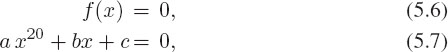
You may think of this equation as a statement of mathematical fact: that the right-hand and left-hand sides of the equation have the same value. You may also view this equation as a challenge: for given values of the parameters a, b, and c, find some values of x that make both sides equal. Although equations usually have variables on both sides of the equal sign, nevertheless, it is also legitimate to write them in generic form:
![]()
where the second version is for our problem. If f(x) is a symbolic expression, then Maple will automatically search for a symbolic solution of f(x) = 0. If f(x) is numeric (contains floats or decimal points), then Maple will conduct a numerical search. We are not using the words “search” and “challenge” just to make mathematics seem exciting. For an arbitrary f(x), there is no guarantee that a solution exists or that Maple will find it even if one does exist.
In many cases, the function f(x) has a form for which no analytic solution exists. To prove the point, even the simple equation
does not have analytic solutions. However, there may be numeric ones, which leads to the somewhat philosophical question “If it is possible to find a numerical solution, does that mean we should also be able to find an analytic solution if we were smarter?” In some cases the answer is “no,” in other cases “yes,” and in others “maybe.” In any case, it is usually faster for Maple to find a numerical solution than an analytic one. Therefore, if your ultimate interest is in a numerical solution, for example to plot a graph, then it makes good sense to have Maple solve the equation numerically in the first place. If you truly want an analytic solution, you may have to rearrange or simplify the equation so that Maple has a better chance with it, or even try some other program, like Mathematica, that employs different algorithms.
5.4 SOLVING A SINGLE EQUATION: SOLVE, FSOLVE
Maple solves equations with the solve command. Let us try it for the general quadratic equation:
We see that there are two roots, and if you look among what might appear to be a garble of symbols, you will see that Maple separates them by a comma (we added some space to make it clearer). Take note that the first argument to solve is the equation to be solved, and the second argument is the variable whose value we want as the solution. We suspect that you think it obvious that since ax2+bx+c = 0 is a quadratic equation in x, that Maple should know that you want the x values that solve it. Yet from an algebraic point of view, the parameters a, b, and c are also symbols for variables, and you may be interested in the solution of this equation for one of them. So try it and observe the differences:
> # Solve the equation for a, b, and then c
As mentioned before, the conventional way to present an equation to be solved is f(x) = 0. Yet once one knows the convention, it is no longer necessary to include the =0 part of the equation. For this reason the same solve command may be used with just f(x):
![]()
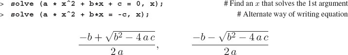
Sometimes the roots of an expression may be a real number, sometimes a complex number containing the symbol I, sometimes an algebraic expression, and sometimes they cannot be found. As long as the solution is exact, the solve command is applicable:
![]()
Yet sometimes even a simple function does not have exact roots:

Confusion seems appropriate after looking at Maple’s response of RootOf(). This is not an answer, but rather an admission of defeat from the internal algorithm used by solve. In this case, the transcendental equation xsinx - 1 = 0 does not have an analytic solution, and so it is no surprise that Maple fails. However, because Maple does not know that the analytic solution truly does not exist, but only that it was unable to find it, Maple blames itself and gives you an indication of where it failed. Knowledge of how and where Maple fails may be useful for advanced work, but for beginners it is easier to rearrange the equation and try again. (Soon we will see that the command fsolve solves this equation numerically.)
Various formulas give closed-form expressions for the roots of quadratic, cubic, and quartic polynomials. And of course Maple knows them. Maple has tricks for higher-order polynomials, and it will try to use them as much as possible. However, there are some higher-order polynomials whose roots Maple cannot find. We give here a case that works, and invite you to change some powers or add some terms until Maple fails (at least for some of the roots):
5.4.1 Verifying Solutions: eval
It is often convenient to use a variable to represent the equation to be solved and thereby avoid rewriting it many times and having very long commands. Suppose the equation to solve contains the product of factors (which makes it easy for us and Maple to know what the solution should be):
![]()
We use a symbol like eqn to represent the entire equation and then work with it:

Once we have a solution, we verify it by substituting it back into the equation with the eval command:
![]()
5.4.2 Symbolic Solution: roots
The solve command is useful for solving equations. Yet sometimes you may have more specialized needs. As an example, you may want to find all the zeros or roots of a polynomial, as well as their multiplicity. The command roots is a powerful tool for finding the exact roots of a polynomial (but not the zeros of a transcendental equation). However, it is specialized to mathematical purposes, and we have often found its use less robust and less obvious than solve. However, it nicely tells us the multiplicity of the root:
![]()
Here the notation [-1,1] in the output means that -1 is a root with multiplicity 1. However, roots is rather limited in that it only works if it is possible to write the roots as algebraic expressions with real integers:
![]()
In this last case the roots are obviously imaginary, so roots just quits. However, adding I as a second argument to roots extends the capability of the algorithm to complex numbers:

5.4.3 Numerical Solution: fsolve
If solve fails to find a solution, or if all you want is a numerical solution, then fsolve, which finds solutions numerically, is the tool to use. As a case in point, we have already seen that solve cannot solve x sinx = 1, yet Figure 5.2 should convince you that there are an infinite number of x values at which x sinx = 1. The problem is that these values are not exact numbers. This calls for the command fsolve, which works just like solve, except it uses floating-point numbers and finds numerical solutions:
![]()
Of course, the above solution is only one solution out of an infinite number, but that is because fsolve finds only one solution at a time. To find more solutions (one at a time), restrict the range of x by modifying the second argument to provide a range:

Figure 5.2 A plot showing that x sin x passes through zero endlessly.

5.5 SOLVING SIMULTANEOUS EQUATIONS (SETS)
5.5.1 Algebraic Equations
If you have a few simultaneous equations to solve, then solve works just fine. If you have a large number, say five or more, then it is probably more convenient and elegant to set your problem in matrix form and use the techniques of linear algebra. We start with two simultaneous equations in two unknowns x and y:
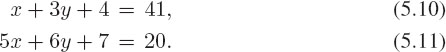
First we assign obvious variable names to the equations:
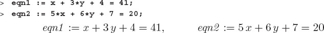
Then we group this set of equations together within braces as to {eqn1, eqn2} form the first argument to solve. Recall, a set is an unordered sequence of distinct expressions enclosed in braces. As the second argument, we enter the set of variables we want to solve for:

Observe how Maple uses braces for its answer set. Verify that the same solution is obtained regardless of the order of the equations {eqn1, eqn2} in their set, or of the variables {x,y} in their set:
> # Enter interchanged equations and variables
This example was fairly obvious, in part, because we used a standard notation for the unknowns and had numerical values for the parameters. Yet consider now the two simultaneous equations:
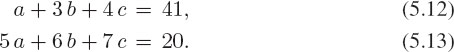
There are clearly two equations and three unknowns a, b, and c. The rules of mathematics being as they are, this means it is possible to solve for any two of the unknowns in terms of the other one, but one unknown will always remain. As before, we first define variable names as labels for the equations:
![]()
We solve simultaneously for {a, b} in terms of the c:

Modify this solution so that it solves for {b,c} in terms of a.
5.5.2 Numeric Equations
For a change of pace, let us say you want a numerical solution of the same two simultaneous equations we previously solved exactly,

The numerical solution should be faster and more reliable than the exact solution, yet Maple knows that it knows the exact solution, and so returns that from fsolve. However we will get the numerical solution if we use decimal numbers in the equations:
![]()
5.5.3 Nonlinear Equations
Nonlinear equations are exactly what their name implies. They are equations containing functions that are not linear. Whereas quadratic, cubic, and quartic equations are all nonlinear by this definition, Maple knows the closed-form solutions to these types of equations and has no trouble applying them. However, there may not be analytic solutions to other, even simple, nonlinear equations. In those cases the best that Maple does is to find numerical solutions.
Consider the simultaneous, nonlinear equations:
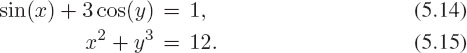
Enter these equations as a set and try solving them with solve. You should not find much success. So, try solving them with fsolve. Use eval to check how well the solution satisfies the equations:
![]()
5.6 SOLUTION TO TOWER PROBLEM
q: Determine an algebraic expression for the height of a five-block tower. ♠
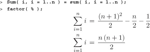
q: Prove that the sum of the first n integers is n(n + 1)/2. ♠ ♠
q: Explain why the height of the tower consisting of n levels is:
![]()
The total height of n noncompressed blocks is nt. However, with our model, each block other than the top one gets compressed. Consequently, the total height is computed by adding the heights of n successively thinner blocks:

However, we recognize the series here as the one we have previously summed and so substitute:

q: Check that this is the same answer as before for a five-story tower. ♠
This agrees with the explicit five-term calculation, namely, H = 5t - 10a.
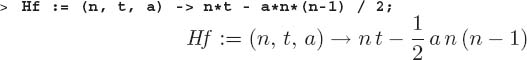
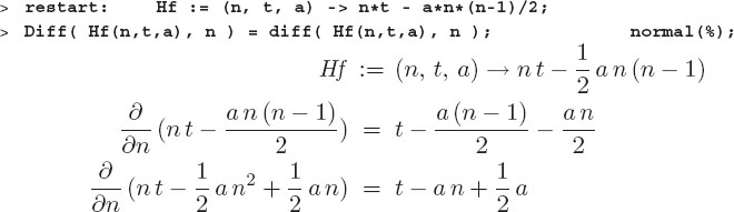
q: Express H as a function of three variables, Hf(n,t, a). ♠
q: Use your function and Maple’s solve command to determine how many blocks n are needed to make a tower of height 200 for arbitrary t and a. ♠
We see that there are two solutions for arbitrary t and a, as expected for a quadratic equation. We suspect that only one of them will be physically meaningful.
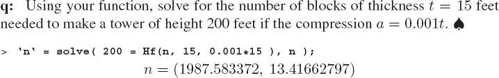
q: Using your function, solve for the number of blocks of thickness t = 15 feet needed to make a tower of height 200 feet if the compression a = 0.001t. ♠
![]()
We get two answers, n = 1987.6 and n = 13.4, neither of them an integer. Because 13 × 15 = 195 and 14 × 15 = 210, the answer 13.4 is the one we would expect. The 1,988-block tower seems unreasonable and is related to a flaw in our model (as we shall see).
q: Is it possible within our model to add another level to the tower but not have its height increase? Explain how the answer to this question is equivalent to finding a solution to the equation H(Nmax) = H(Nmax + 1). ♠
This definition of “maximum” corresponds to adding another block to the tower and not having it get any higher. In some sense this is the maximum height, as adding another block beyond this will actually make the tower shorter in our model. What is happening is that at n=Nmax, the bottom block is being squeezed to zero thickness, and so adding another block gives the bottom block negative thickness. This is clearly a breakdown of our simple model.
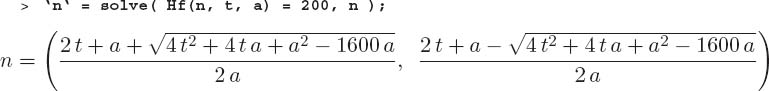
q: Find the algebraic value of Nmax that satisfies this last equation. ♠
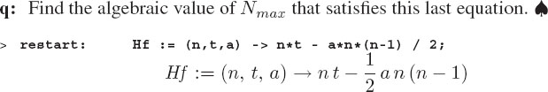
Here we placed both commands on one line and used a colon after restart to suppress Maple’s response. Now we solve it:

q: If t = 15 feet and a = 0.001t, what is the maximum height of the tower? ♠

We could also do the evaluation more explicitly with eval:
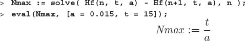
q: Test your function both numerically and symbolically by verifying that adding another level to the maximum number of levels does not increase the height. ♠
where we used the factor command for simplification. ♠
5.7 DIFFERENTIATION: LIMIT, DIFF, D
Calculus was invented, at least from our point of view, to help solve physics problems. Even today calculus is essential for solving scientific problems, and Maple is good at calculus. When speaking of calculus we usually think of differentiation, integration, and differential equations. We study differentiation in this chapter, integration in Chapter 6, and differential equations in Chapter 15.
Derivatives arose in the study of kinematics, where there was the need to define the velocity of an object at each instant of time. Specifically, instantaneous velocity is defined as the limit of the rate of change of position, for infinitesimally small time intervals:

Of course you should recognize this limit as the definition of derivative. Indeed, if we use the active form of Maple’s limit command, we do get the derivative:

Here D(x) indicates the derivative of x, and (t) a function of time t.
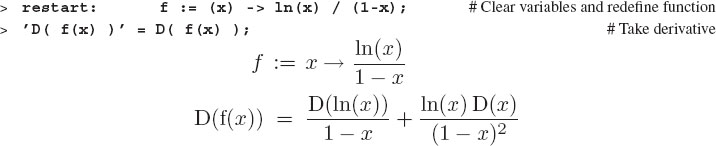
Maple has the two commands diff and D for differentiation. The most straightforward is diff, although D is more powerful and useful. You give diff an expression or a function, and it returns the derivative as an expression. However, if you want your derivative to be a function or a mapping, then use D. (Alternatively, you may use unapply to convert diff’s expression into a function.)
5.7.1 Derivative as Expressions: diff
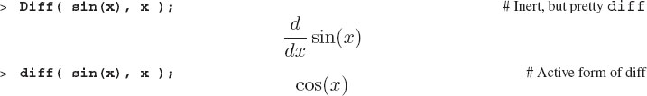
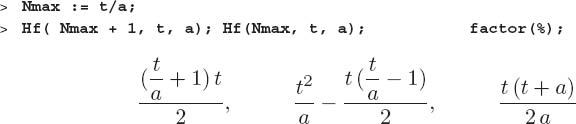
Just as we have seen with sum and Sum, capitalizing the first letter of diff produces the inert form Diff. In spite of inert forms doing no work, they are valuable as a check that Maple will do the computation you intend:
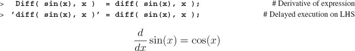
Here we took the derivative of a built-in function sin(x). It is also legitimate to use diff to take the derivative of a user-defined function:
![]()

5.7.2 Second Derivatives
To take a second derivative, you differentiate twice in succession, either by repeating the diff command or by repeating the x part:

In these commands we started with the function f(x) = sin x and took the derivative once with respect to x to get df /dx, and then took the derivative of the derivative d(df / dx )/dx. Executing the above on f(x), as you see, returns us to - sin(x). Taking a derivative of some function twice gives you the second derivative d2f/dx2.
Another notation for second derivative is to use Maple’s sequence operator $. This operator says to repeat the preceding symbol by the number of times indicated after it. To name an instance, x$2 is the same as, x,x. Thus we express higher derivatives in the succinct forms:
![]()

Exercise: Take the first derivative twice of ![]() and see if you get the same answer as taking the second derivative just once ♠
and see if you get the same answer as taking the second derivative just once ♠
5.7.3 Partial Derivatives with diff*
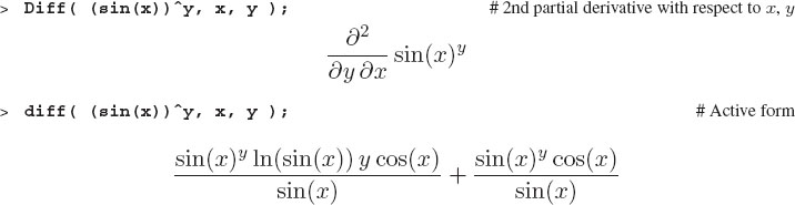
If it is legal only only to take a derivative with respect to a variable, then why must we always enter that variable into diff? The answer is not trivial. On occasion the expression to differentiate may be one like f(x) = sin(x)b. To Maple, both x and b are equally good variables for differentiation, and so Maple must be told which one you would like to differentiate with respect to. At the prompts below, take the derivatives and see the differences:
![]()
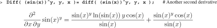
When a function contains more than one variable, then the differentiation process is called partial differentiation. The resulting derivatives are called partial derivatives and in mathematics are denoted with curly d’s, for example, ∂f(x, y)/∂y. In addition, since there are several variables, another type of second derivative is formed by differentiating once with respect to each of two different variables. By way of example, we form ![]() by first differentiating with respect to x, and then y:
by first differentiating with respect to x, and then y:
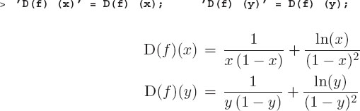
5.7.4 Derivatives of Functions: D
There will be times when you need to have the derivative you calculate be a function or mapping. For cases such as these, the D operator is used to take the derivative of a function (not an expression) and to return the result as another function. This type of derivative and functional analysis is more subtle than the derivatives we have been taking with diff, yet sometimes it is needed to get Maple to do what you want. For instance, consider the two expressions for derivatives:
![]()
The left expression implies the derivative of cos t with respect to t, while the right expression indicates a new function, the derivative of cos, that gets evaluated at t. It is the right type of expression that we want to use as a function. You may think that this is just semantics, yet observe that
![]()
Hence, if the t in d cos t/dt indicates some value, then this is the derivative of a constant, which is clearly 0. Consequently, we must be careful with arguments when we transform one function, such as cos, into another function, such as d cos/dt. The D form of derivative is designed to be used with this type of care. We will look at some examples to see what this means.
Imagine that we are given the position of a mass attached to a nonlinear spring as
![]()
We want to find the velocity v(t) = dx/dt and the acceleration a(t) = dv/dt as functions of time. We first try:
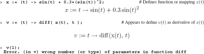
The above response shows that diff(x(t),t) does not work as a proper function when a number is given as the argument. The reason is that Maple does not accept v(1) as the velocity at t=1 although that clearly is what we want. This problem arises from the fact that diff does not produce a true function as an answer. One solution, which we find rather awkward, is to use unapply to convert the expression into a function:
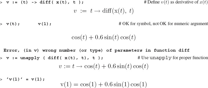
In contrast, the command D produces a proper function that is equal to the derivative of the original function. Scrutinize how the arguments of the functions are implicit and do not have to be (and should not be) specified:
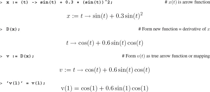
When the derivative function is used as a regular function, for plotting and so forth, its argument needs to be specified. To cite an instance, here we plot position, velocity, and acceleration:
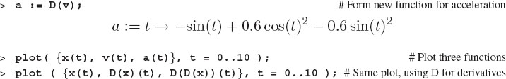
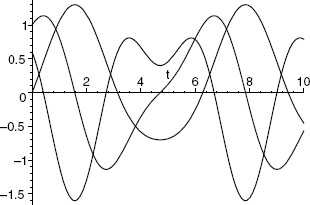
We look now at some more examples of the use of D for creating derivatives of an arrow function:
![]()
OK, we get back what we entered, which may be correct, but is not exciting. This is related to the fact that Maple does not know anything about g. If we give D a function in which the argument is implicit (not given explicitly), then Maple returns the derivative as an implicit function:
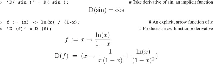
We see that if f(x) is an explicit function of x, then Maple uses the arrow sign to make it clear to us that we have defined a new function of x.
It is best to think of D(f) as an entirely new function, the derivative, and not as an operator acting on f(x). This point is often confusing in the mathematical notation for mappings and transformations (Landau’s second rule). To evaluate this new function obtained by differentiation, we add the argument to D(f), or in this case D(sin):
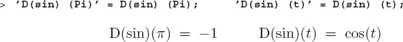
This makes sense if we think that sin is the argument to the D function and that it creates a new function D(sin). This new function, in turn, is evaluated at an argument x. Naturally, we are allowed to take the function D(f) and evaluate it with any argument we want:
Look at how we do not indicate the fact that f is a function of some variable by giving an argument to f within the derivative operation, for example, as D(f(x)). Nor do we state with respect to which variable we are taking the derivative.
In that we are not indicating that the derivative is with respect to x, Maple does not view x as a simple argument, but rather as a general variable or function that has yet to be defined. That being the case, if you ask D to differentiate f(x), it assumes x is some arbitrary function that may have a derivative of its own:
Likewise, since f(15) is just a number, D(f(15)) is the derivative of a constant, which of course is zero:
![]()
As we have said, if you want to evaluate the derivative function for argument 15, then you should think of D(f) as the function:

5.7.5 Second and Partial Derivatives: D
Second derivatives with the D operator are formed either by applying D twice, or by using the composition operator @ (which repeats the action of a function, much like $ repeats the argument):
![]()
With functions of several variables (multivariate functions) such as g(x, y) = sin x cos y, we form different second derivatives by taking the partial derivative with respect to either x or y. You indicate the desired operation to Maple by including a list [in square brackets] of the variable(s) by number that you desire to differentiate with respect to:
Check how Maple indicates these second derivatives as arrow functions (mappings). If the function does not have an explicit definition, then the D operator yields an abstract form:
![]()
Unless the function is very unusual, partial derivatives are generally independent of order:

Clearly then, this option gives us another way to determine the second derivative, even for univariate functions:
5.8 NUMERICAL DERIVATIVES*
Normally you should be happy to have Maple calculate derivatives for you, especially if they are done exactly. If it cannot do it exactly, then let Maple calculate the derivative numerically. We now ask the question, “How does one calculate a derivative numerically?” This query is interesting, as it is useful to understand how Maple does things under cover, as well as being something we will need in Chapter 15, where we undertake a numerical study of projectile motion with friction. Determining a numerical derivative is essentially determining the slope of a function, namely, drawing a tangent to a curve. This is not hard.
Say we want a numerical approximation to the derivative of f(x) = sinx. We know the exact answer,
![]()
The exact derivative is defined as the limit:
![]()
Numerical approximations use a similar approach, except that one skips the limiting process and simply does the division for a small but finite value of Δ:
![]()
So let us try this out on some typical values. We will start with x = 1.0 and Δ= 0.1 (decimal points to ensure that Maple does numerical computations) and compare the approximation to the exact answer:

We see that the approximation is at least close. We make the approximation better by using smaller and smaller values for Δ:
![]()
![]()
The numerical derivative rule we have just outlined is called the forward-difference approximation because it moves forward by Δ to sample how the function changes. A more balanced rule that requires no extra computation is known as the central difference approximation. It evaluates the function on either side of x and takes that difference:

We apply it with the same values of Δ as used for the forward difference:
We see that even the largest value of Δ yields three places of precision, with the approximation still improving as Δ is made smaller still. Notwithstanding the use of even more precise algorithms in scientific work, our exercise here should convince you that numerical derivatives are generally reliable.
5.9 ALTERNATE SOLUTION: MAXIMUM TOWER HEIGHT
If we think of Nmax as a continuous variable and take a mathematical point of view, then the maximum height occurs at the point at which an infinitesimal change in n leads to no change at all in the tower’s height. We know from calculus that this occurs when the derivative vanishes, that is, when dH(n, t, a)/dn = 0:
q: Use Maple’s derivative function diff to determine dH(n, t, a)/dn. ♠
q: Before we defined the “maximum” tower height as one for which H(Nmax + 1) = H(Nmax), now we want to use calculus. Use Maple’s solve function to determine the value of n for which dH/dn = 0. ♠

q: Explain in your own words why this is not the same as Nmax. ♠
Our previous definition of Nmax was one for which Nmax and Nmax+1 both gave the same height. That definition gave Nmax = t/a and Nmax + 1 = (t + a)/a as producing the same height. The derivative vanishes at (t + a/2)/a, which is right between our previous two answers. Neither one is really more correct, but they do correspond to different definitions of maximum.
q: Plot up the results as a check. ♠
It is not possible to make plots of symbolic functions, so let us assign values to t and a. We know from our computations that the maximum, in some sense of the word, occurs near n = 1000, so we will narrow our plot to that region:

We do indeed see that the maximum height, as determined by the zero of the derivative, occurs at the true maximum of the graph, n = 1000.5, but that in terms of integer block numbers, there are maxima at n = 1000 and 1001.
5.10 ASSESSMENT AND EXPLORATION
1. How relevant is this model to building actual skyscrapers? Specifically, is it wise to use the same structural design on the top and bottom floors?
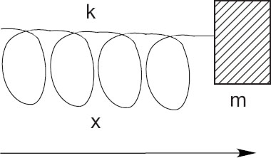
Figure 5.3 A mass m attached to a spring with constant k that is stretched a distance x from its equilibrium position.
2. It is not realistic to have the addition of levels make the tower shorter. Explain in words whether an assumption is at fault, or are we just applying the model beyond its range of applicability.
3. Rather than (5.1), a more realistic model might assume that the blocks get harder to compress at some point and so their thickness never becomes negative. An equation that describes this model may be
![]()
where t is the thickness of a single block supporting i blocks above it, and b ~ 1/100 is a small number. Obtain an expression from Maple for the total height of a tower of N blocks. Hint: while the sum is simple, Maple may not be able to come up with a simple answer. However, numerical evaluation is possible.
4. Use the improved model to derive a Maple function that calculates the height of a tower containing N blocks.
5. Is there a maximum height for the tower now? Plot up the results to be sure.
6. The rate of increase of the tower height with number of blocks is given by the derivative dH/dn. Is there some value of n for which the rate of increase is a maximum? What is the numerical value for the maximum height now (use similar parameter values as before)?
5.11 AUXILIARY PROBLEM: NONLINEAR OSCILLATIONS
A mass m = 2kg is attached to a spring as in Figure 5.3. The mass is displaced from its rest position and then released so that it oscillates about the equilibrium position. When the mass is a small distance x from the equilibrium position, the restoring force f tending to bring the mass back to equilibrium is directly proportional to x:
![]()
where k is the spring’s force constant k = 25 Newton/meter. The equation of motion for this system is Newton’s second law of motion:

As shown in the study of simple harmonic motion, a solution for the position x as a function of time t is a trigonometric function,
![]()
1. Write a Maple function that returns the position x(t) for any input argument t. (You are given numerical values for m and k, and therefore for ω.)
2. Plot the position for times in the range 0 ≤ t ≤ 12. As always, add labels and a title to your plot.
3. In mechanics we learn that the velocity v is the first derivative of x with respect to time, and that acceleration a(t) is the second derivative:

Use Maple’s diff command to determine analytic expressions for velocity and acceleration as functions of time.
4. Determine whether (5.19) is true for this oscillator, that is, compare ma to the force -k x.
5. Plot x(t), v(t), and a(t) in the same graph for t between 0 and 10, with different colors for each of the three functions.
6. Take your plot and change some lines to dotted and some to bold. Which scheme do you think is clearest?
7. Make a phase-space (parametric) plot of v(t) versus x(t) to produce v(x).
8. A more realistic model for an oscillator has the restoring force acting upon the mass depend slightly upon whether the mass is to the right or to the left of the origin (nonlinear terms). For this case the position as a function of time might be described by
![]()
where b (which controls the right-left asymmetry) is a small number compared to 1. 9. Modify your Maple function x(t) to a new one x(b, t) and test that you get the old answer for b = 0.
10. For this new oscillator, what are the velocity, acceleration, and force as functions of time? Make several plots for a range of b values between 0 and 1. Add comments to your worksheet indicating for what b values the functions no longer look sinusoidal.
11. Use a 3-D plot with axis and labels to examine x as a function of time for the entire range of b values. Examine the different options for displaying your surface, as well as different viewing angles. Print out several of the best representations (assume that the printer prints grayscale only). Make sure one of your plots is of only the actual points that are calculated (no connecting lines) and that another one is of contours.
12. Examine the v(t) versus x(t) phase-space plot for this anharmonic oscillator for a number of b values.
13. Make a parametric plot of the force f(t) = ma(t) versus position x(t) for this anharmonic oscillator. Determining an analytic expression for f(x) would be more difficult.
14. Create two animations of this function, one in which the different frames correspond to different b values, and a second in which the different frames correspond to different times. Look at both and decide which produces the best visualization (animations are usually best to show time dependence).
5.12 KEY WORDS AND CONCEPTS
analytic solution |
derivative |
derivative operator |
limit |
mapping |
maximum |
numerical solution |
partial derivative |
roots |
simultaneous equations |
theory vs. model |
1. Give three possible meanings of the words maximum height.
2. Are mathematical equations always true?
3. Must all equations have analytic solutions?
4. If an equation has a numeric solution, must it also have an analytic solution?
5. Do nonlinear equations occur in nature?
6. How are simultaneous equations different from other types?
7. Are all solutions to an equation equally valid?
8. Are nonlinear equations harder to solve than linear ones? If so, why?
9. Do you have to take a limit to evaluate a derivative?
10. Does it make sense to take the derivative of a function of several variables?
11. What is the difference in Maple between taking the derivative of an expression and a function?
12. Can you take the derivative of a number?
5.13 SUPPLEMENTARY EXERCISES
1. Use both solve and fsolve to find as many solutions as you are able of
a. x3 + x2 + x = 1.
Beware, this equation may have complex roots that fsolve will not show unless you include complex in the argument set: (fsolve(f(x),x,complex).
b. x4 + cx3 + x2 + x + 1. Hint: you may need to make c numeric.
c. sin(x)2 = x. Make a plot to check that your answer is reasonable.
2. Determine the limit
a. ![]()
b. ![]()
c. ![]()
d. ![]()
3. Determine the first and second derivatives with respect to x of the following expressions:

4. Nonlinear equations are more interesting, but more challenging to solve, than linear equations. They are called nonlinear because the unknown appears to a higher power than the linear first power. Find the solutions of the nonlinear, simultaneous equations:
![]()
5. You are given the expression 10 x4 sin(k x).
a. Enter this as a Maple expression and determine when it equals 0, and its first and second derivatives.
b. Enter this as a Maple function and determine when it equals 0, and its first and second derivatives.
6. In mechanics, we often study the position x of an object as a function of time t. If we take the first derivative of the position with respect to time, we get the velocity v as a function of time. In turn, the acceleration a is the second derivative of x with respect to time. In the following exercises, calculate x(t), v(t), and a(t) for each case, and plot all the functions on the same graph as a function of time for 0 ≤ t ≤ 10. Use different colors for each function:
7. Here is a real function of the variables x, y, and z:

Check whether g is a solution of Laplace’s differential equation by showing that the sum of these three derivatives equals 0:

8. Find the first and second derivatives with respect to x of the functions:
9. A rock is hurled upward, and its distance above the ground is given by y= 210 t - 34 t2. Use Maple to calculate:
a. the maximum height from the ground of the rock,
b. the time at which the rock reaches the maximum height,
c. the time at which the rock strikes the ground,
d. the rock’s speed when it hits the ground.
10. The resistance R of two resistors in parallel is given by
![]()
Solve for R and take the limit as R2 approaches infinity. Does your answer make sense?