Chapter Seventeen
Arrays: Vectors, Matrices; Rigid-Body Rotations
Vectors and matrices play key roles in scientific computing. Indeed, much of so-called high-performance computing involves computations with very large arrays. These arrays may contain experimental data needing processing, or they may contain the results of a simulation in which the discrete nature of breaking space up into small units leads naturally to the use of arrays. And since real-world problems are often complicated and require high precision (small units), arrays with thousands or millions of elements are not unusual. Even though this means that the matrices used in realistic problems will be big and will require efficient algorithms, often the programs using matrices are simple and direct.
In this chapter we deal with techniques needed to create and manipulate vectors and matrices in Java. We will solve the same problem as we did with Maple in Chapter 7, “Matrices and Vectors; Rigid-Body Rotation.” If needed, you should review that chapter for some of the physics and mathematics background (even elementary stuff like what a vector is), and then return here for the Java approach. In an optional section of this chapter we discuss Jama, a library of linear algebra methods in Java, that deals with true matrix objects.
It is interesting to observe how the Java and Maple approaches to this problem tend to complement each other. Maple is able to do the calculations symbolically, whereas Java is not. However, Maple is slow in performing numeric calculations involving large matrices, while compiled languages tend to be much faster. In addition, Maple excels in its capacity for interactive 3-D graphics, while this is harder to do in Java or even Mathematica. There are Java packages available that permit interactive 3-D graphics, but they are too complicated or too expensive for us to treat here.
17.1 PROBLEM: RIGID-BODY ROTATIONS
Your problem is similar to the one in Chapter 7. Here we will deal with a plate and a square whose moments of inertia are given, and we will focus on the matrix multiplication that converts the angular velocity ω into the angular momentum L.

Figure 17.1 Left: A plate sitting in the x – y plane with a coordinate system at its center. Right: A cube sitting in the center of a three-dimensional coordinate system.
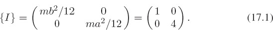
Problem 1: Consider the two-dimensional rectangular metal plate shown on the left of Figure 17.1. It has sides a = 2 and b = 1, mass m = 12, and inertia tensor for axes through the center:
The plate is rotated so that its angular velocity vector ω always remains in the x-y plane (which does not mean the plate remains in the x-y plane). Specifically, it is rotated with the three angular velocities:
![]()
Write a Java program that computes the angular momentum vector L via the matrix multiplication L = {I}ω. Plot ω and L for each case, and compare the results to those found with Maple.
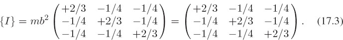
Problem 2: Consider now the rotation of the cube on the right of Figure 17.1. The cube has side b=1, mass m=1, and, for axes on the corner, an inertia tensor [M&T 88]:
The cube is rotated along axes passing through two sides and the diagonal, explicitly, with the three angular velocities:
![]()
Write a Java program that computes the angular momentum vector L via the requisite matrix multiplication. Plot ω and L for each case, and compare the results to those found with Maple.
17.2 THEORY: ANGULAR-MOMENTUM DYNAMICS
Recall from Chapter 7 that the angular-momentum vector L is given by the product
![]()
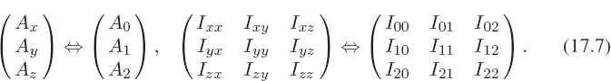
Here ω is the angular-velocity vector and {I} is the inertia tensor represented by the matrix [Iij ]:
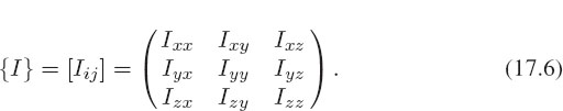
Despite the use of x, y, and z to label the three axes being standard in elementary science, the mathematics and the computing gets easier if we label each direction with a number rather than a letter. Consequently, we now change to a notation in which A0 indicates the component of the vector A in the x or “0” direction, A1 indicates the component in the y or “1” direction, and A2 indicates the component in the z or “2” direction:
Here we use 0, 1, 2 for the indices rather than 1, 2, 3 to be consistent with Java conventions for array elements.
With this new notation, the relation stating that the angular momentum equals the product of the moment of inertia tensor times the angular-velocity vector is represented by the matrix multiplication:

In terms of the individual components, (17.8) is an elegant way of representing the three simultaneous equations:

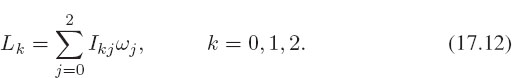
These three equations may also be written in a convenient form for computations:
17.3 CS, MATH: ARRAYS, VECTORS, AND MATRICES
We saw in Chapter 16’s dealing with complex-number objects, how the mathematics and the programming become simpler if we deal with a variable’s single name, even though it has multiple parts. In computer science we store an entire table of numbers in a single variable when that variable is declared as an array. You then deal with the entire array as one symbol, or deal with individual elements in the array via a subscript or index notation. As a case in point, we store the final exam scores of all students in the array Final[i], with the different values of the index i referring to different students. In this case, Final[10]= 99 would be the score of student number 10, and Final[100] = 13 would be the (sorrowful) score of student number 100.
There is no requirement that arrays have only one index. To prove the point, we could use the 2-D array HW[i][j] to store all homework scores for all students, with i representing the assignment number and j representing the student number. It follows then that HW[2][3]=99 would be second homework score for student number 3, while HW[10][500]=12 would be the tenth homework score for student 500.
You may think of a CS array as an abstraction of the mathematical idea of matrices and vectors. Arrays are collections of values of a certain data types, which themselves may be either abstract or intrinsic types. The values contained in an array are called elements, and the shape of an array is referred to its dimensions.
Actually, 2-D arrays are stored in Java as a 1-D array, with each element of the 1-D array being another 1-D array representing a row of elements:
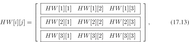
where each box is an independent 1-D array. This means, as we shall see, that we may then assign values to each row in a single command, and that we may even make each row independent objects from the other rows.
In mathematics and science we deal with objects called vectors and matrices. Taking into account that only one index is needed to distinguish the components of a vector, they are stored on a computer in a 1-D array. Because matrices have rows and columns, their elements are stored in arrays with two indices. As an example, the matrix Ixy, representing the inertia tensor, could have its components stored in the array I[x][y]. To repeat, the mathematical objects are vectors and matrices, the computer storage is in single-indexed and double-indexed arrays. (In a later section of this chapter we discuss Jama, an extension of Java that deals with objects that are true matrices.)
As is often the case when science and computer science are combined, confusion results from using different words to describe the same idea. Even worse, we often use the same words to describe different ideas. Of necessity we now must point out that our use of the words “two-dimensional” and “three-dimensional” is from physics, where the number of dimensions of space equals the number of components (indices) that a vector may have, and where the number of values that any one index spans is also equal to the number of dimensions. Yet on a computer, a “three-dimensional array” refers to a data type with three indices, such as A[i][j][k], and there is no limit on the range spanned by any one of the indices i, j, and k. In the latter case, the maximum value of some index is referred to as the “size” or “length” of the array, not its “dimension.” To name an example, the two-dimensional physics vectors used to describe motion in a plane are stored in one-dimensional arrays of length 2.
Recall how in Chapter 16, “Object-Oriented Programming,” we used a single object, or abstract data type, to store the real and imaginary parts of a complex number. Java represents arrays as objects, with the size of the object determined by the programmer, and with the individual components of the object referenced by array indices. Explicitly, the elements of an array are referenced by giving each index in a square bracket after the array name, for example, R[1] or I[x][y].
As we saw for complex objects, arrays also must be declared and created. Declaration tells the compiler the name of the array and the type of data elements to be stored in it. Creation reserves a place in memory for the array elements. The syntax for array declaration is similar to that used for primitive data-type declaration, but now with empty square brackets following or preceding the array name:
![]()
After declaring an array to exist, we must also create the place in memory for it by using the new operator (as we also did for complex objects):
![]()
As with complex objects, declaration and creation may be combined in one line:
![]()
An important variation on this one-line declaration is the ability to declare, create, and initialize Java arrays in one step with the initializer convention. By entering a list of comma-separated values enclosed in curly braces, we accomplish these three tasks in one fell swoop:
![]()
where this initializer may be used only in a declaration statement. Observe how the declaration does not specify the size of the array in these examples. That is done by the creation step that includes a number within the square brackets, or by explicit initialization. For the array R this is length 3, which means that it contains the elements R[0], R[1], and R[2].
A common error in dealing with arrays is going out of bounds, that is, telling the computer to go to a location in memory that does not contain any of your array’s elements. This error is easy to make. Even though we declare double R[length], the last element of the array is R[length-1] since the index count starts at 0 and not 1. Java is all too happy to tell you (again and again) that you have made this mistake, and then not compile your program for you; other languages may let you go beyond the declared size, which is not good because you may end up someplace where you do not belong.
Listing 17.1 OneDArray.java

Example and exercise: The program OneDarray.java in Listing 17.1 sets up two vectors A and B, each of length 10,000, and then forms the cross product A×B.
1. Compile and execute this program. Examine the way the last line gives you the time it took Java to run your program (execution time). This was obtained by calling the Java utility program, System.currentTimeMillis() that reads the clock on the wall in milliseconds.
2. Place the three 1-D vectors A, B, and C into a single 2-D array. You may do this with statements of the form:
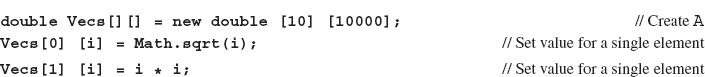
3. Compile and execute the 2-D version of the program and note how much longer it now takes to run. The extra time arises from the computer having to move through larger blocks of memory.
4. Modify OneDarray.java to print out values for A[0], A[999], and A[1000] .
Java should not let you access an element that is out of bounds. ♠
17.4 IMPLEMENTATION: INERTIA.JAVA, INERTIA3D.JAVA
For our rotation problem, implemented in Inertia.java and Inertia3D.java,
we will represent the vectors L and ω with the 1-D arrays L and w, and the inertia tensor {/} with the 2-D array I. We have showed you how to declare these arrays in Java and how to reserve memory locations for them, but we have not actually placed any values for them in memory. The most direct way to assign values to an array is by assigning values to each individual element. By way of example, if our angular velocity vector ω were pointing along the × axis with magnitude 10, then we would assign it the three components:
![]()
Declaring values for the moment of inertia tensor I is more interesting since it is a 3×3 array. Again, we explicitly list each individual element, for example,

In addition to creating multidimensional arrays by using the new statement, we may also create them by explicitly listing values for all the elements using the initializer convention. When entering values for an entire array, an entire row of values is entered as if it were a single element corresponding to the second index. Wherefrom you may think of a 2-D array in Java as a 1-D array of rows:
![]()
Indeed, although we will not have any need for it in this chapter, it is also possible to build up an array with each row having a different length, or with the elements of an array being sub-arrays. In this way, arrays are used to build some structured data sets. To repeat, a 2-D array is entered as a 1-D array of 1-D arrays.
The number of elements contained within an array is referred to as its length. In Java, an array is an object with length as one of its properties, and we extract that property with a dot operation; for example, A.length is the length of array A:

In ArrayLength.java on the CD, we demonstrate how to determine the length of a 2-D or 3-D array. Recall that a 2-D array is constructed as a 1-D array of rows, with each row stored as independent 1-D arrays. Because each row may have different lengths, we need to specify that row in which we are interested:

17.4.1 Arrays as Arguments to Methods
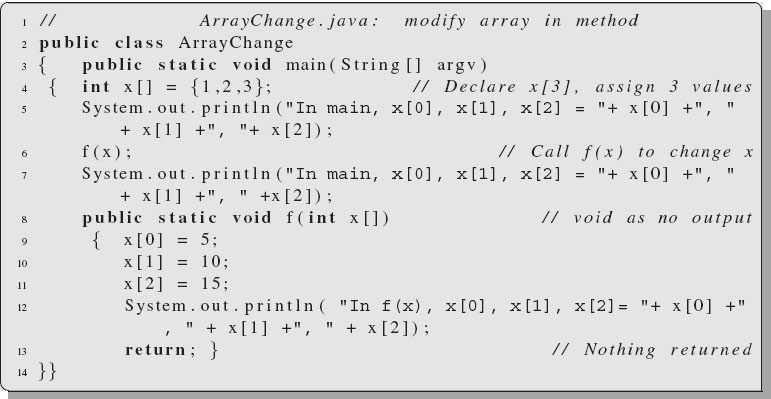
Now we break two of the rules we stated in Chapter 10, “Data Types, Limits, Methods.” We told you there that a method returns only one number as its value, and that changes made to arguments are not returned to the calling program. The exceptions to these rules occur when an array (or any object) is used as the argument to a method. Inasmuch as an array is an object with multiple parts, when a method is called with an array as an argument, Java passes the location in memory where the object is stored instead of the values of its individual parts. For instance, if we pass the array x[3] as the argument to a method f(x), then method f cannot change the value of the address in memory where storage of the three elements of x begins, but it is free to change the actual values x[0], x[1], and x[2] that are stored there. And since the calling program goes to the same locations in memory, it will find the changed values there. Since the argument to the method is an address that does not get changed, Java does not flag this scheme as an error. For example, the code ArraysEqual.java on the CD shows that if two arrays are set equal to each other, then they share the same locations in memory, and so changing the values of one automatically changes the values of the other.
To see how this works, run the code ArrayChange.java in Listing 17.2. Check that all three values of x are changed by the method f(x), but none are returned to main as arguments. Nevertheless, the changed values of x are seen by main method. In fact, f returns nothing to main, as indicated in f’s declaration statement by void as its data type. The return statement is needed, but only to get back to main.
Listing 17.2 ArrayChange.java
17.5 JAMA: JAVA MATRIX LIBRARY*
Jama is a basic linear algebra package for Java, developed at the US National Institute of Science [Jama]. We recommend it since it works well, is natural and understandable to non-experts, is free, and helps make scientific codes more universal and portable. Other scientific subroutine libraries in Fortran and C, such as Lapack [LAP 95], have made valuable contributions to science by providing numerical techniques that are more efficient and reliable than those a scientist or engineer might write in the course of solving a problem. Jama provides object-oriented classes that construct true Matrix objects, add and multiply matrices, solve matrix equations, and print out entire matrices in aligned row-by-row format. Jama is intended to serve as the standard matrix class for Java.1
17.5.1 Jama Examples
The first example deals with 3 × 1 vectors b and x, and a 3 × 3 matrix [A]:
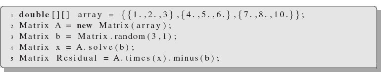
The vectors and matrices are declared and created as Matrix variables, with b given random values. It then solves the 3×3 linear system of equations {A}x = b with the single command Matrix x = A.solve(b);, and computes the residual {A}x - b with the command Residual = A.times(x).minus(b);.
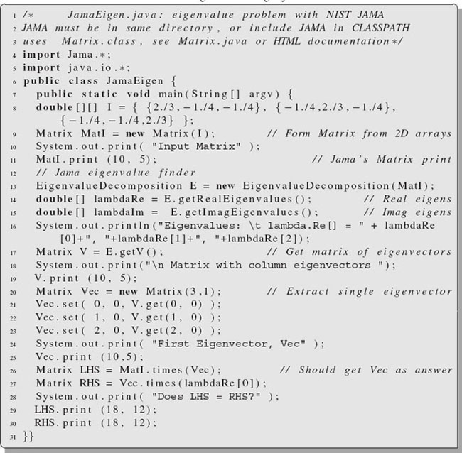
Listing 17.3 JamaEigen.java
Our second Jama example looks at the same problem examined in §7.7, namely, finding the principle-axes system for a cube. We discussed the idea that there is a coordinate system in which this inertia tensor is diagonal, and that finding such a system entails solving the eigenvalue problem,
![]()
where {I} is the original inertia matrix, ω is an eigenvector, and λ is an eigenvalue. The program JamaEigen.java in Listing 17.3 solves for the eigenvalues and vectors, and produces output of the form:

Look at JamaEigen and notice how on line 8 we first set up the array I with all the elements of the inertia tensor, and then on line 10 we create a matrix MatI with the same elements as the array. On line 13 the eigenvalue problem is solved with the creation of an eigenvalue object E via the Jama command:
13 EigenvalueDecomposition E = new EigenvalueDecomposition(MatI);
Then on line 14 we extract (get) a vector lambdaRe of length 3 containing the three (real) eigenvalues, lambdaRe[0], lambdaRe[1], lambdaRe[2]:
14 double[] lambdaRe = E.getRealEigenvalues();
On line 17 we create a 3×3 matrix V containing the eigenvectors in the three columns of the matrix with the Jama command:
17 Matrix V = E.getV();
which takes the eigenvector object E and gets the vectors from it. Then, on lines 21–23, we form a vector Vec (a 3×1 Matrix) containing a single eigenvector by extracting the elements from V with a get method, and assigning them with a set method:
21 Vec.set(0,0,V.get(0,0));
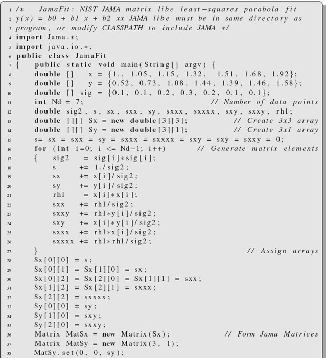
Our final Jama example is the program JamaFit.java in Listing 17.4. It demonstrates many of the features of Jama. It makes a least-squares fit [CP 05] of the parabola y(x) = b0 + b1x + b2x2 to a set of ND measured data points:
![]()
where ±σi is the uncertainty in the ith value of y. The fitting is realized by finding a solution to the three simultaneous linear equations:
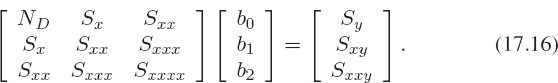
Here the S’s are various sums over the data:

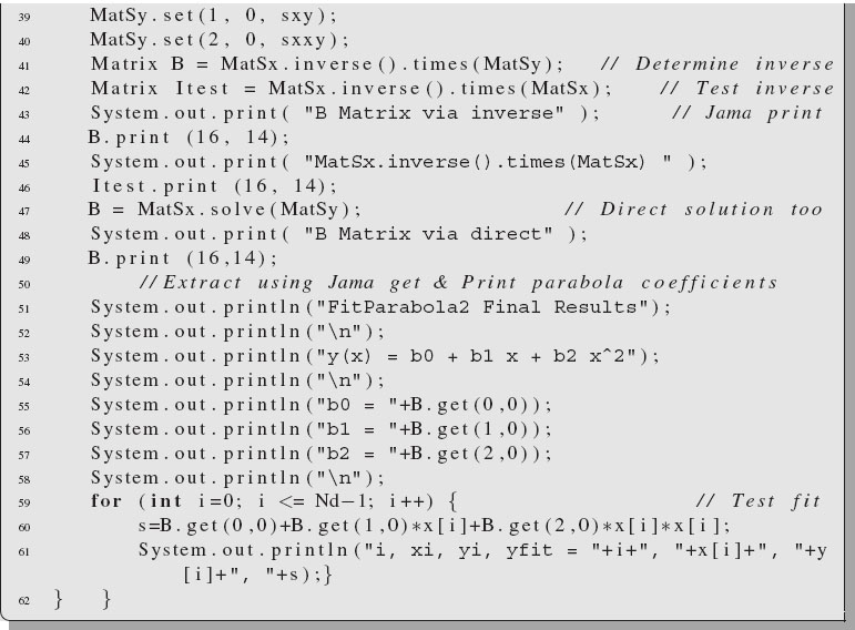
Listing 17.4 JamaFit.java
17.6 KEY WORDS
angular momentum |
angular velocity |
arrays |
arrays as arguments |
declaration |
creation |
dimension |
eigenvalue problem* |
inertia tensor |
initializer |
linear equations* |
matrix library |
matrix multiplication |
rigid bodies |
rotation |
Explain in just a few words what is meant by:
1. a subscript and an array index being different;
2. an abstract data type;
3. a complex number;
4. a Java object;
5. an array;
6. the dimension of an array;
7. the length of an array;
8. a class variable;
9. a local variable;
10. the difference between a class and a method.
17.7 SUPPLEMENTARY EXERCISES
1. Do problems 1 and 2 from the beginning of this chapter!
2. Consider the program arrayChange.java given in Listing 17.2. We declared x to be an array of integers, created the array, and assigned it values all on one line with. Modify the program so that only the declaration and creation are done in one statement. Do the creation using the new command and the assignment in a different statement.
3. We used an integer array as the argument for our method. Modify the program so that x[] is now a double of length 5, rather than 3. Test your method by printing out the 5 doubles before and after the method call.
4. There is no reason that the method f(x[]) cannot also do some calculations and return a value for f(x[]) as well as changing the values of x[]. Modify ArrayChange.java so that the method calculates and main prints out the norm
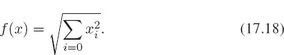
5. What we have said about methods dealing with single-indexed arrays hold equally true for multi-indexed arrays. Modify the program so that x[3] is now the two-indexed array x[3][2], and assign values to x[i][1] for i = 0, 2.
1 A sibling matrix package, Jampack [Jampack] has also been developed at NIST and the University of Maryland, and it works for complex matrices as well.