Chapter Seven
Matrices and Vectors; Rigid-Body Rotation
7.1 PROBLEM: RIGID-BODY ROTATION
The study of rotations in classical mechanics is an excellent example of the use of vectors and matrices in science. The problem we study is basically an exercise that we work out in full and ask you to repeat for another case. For comparison, we repeat this same problem using Java matrices in Chapter 18. Even if you are not familiar with the physics, we suggest that you work with us through these examples as a review of matrices and as a preview of what is to come; it should also make learning the physics easier in the future.
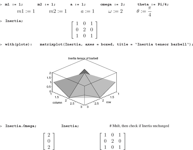
Problem a (we work this one through for you): Consider Figure 7.1 showing a barbell composed of a mass m1 attached to mass m2 by a massless rigid rod of length 2a. The barbell is fixed at an angle θ with respect to the z axis, and is being rotated with an angular velocity vector ω along the z axis.
a. Use Maple to determine the vector angular momentum L of this barbell by adding up the angular momenta of the two masses.
b. Use Maple to evaluate the inertia tensor {I} for this barbell.
c. Form the matrix product {I}ω of the inertia tensor and angular velocity for the barbell. Check that you get the same value for L as above.
d. Make 3-D plots of L and ω for three different times, and thereby show that L rotates about a fixed ω. A changing L implies that there is an external torque being applied to the barbell.

Figure 7.1 A barbell rotating about a fixed axis in the z direction. In Maple you can grab and rotate this pointplot3d figure.

Figure 7.2 Left: A 2-D rectangular plate of side 2 with the origin at its center and a mass at each corner. Right: A cube of side 2 with the origin at its center and a mass at each corner. In Maple you can grab and rotate these pointplot3d figures.
Problem b: Consider the 2-D square plate on the left of Figure 7.2 with a mass m at each corner. It is rotated with these three values for the angular velocity:
![]()
1. Use Maple to determine the angular momentum vector L of the plate by adding up the angular momenta of the individual masses.
2. Use Maple to evaluate the inertia tensor {I} for this plate. Hint: if this were a solid plate, its inertia tensor would be
![]()
3. Form the matrix product {I}ω of the inertia tensor {I} and angular velocity ω for the plate, and check that you get the same value for L as before.
4. Make three 3-D plots of L and ω for different times, and thereby show that L rotates about a fixed ω. From this we deduce that there must be an external torque applied to the plate.
5. Determine the torque acting on the plate. (optional)
Problem c: Consider the 3-D cube on the right of Figure 7.2 with a mass m at each corner. It is rotated with these three values for the angular velocity:
![]()
1. Use Maple to determine the vector angular momentum L of the cube by adding up the angular momenta of the individual masses.
2. Use Maple to evaluate the inertia tensor {I} for this cube. Hint: if this were a solid cube, its inertia tensor would be

3. Form the matrix product of the inertia tensor and angular velocity {I}ω for the cube and check that you get the same value for L as above.
4. Make some 3-D plots of L and ω for different times. Thereby show that L rotates about a fixed ω. From this we deduce that there must be an external torque applied to the cube.
5. Determine the torque acting on the cube. (optional)
7.2 MATH: VECTORS AND MATRICES
Classical mechanics is an area of physics that studies the motion of particles and objects. Before we describe the motion of a particle, we must first develop a system to specify the location of a particle in space. As illustrated in Figure 7.3, we describe the location R of a point in space by drawing a set of perpendicular x and y axes, and then drawing a line from the origin O to the point R. An arrow head is usually added to this line segment to show its direction. An arrow in space is the most elementary representation of a vector.
We view Figure 7.3 as showing a graphical representation of the displacement vector R. This vector has length or magnitude R = |R|, and a direction specified by giving the angle θ that the vector makes with the x axis. A vector is usually denoted by a bold symbol, such as R, or sometimes by a symbol with an arrow over it. By convention, the magnitude of a vector is denoted by the same symbol used to denote the vector, only without the bold font or arrows. Even though the direction and magnitude of a vector is a good way to visualize a vector, calculations on vectors are usually easier to perform with the individual components of the vector. For our vector R, its components are just its projections along the positive x and y axes:
![]()
Thus, if we know R and θ, it is easy to use these equations to calculate x and y, or if we know x and y, R and θ:
![]()
Usually these components are put together inside some kind of parentheses to indicate that they are the components of a single object. Within the text of a document, they may be written in a horizontal row as (x, y), while in an equation they may be grouped as a vertical column:

Figure 7.3 Left: Representation of a vector as an arrow in 2-D space. Right: Representation of a vector as an arrow in 3-D space. The projection of the arrow along each axis equals the components of the vector. In Maple you can rotate the 3-D figure.
![]()
Whether a vector is viewed as an abstract symbol R or as the collection of components, it is the same object being viewed. Multiple representations are a good thing, because sometimes it is easier to perform formal manipulations with abstract symbols rather than individual components, while other times it is easier to perform explicit calculations with the components.
We have drawn the vector R as if it were in a plane. If you spent more time away from the computer screen, you might realize that the real world has three dimensions, and we really should be drawing our vectors in a 3-D space with components along the x, y, and z axes. As shown in Figure 7.3, while the trigonometry is more complicated for 3-D vectors than 2-D ones, working with components is much the same, only now R has three components:

Other vectors in addition to the displacement vector R occur regularly in science. Examples include velocity, acceleration, force, and electric and magnetic fields (so you may as well start to understand them now if you do not already). Fortunately, the rules for decomposition into components are the same for all vectors, as are the rules for various algebraic manipulations.
7.2.1 Vector Operations and Matrices
Operating upon vectors that are represented by components is really quite easy, since all you have to do is operate on the individual components using the ordinary rules of algebra. To illustrate, let us say we have vectors A and B represented by their three components,

Addition and subtraction are defined as

Multiplication of vector A by a constant c is defined as

Two vectors may multiply each other in two ways. The dot product is the sum of the product of their corresponding components:
![]()
where the bar over the components of A indicates complex conjugate. In science, the asterisk * is usually used to indicate complex conjugation, yet is often left off, since the vectors are real. Geometrically, the dot product A•B is just the projection of A along the direction of B. In view of the fact that the result is just a scalar (a quantity with no direction), the dot product is also known as the scalar product.
The second kind of vector multiplication is the cross product:

Geometrically, the cross product A×B is a new vector perpendicular to the plane formed by A and B, with magnitude |A||B|sinθ, where θ is the angle between the vectors A and B.
7.3 THEORY: ANGULAR MOMENTUM DYNAMICS
A rigid body is one in which the distance between the particles that compose the body do not change [M&T 88]. We imagine such an object rotating about a fixed point O (or about the center of mass of the body). In spite of it being true that each part of a rotating body has a different velocity, all parts have the same angular velocity ω. The velocity of part i is related to ω via:
![]()
where ri is a vector from the origin O to part i, and × represents the vector cross product.
Angular momentum is introduced into mechanics as the rotational analog of linear momentum. It measures the tendency of a rotating object to remain rotating, and has a direction associated with it. For the highly symmetric cases usually studied in elementary physics, the angular momentum and angular velocity vectors are parallel to each other,
![]()
with the proportionality constant I called the moment of inertia. However, when an object rotates about an axis that is not one of high symmetry, then L and ω will not be parallel to each other, and a generalization of this equation is needed. The general relation between the angular momentum and the angular velocity follows from expressing the angular momentum of a group of particles as the sum of the angular momentum of each particle:
![]()
where pi =mivi is the linear momentum of particle i. If we restrict ourselves to the rotation of a rigid body about a fixed point, then the velocity is related simply to the angular velocity, and we have
![]()
where the right-most vector cross product must be performed first.
We now skip over the details of the derivation and give you the final result. For general problems, such as rotation of the cube in Figure 7.3 about axes along a side of the cube, the angular velocity ω and angular momentum vector L are related by what Maple calls the dot product of vector ω with the inertia tensor {I}:
![]()
Observe how in the above equation we have placed braces around the symbol I. The braces indicate a type of mathematical object, a tensor, that transforms one vector into another vector. If the vectors are represented by columns (the usual thing), then we represent the action of a tensor on a vector by the multiplication of that vector by a matrix:

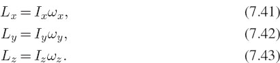
We see by looking at this equation, and by applying the rules of matrix algebra, that this one matrix equation is an elegant way of presenting the three simultaneous linear equations relating the individual angular velocity and angular momentum components to each other:

It is, of course, even easier to write this as one matrix equation L = ω. In addition, it is much easier to manipulate the matrix equation than the individual equations.
The diagonal elements Ixx, Iyy, and Izz of the inertia tensor are called the moments of inertia about the x, y, and z axes, respectively. They are the same as those used in elementary physics. The off-diagonal elements, such as Ixy = Iyx, are negatives of what are called products of inertia, and they are responsible for making ω and L nonparallel. An explicit expression for the elements of I is [M&T 88]

for continuous mass, and

for discrete masses. Here the symbol δij is the Kronecker delta function,
![]()
7.4 MAPLE: LINEAR ALGEBRA TOOLS
In computing and science, confusion often arises from speaking of arrays and matrices as much the same thing. An array refers to the bookkeeping device used to store items by placing them in designated rows and columns. A matrix also has its elements stored in rows and columns, but it has well-defined mathematical properties. We shall speak more about this in Chapter 17, where we discuss these objects within the Java framework of programming with a compiled language. Now we shall look at some of the facilities Maple has for handling matrices and their algebraic manipulations. The more elementary tone of the Java chapter on matrices may be more accessible to beginners than this chapter, where Maple’s mathematical sophistication requires a higher-level understanding of linear algebra.
In mathematics, the row or column is usually given by a subscript, with the row and column numbers starting from 1. As a case in point, Mi,j for an element in row i and column j, with M1,1 the first element of the matrix. In computer science, the rows and columns are indicted by indices, for example, M[i][j], with M[0][0] the first element. There is essentially no limit to the number of indices an array may have, yet the maximum value that an index may have is limited by the finite amount of computer memory available.1
A vector in Maple is represented as a one-dimensional array V[i] with index i starting from 1. A matrix in Maple is represented as a two-dimensional array M[i,j] with row and column indices i and j starting from 1.
The branch of mathematics called linear algebra deals with matrices. Maple has two packages for linear algebra. The older one, linalg, has been superseded by LinearAlgebra. The commands are similar, with those in LinearAlgebra capitalized, and those in linalg in lowercase. In an appendix we give a table showing the equivalent commands in each package. Loading either package shows the commands available:
< with(LinearAlgebra);
[Add, Adjoint, BackwardSubstitute, BandMatrix, Basis, BezoutMatrix, BidiagonalForm, BilinearForm, CharacteristicMatrix, CharacteristicPolynomial, Column, ColumnDimension, ColumnOperation, ColumnSpace, CompanionMatrix, ConditionNumber, ConstantMatrix, ConstantVector, CreatePermutation, CrossProduct, DeleteColumn, DeleteRow, Determinant, DiagonalMatrix, Dimension, Dimensions, DotProduct, EigenConditionNumbers, Eigenvalues, Eigenvectors, Equal, ForwardSubstitute, FrobeniusForm, GaussianElimination, GenerateEquations, GenerateMatrix, GetResultDataType, GetResultShape, GivensRotationMatrix, GramSchmidt, HankelMatrix, HermiteForm, HermitianTranspose, HessenbergForm, HilbertMatrix, HouseholderMatrix, IdentityMatrix, IntersectionBasis, Is-Definite, IsOrthogonal, IsSimilar, IsUnitary, JordanBlockMatrix, JordanForm, LA Main, LUDecomposition, LeastSquares, LinearSolve, Map, Map2, Matrix-Add, MatrixInverse, MatrixMatrixMultiply, MatrixNorm, MatrixScalarMultiply, MatrixVectorMultiply, MinimalPolynomial, Minor, Modular, Multiply, NoUserValue, Norm, Normalize, NullSpace, OuterProductMatrix, Permanent, Pivot, PopovForm, QRDecomposition, RandomMatrix, RandomVector, Rank, ReducedRowEchelonForm, Row, RowDimension, RowOperation, RowSpace, ScalarMatrix, ScalarMultiply, ScalarVector, SchurForm, SingularValues, SmithForm, SubMatrix, SubVector, SumBasis, SylvesterMatrix, ToeplitzMatrix, Trace, Transpose, TridiagonalForm, UnitVector, VandermondeMatrix, VectorAdd, VectorAngle, VectorMatrixMultiply, VectorNorm, VectorScalarMultiply, ZeroMatrix, ZeroVector, Zip]
(The warnings that appear after loading a package do not indicate that anything is wrong. They just indicate that these packages redefine some of the meaning of existing mathematical operations, like norm.) Notwithstanding our preference for the LinearAlgebra package, there are some commands available only in linalg. When you run into that, you may run a linalg command within LinearAlgebra.
7.4.1 Defining Matrices and Vectors
Matrices are input as two-dimensional arrays or with the Matrix command:

You see that the [i,j] elements of the matrices are assigned and accessed using the subscript notation A[i,j], just as the elements of a vector are accessed as V[i] or V[j]. The matrix I sphere is assigned with explicit elements; the matrix A is assigned via a functional form for the [i,j] element; the matrix B is assigned as a list of lists (recall order matters in lists), with each sublist being a row of the matrix, and the major list being a list of rows. The identity matrix ID is created just by giving its size.
Now that we have created matrices row by row using list of lists, we show how to create them column by column using angle brackets < and > with vertical bars as separators:

Once you have a matrix with numerical elements, it is easy to visualize it via Maple’s matrixplot command:

Next we use the type function to see if some of the objects we have created are arrays or matrices. We shall see that while an array can be set up to also be a matrix, if the array uses indices that begin with 0, then it cannot be a matrix:
![]()
7.4.2 Column and Row Vectors
In physics we usually deal with vectors that represent objects having a magnitude and direction in space. We specify the velocity vector by giving its three components:
![]()
We do this in Maple with the Vector command:

The Vector command manifestly creates a column vector. We may also create a row vector as a matrix with one row. That is, a row vector is the same as a 1×N matrix. Likewise, a column vector is the same as an N ×1 matrix. Remember, since explicit input of matrix elements are done row by row, a column matrix requires a list of lists, with each sublist containing the one item for that row:


7.4.3 Arrays
Arrays in Maple are tables of data or variables with arbitrary numbers of subscripts. Matrices, in contrast, are restricted to just two indices and are mathematical objects. We can define an array in Maple with the array command in which we give explicit ranges for each index. However, for intermixing arrays with matrices from the LinearAlgebra package, we want Maple to implement the arrays as rtables, and so we use the Array command:

We see that these commands create the 1D array A 1D whose index can vary from 1 to 4, and the 3D array A 3D whose first index varies from 1 to 4, whose second index varies from 1 to 3, and whose third index varies from 1 to 2. These array commands created the two array structures, but have not put any values in them. We assign values explicitly, or with some procedures:

7.5 MATRIX ARITHMETIC AND OPERATIONS
7.5.1 Multiplication
Matrix multiplication is accomplished with the commands
Multiply(A, B) A.B MatrixMatrixMultiply(A, B) evalm(A &* B).
The basic mathematical rule showing the dimensions for matrix multiplication is
![]()
This means that it is legal to multiply the M ×L matrix B by the L×N matrix C only if the two inner dimensions are the same. The resulting matrix A will have dimension L×M, that is, the two outer dimensions of B and C:


The different forms of the command to multiply matrix A by B are seen to all give the same result. Yet the result from A×B is not the same as B×A (matrix multiplication is not commutative).
The identity or unit matrix is always square and must be defined for a specific dimension. It is also worth checking that when multiplying from either side it yields the same answer:


7.5.1.1 Matrix-Scalar Multiplication
Multiplication of a matrix by a scalar is simple if the scalar is numeric:

However, if the scalar is symbolic, the results may not be what you expect:

The problem is that Maple does not know what type of an object c is unless you tell it. The most direct way is use the ScalarMultiply command:

Once in a while, like above, Maple appears to be stubborn in granting our wishes. As is often our approach in these cases, we are patient and request help from the simplify command, possibly with symbolic or scalar as an option:


7.5.1.2 Matrix-Vector Multiplication
Now we explore the multiplication of vectors by matrices. Remember the rule showing the dimensions for matrix multiplication:
![]()
This means that the number of columns in B must match the number of rows in C. If C is a vector of dimension J, this means that C has J rows and one column (a J ×1 matrix), so L=J and N =1 in the above equation. As a consequence, the matrix B that multiplies a vector of dimension J must be dimension J × J. The result of matrix-vector multiplication is a matrix of J ×1, that is, another a vector:

7.5.2 Matrix Addition and Subtraction
The LinearAlgebra package contains a number of ways to perform addition and subtraction of matrices. The MatrixAdd and VectorAdd methods do the actual work, yet they are called automatically by the more general Add command. In addition, there are the shortcuts + and – that work fine (as long as you remember what is a matrix). Beware: these commands are real smart and will do the “obvious” thing if you try to add together different combinations of vectors, matrices, and scalars; however, you must ensure that what is obvious to Maple is what you want.


7.5.3 Other Matrix Operations
Now we define a 3×3 and a 4×4 matrix. The matrix A has three rows, each proportional to the others, and the matrix ID is the 4-D identity matrix:

Before we go ahead and evaluate the determinant of each, we observe that the rows in A are not independent, and so its determinant should vanish, while the determinant of a diagonal matrix, such as the identity matrix, is just the product of the diagonal elements:


As we have just seen, the Map command applies a function to each element of its second argument and places the result back into the matrix. If the first argument is a matrix, then each element of the matrix has the function applied to it. If the function takes an argument of its own, that argument may be given as a third argument:


7.5.4 Vector Operations
Not only does Maple deal with matrices, but it does vector operations, including calculus. We start by setting up a matrix and some vectors with which to experiment. We intermix symbolic and numeric objects:

As we discussed in §7.2 with the mathematics, there are a number of ways in which one matrix or vector gets multiplied by another. We define some vectors and look at a few ways here:

As you may recall, the dot product of vectors A and B equals the length of each vector multiplied by the cosine of the angle between them:
![]()
where A = |A| is the length (or magnitude or norm, or modulus) of vector A. To check if this relation holds, we will need to determine the length of a vector. Maple has the VectorNorm command. However, there are various norms with which mathematicians deal, and what we call the length of a vector is what Maple calls the 2-norm:
![]()
An alternative is to take the dot product of a vector with itself and then take the square root.
First we will determine the magnitude of the two vectors that we dotted into each other, and then check that the deduced value of cos(θ) is less than 1 in magnitude. For convenience, we define subscript variables L2 and L3 for the lengths:

While we are talking about the magnitude of vectors, it is often useful to deal with vectors that have been normalized to unit length (“unit vectors”). This is done with Maple’s Normalize command:

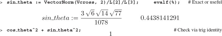
Now we define two symbolic vectors and take their cross product to check that it agrees with the definition of cross product. After that, we form the cross product of our two numeric vectors, vec2 and vec3, and check that it is perpendicular to both of them (and thus to their plane):

We also know that the cross product has a length equal to the product of the lengths of vec2 and vec3 times the sine of the angle between them. So let us compute sin(θ) and see if it agrees with the cos(θ) we computed from the dot product:
7.5.5 Vector Calculus*
Vector calculus may appear a little advanced for beginners, but you will have it here when needed. Because the LinearAlgebra package does not have all of the vector calculus commands of the linalg package, we sometimes must intermix the two packages. To illustrate, invoking Curl just returns its name, which means that the LinearAlgebra package does not know what it means. Hence, we use the linalg[curl] from the linalg package (with the derivatives taken with respect to the second argument):
![]()

7.5.6 Eigenvalues and Eigenvectors*
The command Eigenvectors solves the eigenvalue problem for matrix A:
![]()
That is, Eigenvectors searches for a set of eigenvectors [X] and corresponding eigenvalues [λ] for which (7.28) holds. The eigenvectors are numbered by the index i, where
![]()
with D the dimension of the space spanned by the eigenvectors. As we shall see, the eigenvectors of A are returned as a matrix with vectors as columns, and so some manipulation is required to extract individual eigenvectors:


This particular eigenvalue problem is a degenerate situation in which two of the eigenvalues are equal, and so we do not expect the degenerate eigenvectors to be orthogonal. (Because the matrix A is not Hermitian, we have no guarantee of orthogonality). We will check if they are orthogonal, and then use the Gram-Schmidt orthogonalization procedure to make them orthogonal:

These same matrix calculations are possible with symbolic matrix elements, although this usually take more time, as the matrices get bigger. As we see below, even with matrices, we sometimes have to coerce Maple into distributing the multiplication and then expanding the products so the answer looks the way we want it to:


As is true for other Maple calculations, if any one of the numbers in matrix A contains a decimal point, then Maple will interpret this as a request for a floatingpoint calculation. For matrix calculations, using floats means that the eigenvectors and eigenvalues will be computed numerically and that all elements should be of numeric type. If the calculation is really big, then we recommend a compiled language with a scientific matrix library (we do that in Chapter 17). Here is an example using a numerical form of the previous matrix:

7.5.7 Solution of Linear Equations*
A set of simultaneous linear equations may be written in the matrix form
![]()
If we have n equations for n unknowns, then A will be a square matrix of dimension n, b a vector of constants with length n, and X a vector containing the n unknowns we wish to solve for:

The command LinearSolve(A, b) finds the vector X that solves this equation:

If you are solving a problem in which you have n equations in m unknowns, then A will have n rows and m columns. For a solution to exist, this situation requires b to be a vector of dimension n and X a vector of dimension m. If AX = b has no solution, or if Maple cannot find one, then the null sequence NULL is returned. If AX = b has multiple solutions, then Maple will describe the family of solutions parametrically:


Figure 7.4 The angular velocity vector ω in black and the angular momentum vector L in gray. In Maple you can grab and rotate this figure.
7.6 SOLUTION: ROTATING RIGID BODIES
We now apply the Maple linear algebra tools to the barbell problem of Figure 7.1. Seeing that the barbell is rotating means that the geometry of this figure is correct only for one instant of time, or for all times in a reference frame rotating with the barbell. We will use that rotating frame and then transform it to a stationary frame later.
We are told that the angular velocity vector of the barbell ω lies along the z axis, as shown in Figure 7.4. This means that the barbell is rotating about the z axis. Clearly, then, this is a 3-D problem, so we define ω as a 3-D vector Ω with only a z component:

We want to use Maple to evaluate the angular momentum via (7.15), which for a barbell with two masses has the simple form:

This makes sense, since we know that r1 = -r2 from the figure. Rather than have some very long expressions, we proceed in steps and compute the momentum of each particle next using the cross product:

As expected, m1 is moving into the paper (negative y velocity), and m2 is moving out of the paper. We now compute the angular momentum arising from each mass and add the results:
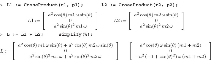
We see that even though the angular velocity is always along the z axis, the angular momentum has an x component, in addition to a z component. Furthermore, since we are viewing the system in a rotating frame, an observer in a fixed frame would see the x component of L rotate (precess) continuously about a fixed z component.
To visualize this solution, we need to assign numerical values to the masses, lengths, angular velocity, and angles:

We now have variables to plot that are numbers and not symbols.
7.6.1 Visualization of Vectors with arrow
Often it is valuable to view a vector as an arrow in space. Maple has the neat command arrow that does just that:

So we now have visualizations of both L and Ω that may be grabbed and rotated. We place them on the same graph by assigning objects to each arrow and then displaying the objects together:

Observe that when we created the arrows we gave some options to the arrow command to control the color and shape of the arrows (use Help arrow for other properties of arrows that can be controlled). We have chosen to make Ω black as a way to indicate that it does not move in time (you are free to grab it and move it as you please, however). Notwithstanding the limited number of options available for the arrow command, the display command permits the usual ones possible for 2-D and 3-D plots (see Chapter 4). For this reason, it is with the display command that we placed labels, titles, and constraints on the scaling so that the vertical and horizontal sizes are true.
Now we would like to convey the notion that the angular momentum vector L is rotating about the Ω vector (which is fixed along the z axis). We do that by creating vectors with the components that L would acquire as it rotates without changing magnitude, and then displaying them all in one plot along with Ω:

7.6.2 Moment of Inertia for the Barbell
We have just evaluated the angular momentum of the barbell by using the elementary definition of angular momentum for each individual mass, and then adding up the two angular momenta. Even though it is possible to follow this approach for any rigid object, it is easier to get the angular momentum by just multiplying the angular velocity ω by the inertia tensor:
![]()
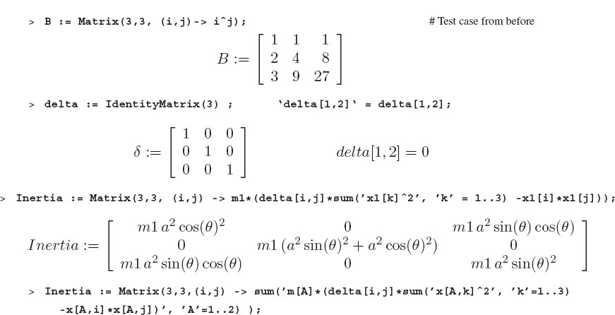
However, to do that we must first evaluate the inertia tensor for the object under study. We start with the basic definition and apply it to the barbell

where the sum over a is over the two masses, and i, j, and k take on the values x, y, and z. The x’s in this equation describe the location of the two masses in Figure 7.1 in terms of Cartesian coordinates (what we called r1 and r2 before):
![]()

The angular velocity vector and the positions of the masses are now known. In order to apply the equation for the moment of inertia, we see that x has subscripts indicating both the mass it corresponds to and its component along the x and y axes. Accordingly, we form a matrix x that has two indices:

To keep this treatment simple, we will explicitly write out the a index over particles and have Maple sum over i and j as subscripts. We start by determining the contribution of mass 1 to the moment of inertia:

To simplify this, we assign the numerical values we had before for the masses, lengths, angular velocity, and angles:
7.7 EXPLORATION: PRINCIPAL AXES OF ROTATION*
We have seen that when the inertia tensor contains off-diagonal elements (products of inertia), the angular momentum and angular velocity of a spinning body are not parallel to each other. It would clearly be simpler if we did not have those offdiagonal elements to deal with. In general, what is “simpler” in life depends upon one’s view of the world, and the inertia tensor is no different. If we rotate the coordinate system we use to calculate the moment of inertia (still keeping it fixed to the body at the center of mass), then it is usually possible to find an orientation for which the inertia tensor is diagonal. In terms of individual elements, a diagonal matrix is expressed as:
![]()
In terms of the matrix representation, this is:

where we are using (1, 2, 3) to label the (x, y, z) axes in this new system. The set of axes in which the inertia tensor becomes diagonal is called the principal axes of inertia.
Finding the principal-axes of inertia is not hard. The whole idea is that the physical angular momentum vector does not change when we choose to view it from different coordinate systems. Therefore when we take the expressions for L in the two systems and set them equal, we obtain equations that Maple will solve for us.
We assume that in the principal-axes system, the body is rotating along one of the principal axes, namely, along the 1, 2, or 3 directions. Then the angular momentum L and the angular velocity ω will be parallel,
![]()
where I is the moment of inertia along the principal axis of rotation (which we cannot yet calculate since we do not know where those axes point). Yet L is still the same vector we expressed previously in (7.17)–(7.19) in terms of the products and moments of inertia. By setting the two expressions equal we obtain three simultaneous linear equations for the unknowns I and ω:

We write these three equations in the matrix form:

The trivial solution is ω = 0. For a nontrivial solution to exist, the matrix on the LHS of this equation must have no inverse. This requires that the determinant of the matrix vanish:

![]()
When the determinant is expanded (something we dare you to try), we are left with a cubic equation in I. The three solutions of this cubic are the three principal moments of inertia, Ix, Iy, and Iz. Once these I’s are known, they are substituted back into the matrix equation to determine the angular momenta via:
We enter the inertia tensor for a cube given as part of the Problem:

Now we form a diagonal matrix with the value Iprin along the diagonal:
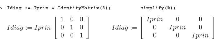
Next we form the matrix whose determinant must vanish. We build the matrix up explicitly from its elements:

Now we calculate the determinant of this matrix and ask Maple to solve for the value of Iprin for which the determinant vanishes:

We should see three principal moments, two of which are equal (a consequence of symmetry). The inertia tensor in the principal-axes frame is thus diagonal:

Although we cannot derive it all here, the indicial equation that we have deduced above is the same one that arises in the eigenvalue problem. For our problem, the eigenvalues are principal moments of inertia, and the eigenvectors are three values for the angular velocity vector ω. Because each eigenvector is associated with one eigenvalue, the principal moment of inertia, the eigenvectors correspond to values of ω for which L and ω are parallel. This causes the directions of the eigenvectors to be the same as the directions of the principal axes in space. To verify this for our cube problem:

We see that Maple first returns a column vector with the same three values of the eigenvalues as we found above. The matrix contains the corresponding three eigenvectors as its columns. Here we separate off the eigenvalues and vectors:


We see that the third eigenvalue corresponds to rotations along the diagonal of the cube, while the first two are perpendicular to the diagonal. To actually visualize these eigenvectors, we represent them as arrows with Maple’s arrow command:

Next, as before, we represent the three omega’s as objects and display them together:


7.8 KEY WORDS AND CONCEPTS
angular momentum |
angular velocity |
columns & rows |
determinant |
diagonalization* |
dot product |
eigenvalues* |
eigenvectors* |
inertia tensor |
linear algebra |
linear equations |
inverse matrix |
matrix arithmetic |
moment of inertia |
polar coordinates |
rigid rotation |
vector |
scalar multiplication |
vector components |
vector magnitude |
vector direction |
2. Is a row vector a matrix?
3. Is a column vector also a matrix?
4. What is the difference between a row and a column vector?
5. Why is the study of matrices and vectors also called linear algebra?
6. How many coordinates are needed to locate a point in space?
7. What meaning is there to a vector having more than three components?
8. Can you add, subtract, and multiply matrices?
9. Can you divide matrices?
10. How are eigenvalues and eigenvectors related?
11. What is the relation between simultaneous equations and matrix equations?
7.9 SUPPLEMENTARY EXERCISES
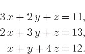
1. Use Maple’s linear algebra commands to find the solution of the simultaneous equations:
2. Find the inverse of the matrix:

3. Verify that the inverse A-1 found in question 2 works in both directions; that is, that
![]()
4. For the same matrix A as in problem 2, find and verify the solution of:

5. In quantum mechanics, the electron’s spin is represented by the three Pauli matrices:

Many of the properties of angular momenta follow from the properties of these matrices.
a. Enter these three matrices into Maple.
b. Use Maple to show that
![]()
c. Use Maple to show that
![]()
d. Use Maple to show that for (i, j, k) in cyclic order namely, [(1, 2, 3), (2, 3, 1), (3, 1, 2)],
![]()
e. Use Maple to show the trace of each of these matrices vanishes,
![]()
6. (You do not have to understand the physics here to do this problem.) Consider a hydrogen atom in a magnetic field B that points in the y direction. If the electron within the atom is described by the Pauli matrices of problem 5, then the Hamiltonian matrix for this system is a Hermitian matrix of the form:

where I is the imaginary number and h is the energy of the atom when there is no magnetic field.
a. The energy of this system is the eigenvalues of this Hamiltonian matrix. Find an analytic expression for the two possible energies for an electron in a magnetic field; namely, find the two eigenvalues of this matrix.
b. Determine the corresponding eigenvectors and show that they are complex yet orthogonal to each other. (Orthogonality is a consequence of the matrix being Hermitian).
7. Determine the relation between the angular momentum and the angular velocities of a uniform plate and cube. Compare that relation to the one we worked out for a plate and cube composed of discrete masses.
8. Consider the matrix:

Solve for the complex eigenvalues and eigenvectors of this matrix. Hint: your eigenvalues should be λ = α-β, λ = α+Iβ.
9. In quantum mechanics, a spin 1 particle is described with the three 3×3 matrices:
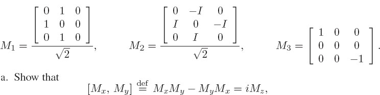
as well as for cyclic permutations of the indices, namely, for index orders yzx and zxy.
![]()
where 1 is the 3-D identity matrix.
1At times the largest value an index assumes is called the dimension of the array, while at other times the number of indices is called the dimension of the array. So, be careful! We call the number of indices the dimension.