
Chapter Nineteen
Discrete Math, Arrays as Bins; Nonlinear Bug Dynamics*
This chapter gives an example of how computations are used to model the population dynamics of biological systems. It employs some fairly simple discrete mathematics that leads to some unusual nonlinear behaviors to explore. One-dimensional arrays are used to bin store the results of the simulations, with the arrays then written to a file and visualized with PtPlot. This chapter introduces no new Java tools, but instead reviews a number of previously introduced techniques. So even though there is no advanced material in it, we mark this chapter as optional since it may be skipped without interrupting the logical flow.
19.1 PROBLEM: VARIABILITY OF BUG POPULATIONS
As is true with much in nature, insect populations do not appear to follow any simple patterns. At times they appear stable, at other times they vary periodically, and at still other times they appear chaotic, only to settle down to something simple again.1
Problem: Deduce and explore a simple model of the population as a function of time that seems capable of producing complicated behaviors.
19.2 THEORY: SELF-LIMITING GROWTH, DISCRETE MAPS
Imagine a bunch of insects reproducing, generation after generation, in your garden. We start with N0 of them, in the next generation we have to live with N1 bugs, and after i generations there are Nn of them to bug us. We want a model for how Nn varies with the discrete generation number n.
We look to the simple model of radioactive decay and growth for guidance.
There we know that an exponential time dependence,
![]()
follows from the simple discrete law [CP 05]:
![]()
Here λ is a rate constant, Nn is the number of particles present in generation n, and Δt is the time for one generation. The model states that the change in the number of particles in one generation is proportional to the number of particles present and to the length of that generation.
We know that a discrete equation such as (19.2) produces growth or decay for positive or negative values of λ respectively, but not both. If bugs just bred, then an exponential-growth model might make sense; yet bugs cannot live on love alone. As their numbers grow the bugs start running out of food and this leads to their numbers growing only to some maximum value N*. We modify the simple growth model by introducing a growth rate λ that decreases as the population number reaches some maximum:
![]()
We expect that when Nn is small compared to the maximum N*, the bugs will grow exponentially, but as Nn becomes comparable in magnitude to N*, the growth rate should decrease and possibly become negative if it exceeds N*.
To make the mathematics of this model clearer, we change to dimensionless variables

In terms of these, our model assumes the simple form
![]()
Here xn is essentially the fraction of the maximum population attained in generation n, and µ is a constant we call the survival rate. The range of variation of these dimensionless parameters are limited to:
![]()
Notwithstanding the simplicity of (19.5) with its one variable x and one parameter µ, it leads to surprisingly complicated behaviors. This is a consequence of its being a nonlinear equation in which the variable x occurs to the second power. It is called the logistics map [Rash 90], and your problem is now reduced to exploring the properties of (19.5).
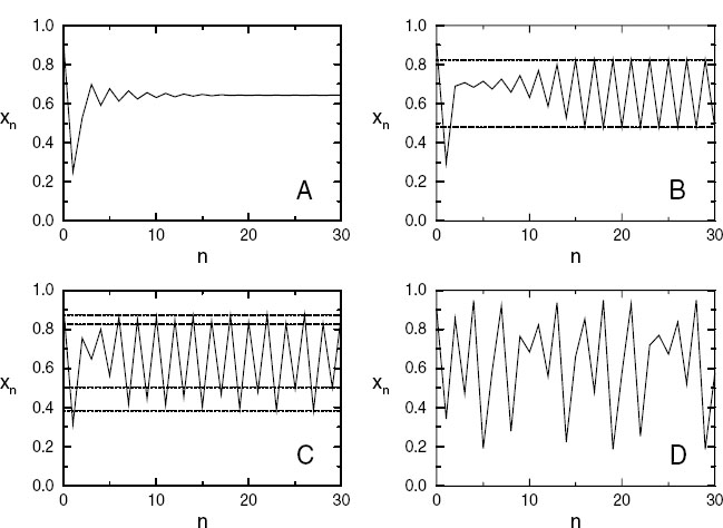
Figure 19.1 The insect population xn versus generation number n for various survival rates: (A) µ = 2.8, a period-one cycle; (B) µ = 3.3, a period-two cycle; (C) µ = 3.5, a period-four cycle; (D) µ = 3.8, a chaotic regime.
19.3 ASSESSMENT: PROPERTIES OF NONLINEAR MAPS
Rather than do some fancy mathematical analysis [Rash 90] to determine properties of the logistics map (19.5), study it directly on the computer. Write a simple program that uses the logistics map to produce a sequence of population values xn as a function of the generation number n. Start with a seed population xQ = 0.75 and plot up xn versus n for µ = (0.4, 2.8, 3.3, 3.5, 3.8). The last four simulations should yield results similar to those in Figure 19.1.
Explore other nearby values of µ and identify on printed copies of your graphs the following characteristics:
Transients: Irregular behaviors before reaching a steady state.
Extinction: If the survival rate is too low, the population dies off.
Stable states: Single-population stable states for µ< 3.
Two and three cycles: At two-cycle fixed points, the population jumps back and forth between two semistable x* values. At three-cycle fixed points the population jumps between three x∗ values. These attractors occur only for µ> 3.
Intermittency: Try to find solutions for 3.8264 < µ < 3.8304 in which the system appears stable for a while but then jumps all around, only to become stable again.
Chaos: The system’s behavior in the chaotic region is critically dependent on the exact value of µ and x 0. Systems may start out much the same but end up quite different. Compare the long-term behaviors of starting with the two essentially identical seeds:
![]()
where e ~ 2 × 10-14 for a double-precision calculation. Repeat the experiment with x0 = 0.75, but with what should essentially be two identical survival parameters:
![]()
19.4 EXPLORATION: BIFURCATION DIAGRAM, BUGSORT.JAVA*
Listing 19.1 BugSort.java


Figure 19.2 The bifurcation plot, attractor populations versus survival rate, for the logistics map.
Listing 19.1 gives our basic program for producing a bifurcation diagram. Computing and watching the population change with each generation gives a good idea of the basic phenomena. However, it is hard to discern the simple and beautiful behavior that lies within these complicated behaviors. One way to gain such understanding is to concentrate on the semistable population values ,x* that the system jumps among over time. These are called attractors to indicate that the system is somehow attracted to these populations.
A plot of these attractors as a function of the survival parameter μ is an elegant way to summarize the results of extensive computer simulations. One such bifurcation diagram is given in Figure 19.2. It shows the output from the program BugSorted.java given here. For each value of μ, hundreds of iterations were made to make sure that all transients died out. The value of x that the system settled down to is recorded as x*. The doublet of points (μ, x*) that occur after the transients have died out were then written to a file. To be sure that all attractors have been reached, the calculation is repeated for various values for the initial populations X0.
19.4.1 Implementation: Bifurcation Diagram
Create your own version of Figure 19.2. To get an idea of how many points may be needed, let us assume that your screen resolution is ~100 dots per inch and that your laser printer’s resolution is ~300 dots per inch. This means that you are plotting approximately 3000 × 3000 10 million elements. Beware: this will take a long time to print and require more memory than some printers have available.
19.4.2 Binning
1. Break up the range 1 < µ < 4 into 1,000 steps and loop through them. These are the “bins” into which we will place the x* values.
2. In order not to miss any structures in your bifurcation diagram, loop through a range of initial x0 values as well.
3. Wait at least 200 generations for the transients to die out, and then print out the next several hundred values of (µ, x*) to a file.
4. Print out your x* values to no more than three to four decimal places. You will not be able to resolve more places than this on your plot, and this will keep your output files smaller by permitting you to remove duplicates. It is hard to control the number of decimal places in output with Java’s standard print commands. However, you may use the Java version of fprintf to do this and sort the file to remove duplicates.2 Another approach is to remove two successive xn values that differ only beyond the third place. We do that in the sample code BugsSorted.java by taking advantage of the fact that xn is in the range
![]()
For this reason, before we write out to a file, we multiply our xn’s by 1,000, cast them as integers, and compare with the previous xn:
![]()
If this condition is met, then we know the xn value differs in the first three decimal places from the previous xn value.
5. Plot up your file of x∗ versus µ. Use small symbols for the points and do not connect them.
6. Enlarge sections of your plot and notice that a similar bifurcation diagram tends to be contained within portions of the original (this is called self-similarity).
7. Look over the series of bifurcations occurring at
![]()
The end of this series is a region of chaotic behavior.
8. Inspect the way this and other sequences begin and then end in chaos. The changes sometimes occur quickly over a very short range of µ, and so you may have to make plots over a very small range of µ values to see the structures.
Table 19.1 Maps for generating xn sequences and bifurcation plots.
Name |
f(x) |
Logistics |
µx(1 — x) |
Tent |
µ(1 — 2x — 1/2) |
Ecology |
xeμ(1 —x) |
Quartic |
µ[1 — (2x — 1)4] |
9. Close examination of Figure 19.2 shows regions where a very large number of populations suddenly change to very few populations with a slight increase in µ. Whereas these may appear to be artifacts of the video display, this is a real effect and these regions are called windows. Check that at µ = 3.828427, chaos turns into a three-cycle population.
19.5 EXPLORATION: OTHER DISCRETE MAPS*
Only nonlinear systems exhibit unusual behavior like chaos. Yet systems are nonlinear in any number of ways. Table 19.1 maps that you may use to generate xn sequences and bifurcation plots.
1We actually use chaos as a technical term meaning complicated behavior in which there does not appear to be any order, but in which there is some simple mathematical description [CP 05].
2For example, with the Unix command sort -u.