Chapter Fourteen
Numerical Integration, Nested Loops, Methods; Power and Energy Usage
In this chapter we explore how computers evaluate integrals numerically. We look at the same energy problem solved with Maple in Chapter 6, where numerical integration also had to be used. This chapter provides a fundamental technique for computational science and a better understanding of calculus. We also gain experience with nested loops, multiple methods, and plotting.
14.1 PROBLEM (SAME AS CHAPTER 6): POWER AND ENERGY
In Chapter 6 we modeled the electrical power use P(t) over time by some simple functions. For example,
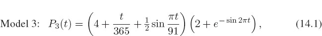
where the power is in GW (109 watts) and the time t is in days (the top curve in Figure 14.1). Your problem is to determine the total energy used over 1000 days (approximately three years) by evaluating the integral

for Model 3, the one that cannot be done analytically.
The highly oscillatory patterns in Figure 14.1 make (14.2) a challenging integral to evaluate (as demonstrated by the quite different answers obtain by casual application of Maple and Mathematica). Consequently, we want you to compare the results from the two different integration rules (trapezoid and Simpson), and to see if the value for the integral converges as we improve the approximations. There are fancier integration rules, but we leave those to the references [Press 94, CP 05].
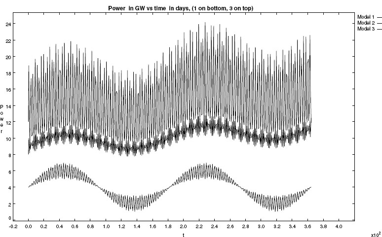
Figure 14.1 Three models of power consumption. The time is in 100 days and the power is in gigawatts.
14.2 ALGORITHMS: TRAPEZOID AND SIMPSON’S RULES
Consider Figure 14.2 showing an arbitrary function f(x) in the interval a ≤ x ≤ b. The definite integral of this function,
is equal to the area under the curve. A traditional way to measure this area is to plot the integrand on a piece of graph paper and add up the number of little boxes lying below the curve. Seeing that boxes are “quadrilaterals,” numerical integration is also called numerical quadrature, even when it gets beyond the explicit box-counting stage.
Numerical-integration techniques usually break the total interval up into small columns, as also shown in Figure 14.2, and then use different approximations to determine the area of each column. When the areas of all the columns are added together, we obtain an approximation for the integral as a weighted sum over the integrand f(x) evaluated at points within the integration region:

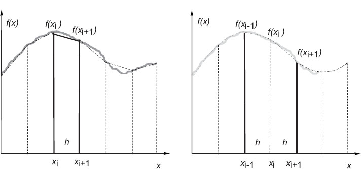
Figure 14.2 Left: Straight-line sections used for the trapezoid rule. An individual trapezoid with area h2 [f(xi) + f(xi+1)] is highlighted. Right: Parabolas used in Simpson’s rule (a single parabola is fit to each pair of consecutive intervals).
Here the xis are integration points and the wis are integration weights. This is a handy way to program up an integration algorithm, since we need only change the specific values for wi (and maybe xi) for different rules.
As the number of integration points N is made progressively larger (narrower columns used), the sum in (14.4) should become a progressively better approximation to the integral. However, if too many points are used, then round-off error tends to accumulate and the approximation stops converging to the exact answer. Consequently, the best integration rules are those which obtain the desired level of precision with the least number of points.
14.2.1 Trapezoid Rule
The trapezoid rule is the simplest integration algorithm. As shown on the left of Figure 14.2, we divide the area under f(x) into a series of columns each of width h, and form trapezoids by approximating the integrand f(x) by a straight line connecting the endpoints of each interval. In this case the integral is approximately equal to the sum of the areas of the columns.1 The approximation gets progressively better as the widths of the trapezoids are made progressively smaller, and the integrand is better approximated by a straight line within the interval.
We first deduce an equation that gives the x value for each integration point.
If we evaluate the function at N points, then we have N -1 columns (it takes two points to define one column) covering the range b–a. It follows then that the width of each interval in Figure 14.2 is

and the discrete x values. They are thus enumerated with the subscript i:
![]()
To calculate the area of each trapezoid in Figure 14.2, we look at the isolated column i. The area of this one trapezoid is its width times its average height:

which is the same area one gets if each column is considered as a rectangle with the top passing through the midpoint of the slanted top. The total area in the integration region from a to b is the sum of the areas of all the columns:

Observe that because each internal point gets counted twice, it gets weighted by h, whereas the endpoints get counted just once and so are weighted by only h/2. In terms of the notation of our standard integration rule (14.4), the points and weights for the trapezoid rule are:


Listing 14.1 Trap.java
14.2.1.1 Implementation: Trap/TrapMethods.java
In Listing 14.1 we give you the Java program Trap.java that uses the trapezoid rule to evaluate the integral of J0 t 2 dt. This is a simple class with only a main method. In Listing 14.2 we give the program TrapMethods.java that does the same integration using two methods. If you find this use of methods easy to follow, then use TrapMethods.java. Otherwise, start with Trap.java and work your way up to TrapMethods.java. In both cases the limits of integration A and B and the number of integration points N are declared as constant (final) class variables before the main method. Being final means that they cannot be changed by assignment statements, while being class variables means that are available to all methods within the class without having to be passed as arguments. In contrast, the variables that actually vary, sum, h, t and w, are declared in main and have to be passed to the methods as needed.
Listing 14.2 TrapMethods.java

Good programming is often modular; that is, composed of a number of small subprograms (methods) each of which accomplishes a single, well-defined task. Listing 14.2 gives TrapMethods.java, a version of our trapezoid-rule integration program that uses two methods. Observe how on line 13 there is the sum over the weighted integrand calling the method f(x), while on line 16 that method is defined as f(y). As we have said before, this is fine as long as the argument types
are the same. If you look next at line 23 you will notice that the value of the weight w is the returned value of the function wTrap(i,h), while i and h are passed to the method as arguments. In contrast, the value of N is used on line 21 but not passed to the method since it is a global, class variable.
1. Compile and execute Trap.java or TrapMethods.java.
2. Modify it to determine the energy usage∫0 P3(t)dt for Model 3.
3. Incorporate the necessary PtPlot statements in your program to produce a plot of Model 3’s P(t) for 1000 days, in steps of 0.5 days. §11.1 describes the use of PtPlot and gives a sample program whose commands may be incorporated in your program.
4. Make a crude graphical estimate (25% accuracy) of the area under your P3(t) vs. t curve. Use 10-day column widths, and count the number of boxes in each column (count fractionally filled boxes as full if they are more than half full), or calculate the area of each trapezoid. Make your boxes big so that you do not have too much work to do, and make sure you have the right units (energy = GW-days) for your choice of boxes.
5. Compare the answer for the integral from your program using 10-day widths with that found from your graph. Do they agree within experimental error?
14.2.1.2 Implementation with Nested Loops
Our approximation to the area under a curve as the sum of columns with straight or rounded tops should get more accurate as we increase the number of columns N-1. However, if we make N too large, then round-off error accumulates to the point where increasing N further leads to a less accurate answer. To get a feel for how accurate our numerical integration technique is, we want to increase N and see in what decimal place the answer changes. If the answer changes in, say, the fourth decimal place, then we would expect the answer to be good to at least three places.
Modify a copy of TrapMethods.java so that it prints out the value of the integral and the value for eight values in the range 25 ≤ N ≤ 200. Rather than run the program eight times, modify the program so that it loops over eight values of N:
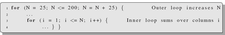
The procedure outlined in this code fragment uses nested loops, namely, one for loop contained within another for loop. Study how for each value of the total number of points N, everything within the outer loop gets repeated, and this includes the inner loop’s i-summation over the areas of each column. Consequently, it is important to check that the program reinitializes the value of the variables used in the inner loop, in particular, h and sum. If you look at line 8 of the TrapMethods.java, you will notice that the column width h varies with the number of integration points used N. Because of that, we need to begin the for loop before line 8. Next notice that the summation over column areas is ended by the right brace on line 15. As a consequence, we need to end the loop over N after line 15.
14.2.2 Improved Method: Simpson’s Rule
Simpson’s rule for integration will also give us an algorithm of the form (14.4), but with different weights than the trapezoid rule. The integration range is again divided into equal-width columns, with the points given by (14.6). Now, as we show on the right of Figure 14.2, we approximate f(x) at the top of every two columns as a parabola:
![]()
This is a better than using a straight line. With each parabola containing three unknown parameters, α, β, and γ, we need three values of f(x) to determine them. We do that by having one parabola pass through the tops of two adjacent columns. Whereas the determination of these constants requires some algebra, the idea is simple. What is important is that because parabolas are being fit to successive pairs of columns, Simpson’s rule requires an odd number of integration points N so that there will be an even number of columns.
14.2.2.1 Simpson’s Rule Weights*
After approximating the integrand f(x) by a parabola in (14.10), it is easy to calculate the area of two columns:

However, to make an algorithm out of this we need to express the parameters α, β, and γ in terms of the values of the integrand within the intervals. To do that we evaluate the integrand f(x) at the three integration points (xi-1 = 0, xi = h, xi+1 = 2h) and solve for the parameters in terms of them:
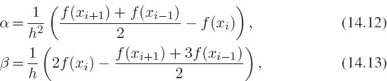
![]()
This leads to the elementary Simpson rule for the area of two columns:

When we apply Simpson’s rule to the entire column, the endpoints of each two-column section get counted twice, since they belong to two different pairs. Yet the first and last endpoints only get counted once:
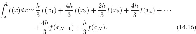
In terms of the notation of our standard integration rule (14.4), Simpson’s rule is:

where the sequence repeatedly alternates between 4h/3 and 2h/3, except for the endpoints. Remember, N must be odd!
14.3 ASSESSMENT: WHICH RULE IS BETTER?
1. Modify your trapezoid-rule program so it prints out running values for the sum, the integrand, the weight, and the loop counter i in equation (14.4)’s notation. By “running values” we mean the value of a variable as it actually changes during the calculation. Looking at these values and checking that they change in the way expected is one of the best ways to ensure that your program is working correctly.
2. Modify a copy of your program so it evaluates the integral using Simpson’s rule. Make the program smart enough to use only an odd number of points for Simpson’s rule. Hint: You test if an integer j is even by testing if 2* (j/2) = j or if j % 2 = 0. The first test takes advantage of the fact that integer arithmetic rounds down, while the second test uses a Java method to determine if the remainder is 0 after division by 2.
3. The numerical approximation for integration should improve as the number of points N increases. Make a table or plot showing the level of accuracy obtained for the integral for various numbers of points:
4. Make a plot of the energy consumption versus time, like that in Figure 14.3, only here for Model 3. How does that compare to the Maple results?
N-1 |
I (trapezoid) |
I (Simpson) |
8 |
- |
- |
: |
||
512 |
- |
- |
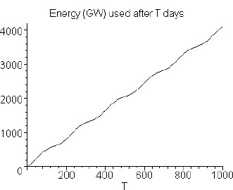
Figure 14.3 Energy consumption as a function of time for model 1 computed with Maple.
14.4 KEY WORDS AND CONCEPTS
integration integration points integration weights modular programs
nested loops quadrature Simpson’s rule trapezoid rule
1. Explain succinctly the difference between the trapezoid and Simpson rules.
2. Is a parabola or a straight line a better approximation for a function?
14.5 SUPPLEMENTARY EXERCISES
1. You are given nonrepeated weights of 1, 2, 4, 8, 16, and 32 kg. Your boss claims that you should be able to use these six weights to weigh any rice sack weighing an integer number of kilograms between 1 and 63. For instance, 63 = 1+2+4+8+16+32. Write a program to check if the claim is true. The program should write the sack weight and the weights used.
2. As a more challenging version of the above problem, imagine that you are given a sack of rice of undermined integer weight less than 64 kg. Write a program that determines the sack’s weight and the individual weights you used to determine it.
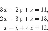
3. The Chinese scholar Sun Tsu in the year 400 BCE found solutions to the problem:
find an integer such that if divided by 3 the residue is 2, if divided by 5 the residue is 3, and if divided by 7 the residue is 2.
Write a program that finds the numbers less that 500 that satisfy these three conditions.
(These three problems come via courtesy of M. Páez.)
1 An alternative way of viewing the trapezoid rule is as forming a series of rectangles with horizontal tops, the height of each rectangle being (fi + fi+1)/2. If we use fi as the height, then we have a version of the trapezoid rule known as Euler’s rule.