Chapter Sixteen

Object-Oriented Programming, Abstract Data; Complex Currents

Note to the instructor: As an alternative to the full version of this chapter, you may skip the study of the RLC circuit and just focus on the mathematics of complex numbers and their representation in terms of objects. And even with that, you may defer the use of nonstatic (object-oriented) methods to a later time.

16.1 PROBLEM: RESONANCE IN RLC CIRCUIT

We are given the circuit shown on the left of Figure 16.1 containing a resistor of resistance R, an inductor of inductance L, and a capacitor of capacitance C. All three elements are connected in series to an alternating voltage source

Problem: Determine the magnitude and time dependence of the current in this RLC circuit as a function of the frequency of the external voltage. We will solve the RLC circuit problem for you within this chapter. Your problem is to repeat the calculation for a circuit in which there are two RLC circuits in parallel, as shown on the right of Figure 16.1. You may assume a single value for inductance and capacitance, and three values for resistance:

Consider frequencies of applied voltage in the range 0 < ω < 2 √LC = 2/s.

16.2 MATH: COMPLEX NUMBERS

Try to remember your first exposure to square roots in elementary school. Though it was straightforward to understand that 5 ² = 25, it was a challenge to understand that /25 = ±5, and more of a challenge to understand what was the true value of p24. For many of us, it was downright impossible to understand the true value of /—1. Mathematicians, being a rather clever and proud bunch, have handled this affront to their abilities by inventing the number i as the answer,¹

Figure 16.1 Left: An RLC circuit connected to an alternating voltage source. Right: Two R L C circuits connected in parallel to an alternating voltage. Observe that one of the parallel circuits has double the values of R, L, and C as does the other.

where the “def” over the equal sign indicates a definition. In this way mathematicians have a way of going ahead with their calculations, even if they do not know what i means. Whereas defining away one’s ignorance may appear to be a swindle, mathematicians are an honest bunch at heart and so tell the world that they have really just made up the answer by calling i the imaginary number. “Imaginary” is a good name for i, since there is no way to measure this number in the real world, but, then again, there is no law forbidding us from imagining such a number.

In common mathematical usage, i is called the imaginary number, while any multiple of i is called an imaginary number. So, for example, 2i, i, and 100i are all imaginary numbers. Once we have extended our minds to imagine an imaginary number, it is not much of a stretch to imagine adding a real number to an imaginary number to form something more complex. To name an instance, 1 + i, 1 + 2i, and 100 + 76i. These numbers with both real and imaginary parts are called complex numbers.² The term “complex” indicates that these numbers have a number of parts, and not that they are hard to understand!

Complex numbers are very useful in mathematics and science since they let us double our work output with only the slightest increase in input. This is accomplished by employing the familiar operations of algebra and calculus on complex numbers, and then separating off the real and imaginary parts of the answer at the end. By way of example, even if z is a complex number, z³/z still equal z², without our having to express the individual numbers in terms of their real and imaginary parts.

Figure 16.2 Representation of a complex number as a vector in space.

To do algebra with complex numbers, we define the symbol z to represent a number with both real and imaginary parts:

In turn, the complex nature of z is indicated by giving its real and imaginary parts:

In a strict sense, y is the magnitude of the imaginary part of z, and iy is the imaginary part. Yet y is usually called “the imaginary part.”

Because complex numbers have independent real and imaginary parts, a useful way to visualize them is to imagine a coordinate system in which the ordinate points off into imaginary space and the abscissa points off into real space. As seen in Figure 16.2, we then visualize z = x +iy as a point with y projection along the imaginary axis and x projection along the real axis. This is analogous to a vector in a 2-D space, except that part of this vector lies in an imaginary space. The analogy between complex numbers and 2-D vectors is taken one step further by applying the polar coordinate representation of a vector to complex numbers. On account of this, the point z in Figure 16.2 may be located not only by giving its Cartesian coordinates x and y, but also by specifying it polar coordinates r, the length of the vector from the origin to point z, and θ, the angle that the vector makes with the abscissa. The complex number is the same in either case, and, indeed, the two representations are related via simple trigonometry:

16.2.1 Complex Arithmetic Review

The essence of the computing aspect of our problem is the programming of the rules of arithmetic for complex numbers. This is an interesting chore because while Java contains all the rules for real numbers, you must educate Java as to the rules for complex numbers. Indeed, since complex numbers are not primitive data types like doubles and floats, we will construct complex numbers as objects.³

We start with two complex numbers, which we distinguish with subscripts:

The rules of arithmetic follow by applying algebra to the real and imaginary parts:

In deducing the rule for complex division we employed the fact that a complex number z multiplied by its complex conjugate

We observe that this result is the same as the square of the length r defined in (16.6). The length r is commonly referred to as the modulus or magnitude of the complex number z, and is expressed by using the absolute value symbol: r = |z|. The product of the complex number z and its complex conjugate z∗ is then

Exercise: Consider the complex numbers

What are the values of b+c, b—c, b×c, |c|, and b/c? ♠

We end our little review with an examination of functions of complex numbers. The new idea here is an ingenious theorem, derived by Euler, that if you raise e, the base of the natural logarithm system, to a purely imaginary power, then you get a complex number with a sine and cosine as its real and imaginary parts:

If the angle θ is real and in radians, then cos θ and sin θ are identified with the projection of exp iθ along the real and imaginary axes, respectively. So if we look at both Figure 16.2 and Eqs. (16.4) and (16.6), we see that it is also possible to express a complex number z in terms of its polar representation:

An important application of Euler’s theorem is to define what it means to raise a number to a complex power z, for example,

We shall find (16.19) useful in our exercises.

16.3 THEORY: RESISTANCE BECOMES IMPEDANCE

The basic rules of circuit theory are called Kirchoff’s laws [R & M 93], and we now apply one of them to the circuit on the left of Figure 16.1. We work our way around the circuit, setting the external voltage V (t) equal to the sum of the voltage drops across the resistor, the inductor, and the capacitor. If I(t) is the current in the circuit, we end up with the basic differential equation of circuit theory

where we have taken an extra derivative to eliminate an integral. The solution to our problem follows by solving (16.20) when the voltage has the form V (t) = V₀ cos ωt. An elegant way to do that is to recognize that

Because (16.20) is a linear equation (only first power of I occurs), the law of linear superposition holds. This means that if we imagine the circuit being driven by a complex voltage source, whose real part is the physical voltage, then the resulting current I(t) will also be complex, with its real part the physical current. Thus we assume that the current has the form

If we substitute this and the complex V (t) into (16.20), we obtain

Here Z is called the impedance and is the complex expression

Equation (16.23) is the generalization of Ohm’s law, V = IR, to alternating current circuits.⁴ We see that the real part of the impedance is just the resistance R, while the imaginary part (called the reactance) is 1/ωC – ωL. As we shall see, the imaginary part of the impedance determines the phase of the current.

16.3.1 Solution for Complex Current

If we now solve (16.23) for the complex current, we obtain

Eq. (16.25) is more illuminating if the complex impedance is expressed in polar form:

We see now that the complex current is

which means that the physical current is its real part:

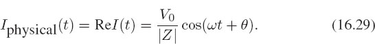
Equation (16.29) states that the amplitude of the current in the circuit is given by the amplitude of the voltage divided by the magnitude of the complex impedance, and that the phase of the current, relative to that of the voltage, is given by θ. If the phase θ>0, then the current leads the voltage in time, that is, the current reaches its maximum before the voltage reaches its maximum. If θ is negative, then the current lags the voltage.

Finally, what is to be done if we have two such RLC circuits in parallel, as shown on the right of Figure 16.1. The analysis is the same as that done with ordinary resistors. If two impedances are in series, then they have the same current passing through them. If two impedances are in parallel, then they have the same voltage across them. If two impedances are connected in series, then the voltages add, and this leads to:

Figure 16.3 An abstract drawing, or what?

If the impedances are connected in parallel, then the currents add, and this leads to

Hence in the parallel case, the impedances add in inverse, with all the steps of the calculation being performed with complex arithmetic.

16.4 CS: ABSTRACT DATA TYPES, OBJECTS

What do you see when you look at the abstract object in Figure 16.3? Some readers may see a face in profile, others may see some parts of human anatomy, and others the total absence of artistic ability. This figure is abstract in the sense that it does not try to present a true or realistic picture of the object, but rather uses a symbol to suggest more than meets the eye.

Abstract or formal concepts pervade mathematics and science because they make it easier to describe nature. For example, we often use the symbol v(t) to denote the velocity of an object as a function of time. Despite velocity being a familiar concept, it is actually abstract in the sense that we cannot see it. What we see is the position of the object as a function of time, and then we infer from that the velocity by determining how rapidly that position is changing.

In computer science we create an abstract object by using a symbol to describe a collection of items. We have already seen that data, or variables in Java and Maple may be integers, floating-point numbers, Booleans, or strings. These types of variables are built into the languages and therefore are called primitive data types. In addition, computer languages let the user define abstract data types of their own by combining primitive data types into more complicated structures called objects. These objects are abstract in the sense that they are named with a single symbol, yet they represent a number of parts.

For instance, one might create an object with parts that contain a student’s school record (ID, grades, etc.), as well as other parts that contain methods to calculate the grade point average, etc. Of course, one would need many such objects because there are many students. To distinguish between the general structure of this student-record object and specific record objects for individual students, the general object is called a class, while the object for specific cases is called an instance of the class, or just an object.

In this chapter our objects will be complex numbers, while in other chapters they may be plots, vectors, or matrices. The classes that we form will be combinations of abstract data types and associated methods for modifying those data. The entire class may also be thought of as objects. In a formal sense, computer science requires abstract data types to possess the three properties [Zach 96]:

Typename: procedure to construct the new data type from elementary pieces.

Set values: mechanism for assigning values to the defined data type.

Set operations: rules that permit operations on the new data type (you would not have gone to all the trouble of declaring a new data type unless you were interested in doing something with it).

In terms of these properties, when we declare a variable to be complex we satisfy property (1). When we declare Rez=x and Imz =y as doubles, we satisfy (2). When we define the rules of arithmetic and trigonometry for complex numbers (as reviewed in § 16.2.1), we satisfy (3).

Before we examine how these properties are applied in our programs, let us review the structure we have been using in our Java programs. When we start off our programs with a declaration statement such as double x. This tells the Java compiler the kind of variable x is, so that Java will store it properly in memory and use proper operations on it. The general rule is that every variable we use in a program must have its data type declared. For primitive (built-in) data types, we declare them to be double, float, int, char, long, short, or boolean.

If our program employs some user-defined, abstract data types, then they too must be declared. This declaration must occur even if we do not define the meaning of the data type until later in the program (the compiler checks on that). Consequently, when our program refers to a number z as complex, the compiler must be told at some point that there is both a real part x and an imaginary part y that makes up a complex number.

To actually create objects in your Java program, you need class variables and methods that are nonstatic. This means we leave off the word static in declaring the class and variables. If the class and class variables are no longer static they may be thought of as dynamic. Likewise, methods that deal with objects may be either static or dynamic. The static ones take objects as arguments, much like conventional mathematical functions. In contrast, dynamic methods accomplish the same end by modifying or interacting with the objects. Regardless of our starting our dealings with objects using static methods, you must use dynamic (nonstatic) methods to enjoy the full power of object-oriented programming.

16.4.1 Object Declaration and Construction

Before we start working with objects in a program, it is necessary to understand that even though we may assign a name like x to an object, because objects have multiple components, you do not assign one explicit value to the object. It follows then, that when Java deals with objects it does so by reference. In plain English this means that the name of the variable refers to the location in memory where your object is stored, and not to the explicit values of the object’s parts. To see what this means in practise, the class file Complex.java in Listing 16.1 adds and multiplies complex numbers, with the complex numbers represented as objects.

Exercise: 1. Enter the program Complex.java by hand, trying to understand it as best you are able. (Yes, we know that you can just copy it, but then you do not become familiar with the constructs.)

2.  Study how the word Complex is a number of things in this program. It is the name of the class (line 2), as well as the name of two methods that create the object (lines 7 and 11). Methods, such as these, that create objects are called constructors. In spite of neophytes viewing these multiple uses of the name Complex as confusing (Landau’s second rule), more experienced users often view it as elegant and efficient. Look closely and take note that this program has nonstatic variables (no static on line 3).

3.  Compile and execute this program, and check that the output agrees with the results you obtained in the exercises in §16.2.1.     ♠

The first thing to notice about Complex.java is that the class is declared on line 2 with the statement

The main method is declared on line 23 with the statement

These are the same techniques we have employed before (it is good when some things stay the same in life). However, on line 3 we see that the variables re and im are declared for the entire class with the statement

Listing 16.1 Complex.java

Although this is similar to the declaration we have seen before for class variables, observe that the word static is absent. This indicates that these variables are interactive or dynamic, namely, parts of an object. They are dynamic in the sense that they will be different for each object (instance of the class) created. That is, if we define z1 and z2 to be Complex objects, then the variables re and im will be different for z1 and z2.

We extract the component parts of our complex object by a projection operation. For those readers who know some vector analysis, think of this as similar to extracting the components of a vector in space by taking dot products with the unit vectors to project the vector onto different axes. As with space vectors, the projection operation is denoted by a dot operation:

This same dot convention is used to access the methods of objects, as we will see below. On line 4 we see a method Complex declared with the statement

On line 7 we see a method Complex declared, yet again, but with a somewhat different statement:

Some explanation is clearly in order! First notice that both of these methods are nonstatic (no word static). In fact, they are the methods that construct our complex number object, which we call Complex. Second notice that the name of each of these methods is the same as the name of the class, Complex.⁵ Indeed, you know that they are special since by convention they are spelled with their first letters capitalized, rather than the lowercase letters usually used for methods, and because these objects have the same name as the class they are in.

The two Complex methods are used to construct the object, and for this reason are called constructors. The first Complex constructor on line 4 is seen to be a method that takes no argument and returns no value (yes, this appears rather weird, but be patient). When Complex gets called with no argument, as we see on line 25, the real and imaginary parts of the complex number (object) are set to zero. This method is called the default constructor, since it does what Java would otherwise do automatically (“by default”) when first creating an object, namely, set all of its component parts initially to zero. We have explicitly included it for pedagogical purposes.

Exercise: Remove the default constructor (the one on line 4 that takes no argument) from Complex.java and check that you get the same result for the call to Complex().     ♠

The Complex method on line 7 implements the standard way to construct complex numbers. It is seen to take the two doubles x and y as input arguments, to set the real part of the complex number (object) to x, the imaginary part to y, and then return. This method is an additional constructor for complex numbers but differs from the default constructor by taking arguments. Inasmuch as the nondefault constructor takes arguments while the default constructor does not, Java does not confuse it with the default constructor, even though both methods have the same name.

Okay, let us now take stock of what we have up to this point. On line 3 Complex.java has defined the variables re and im that will be the two separate parts of the created object. As each instance of each object created will have different values for the object’s parts, these variables are referred to as instance variables. Because the name of the class file and the names of the objects it creates are all the same, it sometimes is useful to use yet another word to distinguish one from the other. Hence the phrase instance of a class is used to refer to the created objects (in our example, a, b, and c). This distinguishes them from the definition of the abstract data type.

Now let us look at the main method to see how to go about creating objects using the constructor Complex. On line 24, in the usual place for declaring variables, we have the statement

Because the compiler knows that Complex is not one of its primitive (built-in) data types, it assumes that it must be one we have defined. In the present case, the class file contains the nonstatic class named Complex, as well as the constructors for Complex objects (data types). This means that the compiler does not have to look very far to know what you mean by a complex data type. By reason of this, when the statement Complex a, b; on line 24 declares the variables a and b to be Complex objects, we know that they are manifestly objects since the constructors are not static.

Recall that declaring a variable type, such as double or int, does not assign a value to the variable, but, instead, tells the compiler to add the name of the variable to the list of variables it will encounter. Likewise, the declaration statement Complex a, b lets the compiler know what type of variables these are without assigning values to their parts. To actually create objects we have to place numerical values in the memory locations that have been reserved for them. Seeing that an object has multiple parts, we cannot give all its parts initial values with a simple assignment statement like a = 0;, so something fancier is called for. This is exactly why the constructor methods are used. Specifically, on line 25 we have the object a created with the statement

and on line 26 we have the object b created with the statement

Look at how the creation of a new object requires the command new to precede the name of the constructor (Complex in this case). Also note that line 25 uses the default constructor method to set both the re and im parts of a to zero, while line 26 uses the second constructor method to set the re part of b to 4.7 and the im part of b to 3.2.

Just as we have done with the primitive data types of Java, it is possible to both declare and initialize an object in one statement. Indeed, line 27 does just that for object c with the statement

Monitor how the data type Complex precedes the variable name c in line 27 because the variable c has not previously been declared; future uses of c should not declare or create it again.

16.4.2 Static and Nonstatic Methods

Once our complex-number objects have been declared (added to the variable list) and created (assigned values), it is easy to do arithmetic with them. For those readers seeing objects for the first time, we suggest that you get some experience with object arithmetic using the familiar static methods that we have been using up until now. That is what we do in this section. In the next section §16.4.2.1, which we consider optional for object neophytes, we show how to perform the same object arithmetic using nonstatic methods. Undeniably, nonstatic methods are elegant and powerful; however, they do their work in a different way and so may take some getting used to before making sense. We recommend that even the object neophytes read §16.4.2.1 before getting on to the exercises. After that it should be possible to make more sense out of the nonstatic methods and even to repeat the exercises using nonstatic methods (an approach we encourage).

We have now declared and created objects that represent complex numbers.

We know from §16.2.1 all the rules of complex arithmetic and complex trigonometry, so next we will write Java methods to implement these rules. It makes sense to place these methods in the same class file that defines the data type since these associated methods are needed to manipulate objects of that data type. This is an interesting task since it is analogous to the one faced by those people who originally wrote the Java language and had to program up all the methods to do arithmetic with real numbers.

On line 30 in our main program we see the statement

This statement says to add the complex number b to the complex number c and then to store the result “as” (in the memory location reserved for) the complex number a. You may recall that we initially set the re and im parts of a to zero in line 25 using the default Complex constructor. This statement will replace the initial zero values with those computed in line 30. Nevertheless, it often helps the debugging process to have zero initial values.

The method add that adds two complex numbers is defined on lines 11–15. It starts with the statement

The method is declared to be static and takes as its input arguments the two Complex objects (numbers) a and b. The fact that the word Complex precedes the method’s name add signifies that the method will return a Complex number object as its result. We had the option of defining other names like Complex_add or plus for this addition method, but we opted to keep things simple instead.

The calculational part of the add method starts on line 12 by declaring and creating a temporary Complex number temp that will contain the result of the addition of the Complex numbers a and b. As indicated before, the dot operator convention with objects means that temp.re will contain the re part of temp and that temp.im will contain the imaginary part. Thus the statements on lines 13 and 14,

add the Complex numbers a and b by extracting the real parts of each, adding them together, and then storing the result as the re part of temp. Line 20 determines the imaginary part of the sum in an analogous manner. Finally, the statement

returns the object (Complex number) temp as the value of add(Complex a, Complex b). Because a Complex number has two parts, both parts must be returned to the calling program, and this is what return temp does.

16.4.2.1 Nonstatic Methods*

In this section we present a nonstatic approach for dealing with Complex objects. If you have just read the section on static methods for dealing with objects and feel somewhat confused by it, we recommend that you jump ahead to the exercises to get some experience with the more elementary aspects of objects before using the nonstatic methods described here. Then come back here to see what nonstatic methods are all about.

The program ComplexDyn.java in Listing 16.2 at the end of this section also adds and multiplies Complex numbers as objects, but it uses what are called dynamic, nonstatic, or interactive methods. This is more elegant and powerful, but less like the procedural programming we have been doing up till now. To avoid confusion and to permit you to run both the static and nonstatic versions without them interfering with each other, the nonstatic version is called ComplexDyn, in contrast to the Complex used for the static method. Inspect how the names of the methods in ComplexDyn and Complex are the same, although they go about their work differently.

Exercise: 1. Enter the ComplexDyn.java class file by hand, trying to understand it in the process. If you have entered Complex.java by hand, you may modify that program to save some time (but be careful!).

2.  Compile and execute this program, and check that the output agrees with the results you obtained in the exercises in §16.2.1.     ♠

Nonstatic methods go about their work by modifying the properties of the objects to which they are attached (for the present case the objects are Complex numbers). In fact, we shall see that nonstatic methods are literally appended to the name of objects much as the endings of verbs are modified when their tenses change. In other words, the method gets appended to the object and in so doing becomes part of the object. To cite an instance, on line 27 we see the operation

Study the way this statement says to take the Complex number object c and modify it using the add method that adds b to the object. This results in new values for the parts of object c. Because object c gets modified by this action, line 27 is equivalent to the static operation

Regardless of the approach, since c now contains the sum c+b, if we want to use c again we must redefine it, as we do on line 30. On line 31 we take object c and multiply it by b with,

This method changes c to c*b. Thus line 31 has the static-method equivalence

We see from these two examples that nonstatic methods are called using the same dot operator that is used to refer to instance variables of an object. On the other hand, static methods take the object as arguments and do not use the dot operator. Thus we called the static methods using add(c,b) and mult(c,b) and called the nonstatic methods using c.add(b) and c.mult(b).

The static methods here do not need a dot operator, since they are called from within the class Complex or ComplexDyn that defined them. However, they would need a dot operator if called from another class. As an instance, you have already seen what we called the method Math.sqrt(x). This is actually the static method sqrt from the class Math. You could call the static add(c,b) method of class Complex by using Complex.add(c,b). This works within Complex as well, but is not required. It is required, however, if add is called from other classes.

Observe now how the object-oriented add method has the distinctive form:

Line 11 tells us that the method add is nonstatic (the word static is absent), that no value or object is returned (the void), and that there is one argument other of the type ComplexDyn. What is clearly unusual about this nonstatic method is that it is supposed to add two Complex numbers together, yet there is only one argument given to the method and no object returned! Indeed, the assumption is that since the method is nonstatic, it will only be used to modify the object that called it. Hence it “goes without saying” that there is an object around for this method to modify, and the this reference is used to refer to “this” calling object. In fact, the reason the argument to the method is conventionally called other, is to distinguish it from the this object that the method will modify. (We are being verbose for clarity’s sake: the word “this” may be left out of these statements without changing their actions.) Consequently, when the object addition is done in line 12 with

it is understood that re will refer to the current object being modified (this), while other will refer to the “other” object that is being used to make the modifications.

Listing 16.2 ComplexDyn.java

16.5 JAVA SOLUTION: Complex CURRENTS

1.  Extend the class Complex.java or ComplexDyn.java by adding new methods to subtract, take the modulus, take the Complex conjugate, and determine the phase of Complex numbers.

2.  Test your methods by checking that the following identities hold for a variety of Complex numbers: Hint: Compare your output to some cases of pure real, pure imaginary, and simple Complex numbers that you are able to evaluate by hand.

3. Equations (16.29) and (16.27) are the solution for the current in a single RLC circuit. It tells us that the magnitude of the current is given by

and that the phase of the current (relative to the cos ωt time dependence) is

Modify the given Complex arithmetic program so that it performs the Complex arithmetic required by (16.33). Hint: You do not have to solve this from scratch! Instead, use the techniques you have already programmed for determining the magnitude to determine |I|.

4.  Compute and then make a plot of the magnitude and the phase of the current in the circuit as a function of frequency ω of the external voltage source. For our problem, a good range is 0 < ω < 2.

5.  Assessment: You should notice a resonance peak in the magnitude at the same frequency for which the phase vanishes. The smaller the resistance R, the sharper should the circuit pass through resonance. These types of circuits were used in the early days of radio to tune to a specific frequency. The sharper the peak, the better the quality of reception.

6.  The second part of the problem dealing with the two circuits in parallel is very similar to the first part. You need to change only the value of the impedance Z used. To do that, explicitly perform the Complex arithmetic implied by (16.31), deduce a new value for the impedance, and then repeat the calculation of the current.

16.6 MAPLE SOLUTION: Complex CURRENTS

Recall from way back in Chapter 3 that Maple knows all about Complex numbers and Complex arithmetic. Indeed, you have probably already seen an occasional I pop up as the solution to some equations. The point here is that Maple reserves the symbol I as the /—1, and this lets us use its I at our pleasure:

In §16.3 we applied circuit theory and Complex analysis to the RLC circuit and found that if the exciting voltage is the real part of then the current in the circuit is

Here Z is the Complex impedance,

We will start our Maple investigation by trying to determine magnitude |Z| and phase θ of Z using Maple’s capabilities for Complex analysis. Whereas needing to know the magnitude and phase of Z is just another way of saying that we need to know Z in polar notation, we have Maple calculate these for us:

This is just a fancy way of giving us back the input. The problem is that Maple does not know that ω, R, L, and C are real, and so it cannot do the Complex arithmetic. To tell Maple that the constants are real, we tell it what to assume:

It has taken some work, but now we are ready for some Complex arithmetic. Look at the polar form:

This is giving us the correct magnitude, but Maple appears unable to compute the phase. This seems to be a Maple failure. However, we get it to work by combining the map and evalc commands:

Here map applies the procedure evalc to each element of polar(Z) and returns the polar form (|Z|, θ). This simplifies the elements into the form needed. [It should not be this hard!] We get separate expressions out for the real and imaginary parts by using the command op(numb,expression) to extract the numb-th operand from expression:

The expressions we have just derived are the standard ones for the magnitude and the phase of the impedance Z. However, since the current is proportional to 1/|Z|, we will plot 1/|Z|. We could compute 1/Z and work with that as well.

16.6.1 Maple’s Surface Plots of Complex Impedance

We want to examine the current that occurs in the RLC circuit as a function of the driving frequency. We have already discussed in Chapter 4 some of Maple’s commands for plotting Complex functions. Irrespective of them being illuminating, for the problem given here, we first use plot3d to make the familiar z(x, y) surface plot of the magnitude and phase of the current as functions of both the frequency of the external voltage ω and of the resistance R:

Check o√ut how the magnitude has a maximum when the external frequency ω = 1/ LC. This is the resonance frequency. For our choice of constants this corresponds to ω= 1. We now make some plots to see if this is true.

Sure enough, the plot of 1/|Z| shows that the magnitude of the current has a maximum at ω= 1. (It helps to grab and rotate these plots to see them better.) We also see that as the resistance R in the circuit is made smaller, the maximum current becomes progressively larger. The second plot of the phase shows that below resonance, ω<1, the current lags the voltage, while above resonance the current leads the voltage. Another way to visualize Complex functions is with the command Complexplot3d. It makes a 3-D visualization of a Complex function of a Complex argument. Here we do it by treating the frequency ω = x+iy as a Complex number:

We see in the right plot above that there is a sharp peak at x = Re(ω) = 1, as expected. The color change indicates where Im(1/Z ) changes sign. If we look closely at this graph we will also see that there is a maximum for a negative imaginary value of ω. This is related to how long the resonance stays excited, a statement we do not try to prove here.

Figure 16.4 Superposition of two waves with similar wave numbers (a PtPlot).

16.7 EXPLORATIONS: OOP WORKED EXAMPLES*

Creating object-oriented programs (OOP) requires a transition from a procedural-programming mindset in which functions take arguments as input and produce answers as output, to one in which objects are created, probed, transferred, and modified. To assist you in the transition, we present here (courtesy of Manuel Páez) two sample procedural programs and their OOP counterparts. In both cases the OOP examples are longer but presumably easier to modify and extend.

16.7.1 OOP Beats

Listing 16.3 Beats.java

First-year physics [Ser 00] usually explains how you obtain beats if you add together two sine functions y₁ and y₂ with nearly identical frequencies,

As shown in Figure 16.4, beats look like a single sine wave with a slowly varying amplitude. In Listing 16.3 we give Beats.java, a simple program that plot beats.

You see here that all the computation is done in the main program, with no methods called other than those for plotting. On lines 13 and 14 the variables y1 and y2 are defined as the appropriate functions of time, and then added together on line 15 to form the beats. Contrast this with the object-oriented program OOPBeats.java in Listing 16.4 that produces the same graph.

Listing 16.4 OOPBeats.java

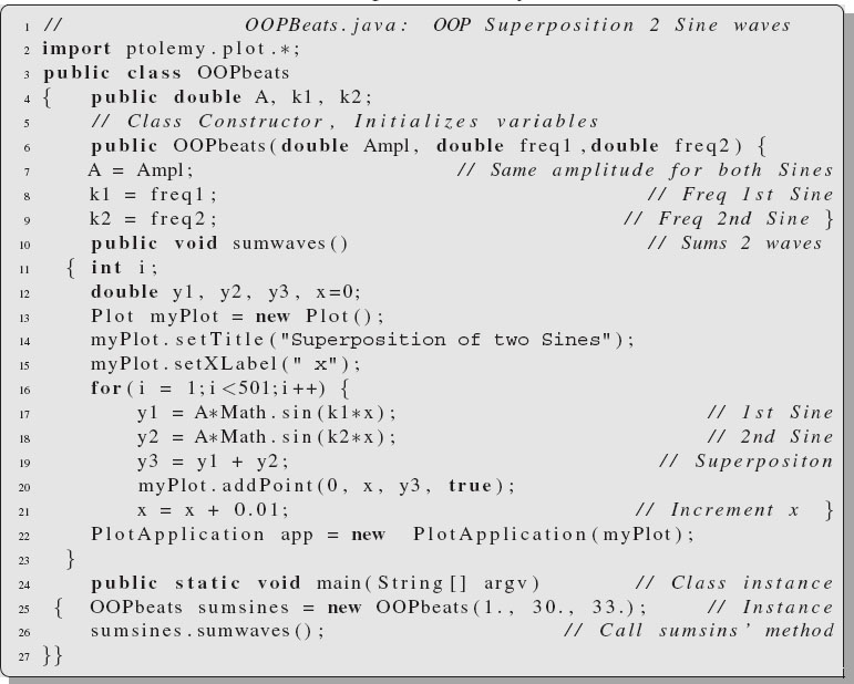
Here the main program is at the very end, on lines 24–27. It is short because all it does is create an OOPbeats object named sumsines on line 25 with the appropriate parameters and then, on line 26, sums the two waves by having the method sumwaves modify the object. The constructor for an OOPbeats object is given on line 6, with the sumwaves method given on line 10. The sumwaves method takes no arguments and returns no value; the waves are summed on line 19 and the graph plotted all within the method.

Figure 16.5 The trajectory of a satellite as seen from the sun.

16.7.2 OOP Planet

Listing 16.5 Moon.java

In our second example we add together periodic functions representing positions versus time. One set describes the position of the moon as it revolves around a planet, and the other set describes the position of the planet as it revolves about the sun. Specifically, the planet orbits the sun at a radius R=4 units with an angular frequency ωp =1 radian/sec, while the moon orbits the Earth at a radius r=1 unit from the planet and an angular velocity ωs = 14 radians/sec. In mathematical terms, the position of the planet at time t relative to the sun is described by

The position of the satellite, relative to the sun, is given by sums of its position relative to the planet, plus the position of the planet relative to the sun:

So again this looks like beating (if ωs — ωp, and if we plot x or y versus t), except now we will make a parametric plot Ofx(t) versus y(t) to obtain a visualization of the orbit.

A procedural program Moon.java to do this summation and to produce the visualization shown in Figure 16.5 is in Listing 16.5.

Exercise: Rewrite the program using OOP.

1.  Define a mother class OOPlanet containing:

Radius planet’s orbit radius

wplanet planet’s orbit ω

(xp, yp) planet coordinates

(getX(double time), getY(double time) methods for planet coordinates

trajectory() method for planet’s orbit

2.  Define a daughter class OOPMoon containing:

radius radius of moon’s orbit

wmoon frequency of moon in orbit

(xm, ym) moon coordinates

trajectory() method for moon’s orbit relative to sun

3.  The main program must contain one instance of the class planet and another instance of the class Moon, that is, one planet object and one Moon object.

4.  Have each instance call its own trajectory method to plot the appropriate orbit. For the planet this should be a circle, while for the moon it should be a circle with retrogrades, as shown in Figure 16.5.     ♠

One solution, which produces the same results as the previous program, is our program OOPlanet.java in Listing 16.6. As with OOPbeats.java, the main program for OOPlanet.java is at the end, on line 56. It is short since all it does is create an OOPMoon object on line 68 with the appropriate parameters, and then have the moon’s orbit plotted by applying the trajectory method to the object on line 69.

Listing 16.6 OOPPlanet.java

What is new about this program is that it contains two classes, OOPlanet beginning on line 3, and OOPMoon beginning on line 39. This means that when you compile the program you should obtain two class files, OOPlanet.class and OOPMoon.class. Yet since execution begins in the main method, and the only main method is in OOPMoon, you need to execute OOPMoon.class to run the program:

Scan the code to see how the class OOPMoon is within the class OOPlanet, and is therefore a subclass. Accordingly, OOPMoon is called a daughter class and OOPlanet is called a mother class. The daughter class inherits the properties of the mother class, as well as having properties of its own. Thus, on lines 51–52 OOPMoon uses the getX(time) and getY(time) methods from the OOPlanet class, without having to say OOPlanet.getX(time) to specify the class name.

16.8 KEY WORDS

abstract data types	reactance	frequency	imaginary number
Complex conjugate	constructor	current	default constructor
Complex arithmetic	class	impedance	instance of object
instance variable	magnitude	modulus	nonstatic methods
nonstatic variable	object	voltage	polar representation
Complex number	reference call	resonance	user-defined data types
object creation

16.9 JAVA AND MAPLE EXERCISES

1The invention is credited to Girolama Cardana (1501–1576).

2The term, as well as much in applied mathematics, is credited to Carl Friedrich Gauss (1777–1855).

3Because Complex numbers are used so often in science and engineering, there is a move afoot to have some future versions of Java incorporate Complex numbers as a primitive data type in order to speed up execution and make them easier to use.

4Some elementary texts may refer to |Z| as the impedance and then use the concept of phasors to describe the effect of the impedance on the phase. We view the use of Complex impedance as more direct and elegant.

5These two nonstatic methods are special as they permit the parameters characterizing the object that they construct to be passed during a new call. However, you probably will not understand this statement until we describe the new call.