Chapter Six

Integration; Power and Energy Usage (Also 14)

6.1 PROBLEM: RELATING POWER AND ENERGY USAGE

The use of electrical power is characterized by variations of different sorts. There are fluctuations related to the day-night cycle, fluctuations related to the change of seasons (approximately monthly), fluctuations due to weather patterns (daily and long-term), and others [Energy]. As an instance, observe the hourly use of power for Australia during a one-year period shown in Figure 6.1 [D&A 00]. Generally, power consumption peaks in the winter due to heating demands, and peaks again in the summer due to cooling demands. Power usage also shows a year-to-year growth that may be related to population growth and economic development, as well as the seasonal variation that is the most evident, especially when the daily fluctuations are removed by taking averages over weekly periods.

Problem: Determine the total energy used over a three-year period.

6.2 EMPIRICAL MODELS

The data for power usage is just a series of numbers, each for a different time, and therefore not in an appropriate form for analytic integration.¹ We model it approximately with three formulas:

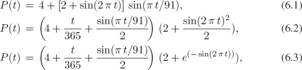
where the power P(t) is in GW (10⁹ watts) and the time t is in days. These formulas try to incorporate the various time dependencies of power usage. Since t is in days, a function of the form sin(2 π t/T) is periodic with period T days. Therefore sin(2 π t) in these models represents a daily variation of power. Likewise, sin(π t/91) has a period of 182 days (half of a year), and so represents a variation that peaks twice during the year. Models 2 and 3 have a term that grows linearly with time to account for year-to-year growth. Finally, model 3 incorporates an exponential time dependence of power use on a daily time scale.

Figure 6.1 Electrical power use for Australia (left) and Mad del Plata (right) on an hourly basis over a one-year period.

To see if these models look anything like the data, we plot them:

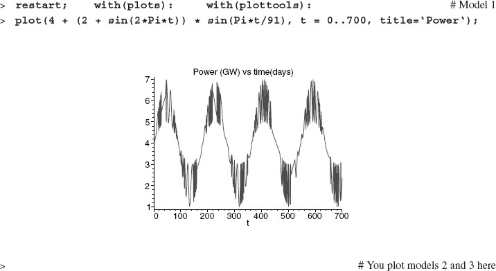
Indeed, there is a biyearly variation about a nonzero average, a daily variation, and, for models 2 and 3, a long-term growth of the average.

6.3 THEORY: POWER AND ENERGY DEFINITIONS

In common usage, the words “power” and “energy” may differ from their scientific meanings (like paying the “power bill” when you are really buying energy). Power is defined as the rate at which work is done, or energy used:

Consequently, if energy is measured in joules (the System International unit), then power is measured in joules/second or watts (W).

The power company charges you for kilowatt-hours. A kilowatt is 1,000 watts, an hour is 3,600 seconds, and so one kilowatt-hour = 1000 watts × 3600 sec = 3.6 × 10⁶ joules. Typical costs for a kWh is between 2 and 20 cents, depending on where you live and politics. In any case, you are paying for energy, not power. To set the scale for some realistic numbers, one horsepower (hp) equals 746 W. One energy worker, the average output power of a human body, is 100 W, significantly less than a horse. A nuclear power plant produces energy at the rate of 1,150 megawatts, significantly more than a horse.

In our problem we are given the power used as a function of time and asked to compute the energy used in three years. Rearranging the definition of power, (6.4) gives the energy used during infinitesimal time dt as

which gives he total energy used from some time 0 to T as

This means that the solution to our problem is the integration of the three models for power usages, (6.1)–(6.3), which is equivalent to measuring the areas under the P(t) vs. t curves. If an analytic integration is possible, then we will have a function W(T) to use for predicting future energy usage. Otherwise we just have to evaluate the integral numerically and plot the numbers up to see the trends.

6.4 MAPLE: TOOLS FOR INTEGRATION

Integrals were invented to determine quantities such as the potential energy in the interior of a spherical planet:

Calculus is still essential for solving scientific problems, and Maple is good at calculus. In the previous chapter we studied the derivative, here we study the integral, which is essentially the inverse of the derivative (antiderivative). An integral without explicit limits, such as ∫ f(x) dx, is an indefinite integral. An integral with limits, such as ∫_a^b f(x) dx, is a definite integral. The difference is important; an indefinite integral is still a function of x, while a definite integral is just a number. As we are about to see, Maple handles both types of integrals.

6.4.1 Indefinite Integration

The Maple command for integration is int, with inert form Int:

Look at the second argument to int. It is the variable with respect to which we want the integration performed. Be careful, it does not have to be x:

where, we would have to include the integration constant by hand, if needed. We check the answer via differentiation:

Beware, int does not write out a constant of integration for these indefinite integrals. You will need to include that by hand when appropriate.

6.4.2 Definite Integration

Definite integration includes the integration limits as a second argument in the int command:

In spite of Maple’s awesome powers for doing integrals, some functions cannot be integrated analytically:

We see that Maple just repeats the integral without evaluating it. This response is Maple’s way of saying that it is stumped without losing face. However, even if Maple cannot figure out an exact value for the integral, it should be able to evaluate it numerically. To do that, just tell Maple to evaluate with floats (evalf):

Now and then you may have to try different approaches to get a workable form for a needed integral, for example,

Have Maple evaluate this expression for S as an indefinite integral, and then have Maple evaluate this expression for S as the definite integral:

Even the definite integral is terribly complicated. See if substituting some numerical values for the constants helps:

6.4.3 Integrals as Functions

It should be noted that int, like diff, produces an expression, not a function. Use the unapply command to make the indefinite integral I(x) = ∫ f(x) dx into a function of x:

In view of the fact that definite integrals are just numbers, the unapply command does not work for them. However, let us imagine an integral as a function of both its upper and lower integration limits:

The integral clearly depends upon y and z, the endpoints of the interval. Thus we make the integral a function of the endpoints:

6.5 PROBLEM SOLUTION: ENERGY FROM POWER

We now know how to evaluate integrals, so let us do some! We will investigate models 1 and 3 here, and leave model 2 for you. For model 1, let us first define a function for the power, and then look at it to see if it looks OK:

Now that we know that the integrand looks reasonable, let us integrate it:

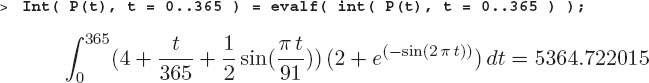
The expression for the integral is neat and shows that the total energy used has some terms that oscillate as a function of time, as well as a term that increases linearly with time. However, it is missing the integration constant, which is clear since the t = 0 value of the integral is –182/π, when it should be 0. One way of eliminating the need to personally include the integration constant, is to evaluate the integral as a definite integral:

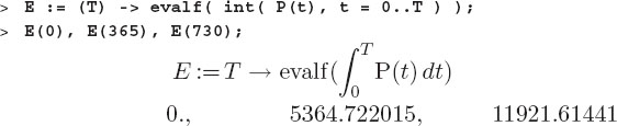
The above equation is not as neat an expression as the indefinite integral, but it is correct (vanishes at T = 0). We define the energy function E(t) as the power integrated up to time T, and evaluate the energy used after one year:

Maple is returning the one-year result as an exact number, which really does not make much sense here, since we want a floating-point number to tell the stockholders. Consequently, we modify the definition of E(t) to float the answer and look at the answers for zero, one, and two years:

The energy used does appear to be growing year by year, something we here check with a simple plot for 1,000 days:

We see a small fluctuation about a linear increase. This does not bode well for the planet!

We now conduct a similar study for model 3. The power function is now:

This model looks good and shows an interesting daily and yearly variation. Now that we know that the integrand looks reasonable, let us integrate it:

Maple appears to give up on us (just repeating the input), so let us try the definite integral form:

Again Maple fails us. Maybe numerical integration works?

Yes that works, so let us define an energy function equal to the integral of the power, and plot and evaluate the results:

This calculation takes some computer time, since Maple must do a numerical integration, and Maple is slow with numerics. In the present case, we have a highly oscillatory integrand and Maple’s adaptive step sizing may have trouble. We are free to try Maple’s plot command, however, since it uses a minimum of 50 points, this also takes a real long time. Consequently, we use the resolution option to set the number of horizontal points to less than the default value of 200:

We see, again, a rather linear increase in energy use for the next few years.

6.5.1 Your Solution to Model 2

6.6 KEY WORDS AND CONCEPTS

definite integral indefinite integral integration constant power vs. energy integration limits

6.7 SUPPLEMENTARY EXERCISES

Evaluate the following integrals:

1In Chapter 14 we do this integration numerically with Java. Numeric integration can be used on tables of numbers as well as functions, and is often required for realistic problems.