
Non-Stationary Signal Analysis Time-Frequency Approach
Ljubiša Stankovi![]() *, Miloš Dakovi
*, Miloš Dakovi![]() * and Thayananthan Thayaparan†, *Electrical Engineering Department, University of Montenegro, Montenegro, †Defense Scientist, Defence R&D, Ottawa, Canada
* and Thayananthan Thayaparan†, *Electrical Engineering Department, University of Montenegro, Montenegro, †Defense Scientist, Defence R&D, Ottawa, Canada
Abstract
Basics of time-frequency signal analysis are presented in this chapter. Linear time-frequency representations, with the short-time Fourier transform, as its most important representative, are overviewed in its first part. Continuous and discrete realizations are presented, along with the discussion of on the implementations and signal reconstruction. The quadratic representations are analyzed next, with the Wigner distribution and its generalizations in the form of Cohen class, being in their core. Higher order time-frequency representations are the topic of the third part of this chapter. The latest results in time-frequency processing of sparse signal in time-frequency domain follow. The presentation in this chapter concludes with list of the selected areas of time-frequency signal analysis applications.
Keywords
Non-stationary signal analysis; Time-frequency signal analysis; Short-time Fourier transform; Wigner distribution; Instantaneous frequency; Higher order time-frequency analysis; Sparse time-frequency signal analysis; Applications of time-frequency signal analysis
3.03.1 Introduction
The Fourier transform (FT) provides a unique mapping of a signal from the time domain to the frequency domain. The frequency domain representation provides the signal’s spectral content. Although the phase characteristic of the FT contains information about the time distribution of the spectral content, it is very difficult to use this information. Therefore, one may say that the FT is practically useless for this purpose, i.e., that the FT does not provide a time distribution of the spectral components.
Depending on problems encountered in practice, various representations have been proposed to analyze non-stationary signals in order to provide time-varying spectral description. The field of the time-frequency signal analysis deals with these representations of non-stationary signals and their properties. Time-frequency representations may roughly be classified as linear, quadratic or higher order representations.
Linear time-frequency representations exhibit linearity, i.e., the representation of a linear combination of signals equals the linear combination of the individual representations. From this class, the most important one is the short-time Fourier transform (STFT) and its variations. A specific form of the STFT was originally introduced by Gabor in mid 1940s. The energetic version of the STFT is called spectrogram. It is the most frequently used tool in time-frequency signal analysis [1–6].
The second class of time-frequency representations are the quadratic ones. The most interesting representations of this class are those which provide a distribution of signal energy in the time-frequency plane. They will be referred to as distributions. The concept of a distribution is borrowed from the probability theory, although there is a fundamental difference. For example, in time-frequency analysis, distributions may take negative values. Other possible domains for quadratic signal representations are the ambiguity domain, the time-lag domain and the frequency-Doppler frequency domain.
Despite the loss of the linearity, the quadratic representations are commonly used due to higher time-frequency concentration compared to linear transforms. A quadratic time-frequency representation known as the Wigner distribution was the first representation introduced in 1932. It is interesting to note that the motivation for definition of this distribution, as well as for some others, was found in quantum mechanics. The Wigner distribution was introduced into the signal theory by Ville in 1948. Therefore, it is often called the Wigner-Ville distribution. In order to reduce undesirable effects, other quadratic time-frequency distributions have been introduced. A general form of all quadratic time-frequency distributions has been defined by Cohen (1966) and introduced in time-frequency analysis by Claasen and Mecklenbräuker (1981). This generalization prompted the introduction of new time-frequency distributions, including the Choi-Williams distribution, Zhao-Atlas Marks distribution and many other distributions referred to as the reduced interference distributions [1,2,6–18].
Higher order representations have been introduced in order to further improve the concentration of time-frequency representations [6,19–22].
3.03.2 Linear signal transforms
A transform is linear if a linear combination of signals is equal to the linear combination of the transforms. Various complex forms of signal representations satisfy this property, starting from the short-time Fourier transform, via local polynomial Fourier transform and wavelet transform, up to general signal decomposition forms, including chirplet transform. Although energetic versions of the linear transforms, calculated as their squared moduli, do not preserve the linearity, they will be considered within this section as well.
3.03.2.1 Short-time fourier transform
The Fourier transform (FT) of a signal ![]() and its inverse are defined by
and its inverse are defined by
![]() (3.1)
(3.1)
![]() (3.2)
(3.2)
The FT of a signal ![]() shifted in time for
shifted in time for ![]() , i.e.,
, i.e., ![]() , is equal to
, is equal to ![]() . The amplitude characteristics of
. The amplitude characteristics of ![]() and
and ![]() are the same and equal to
are the same and equal to ![]() . The same holds for a real valued signal
. The same holds for a real valued signal ![]() and its shifted and reversed version
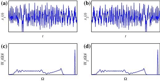
and its shifted and reversed version ![]() . We will illustrate this with two different signals
. We will illustrate this with two different signals ![]() and
and ![]() (distributed over time in a different manner) producing the same amplitude of the FT (see Figure 3.1)
(distributed over time in a different manner) producing the same amplitude of the FT (see Figure 3.1)
 (3.3)
(3.3)
![]()
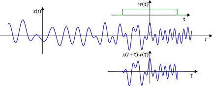
The idea behind the short-time Fourier transform (STFT) is to apply the FT to a portion of the original signal, obtained by introducing a sliding window function ![]() which will localize, truncate (and weight), the analyzed signal
which will localize, truncate (and weight), the analyzed signal ![]() . The FT is calculated for the localized part of the signal. It produces the spectral content of the portion of the analyzed signal within the time interval defined by the width of the window function. The STFT (a time-frequency representation of the signal) is then obtained by sliding the window along the signal. Illustration of the STFT calculation is presented in Figure 3.2.
. The FT is calculated for the localized part of the signal. It produces the spectral content of the portion of the analyzed signal within the time interval defined by the width of the window function. The STFT (a time-frequency representation of the signal) is then obtained by sliding the window along the signal. Illustration of the STFT calculation is presented in Figure 3.2.
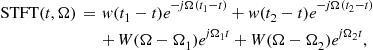
Analytic formulation of the STFT is
![]() (3.4)
(3.4)
From (3.4) it is apparent that the STFT actually represents the FT of a signal ![]() , truncated by the window
, truncated by the window ![]() centered at instant t (see Figure 3.2). From the definition, it is clear that the STFT satisfies properties inherited from the FT (e.g., linearity).
centered at instant t (see Figure 3.2). From the definition, it is clear that the STFT satisfies properties inherited from the FT (e.g., linearity).
By denoting ![]() we can conclude that the STFT is the FT of the signal
we can conclude that the STFT is the FT of the signal ![]() .
.
Another form of the STFT, with the same time-frequency performance, is
![]() (3.5)
(3.5)
where ![]() denotes the conjugated window function.
denotes the conjugated window function.
It is obvious that definitions (3.4) and (3.5) differ only in phase, i.e., ![]() for real valued windows
for real valued windows ![]() . In the sequel we will mainly use the first definition of the STFT [23].
. In the sequel we will mainly use the first definition of the STFT [23].
Example 1
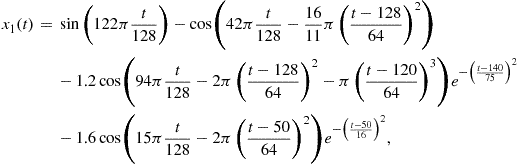
To illustrate the STFT application, let us perform the time-frequency analysis of the following signal:
![]() (3.6)
(3.6)
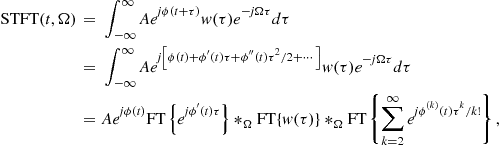
The STFT of this signal equals
 (3.7)
(3.7)
where ![]() is the FT of the used window. The STFT is depicted in Figure 3.3 for various window lengths, along with the ideal representation.
is the FT of the used window. The STFT is depicted in Figure 3.3 for various window lengths, along with the ideal representation.

The STFT can be expressed in terms of the signal’s FT
 (3.8)
(3.8)
where ![]() denotes convolution in
denotes convolution in ![]() . It may be interpreted as an inverse FT of the frequency localized version of
. It may be interpreted as an inverse FT of the frequency localized version of ![]() , with localization window
, with localization window ![]() .
.
3.03.2.1.1 Windows
It is obvious that the window function plays a critical role in the localization of the signal in the time-frequency plane. Thus, we will briefly review windows commonly used for localization of non-stationary signals.
Rectangular window:
The simplest window is the rectangular one, defined by

whose FT is
![]()
The rectangular window function has very strong side lobes in the frequency domain, since the function ![]() converges very slowly as
converges very slowly as ![]() . Thus, in order to enhance signal localization in the frequency domain, other window functions have been introduced.
. Thus, in order to enhance signal localization in the frequency domain, other window functions have been introduced.
Hann(ing) window: This window is of the form
Since ![]() , the FT of this window is related to the FT of the rectangular window of the same width as
, the FT of this window is related to the FT of the rectangular window of the same width as
![]()
Function ![]() decays in frequency much faster than
decays in frequency much faster than ![]() . The previous relation also implies the relationship between the STFTs of the signal
. The previous relation also implies the relationship between the STFTs of the signal ![]() calculated using the rectangular and Hann(ing) windows,
calculated using the rectangular and Hann(ing) windows, ![]() and
and ![]() , given as
, given as
![]() (3.9)
(3.9)
For the Hann(ing) window ![]() of the width
of the width ![]() , in the analysis that follows, we may roughly assume that its FT
, in the analysis that follows, we may roughly assume that its FT ![]() ,is non-zero only within the main lattice
,is non-zero only within the main lattice ![]() , since the side lobes decay very fast. It means that the STFT is non-zero-valued in the shaded regions in Figure 3.3a–c. We see that the duration in time of the STFT of a delta pulse is equal to the widow width
, since the side lobes decay very fast. It means that the STFT is non-zero-valued in the shaded regions in Figure 3.3a–c. We see that the duration in time of the STFT of a delta pulse is equal to the widow width ![]() . The STFTs of two delta pulses
. The STFTs of two delta pulses ![]() and
and ![]() (very short duration signals) do not overlap in time-frequency domain if their distance is greater than the window duration
(very short duration signals) do not overlap in time-frequency domain if their distance is greater than the window duration ![]() . Since the FT of the Hann(ing) window converges fast, we can intuitively assume that a measure of duration in frequency is the width of its main lobe,
. Since the FT of the Hann(ing) window converges fast, we can intuitively assume that a measure of duration in frequency is the width of its main lobe, ![]() . Then, we may say that two (complex) sine waves
. Then, we may say that two (complex) sine waves ![]() and
and ![]() do not overlap in frequency if the condition
do not overlap in frequency if the condition ![]() holds. It is important to observe that the product of the window durations in time and frequency is a constant. In this example, considering time domain duration of the Hann(ing) window and the width of its main lobe in the frequency domain, this product is
holds. It is important to observe that the product of the window durations in time and frequency is a constant. In this example, considering time domain duration of the Hann(ing) window and the width of its main lobe in the frequency domain, this product is ![]() . Therefore, if we improve the resolution in the time domain
. Therefore, if we improve the resolution in the time domain ![]() , by decreasing T, we inherently increase value of
, by decreasing T, we inherently increase value of ![]() in the frequency domain. This essentially prevents us from achieving the ideal resolution in both domains. A general formulation of this principle, stating that product of window durations in time and in frequency cannot be arbitrary small, will be presented later.
in the frequency domain. This essentially prevents us from achieving the ideal resolution in both domains. A general formulation of this principle, stating that product of window durations in time and in frequency cannot be arbitrary small, will be presented later.
Hamming window: This window has the form
Similar relations between the Hamming and the rectangular window transforms hold as in the case of Hann(ing) window. This window has lower first side lobe than the Hann(ing) window. However, since it has a discontinuity at ![]() , its convergence as
, its convergence as ![]() is not faster in frequency than in the case of a Hann(ing) window.
is not faster in frequency than in the case of a Hann(ing) window.
Gaussian window: This window localizes signal in time, although it is not time-limited. Its form is
![]()
In some applications it is crucial that the nearest side lobes are suppressed as much as possible. This is achieved by using windows of more complicated forms, like the Blackman window and the Kaiser window [6].
3.03.2.1.2 Duration measures and uncertainty principle
We started discussion about the signal concentration (window duration) and resolution in the Hann(ing) window case, with illustration in Figure 3.3. In general, window (any signal) duration in time or/and in frequency is not obvious from its definition or form. Then, the effective duration is used as a measure of window (signal) duration. In time domain the effective duration measure is defined by
Similarly, the measure of duration in frequency is

Here, it has been assumed that the time and frequency domain forms of the window (signal) are centered, i.e., ![]() and
and ![]() . If this were not the case, then the widths of centered forms in time and frequency would be calculated.
. If this were not the case, then the widths of centered forms in time and frequency would be calculated.
The uncertainty principle in signal processing states that the product of effective measures of duration in time and frequency, for any function satisfying ![]() as
as ![]() , is
, is
![]() (3.10)
(3.10)
Since this principle will be used in the further analysis, we will present its short proof. Since ![]() is the inverse FT of
is the inverse FT of ![]() , according to the Parseval’s theorem we have
, according to the Parseval’s theorem we have
![]()
and the product ![]() may be written as
may be written as
![]()
where ![]() is the energy of the window (signal),
is the energy of the window (signal),
![]()
For any two integrable functions ![]() and
and ![]() , the Cauchy-Schwartz inequality
, the Cauchy-Schwartz inequality
![]()
holds. The equality holds for
![]()
where ![]() is a positive constant.
is a positive constant.
In our case, the equality holds for
![]()
The finite energy solution of this differential equation, with ![]() , is the Gaussian function
, is the Gaussian function
![]()
For the Gaussian window (signal) it may be shown that this product is equal to ![]() , meaning that the Gaussian window (signal) is the best localized window (signal) in the sense of effective durations. In the sense of illustration in Figure 3.3, this fact also means that, for a given width of the STFT of a pulse
, meaning that the Gaussian window (signal) is the best localized window (signal) in the sense of effective durations. In the sense of illustration in Figure 3.3, this fact also means that, for a given width of the STFT of a pulse ![]() in time direction, the narrowest presentation of a sinusoid in frequency direction is achieved by using the Gaussian window.
in time direction, the narrowest presentation of a sinusoid in frequency direction is achieved by using the Gaussian window.
3.03.2.1.3 Continuous STFT inversion
The original signal ![]() may be easily reconstructed from its STFT (3.4) by applying the inverse FT, i.e.,
may be easily reconstructed from its STFT (3.4) by applying the inverse FT, i.e.,
![]() (3.11)
(3.11)
In this way, we can calculate the values of ![]() for a given instant t (
for a given instant t (![]() ) and for the values of
) and for the values of ![]() where
where ![]() is non-zero. Then, we may skip the window width, take the time instant
is non-zero. Then, we may skip the window width, take the time instant ![]() , and calculate the inverse of
, and calculate the inverse of ![]() , and so on.
, and so on.
Theoretically, for a window of the width ![]() , it is sufficient to know the STFT calculated at
, it is sufficient to know the STFT calculated at ![]() with
with ![]() , in order to reconstruct signal for any t (reconstruction conditions will be discussed in details later, within the discrete forms).
, in order to reconstruct signal for any t (reconstruction conditions will be discussed in details later, within the discrete forms).
A special case for ![]() gives
gives
![]() (3.12)
(3.12)
For the STFT defined by (3.5) the signal can be obtained as
![]()
In order to reconstruct the signal from its STFT, we may skip the window width at t and take as the time instant ![]() . If we calculate
. If we calculate ![]() for all values of t (which is a common case in the analysis of highly non-stationary signals), the inversion results in multiple values of signal for a given instant, which all can be used for better signal reconstruction as follows:
for all values of t (which is a common case in the analysis of highly non-stationary signals), the inversion results in multiple values of signal for a given instant, which all can be used for better signal reconstruction as follows:
![]()
In the case that we are interested only in a part of the time-frequency plane, relation (3.12) can be used for the time-varying signal filtering. The STFT, for a given t, can be modified by ![]() and the filtered signal obtained as
and the filtered signal obtained as
![]()
For example we can use ![]() within the time-frequency region of interest and
within the time-frequency region of interest and ![]() elsewhere.
elsewhere.
The energetic version of the STFT, called the spectrogram, is defined by

Obviously, the linearity property is lost in the spectrogram. The spectrograms of the signals from Figure 3.1 are presented in Figure 3.4.
Figure 3.4 The spectrograms of the signals presented in Figure 3.1.
3.03.2.1.4 STFT of multi-component signals
Let us introduce multi-component signal ![]() as the sum of M components
as the sum of M components ![]() ,
,
 (3.13)
The STFT of this signal is equal to the sum of the STFTs of individual components,
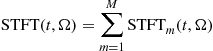 (3.14)
that will be referred to as the auto-terms. This is one of very appealing properties of the STFT, which will be lost in the quadratic and higher order distributions.
The spectrogram of multi-component signal (3.13) is of the form:
only if the STFTs of signal components, ![]() ,
, ![]() , do not overlap in the time-frequency plane, i.e., if
, do not overlap in the time-frequency plane, i.e., if
![]()
In general

where the second term on the right side represents the terms resulting from the interaction between two signal components. They are called cross-terms. The cross-terms are undesirable components, arising due to non-linear structure of the spectrogram. Here, they appear only at the time-frequency points where the auto-terms overlap. We will see that in other quadratic time-frequency representations they may appear even if the components do not overlap.
3.03.2.2 Discrete form and realizations of the STFT
In numerical calculations the integral form of the STFT should be discretized. By sampling the signal with sampling interval ![]() we get
we get

By denoting
![]()
and normalizing the frequency ![]() by
by ![]() , we get the time-discrete form of the STFT as
, we get the time-discrete form of the STFT as
![]() (3.15)
(3.15)
We will use the same notation for continuous-time and discrete-time signals, ![]() and
and ![]() . However, we hope that this will not cause any confusion since we will use different sets of variables, for example t and
. However, we hope that this will not cause any confusion since we will use different sets of variables, for example t and ![]() for continuous time and n and m for discrete time. Also, we hope that the context will be always clear, so that there is no doubt what kind of signal is considered.
for continuous time and n and m for discrete time. Also, we hope that the context will be always clear, so that there is no doubt what kind of signal is considered.
It is important to note that ![]() is periodic in frequency with period
is periodic in frequency with period ![]() . The relation between the analog and the discrete-time form is
. The relation between the analog and the discrete-time form is
![]()
The sampling interval ![]() is related to the period in frequency as
is related to the period in frequency as ![]() . According to the sampling theorem, in order to avoid the overlapping of the STFT periods (aliasing), we should take
. According to the sampling theorem, in order to avoid the overlapping of the STFT periods (aliasing), we should take
![]()
where ![]() is the maximal frequency in the STFT. Strictly speaking, the windowed signal
is the maximal frequency in the STFT. Strictly speaking, the windowed signal ![]() is time limited, thus it is not frequency limited. Theoretically, there is no maximal frequency since the width of the window’s FT is infinite. However, in practice we can always assume that the value of spectral content of
is time limited, thus it is not frequency limited. Theoretically, there is no maximal frequency since the width of the window’s FT is infinite. However, in practice we can always assume that the value of spectral content of ![]() above frequency
above frequency ![]() , i.e., for
, i.e., for ![]() , can be neglected, and that overlapping of the frequency content above
, can be neglected, and that overlapping of the frequency content above ![]() does not degrade the basic frequency period.
does not degrade the basic frequency period.
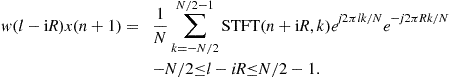
The discretization in frequency should be done by a number of samples greater than or equal to the window length N. If we assume that the number of discrete frequency points is equal to the window length, then
 (3.16)
and it can be efficiently calculated using the fast DFT routines
![]()
for a given instant n. When the DFT routines with indices from 0 to ![]() are used, then a shifted version of
are used, then a shifted version of ![]() should be formed for the calculation for
should be formed for the calculation for ![]() . It is obtained as
. It is obtained as ![]() , since in the DFT calculation periodicity of the signal
, since in the DFT calculation periodicity of the signal ![]() , with period N, is inherently assumed.
, with period N, is inherently assumed.
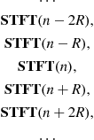
For the rectangular window, the STFT values at an instant n can be calculated recursively from the STFT values at ![]() , as
, as

This recursive formula follows easily from the STFT definition (3.16).
For other window forms, the STFT can be obtained from the STFT obtained by using the rectangular window. For example, according to (3.9) the STFT with Hann(ing) window ![]() is related to the STFT with rectangular window
is related to the STFT with rectangular window ![]() as
as
![]()
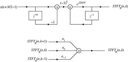
This recursive calculation is important for hardware implementation of the STFT and other related time-frequency representations (e.g., the higher order representations implementations based on the STFT).
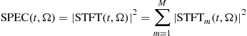
A system for the recursive implementation of the STFT is shown in Figure 3.5. The STFT obtained by using the rectangular window is denoted by ![]() , Figure 3.5, while the values of coefficients are
, Figure 3.5, while the values of coefficients are
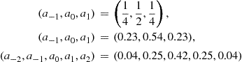
for the Hann(ing), Hamming and Blackman windows, respectively.
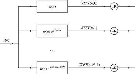
3.03.2.2.1 Filter bank STFT implementation
According to (3.4), the STFT can be written as a convolution
![]()
where an even, real valued, window function is assumed, ![]() . For a discrete set of frequencies
. For a discrete set of frequencies ![]() , and discrete values of signal, we get that the discrete STFT, (3.16), is an output of the filter bank with impulse responses
, and discrete values of signal, we get that the discrete STFT, (3.16), is an output of the filter bank with impulse responses
![]()
what is illustrated in Figure 3.6.
Illustrative example: In order to additionally explain this form of realization, as well as to introduce various possibilities for splitting the whole time-frequency plane, let us assume that the total length of discrete signal ![]() is
is ![]() , where N is the length of the window used for the STFT analysis. If the signal was sampled by
, where N is the length of the window used for the STFT analysis. If the signal was sampled by ![]() , then the time-frequency region of interest in the analog domain is
, then the time-frequency region of interest in the analog domain is ![]() and
and ![]() , with
, with ![]() , or
, or ![]() and
and ![]() in the discrete time domain. For the illustration we will assume
in the discrete time domain. For the illustration we will assume ![]() .
.
The first special case of the STFT is the signal itself (in discrete time domain). This case corresponds to window ![]() . Here, there is no information about the frequency content, since the STFT of one sample
. Here, there is no information about the frequency content, since the STFT of one sample ![]() is the sample itself, i.e.,
is the sample itself, i.e., ![]() , for the whole frequency range. The whole considered time-frequency plane is divided as in Figure 3.7a.
, for the whole frequency range. The whole considered time-frequency plane is divided as in Figure 3.7a.

Figure 3.7 Time-frequency plane for a signal ![]() having 16 samples: (a) The STFT of signal
having 16 samples: (a) The STFT of signal ![]() using one-sample window. (Note that
using one-sample window. (Note that ![]() , for
, for ![]() .) (b) The STFT obtained by using a two-samples window
.) (b) The STFT obtained by using a two-samples window ![]() , without overlapping. (c) The STFT obtained by using a four-samples window
, without overlapping. (c) The STFT obtained by using a four-samples window ![]() , without overlapping. (d) The STFT obtained by using an eight-samples window
, without overlapping. (d) The STFT obtained by using an eight-samples window ![]() , without overlapping. (e) The STFT obtained by using a 16-samples window
, without overlapping. (e) The STFT obtained by using a 16-samples window ![]() , without overlapping. (Note that
, without overlapping. (Note that ![]() for
for ![]() for all n.) (f) The STFT obtained by using a four-samples window
for all n.) (f) The STFT obtained by using a four-samples window ![]() , calculated for each n. Overlapping is present in this case.
, calculated for each n. Overlapping is present in this case.
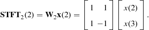
Let us now consider a two samples rectangular window, ![]() , with
, with ![]() . The corresponding two samples STFT is
. The corresponding two samples STFT is
![]()
for ![]() (corresponding to
(corresponding to ![]() ) and
) and
![]()
for ![]() (corresponding to
(corresponding to ![]() ). Thus, the whole frequency interval is represented by the low frequency value
). Thus, the whole frequency interval is represented by the low frequency value ![]() and the high frequency value
and the high frequency value ![]() . From the signal reconstruction point of view, we can skip one sample in the STFT calculation and calculate
. From the signal reconstruction point of view, we can skip one sample in the STFT calculation and calculate ![]() and
and ![]() , and so on. It means that
, and so on. It means that ![]() could be down-sampled in discrete time n by a factor of 2. The signal reconstruction, in this case, is based on
could be down-sampled in discrete time n by a factor of 2. The signal reconstruction, in this case, is based on
![]()
where ![]() is calculated for every other n (every even or every odd n). In the time-frequency plane, the time resolution is now
is calculated for every other n (every even or every odd n). In the time-frequency plane, the time resolution is now ![]() corresponding to the two samples, and the whole frequency interval is divided into two parts (low-pass and high-pass), Figure 3.7b. In this way, we can proceed and divide the low-pass part of the STFT, i.e., signal
corresponding to the two samples, and the whole frequency interval is divided into two parts (low-pass and high-pass), Figure 3.7b. In this way, we can proceed and divide the low-pass part of the STFT, i.e., signal ![]() , into two parts, its low-pass and high-pass parts, according to
, into two parts, its low-pass and high-pass parts, according to ![]() and
and ![]() . The same can be done to the high pass part
. The same can be done to the high pass part ![]() . In this way, we divide the frequency range into four parts and the STFT can be down-sampled in time by 4 (time resolution corresponding to the four sampling intervals), Figure 3.7b. This may be continued, until we split the frequency region into KN intervals, and down-sample the STFT in time by a factor of
. In this way, we divide the frequency range into four parts and the STFT can be down-sampled in time by 4 (time resolution corresponding to the four sampling intervals), Figure 3.7b. This may be continued, until we split the frequency region into KN intervals, and down-sample the STFT in time by a factor of ![]() , thus producing the spectral content with high resolution, without any time-resolution (time resolution is equal to the whole considered time interval), Figure 3.7c–e.
, thus producing the spectral content with high resolution, without any time-resolution (time resolution is equal to the whole considered time interval), Figure 3.7c–e.
The second special case is the FT of the whole signal, ![]() . Its contains KN frequency points, but there is no time resolution, since it is calculated over the entire time interval, Figure 3.7e. Let us split the signal into two parts
. Its contains KN frequency points, but there is no time resolution, since it is calculated over the entire time interval, Figure 3.7e. Let us split the signal into two parts ![]() for
for ![]() and
and ![]() for
for ![]() (“lower” time and “higher” time intervals). By calculating the FT of
(“lower” time and “higher” time intervals). By calculating the FT of ![]() we get a half of the frequency samples within the whole frequency interval. In the time domain, these samples correspond to the half of the original signal duration, i.e., to the lower time interval
we get a half of the frequency samples within the whole frequency interval. In the time domain, these samples correspond to the half of the original signal duration, i.e., to the lower time interval ![]() . The same holds for signal
. The same holds for signal ![]() , Figure 3.7d. In this way, we may continue and split the signal into four parts, Figure 3.7c, and so on.
, Figure 3.7d. In this way, we may continue and split the signal into four parts, Figure 3.7c, and so on.
3.03.2.2.2 Time and frequency varying windows
In general, we may split the original signal into K signals of duration N: ![]() for
for ![]() for
for ![]() , and so on until
, and so on until ![]() for
for ![]() . Obviously by each signal
. Obviously by each signal ![]() we cover N samples in time, while corresponding STFT covering N samples of the whole frequency interval. Thus the time-frequency interval is divided as in Figure 3.7.
we cover N samples in time, while corresponding STFT covering N samples of the whole frequency interval. Thus the time-frequency interval is divided as in Figure 3.7.
Consider a discrete-time signal ![]() of the length N and its discrete Fourier transform (DFT)
of the length N and its discrete Fourier transform (DFT) ![]() . The STFT, with a rectangular window of the width M, is:
. The STFT, with a rectangular window of the width M, is:
 (3.17)
In a matrix form, it can be written as:
![]() (3.18)
(3.18)
where ![]() and
and ![]() are vectors:
are vectors:
![]() (3.19)
(3.19)
![]()
and ![]() is the
is the ![]() DFT matrix with coefficients:
DFT matrix with coefficients:
![]()
Considering non-overlapping contiguous data segments, the next STFT will be calculated at instant ![]() , as follows:
, as follows:
![]()
The last STFT at instant ![]() , (assuming that
, (assuming that ![]() is an integer) is:
is an integer) is:
![]()
Combining all STFT vectors in a single vector, we obtain:
 (3.20)
where ![]() is a
is a ![]() zero matrix. The vector
zero matrix. The vector ![]() is the signal vector
is the signal vector ![]() , since
, since
![]() (3.21)
(3.21)
Time varying window
A similar relations can be obtained if the STFT with a varying window width (for each time instant ![]() is considered. Assume that we use the window width
is considered. Assume that we use the window width ![]() for the instant
for the instant ![]() and calculate
and calculate ![]() . Then, we skip
. Then, we skip ![]() signal samples. At
signal samples. At ![]() , a window of
, a window of ![]() width is used to calculate
width is used to calculate ![]() , and so on, until the last one
, and so on, until the last one ![]() is obtained. Assuming that
is obtained. Assuming that ![]() , we can write:
, we can write:
 (3.22)
As a special case of time-varying windows, consider a dual wavelet form (see Figure 3.8). It means that for a “low time” we have the best time-resolution, without frequency resolution. This is achieved with a one sample window. So for “low time,” at ![]() , the best time resolution is obtained with
, the best time resolution is obtained with ![]() ,
,
![]()
For an even number N, the same should be repeated for the next lowest time, ![]() , when:
, when:
![]()
At the time instant ![]() , we now decrease time resolution and increase frequency resolution by factor of 2. It is done by using a two samples window in the STFT,
, we now decrease time resolution and increase frequency resolution by factor of 2. It is done by using a two samples window in the STFT, ![]() , so we have:
, so we have:
The next instant, for the non-overlapping STFT calculation is ![]() , when we again increase the frequency resolution and decrease time resolution by using window of the width
, when we again increase the frequency resolution and decrease time resolution by using window of the width ![]() . Continuing in this way, until the end of signal, we get a resulting matrix,
. Continuing in this way, until the end of signal, we get a resulting matrix,
 (3.23)
This matrix corresponds to the dual wavelet transform, since we used the wavelet transform reasoning, but in thetime instead of frequency.
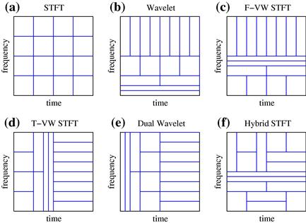
Figure 3.8 Time and frequency lattice illustration for: (a) the STFT with a constant window, (b) the wavelet transform, (c) a frequency-varying window (F-VW) STFT, (d) a time-varying window (T-VW) STFT, (e) the dual wavelet transform, and (f) a hybrid STFT with time and frequency varying window.
Frequency varying window
The STFT can be calculated by using the signal’s DFT instead of the signal. There is a direct relation between the time and the frequency domain STFT via coefficients of the form ![]() . A dual form of the STFT is:
. A dual form of the STFT is:
 (3.24)
![]()
Frequency domain window may be of frequency varying width (Figure 3.8). This form is dual to the time-varying form.
Hybrid time and frequency varying windows
In general, spectral content of signal changes in time and frequency in an arbitrary manner. There are several methods in the literature that adapt windows or basis functions to the signal form for each time instant or even for every considered time and frequency point in the time-frequency plane (e.g., as in Figure 3.8). Selection of the most appropriate form of the basis functions (windows) for each time-frequency point includes a criterion for selecting the optimal window width (basis function scale) for each point.
If we consider a signal with N samples, then its time-frequency plane can be split in a large number of different grids for the non-overlapping STFT calculation. All possible variations of time-varying or frequency-varying windows, are just special cases of general hybrid time-varying grid. Covering a time-frequency ![]() plane, by any combination of non-overlapping rectangular areas, whose individual area is N, corresponds to a valid non-overlapping STFT calculation scheme. The total number of ways
plane, by any combination of non-overlapping rectangular areas, whose individual area is N, corresponds to a valid non-overlapping STFT calculation scheme. The total number of ways ![]() , how an
, how an ![]() plane can be split (into non-overlapping STFTs of area N with dyadic time-varying windows) is:
plane can be split (into non-overlapping STFTs of area N with dyadic time-varying windows) is:
![]()
The approximative formula for ![]() can be written in the form, [6]:
can be written in the form, [6]:
![]() (3.25)
(3.25)
where ![]() stands for an integer part of the argument. It holds with relative error smaller than
stands for an integer part of the argument. It holds with relative error smaller than ![]() for
for ![]() . For example, for
. For example, for ![]() we have
we have ![]() different ways to split time-frequency plane into non-overlapping time-frequency regions with dyadic time-varying windows. Of course, most of them cannot be considered within the either time-varying or frequency-varying window case, since they are time-frequency varying (hybrid) in general.
different ways to split time-frequency plane into non-overlapping time-frequency regions with dyadic time-varying windows. Of course, most of them cannot be considered within the either time-varying or frequency-varying window case, since they are time-frequency varying (hybrid) in general.
3.03.2.2.3 Signal reconstruction form the discrete STFT
Signal reconstruction from non-overlapping STFT values is obvious, according to (3.20), (3.22), or (3.23).
Signal can be reconstructed from the STFT calculated with N signal samples, if the calculated STFT is overlapped, i.e., down-sampled in time by ![]() . Here, the signal general reconstruction scheme from the STFT values, overlapped in time, will be presented. Consider the STFT, (3.16), written in a vector form, as
. Here, the signal general reconstruction scheme from the STFT values, overlapped in time, will be presented. Consider the STFT, (3.16), written in a vector form, as
 (3.26)
where the vector ![]() contains all frequency values of the STFT, for a given n,
contains all frequency values of the STFT, for a given n,
![]()
Signal vector is
![]()
while ![]() is the DFT matrix with coefficients
is the DFT matrix with coefficients ![]() . A diagonal matrix
. A diagonal matrix ![]() is the window matrix
is the window matrix ![]() and
and ![]() for
for ![]() .
.
It has been assumed that the STFTs are calculated with a step ![]() in time. So they are overlapped for
in time. So they are overlapped for ![]() . Available STFT values are
. Available STFT values are
Based on the available STFT values (3.26), the windowed signal values can be reconstructed as
![]() (3.27)
(3.27)
For ![]() we get
we get
 (3.28)
Let us reindex the reconstructed signal value (3.28) by substitution ![]()
By summing over i satisfying ![]() we get that the reconstructed signal is undistorted (up to a constant) if
we get that the reconstructed signal is undistorted (up to a constant) if
![]() (3.29)
(3.29)
Special cases:
1. For ![]() (non-overlapping), relation (3.29) is satisfied for the rectangular window, only.
(non-overlapping), relation (3.29) is satisfied for the rectangular window, only.
2. For a half of the overlapping period, ![]() , condition (3.29) is met for the rectangular, Hann(ing), Hamming, triangular,…, windows.
, condition (3.29) is met for the rectangular, Hann(ing), Hamming, triangular,…, windows.
3. The same holds for ![]() , if the values of R are integers.
, if the values of R are integers.
4. For ![]() (the STFT calculation in each available time instant), any window satisfies the inversion relation.
(the STFT calculation in each available time instant), any window satisfies the inversion relation.
In analysis of non-stationary signals our primary interest is not in signal reconstruction with the fewest number of calculation points. Rather, we are interested in tracking signals’ non-stationary parameters, like for example, instantaneous frequency. These parameters may significantly vary between neighboring time instants n and ![]() . Quasi-stationarity of signal within R samples (implicitly assumed when down-sampling by factor of R is done) in this case is not a good starting point for the analysis. Here, we have to use the time-frequency analysis of signal at each instant n, without any down-sampling. Very efficient realizations, for this case, are the recursive ones.
. Quasi-stationarity of signal within R samples (implicitly assumed when down-sampling by factor of R is done) in this case is not a good starting point for the analysis. Here, we have to use the time-frequency analysis of signal at each instant n, without any down-sampling. Very efficient realizations, for this case, are the recursive ones.
3.03.2.3 Gabor transform
The Gabor transform is the oldest time-frequency form applied in the signal processing field (since the Wigner distribution remained for a long time within the quantum mechanics, only). It has been introduced with the aim to expand a signal ![]() into a series of time-frequency shifted elementary functions
into a series of time-frequency shifted elementary functions ![]() (logons)
(logons)
![]() (3.30)
(3.30)
The Gabor’s original choice was the Gaussian window

due to its best concentration in the time-frequency plane. Gabor also used ![]() .
.
In the time frequency-domain, the elementary functions ![]() are shifted in time and frequency for nT and
are shifted in time and frequency for nT and ![]() , respectively.
, respectively.
For the analysis of signal, Gabor has divided the whole information (time-frequency) plane by a grid at ![]() and
and ![]() , with area of elementary cell
, with area of elementary cell ![]() . Then, the signal is expanded at the central points of the grid
. Then, the signal is expanded at the central points of the grid ![]() using the elementary atom functions
using the elementary atom functions ![]()
![]() .
.
If the elementary functions ![]() were orthogonal to each other, i.e.,
were orthogonal to each other, i.e.,
![]()
then by multiplying (3.30) by ![]() and integrating over t we could get
and integrating over t we could get
![]()
which corresponds to the STFT at ![]() . However, the elementary logons do not satisfy the orthogonality property. Gabor originally proposed an iterative procedure for the calculation of
. However, the elementary logons do not satisfy the orthogonality property. Gabor originally proposed an iterative procedure for the calculation of ![]() .
.
Interest in the Gabor transform, had been lost for decades, until a simplified procedure for the calculation of coefficients has been developed. This procedure is based on introducing elementary signal ![]() dual to
dual to ![]() such that
such that
![]()
holds (Bastiaans logons). Then
![]()
However, the dual function ![]() has a poor time-frequency localization. In addition, there is no stable algorithm to reconstruct the signal with the critical sampling condition
has a poor time-frequency localization. In addition, there is no stable algorithm to reconstruct the signal with the critical sampling condition ![]() . One solution is to use an oversampled set of functions with
. One solution is to use an oversampled set of functions with ![]() .
.
3.03.2.4 Stationary phase method
When the signal
![]()
is not of simple analytic form, it may be possible, in some cases, to obtain an approximative expression for the FT by using the method of stationary phase [24,25].
The method of stationary phase states:
If the function ![]() is monotonous and
is monotonous and ![]() is sufficiently smooth function, then
is sufficiently smooth function, then
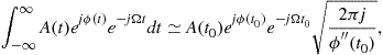 (3.31)
where ![]() is the solution of
is the solution of
![]()
The most significant contribution to the integral on the left side of (3.31) comes from the region where the phase of the exponential function ![]() is stationary in time, since the contribution of the intervals with fast varying
is stationary in time, since the contribution of the intervals with fast varying ![]() tends to zero. In other words, in the considered time region, the signal’s phase
tends to zero. In other words, in the considered time region, the signal’s phase ![]() behaves as
behaves as ![]() . Thus, we may say that the rate of the phase change,
. Thus, we may say that the rate of the phase change, ![]() , for that particular instant is its instantaneous frequency corresponding to frequency
, for that particular instant is its instantaneous frequency corresponding to frequency ![]() . The stationary point
. The stationary point ![]() of phase
of phase ![]() , of signal
, of signal ![]() , is obtained as a solution of
, is obtained as a solution of
![]()
By expanding ![]() into a Taylor series up to the second order term, around the stationary point
into a Taylor series up to the second order term, around the stationary point ![]() , we have
, we have
 (3.32)
Using the FT pair
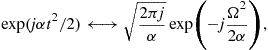
for a large ![]() it follows
it follows ![]() , i.e.,
, i.e.,
![]() (3.33)
(3.33)
Relation (3.31) is now easily obtained from (3.32) with (3.33), for large ![]() .
.
If the equation ![]() has two (or more) solutions
has two (or more) solutions ![]() and
and ![]() then the integral on the left side of (3.31) is equal to the sum of functions at both (or more) stationary phase points. Finally, this relation holds for
then the integral on the left side of (3.31) is equal to the sum of functions at both (or more) stationary phase points. Finally, this relation holds for ![]() . If
. If ![]() then similar analysis may be performed, using the lowest non-zero phase derivative at the stationary phase point.
then similar analysis may be performed, using the lowest non-zero phase derivative at the stationary phase point.
Example 2
Consider a frequency modulated signal
![]()
By using the stationary phase method we get that the stationary phase point is ![]() with
with ![]() and
and ![]() . The amplitude and phase of
. The amplitude and phase of ![]() , according to (3.31), are
, according to (3.31), are

for a large value of a. The integrand in (3.31) is illustrated in Figure 3.9, for ![]() , when
, when ![]() and
and ![]() .
.

3.03.2.4.1 Instantaneous frequency
Here, we present a simple instantaneous frequency (IF) interpretation when signal may be considered as stationary within the localization window (quasistationary signal). Consider a signal ![]() , within the window
, within the window ![]() of the width
of the width ![]() . If we can assume that the amplitude variations are small and the phase variations are almost linear within
. If we can assume that the amplitude variations are small and the phase variations are almost linear within ![]() , i.e.,
, i.e.,
![]()
![]()
Thus, around a given instant t, the signal behaves as a sinusoid in the ![]() domain with amplitude
domain with amplitude ![]() , phase
, phase ![]() , and frequency
, and frequency ![]() . The first derivative of phase,
. The first derivative of phase, ![]() , plays the role of frequency within the considered lag interval around t.
, plays the role of frequency within the considered lag interval around t.
The stationary phase method relates the spectral content at the frequency ![]() with the signal’s value at time instant t, such that
with the signal’s value at time instant t, such that ![]() . A signal in time domain, that satisfies stationary phase method conditions, contributes at the considered instant t to the FT at the corresponding frequency
. A signal in time domain, that satisfies stationary phase method conditions, contributes at the considered instant t to the FT at the corresponding frequency
![]()
Additional comments on this relation are given within the stationary phase method presentation subsection.
The instantaneous frequency is not so clearly defined as the frequency in the FT. For example, the frequency in the FT has the physical interpretation as the number of signal periods within the considered time interval, while this interpretation is not possible if a single time instant is considered. Thus, a significant caution has to be taken in using this notion. Various definitions and interpretations of the IF are given in the literature, with the most comprehensive review presented by Boashash.
Example 3
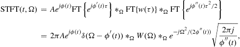
The STFT of the signal
![]()
can be approximately calculated for a large a, by using the method of stationary phase, as
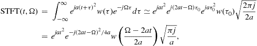
where the stationary point ![]() is obtained from
is obtained from
![]()
Note that the absolute value of the STFT reduces to
![]() (3.34)
(3.34)
In this case, the width of ![]() in frequency does not decrease with the increase of the window
in frequency does not decrease with the increase of the window ![]() width. The width of
width. The width of ![]() around the central frequency
around the central frequency ![]() is
is
![]()
where ![]() is the window width in time domain. Note that this relation holds for a wide window
is the window width in time domain. Note that this relation holds for a wide window ![]() such that the stationary phase method may be applied. If the window is narrow with respect to the phase variations of the signal, the STFT width is defined by the width of the FT of window, being proportional to
such that the stationary phase method may be applied. If the window is narrow with respect to the phase variations of the signal, the STFT width is defined by the width of the FT of window, being proportional to ![]() . Thus, the overall STFT width is equal to the sum of the frequency variation caused width and the window’s FT width, i.e.,
. Thus, the overall STFT width is equal to the sum of the frequency variation caused width and the window’s FT width, i.e.,
![]()
where c is a constant defined by the window shape. Therefore, there is a window width T producing the narrowest possible STFT for this signal. It is obtained by equating the derivative of the overall width to zero, ![]() , which results in
, which results in
![]()
As expected, for a sinusoid, ![]() .
.
Consider now the general form of FM signal
![]()
where ![]() is a differentiable function. Its STFT is of the form
is a differentiable function. Its STFT is of the form
where ![]() is expanded into the Taylor series around t as
is expanded into the Taylor series around t as
![]()
Neglecting the higher order terms in the Taylor series we can write
where ![]() denotes the convolution in frequency. As expected, the influence of the window is manifested as a spread of ideal concentration
denotes the convolution in frequency. As expected, the influence of the window is manifested as a spread of ideal concentration ![]() . In addition, the term due to the frequency non-stationarity
. In addition, the term due to the frequency non-stationarity ![]() causes an additional spread. This relation confirms our previous conclusion that the overall STFT width is the sum of the width of
causes an additional spread. This relation confirms our previous conclusion that the overall STFT width is the sum of the width of ![]() and the width caused by the signal’s non-stationarity.
and the width caused by the signal’s non-stationarity.
3.03.2.5 Local polynomial Fourier transform
There are signals whose form is known up to an unknown set of parameters. For example, many signals could be expressed as polynomial-phase signal
![]()
with (unknown) parameters ![]() High concentration of such signals in the frequency domain is achieved by the polynomial FT defined by
High concentration of such signals in the frequency domain is achieved by the polynomial FT defined by
![]()
when parameters ![]() are equal to the signal parameters
are equal to the signal parameters ![]() Finding values of unknown parameters
Finding values of unknown parameters ![]() that match signal parameters can be done by a simple search over a possible set of values for
that match signal parameters can be done by a simple search over a possible set of values for ![]() and stopping the search when the maximally concentrated distribution is achieved (in ideal case, the delta function at
and stopping the search when the maximally concentrated distribution is achieved (in ideal case, the delta function at ![]() , for
, for ![]() is obtained). This procedure may be time consuming.
is obtained). This procedure may be time consuming.
For non-stationary signals, this approach may be used if the non-stationary signal could be considered as a signal with constant parameters within the analysis window. In that case, the local polynomial Fourier transform (LPFT), proposed by Katkovnik, may be used [26]. It is defined as
![]()
Example 4
Consider the second order polynomial-phase signal
![]()
Its LPFT has the form
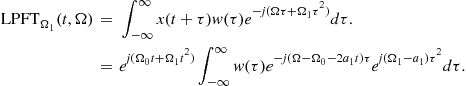
For ![]() , the second-order phase term does not introduce any distortion to the local polynomial spectrogram,
, the second-order phase term does not introduce any distortion to the local polynomial spectrogram,
![]()
with respect to the spectrogram of a sinusoid with constant frequency. For a wide window ![]() , like in the case of the STFT of a pure sinusoid, we achieve high concentration.
, like in the case of the STFT of a pure sinusoid, we achieve high concentration.
The LPFT could be considered as the FT of signal demodulated with ![]() . Thus, if we are interested in signal filtering, we can find the coefficients
. Thus, if we are interested in signal filtering, we can find the coefficients ![]() , demodulate the signal by multiplying it with
, demodulate the signal by multiplying it with ![]() and use a standard filter for a pure sinusoid.
and use a standard filter for a pure sinusoid.
In general, we can extend this approach to any signal ![]() by estimating its phase
by estimating its phase ![]() with
with ![]() (using the instantaneous frequency estimation that will be discussed later) and filtering demodulated signal
(using the instantaneous frequency estimation that will be discussed later) and filtering demodulated signal ![]() by a low-pass filter. The resulting signal is obtained when the filtered signal is returned back to the original frequencies, by modulation with
by a low-pass filter. The resulting signal is obtained when the filtered signal is returned back to the original frequencies, by modulation with ![]() .
.
The filtering of signal can be modeled by the following expression:
![]() (3.35)
(3.35)
where ![]() is the LPFT of
is the LPFT of ![]() is the filtered signal,
is the filtered signal, ![]() is a support function used for filtering. It could be 1 within the time-frequency region where we assume that the signal of interest exists, and 0 elsewhere.
is a support function used for filtering. It could be 1 within the time-frequency region where we assume that the signal of interest exists, and 0 elsewhere.
Note that the sufficient order of the LPFT can be obtained recursively. We start from the STFT and check whether its auto-term’s width is equal to the width of the FT of the used window. If true, it means that a signal is a pure sinusoid and the STFT provides its best possible concentration. We should not calculate the LPFT. If the auto-term is wider, it means that there are signal non-stationarities within the window and the first-order LPFT should be calculated. The auto-term’s width is again compared to the width of the window’s FT and if they do not coincide we should increase the LPFT order.
In case of multi-component signals, the distribution will be optimized to the strongest component first. Then, the strongest component is filtered out and the procedure is repeated for the next component in the same manner, until the energy of the remaining signal is negligible, i.e., until all the components are processed.
3.03.2.6 Relation between the STFT and the continuous wavelet transform
The first form of functions having the basic property of wavelets was used by Haar at the beginning of the 20th century. At the beginning of 1980s, Morlet introduced a form of basis functions for analysis of seismic signals, naming them “wavelets.” Theory of wavelets was linked to the image processing by Mallat in the following years. In late 1980s Daubechies presented a whole new class of wavelets that, in addition to the orthogonality property, can be implemented in a simple way, by using digital filtering ideas. The most important applications of the wavelets are found in image processing and compression, pattern recognition and signal denoising. As such they will be a separate topic of this book. Here, we will only link continuous wavelet transform to the time-frequency analysis [5,27,28].
The STFT is characterized by constant time and frequency resolutions for both low and high frequencies. The basic idea behind the wavelet transform is to vary the resolutions with scale (being related to frequency), so that a high frequency resolution is obtained for low frequencies, whereas a high time resolution is obtained for high frequencies, which could be relevant for some practical applications. It is achieved by introducing a variable window width, such that it is decreased for higher frequencies. The basic idea of the wavelet transform and its comparison with the STFT is illustrated in Figure 3.10.

Figure 3.10 Expansion functions for the wavelet transform (left) and the short-time Fourier transform (right). Top row presents high scale (low frequency), middle row is for a medium scale (medium frequency) and bottom row is for a low scale (high frequency).
Time and frequency resolution is schematically illustrated in Figure 3.8.
When the above idea is translated into the mathematical form, one gets the definition of a continuous wavelet transform
![]() (3.36)
(3.36)
where ![]() is a band-pass signal, and the parameter a is the scale. This transform produces a time-scale, rather than the time-frequency signal representation. For the Morlet wavelet (that will be used for illustrations in this short presentation) the relation between the scale and the frequency is
is a band-pass signal, and the parameter a is the scale. This transform produces a time-scale, rather than the time-frequency signal representation. For the Morlet wavelet (that will be used for illustrations in this short presentation) the relation between the scale and the frequency is ![]() . In order to establish a strong formal relationship between the WT and the STFT, we will choose the basic wavelet
. In order to establish a strong formal relationship between the WT and the STFT, we will choose the basic wavelet ![]() in the form
in the form
![]() (3.37)
(3.37)
where ![]() is a window function and
is a window function and ![]() is a constant frequency. For example, for the Morlet wavelet we have a modulated Gaussian function
is a constant frequency. For example, for the Morlet wavelet we have a modulated Gaussian function
![]()
where the values of ![]() and
and ![]() are chosen such that the ratio of
are chosen such that the ratio of ![]() and the first maximum is
and the first maximum is ![]() . From the definition of
. From the definition of ![]() it is obvious that small
it is obvious that small ![]() (i.e., large a) corresponds to a wide wavelet, i.e., a wide window, and vice versa.
(i.e., large a) corresponds to a wide wavelet, i.e., a wide window, and vice versa.
Substitution of (3.37) into (3.36) leads to a continuous wavelet transform form suitable for a direct comparison with the STFT:
![]() (3.38)
(3.38)
From the filter theory point of view the wavelet transform, for a given scale a, could be considered as the output of system with impulse response ![]() , i.e.,
, i.e., ![]() , where
, where ![]() denotes a convolution in time. Similarly the STFT, for a given
denotes a convolution in time. Similarly the STFT, for a given ![]() , may be considered as
, may be considered as ![]() . If we consider these two band-pass filters from the bandwidth point of view we can see that, in the case of STFT, the filtering is done by a system whose impulse response
. If we consider these two band-pass filters from the bandwidth point of view we can see that, in the case of STFT, the filtering is done by a system whose impulse response ![]() has a constant bandwidth, being equal to the width of the FT of
has a constant bandwidth, being equal to the width of the FT of ![]() .
.
The S-transform (or the Stockwell transform) is conceptually a hybrid of short-time Fourier analysis and wavelet analysis. It employs a variable window length but preserves the phase information by using the STFT form in the signal decomposition. As a result, the phase spectrum is absolute in the sense that it is always referred to a fixed time reference. The real and imaginary spectrum can be localized independently with resolution in time in terms of basis functions. The changes in the absolute phase of a certain frequency can be tracked along the time axis and useful information can be extracted. In contrast to wavelet transform, the phase information provided by the S-transform is referenced to the time origin, and therefore provides supplementary information about spectra which is not available from locally referenced phase information obtained by the continuous wavelet transform. The frequency dependent window function produces higher frequency resolution at lower frequencies, while at higher frequencies sharper time localization can be achieved.Constant Q-factor transformThe quality factor Q for a band-pass filter, as measure of the filter selectivity, is defined as
![]()
In the STFT the bandwidth is constant, equal to the window FT width, ![]() . Thus, factor Q is proportional to the considered frequency,
. Thus, factor Q is proportional to the considered frequency,
![]()
In the case of the wavelet transform the bandwidth of impulse response is the width of the FT of ![]() . It is equal to
. It is equal to ![]() , where
, where ![]() is the constant bandwidth corresponding to the mother wavelet. It follows
is the constant bandwidth corresponding to the mother wavelet. It follows
![]()
Therefore, the continuous wavelet transform corresponds to the passing a signal through a series of band-pass filters centered at ![]() , with constant factor Q. Again we can conclude that the filtering, that produces WT, results in a small bandwidth (high frequency resolution and low time resolution) at low frequencies and wide bandwidth (low frequency and high time resolution) at high frequencies.
, with constant factor Q. Again we can conclude that the filtering, that produces WT, results in a small bandwidth (high frequency resolution and low time resolution) at low frequencies and wide bandwidth (low frequency and high time resolution) at high frequencies.
Affine transforms
A whole class of signal representations, including the quadratic ones, is defined with the aim to preserve the constant Q property. They belong to the area of the so called time-scale signal analysis or affine time-frequency representations [5,14,28–31]. The basic property of an affine time-frequency representation is that the representation of time shifted and scaled version of signal
![]()
whose FT is ![]() , results in a time-frequency representation
, results in a time-frequency representation
![]()
The name affine comes from the affine transformation of time, that is, in general a transformation of the form ![]() . It is easy to verify that continuous wavelet transform satisfies this property.
. It is easy to verify that continuous wavelet transform satisfies this property.
Example 5
Consider signal (3.6). Its continuous wavelet transform is
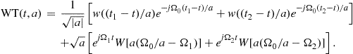 (3.39)
The transform (3.39) has non-zero values in the region depicted in Figure 3.11a.

Scalogram:
In analogy with spectrogram, the scalogram is defined as the squared magnitude of a wavelet transform:
![]() (3.40)
(3.40)
The scalogram obviously loses the linearity property, and fits into the category of quadratic transforms.
A Simple filter bank formulation
Time-frequency grid for wavelet transform is presented in Figure 3.8. Within the filter bank framework in means that the original signal is processed in the following way. The signal’s spectral content is divided into high frequency and low frequency part. An example, how to achieve this is presented in the STFT analysis by using a two samples rectangular window ![]() , with
, with ![]() . Then, its two samples WT is
. Then, its two samples WT is ![]() , for
, for ![]() , corresponding to low frequency
, corresponding to low frequency ![]() and
and ![]() for
for ![]() corresponding to high frequency
corresponding to high frequency ![]() . The high frequency part,
. The high frequency part, ![]() , having high resolution in time, is not processed any more. It is kept with this high resolution in time, expecting that this kind of resolution will be needed for a signal. The low pass part
, having high resolution in time, is not processed any more. It is kept with this high resolution in time, expecting that this kind of resolution will be needed for a signal. The low pass part ![]() is further processed, by dividing it into its low frequency part,
is further processed, by dividing it into its low frequency part,
![]()
![]()
The high pass of this part is left with resolution four in time, while the low pass part is further processed, by dividing it into its low and high frequency part, until the full length of signal is achieved, Figure 3.8b.
Chirplet transform
An extension of the wavelet transform, for time-frequency analysis, is the chirplet transform. By using linear frequency modulated forms instead of the constant frequency ones, the chirplet is formed. Here we will present a Gaussian chirplet atom that is a four parameter function

where the parameter ![]() controls the width of the chirplet in time, parameter
controls the width of the chirplet in time, parameter ![]() stands for the chirplet rate in time-frequency plane, while t and
stands for the chirplet rate in time-frequency plane, while t and ![]() are the coordinates of the central time and frequency point in the time-frequency plane. In this way, for a given parameters
are the coordinates of the central time and frequency point in the time-frequency plane. In this way, for a given parameters ![]() we project signal onto a Gaussian chirp, centered at
we project signal onto a Gaussian chirp, centered at ![]() whose width is defined by
whose width is defined by ![]() and rate is
and rate is ![]() :
:
![]()
In general, projection procedure should be performed for each point in time-frequency plane, for all possible parameter values. Interest in using a Gaussian chirplet atom stems from to the fact that it provides the highest joint time-frequency concentration. In practice, all four parameters should be discretized. The set of the parameter discretized atoms are called a dictionary. In contrast to the second order local polynomial FT, here the window width is parametrized and varies, as well. Since we have a multiparameter problem, computational requirements for this transform are very high.
In order to improve efficiency of the chirplet transform calculation, various adaptive forms of the chirplet transform were proposed. The matching pursuit procedure is a typical example. The first step of this procedure is to choose a chirplet atom from the dictionary yielding the largest amplitude of the inner product between the atom and the signal. Then the residual signal, obtained after extracting the first atom, is decomposed in the same way. Consequently, the signal is decomposed into a sum of chirplet atoms.
3.03.2.7 Generalization
In general, any set of well localized functions in time and frequency can be used for the time-frequency analysis of a signal. Let us denote signal as ![]() and the set of such functions with
and the set of such functions with ![]() , then the projection of the signal
, then the projection of the signal ![]() onto such functions,
onto such functions,
![]()
represents similarity between ![]() and
and ![]() , at a given point with parameter values defined by
, at a given point with parameter values defined by ![]() .
.
We may have the following cases:
• Frequency as the only one parameter. Then, we have projection onto complex harmonics with changing frequency, and ![]() is the FT of signal
is the FT of signal ![]() with
with
![]()
• Time and frequency as parameters. Varying t and ![]() and calculating projections of signal
and calculating projections of signal ![]() we get the STFT. In this case we use
we get the STFT. In this case we use ![]() as a localization function around parameter t and
as a localization function around parameter t and
![]()
• Time and frequency as parameters with a frequency dependent localization in time, we get wavelet transform. It is more often expressed as function of scale parameter ![]() , than the frequency
, than the frequency ![]() . The S-transform belongs to this class. For the continuous wavelet transform with mother wavelet
. The S-transform belongs to this class. For the continuous wavelet transform with mother wavelet ![]() we have
we have
![]()
• Frequency and signal phase rate. We get the polynomial FT of the second order, with
![]()
• Time, frequency, and signal phase rate as parameters results in a form of the local polynomial Fourier transform with
![]()
• Time, frequency, and signal phase rate as parameters, with a varying time localization, as parameters results in the chirplets with localization function with
![]()
• Frequency, signal phase rate, and other higher order coefficients, we get the polynomial FT of the Nth order, with
![]()
• Time, frequency, signal phase rate, and other higher order coefficients, we get the local polynomial FT of the Nth order, with
![]()
• Time, frequency, signal phase rate, and other higher order coefficients, with a variable window width we would get the Nth order-lets, with
![]()
• Time, frequency, and any other parametrized phase function form, like sinusoidal ones, with constant or variable window width![]()
3.03.3 Quadratic time-frequency distributions
In order to provide additional insight into the field of joint time-frequency analysis, as well as to improve concentration of time-frequency representation, energy distributions of signals were introduced. We have already mentioned the spectrogram which belongs to this class of representations and is a straightforward extension of the STFT. Here, we will discuss other distributions and their generalizations.
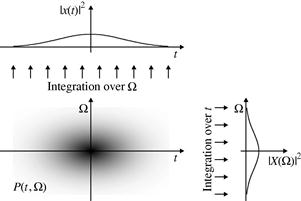
The basics condition for the definition of time-frequency energy distributions is that a two-dimensional function of time and frequency ![]() represents the energy density of a signal in the time-frequency plane. Thus, the signal energy associated with the small time and frequency intervals
represents the energy density of a signal in the time-frequency plane. Thus, the signal energy associated with the small time and frequency intervals ![]() and
and ![]() , respectively, would be
, respectively, would be
![]()
However, point by point definition of time-frequency energy densities in the time-frequency plane is not possible, since the uncertainty principle prevents us from defining concept of energy at a specific instant and frequency. This is the reason why some more general conditions are being considered to derive time-frequency distributions of a signal. Namely, one requires that the integral of ![]() over
over ![]() , for a particular instant of time should be equal to the instantaneous power of the signal
, for a particular instant of time should be equal to the instantaneous power of the signal ![]() , while the integral over time for a particular frequency should be equal to the spectral energy density
, while the integral over time for a particular frequency should be equal to the spectral energy density ![]() . These conditions are known as marginal conditions or marginal properties of time-frequency distributions.
. These conditions are known as marginal conditions or marginal properties of time-frequency distributions.
Therefore, it is desirable that an energetic time-frequency distribution of a signal ![]() satisfies:
satisfies:
where ![]() denotes the energy of
denotes the energy of ![]() . It is obvious that if either one of marginal properties (3.42), (3.43) is fulfilled, so is the energy property. Note that relations (3.41)–(3.43), do not reveal any information about the local distribution of energy at a point
. It is obvious that if either one of marginal properties (3.42), (3.43) is fulfilled, so is the energy property. Note that relations (3.41)–(3.43), do not reveal any information about the local distribution of energy at a point ![]() . The marginal properties are illustrated in Figure 3.12.
. The marginal properties are illustrated in Figure 3.12.
Next we will introduce some distributions satisfying these properties.
3.03.3.1 Rihaczek distribution
The Rihaczek distribution satisfies the marginal properties (3.41)–(3.43). This distribution is of limited practical importance (some recent contributions show that it could be interesting in the phase synchrony and stochastic signal analysis). We will present one of its derivations with a simple electrical engineering foundation.
Consider a simple electrical circuit analysis. Assume that a voltage ![]() is applied at the resistor whose resistance is
is applied at the resistor whose resistance is ![]() , but only within a very narrow frequency band
, but only within a very narrow frequency band ![]()

In that case, the energy dissipated at the resistor within a short time interval ![]() is defined as:
is defined as:
![]() (3.44)
(3.44)
where ![]() denotes the resulting current. It may be expressed in terms of the FT of the voltage:
denotes the resulting current. It may be expressed in terms of the FT of the voltage:
![]() (3.45)
(3.45)
where capital letters represent corresponding FTs of the current and voltage. Substitution of (3.45) into (3.44) produces
![]() (3.46)
(3.46)
Based on the above considerations, one may define a time-frequency energy distribution:
![]() (3.47)
(3.47)
The previous analysis may be generalized for an arbitrary signal ![]() with the associated FT
with the associated FT ![]() . The Rihaczek distribution is obtained in the following form:
. The Rihaczek distribution is obtained in the following form:
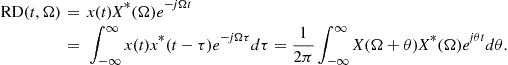 (3.48)
It seems that the Rihaczek distribution is an ideal one, we have been looking for. However, energy is calculated over the intervals ![]() and
and ![]() , while
, while ![]() was calculated over the entire interval
was calculated over the entire interval ![]() . This introduces the influence of other time periods onto the interval
. This introduces the influence of other time periods onto the interval ![]() . Therefore, it is not as local as it may seem from the derivation. This distribution exhibits significant drawbacks for possible time-frequency analysis, as well. The most important one is that it is complex valued, despite the fact that it has been derived with the aim to represent signal energy density. In addition, its time-frequency concentration for non-stationary signals is quite low.
. Therefore, it is not as local as it may seem from the derivation. This distribution exhibits significant drawbacks for possible time-frequency analysis, as well. The most important one is that it is complex valued, despite the fact that it has been derived with the aim to represent signal energy density. In addition, its time-frequency concentration for non-stationary signals is quite low.
3.03.3.2 Wigner distribution
The other quadratic distributions cannot be easily derived as the Rihaczek distribution. Partially this is due to the lack of adequate simple physical interpretations. In order to derive some other quadratic time-frequency distributions, observe that the Rihaczek distribution may be interpreted as the FT (over ![]() ) of the function
) of the function
![]()
that will be referred to as the local autocorrelation function,
![]() (3.49)
(3.49)
This relation is in accordance with spectral density function for random signals. A general form of the local autocorrelation function may be written as
![]() (3.50)
(3.50)
where ![]() is an arbitrary constant (
is an arbitrary constant (![]() produces the RD; note that also
produces the RD; note that also ![]() could be used as a variant of the RD). For
could be used as a variant of the RD). For ![]() , the local autocorrelation function
, the local autocorrelation function ![]() is Hermitian, i.e.,
is Hermitian, i.e.,
![]() (3.51)
(3.51)
and its FT is real valued. The distribution that satisfies this property is called the Wigner distribution (or the Wigner-Ville distribution). It is defined as
![]() (3.52)
(3.52)
The Wigner distribution is originally introduced in quantum mechanics.
Expressing ![]() in terms of
in terms of ![]() and substituting it into (3.52) we get
and substituting it into (3.52) we get
![]() (3.53)
(3.53)
what represents a definition of the Wigner distribution in the frequency domain.
A distribution defined as the FT of (3.50) is called the Generalized Wigner Distribution (GWD). The name stems from the fact that this distribution is based on the Wigner distribution (for ![]() ), which is the most important member of this class of distributions.
), which is the most important member of this class of distributions.
It is easy to show that the Wigner distribution and all the other distributions from the GWD class satisfy the marginal properties. From the Wigner distribution definition, it follows
![]() (3.54)
(3.54)
which, for ![]() , produces (3.42)
, produces (3.42)
![]() (3.55)
(3.55)
Based on the definition of the Wigner distribution in the frequency domain, (3.53), one may easily prove the fulfillment of the frequency marginal. The marginal properties are satisfied for the whole class of GWD.
Example 6
The Wigner distribution of signals ![]() and
and ![]() is given by
is given by
![]()
and
![]()
respectively. The distribution concentration is very high, in both cases. Note that this fact does not mean that, for one signal component, we will be able to achieve an arbitrary high concentration simultaneously in both time and in frequency.
Example 7
Let us now assume a linear frequency modulated signal, ![]() . In this case we have
. In this case we have
![]()
with
![]()
Again, a high concentration in the time-frequency plane is achieved.
These two examples demonstrated that the Wigner distribution can provide superior time-frequency representations in comparison to the STFT.
3.03.3.2.1 Distribution concentrated at the instantaneous frequency
For a general mono-component signal of the form ![]() , with slow varying amplitude comparing to the signal phase variations
, with slow varying amplitude comparing to the signal phase variations ![]() , an ideal time-frequency (ITF) representation (fully concentrated along the instantaneous frequency) can be defined as:
, an ideal time-frequency (ITF) representation (fully concentrated along the instantaneous frequency) can be defined as:
![]() (3.56)
(3.56)
Note that the ideal TFD defined by (3.56) satisfies the marginal properties for a wide class of frequency modulated signals. The time marginal is satisfied since:
![]()
where a monotonous function ![]() is assumed, with
is assumed, with ![]() being the solution of
being the solution of ![]() . Since the time marginal condition is satisfied, so is the energy condition. For signals satisfying the stationary phase method, the frequency marginal is satisfied, as well. From a similar analysis in the frequency domain one may define a distribution fully concentrated along the group delay, as well.
. Since the time marginal condition is satisfied, so is the energy condition. For signals satisfying the stationary phase method, the frequency marginal is satisfied, as well. From a similar analysis in the frequency domain one may define a distribution fully concentrated along the group delay, as well.
For a frequency modulated signal ![]() the Wigner distribution (3.52) assumes the form:
the Wigner distribution (3.52) assumes the form:
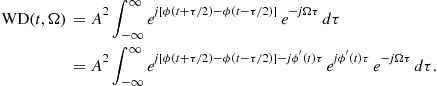
Factor ![]() produces the ideal distribution concentration
produces the ideal distribution concentration ![]() , while the term
, while the term
![]() (3.57)
(3.57)
causes distribution spread around the instantaneous frequency. Factor Q will be refereed to as the spread factor. It is equal to zero if instantaneous frequency ![]() is a linear function, i.e., if
is a linear function, i.e., if ![]() , for
, for ![]() .
.
Example 8
Let us consider signal of the form
![]()
The Wigner distribution of ![]() is FT of
is FT of

Note that the duration in time is proportional to ![]() while the duration in frequency is proportional to
while the duration in frequency is proportional to ![]() . Product of these durations is constant.
. Product of these durations is constant.
3.03.3.2.2 Signal reconstruction
The signal can be reconstructed from the Wigner distribution, Eq. (3.54) with ![]() , as:
, as:
![]()
Due to the term ![]() ambiguity in the signal phase remains.
ambiguity in the signal phase remains.
Since the Wigner distribution is a two-dimensional representation of a one-dimensional signal, obviously an arbitrary real valued two-dimensional function will not be a valid Wigner distribution. A two-dimensional real function ![]() is the Wigner distribution of a signal if:
is the Wigner distribution of a signal if:
![]() (3.58)
(3.58)
![]()
The solution of partial differential equation (3.58) is equal to ![]() , where
, where ![]() and
and ![]() are arbitrary functions of
are arbitrary functions of ![]() and
and ![]() . Therefore,
. Therefore, ![]() .
.
With ![]() and
and ![]() , we get:
, we get:
![]()
Since ![]() is a real function, it follows that
is a real function, it follows that ![]() . Thus, for
. Thus, for ![]() satisfying (3.58), there exists function
satisfying (3.58), there exists function ![]() such that
such that ![]() and
and ![]() are the FT pair. A mean squared approximation of an arbitrary two-dimensional function by a valid Wigner distribution, or a sum of the Wigner distributions, will be discussed later.
are the FT pair. A mean squared approximation of an arbitrary two-dimensional function by a valid Wigner distribution, or a sum of the Wigner distributions, will be discussed later.
3.03.3.2.3 Uncertainty principle and the Wigner distribution
The uncertainty principle for the Wigner distribution states that the product of effective durations of a signal ![]() in time
in time ![]() and in frequency
and in frequency ![]() cannot be arbitrary small. It satisfies the inequality:
cannot be arbitrary small. It satisfies the inequality:
![]() (3.59)
(3.59)
where ![]() and
and ![]() are defined by
are defined by
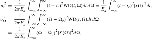 (3.60)
where ![]() is signal energy and
is signal energy and

The equality in (3.59) holds for the Gaussian signal ![]() , when we get
, when we get ![]() . Thus, it is not possible to achieve arbitrary high resolution in both directions, simultaneously. The product of effective durations is higher than
. Thus, it is not possible to achieve arbitrary high resolution in both directions, simultaneously. The product of effective durations is higher than ![]() for any other than the Gaussian signal.
for any other than the Gaussian signal.
The fact that the signal ![]() is located within
is located within ![]() in time and within
in time and within ![]() in frequency does not provide any information about the local concentration of the signal within this time-frequency region. It can be spread all over the region or highly concentrated along a line within that region. Thus, the conclusion that the Wigner distribution is highly concentrated along a line (that we made earlier for a linear FM signal), does not contradict the uncertainty principle. Local concentration measures are used to grade signal’s concentration in the time-frequency domain.
in frequency does not provide any information about the local concentration of the signal within this time-frequency region. It can be spread all over the region or highly concentrated along a line within that region. Thus, the conclusion that the Wigner distribution is highly concentrated along a line (that we made earlier for a linear FM signal), does not contradict the uncertainty principle. Local concentration measures are used to grade signal’s concentration in the time-frequency domain.
The duration of signal ![]() in frequency domain is
in frequency domain is
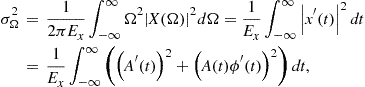
where, without loss of generality, ![]() is assumed. Note that the product
is assumed. Note that the product ![]() has a lower limit
has a lower limit ![]() , but there is no upper limit. It can be very large. Signals whose product of durations in time and frequency is large,
, but there is no upper limit. It can be very large. Signals whose product of durations in time and frequency is large, ![]() , are called asymptotic signals.
, are called asymptotic signals.
3.03.3.2.4 Pseudo quantum signal representation
A distribution that parametrize the uncertainty, keeping the marginal properties and the location of the instantaneous frequency, is defined as a “pseudo quantum” signal representation:
![]() (3.61)
(3.61)
with
![]()
The spreading factor in this representation is
![]()
For the Gaussian chirp signal
![]() (3.62)
(3.62)
we get
![]()
For a large parameter L, when ![]() , we get
, we get
![]()
being highly concentrated, simultaneously in time and in frequency ![]() at
at ![]() for a large a, if
for a large a, if ![]() . The uncertainty principle for (3.61) is
. The uncertainty principle for (3.61) is
![]() (3.63)
(3.63)
Note that the distribution ![]() satisfies the energy and the time marginal property for any set of parameters.
satisfies the energy and the time marginal property for any set of parameters.
The pseudo quantum signal representation of signal (3.62) with ![]() , and
, and ![]() for
for ![]() (Wigner distribution),
(Wigner distribution), ![]() and
and ![]() is given in Figure 3.13. The pseudo quantum distribution may be illustrated trough a physical experiment with a pendulum, for example, by changing the total acceleration of the pendulum system, as described in [6].
is given in Figure 3.13. The pseudo quantum distribution may be illustrated trough a physical experiment with a pendulum, for example, by changing the total acceleration of the pendulum system, as described in [6].
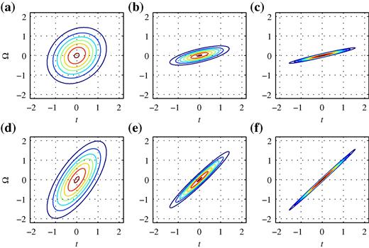
3.03.3.2.5 Instantaneous bandwidth
From the definition of the signal width in frequency (3.60) we can conclude that, at a given instant t, we may define similar local values
![]() (3.64)
(3.64)
with
![]()
playing a role of the instantaneous bandwidth ![]() and the mean frequency
and the mean frequency ![]() . It is easy to show that, for a signal
. It is easy to show that, for a signal ![]() , the mean frequency is equal to the instantaneous frequency,
, the mean frequency is equal to the instantaneous frequency,
![]()
This relation is used for the instantaneous frequency estimation, in addition to the simple detection of maximum position, for a given t.
For the instantaneous bandwidth we easily get:
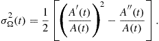
Note that both of these forms follow as special cases of conditional instantaneous moments. The nth conditional moment of the Wigner distribution, at an instant t, is defined as
![]()
Using the fact that the Wigner distribution and the local autocorrelation function are the FT pair, ![]() , resulting in
, resulting in
![]()
the moments are calculated as
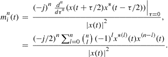
In a similar way we can define moments for other distributions from the generalized Wigner distribution form, including the Rihaczek distribution.
It is important to note that the instantaneous bandwidth is not a measure of the distribution spread around the instantaneous frequency, in contrast to the global parameters ![]() and
and ![]() , which indicate a global region of the distribution spread. It is obtained with the Wigner distribution as a weighting function, that can assume negative values. It may result in small values of
, which indicate a global region of the distribution spread. It is obtained with the Wigner distribution as a weighting function, that can assume negative values. It may result in small values of ![]() even in the cases when the Wigner distribution is quite spread.
even in the cases when the Wigner distribution is quite spread.
Example 9
Consider the instantaneous bandwidth of linear modulated Gaussian function
![]()
Its Wigner distribution is
![]()
For a large value of ![]() , as compared to a (slow-varying amplitude with respect to phase variations), we get a very concentrated distribution along the IF
, as compared to a (slow-varying amplitude with respect to phase variations), we get a very concentrated distribution along the IF ![]() . It is in a full agreement with the instantaneous bandwidth definition which produces, for example for
. It is in a full agreement with the instantaneous bandwidth definition which produces, for example for ![]() , value of
, value of ![]() , what is very small for large
, what is very small for large ![]() . However, when the Wigner distribution assumes negative values, like in the cubic phase signal that will be presented later (see example in Section 3.03.3.2.9), we have to be very careful with the instantaneous bandwidth interpretation.
. However, when the Wigner distribution assumes negative values, like in the cubic phase signal that will be presented later (see example in Section 3.03.3.2.9), we have to be very careful with the instantaneous bandwidth interpretation.
3.03.3.2.6 Properties of the Wigner distribution
A list of the properties satisfied by the Wigner distribution follows:
![]()
![]()
for
![]()
![]()
for
![]()
![]()
![]()
![]()
![]()
![]()
for
![]()
![]()
![]()
![]() —Time constraint
—Time constraint
If ![]() for t outside
for t outside ![]() then, also
then, also ![]() for t outside
for t outside ![]() .
.
![]() —Frequency constraint
—Frequency constraint
If ![]() for
for ![]() outside
outside ![]() , then, also
, then, also ![]() for
for ![]() outside
outside ![]() .
.
![]()
if
![]()
![]()
for
![]()
![]()
for
![]()
![]()
for
![]()
![]()
for
![]()
![]()
Verifying of these properties is straightforward and it is left to the reader.
3.03.3.2.7 Linear coordinate transforms of the Wigner distribution
Here we derive a general form of the linear coordinate transformation of the Wigner distribution, with the coordinate rotation as a special case. From the property ![]() it is easy to conclude that multiplication of signal by a chirp,
it is easy to conclude that multiplication of signal by a chirp, ![]() , leads to
, leads to ![]() . Similarly, for the convolution with a linear FM signal,
. Similarly, for the convolution with a linear FM signal, ![]() , the transformation, according to
, the transformation, according to ![]() , is
, is ![]() . Now, we can easily conclude that for the signal
. Now, we can easily conclude that for the signal
![]() (3.65)
(3.65)
the coordinate transformation matrix is
 (3.66)
with ![]() . Thus, we get the signal given by (3.65) results in the linear coordinate transformation of the Wigner distribution:
. Thus, we get the signal given by (3.65) results in the linear coordinate transformation of the Wigner distribution:
![]() (3.67)
(3.67)
where ![]() is the Wigner distribution of
is the Wigner distribution of ![]() is the Wigner distribution of
is the Wigner distribution of ![]() , defined by (3.65), and transformation matrix
, defined by (3.65), and transformation matrix ![]() has the form, with values of
has the form, with values of ![]() , and D, defined by (3.66).
, and D, defined by (3.66).
Rotation of the time-frequency plane
We may easily conclude that the fractional Fourier transform (FRFT) directly follows as a special case of linear coordinate transformation, with transformation matrix:
 (3.68)
which corresponds to the coordinate rotation of the time-frequency plane. By comparing (3.66) and (3.68) we easily get ![]() and
and ![]() . Substituting these values into (3.65) we get:
. Substituting these values into (3.65) we get:

which is exactly the fractional Fourier transform up to the constant factor ![]() [8,32–34].
[8,32–34].
The fractional Fourier transform was reintroduced in the signal processing by Almeida. For an angle ![]() (
(![]() ) the fractional Fourier transform is defined as
) the fractional Fourier transform is defined as
![]()
where
![]()
Its inverse can be considered as a rotation for angle ![]() :
:
![]()
Thus, the fractional Fourier transform is a special form of the signal transform which produces linear coordinate transformation in the time-frequency domain. The windowed fractional Fourier transform is
![]()
where the local signal is ![]() . Relation between the windowed fractional Fourier transform and the second order LPFT is
. Relation between the windowed fractional Fourier transform and the second order LPFT is
![]()
where ![]() and
and ![]() . Thus, all results can be easily converted from the second order LPFT to the windowed fractional Fourier transform, and vice versa.
. Thus, all results can be easily converted from the second order LPFT to the windowed fractional Fourier transform, and vice versa.
These relations, leading to the Wigner distribution linear coordinate transforms, may also be used to produce some other signal transformation schemes (different from the fractional Fourier transform), which may be interesting in signal processing.
3.03.3.2.8 Auto-terms and cross-terms in the Wigner distribution
A drawback of the Wigner distribution is the presence of cross-terms when the multi-component signals are analyzed. For the multi-component signal

the Wigner distribution has the form
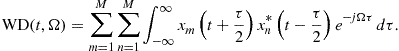
Besides the auto-terms
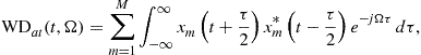
the Wigner distribution contains a significant number of cross-terms,

Usually, they are not desirable in the time-frequency signal analysis. Cross-terms can mask the presence of auto-terms, which makes the Wigner distribution unsuitable for the time-frequency analysis of signals.
For a two-component signal with auto-terms located around ![]() and
and ![]() (see Figure 3.14) the oscillatory cross-terms are located around
(see Figure 3.14) the oscillatory cross-terms are located around ![]() .
.
Example 10
For two-component signal of the form
![]()
we have

where the first and second terms represent auto-terms while the third term is a cross-term. Note that the cross-term is oscillatory in both directions. The oscillation rate along the time axis is proportional to the frequency distance between components ![]() , while the oscillation rate along frequency axis is proportional to the distance in time of components,
, while the oscillation rate along frequency axis is proportional to the distance in time of components, ![]() . The oscillatory nature of cross-terms will be used for their suppression.
. The oscillatory nature of cross-terms will be used for their suppression.

3.03.3.2.9 Inner interferences in the Wigner distribution
Another serious drawback of the Wigner distribution is in the presence of inner interferences for non-linear FM signals. Using the Taylor series expansion of the signal’s ![]() phase we get:
phase we get:

where ![]() is the term introducing interferences. The analytic form of this term can be obtained by using the stationary phase approximation.
is the term introducing interferences. The analytic form of this term can be obtained by using the stationary phase approximation.
For example, let us consider a cubic phase signal (quadratic frequency modulated) with Gaussian amplitude
![]()
The Wigner distribution value is:
![]()
The stationary phase points are
![]()
or ![]() and
and ![]() for
for ![]() , and
, and
![]()
The resulting stationary phase approximation of the Wigner distribution is obtained by summing contribution from both stationary phase points, ![]() and
and ![]() , as
, as
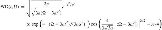
for ![]() and
and ![]() for
for ![]() . For
. For ![]() , significant oscillatory values are up to
, significant oscillatory values are up to ![]() , since the attenuation in frequency is
, since the attenuation in frequency is ![]() . Note that this is not in agreement with the expectation that the instantaneous bandwidth
. Note that this is not in agreement with the expectation that the instantaneous bandwidth ![]() , calculated according to (3.64), is small for a large
, calculated according to (3.64), is small for a large ![]() .
.
Note that the stationary phase is an approximation, producing accurate results for large arguments. In this case, exact Wigner distribution almost coincides with this approximation, already for ![]() as presented in Figure 3.15.
as presented in Figure 3.15.
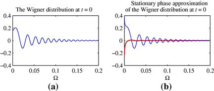
Figure 3.15 Stationary phase approximation of the Wigner distribution of a cubic-phase signal. The approximation error is presented with thick red line. (For interpretation of the references to color in this Figure 3.15 legend, the reader is referred to the web version of this book.)
If these terms are not reduced, they can reduce the accuracy of the time-frequency representation of a signal.
3.03.3.2.10 Pseudo and smoothed Wigner distribution
In practical realizations of the Wigner distribution, we are constrained with a finite time lag ![]() . A pseudo form of the Wigner distribution is then used [2,9,10,13,18,23,35]. It is defined as
. A pseudo form of the Wigner distribution is then used [2,9,10,13,18,23,35]. It is defined as
![]() (3.69)
(3.69)
where window ![]() localizes the considered lag interval. If
localizes the considered lag interval. If ![]() , the pseudo Wigner distribution satisfies the time marginal property. Note that the pseudo Wigner distribution is smoothed in the frequency direction with respect to the Wigner distribution
, the pseudo Wigner distribution satisfies the time marginal property. Note that the pseudo Wigner distribution is smoothed in the frequency direction with respect to the Wigner distribution
![]()
where ![]() is a FT of
is a FT of ![]() . The pseudo Wigner distribution example for multi-component signals is presented in Figure 3.16. Mono-component case with sinusoidally frequency modulated signal is presented in Figure 3.17. Note that significant inner interferences are present.
. The pseudo Wigner distribution example for multi-component signals is presented in Figure 3.16. Mono-component case with sinusoidally frequency modulated signal is presented in Figure 3.17. Note that significant inner interferences are present.
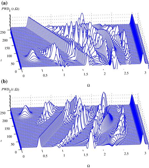
Figure 3.16 The pseudo Wigner distribution of signals from Figure 3.1.

Figure 3.17 The pseudo Wigner distribution for a sinusoidally frequency modulated signal. A narrow window (left) and a wide window (right).
In order to reduce the interferences in the Wigner distribution, it is sometimes smoothed not only in the frequency axis direction, but also in time, by using time-smoothing window ![]() . This form is called the smoothed Wigner distribution
. This form is called the smoothed Wigner distribution
![]() (3.70)
(3.70)
The smoothed Wigner distribution with
![]()
is equal to the spectrogram with window ![]() if
if ![]() . This smoothed Wigner distribution is always positive.
. This smoothed Wigner distribution is always positive.
3.03.3.2.11 Discrete pseudo Wigner distribution
The pseudo Wigner distribution of a discrete-time signal, with a finite length lag window, is given by
 (3.71)
Note that the pseudo Wigner distribution is periodic in ![]() with period
with period ![]() . The signal should be sampled at a twice higher sampling rate than it is required by the sampling theorem,
. The signal should be sampled at a twice higher sampling rate than it is required by the sampling theorem, ![]() . Thus, with the same lag window length the pseudo Wigner distribution will have twice more samples than the STFT. In order to produce an unbiased approximation of the analog form (3.69), the sampled signal in (3.71) should be formed as
. Thus, with the same lag window length the pseudo Wigner distribution will have twice more samples than the STFT. In order to produce an unbiased approximation of the analog form (3.69), the sampled signal in (3.71) should be formed as ![]() .
.
The discrete time and frequency form is given by

and may also be efficiently calculated by using the FFT routines. Note that discrete frequency ![]() is related to frequency index k as
is related to frequency index k as ![]() .
.
In order to avoid the need for oversampling, as well as to eliminate cross-terms between positive and negative frequency components in real signals, the real valued signals are usually transformed into their analytic forms ![]() , where
, where ![]() is the signal’s Hilbert transform. In the frequency domain
is the signal’s Hilbert transform. In the frequency domain ![]() , for
, for ![]() and
and ![]() for
for ![]() , while
, while ![]() , for
, for ![]() . Pseudo Wigner distribution is then calculated based on the analytic form of a signal. A STFT-based approach for creating the alias-free Wigner distribution will be also described later in the text.
. Pseudo Wigner distribution is then calculated based on the analytic form of a signal. A STFT-based approach for creating the alias-free Wigner distribution will be also described later in the text.
3.03.3.2.12 Wigner distribution based inversion and synthesis
In order to define an efficient algorithm for the synthesis of a signal with specified time-frequency distribution, we will restate the Wigner distribution inversion within the eigenvalue and eigenvectors decomposition framework. A discrete form of the Wigner distribution is defined by
 (3.72)
where we assume that the signal ![]() is time limited within
is time limited within ![]() . Inversion relation for the Wigner distribution reads
. Inversion relation for the Wigner distribution reads
After substitutions ![]() and
and ![]() we get
we get
 (3.73)
For cases when ![]() is not an integer, an appropriate interpolation is performed in order to calculate
is not an integer, an appropriate interpolation is performed in order to calculate ![]() .
.
Note that relation (3.73) is a discrete counterpart of the Wigner distribution inversion in analog domain, that reads:
![]()
By discretization of angular frequency ![]() and time
and time ![]() , with appropriate definition of discrete values, we easily obtain (3.73).
, with appropriate definition of discrete values, we easily obtain (3.73).
Introducing the notation,
 (3.74)
we get
![]() (3.75)
(3.75)
Matrix form of (3.75) reads
![]() (3.76)
(3.76)
where ![]() is a column vector whose elements are the signal values,
is a column vector whose elements are the signal values, ![]() is a row vector (Hermitian transpose of
is a row vector (Hermitian transpose of ![]() ), and
), and ![]() is a matrix with the elements
is a matrix with the elements ![]() , defined by (3.74).
, defined by (3.74).
The eigenvalue decomposition of ![]() reads
reads
 (3.77)
where ![]() are eigenvalues and
are eigenvalues and ![]() are corresponding eigenvectors of
are corresponding eigenvectors of ![]() . By comparing (3.76) and (3.77), it follows that the matrix with elements of form (3.74) can be decomposed by using only one non-zero eigenvalue. Note that the energy of the corresponding eigenvector is equal to 1, by definition
. By comparing (3.76) and (3.77), it follows that the matrix with elements of form (3.74) can be decomposed by using only one non-zero eigenvalue. Note that the energy of the corresponding eigenvector is equal to 1, by definition ![]() . By comparing (3.76) and (3.77), having in mind that there is only one non-zero eigenvalue
. By comparing (3.76) and (3.77), having in mind that there is only one non-zero eigenvalue ![]() , we have
, we have
![]()
and
 (3.78)
The eigenvector ![]() is equal to the signal vector
is equal to the signal vector ![]() , up to the constant amplitude and phase factor. Therefore, an eigenvalue decomposition of the matrix, formed according to (3.74), can be used to check if an arbitrary 2D function
, up to the constant amplitude and phase factor. Therefore, an eigenvalue decomposition of the matrix, formed according to (3.74), can be used to check if an arbitrary 2D function ![]() is a valid Wigner distribution.
is a valid Wigner distribution.
These relations can be used in signal synthesis. Assume that we have a given function ![]() , calculate (3.74) and perform eigenvalue decomposition (3.77). If the given function is the Wigner distribution of a signal it will result in one non-zero eigenvalue and corresponding eigenvector. If that is not the case then the first (largest) eigenvalue and corresponding eigenvector produce a signal such that its Wigner distribution will be the closest possible Wigner distribution (in the LMS sense) to the given arbitrary function
, calculate (3.74) and perform eigenvalue decomposition (3.77). If the given function is the Wigner distribution of a signal it will result in one non-zero eigenvalue and corresponding eigenvector. If that is not the case then the first (largest) eigenvalue and corresponding eigenvector produce a signal such that its Wigner distribution will be the closest possible Wigner distribution (in the LMS sense) to the given arbitrary function ![]() . This conclusion follows from the eigenvalue/eigenvectors decomposition properties.
. This conclusion follows from the eigenvalue/eigenvectors decomposition properties.
3.03.3.3 Ambiguity function
To analyze auto-terms and cross-terms, the well-known ambiguity function can be used as well. It is defined as:
![]() (3.79)
(3.79)
It is already a classical tool in optics as well as in radar and sonar signal analysis.
The ambiguity function and the Wigner distribution form a two-dimensional FT pair
![]()
Consider a signal whose components are limited in time to
![]()
In the ambiguity ![]() domain we have
domain we have ![]() only for
only for
![]()
It means that ![]() is located within
is located within ![]() , i.e., around the
, i.e., around the ![]() -axis independently of the signal’s position
-axis independently of the signal’s position ![]() . Cross-term between signal’s mth and nth component is located within
. Cross-term between signal’s mth and nth component is located within ![]() . It is dislocated from
. It is dislocated from ![]() for two-components that do not occur simultaneously, i.e., when
for two-components that do not occur simultaneously, i.e., when ![]() .
.
From the frequency domain definition of the Wigner distribution a corresponding ambiguity function form follows:
![]() (3.80)
(3.80)
From this form we can conclude that the auto-terms of the components, limited in frequency to ![]() only for
only for ![]() , are located in the ambiguity domain around
, are located in the ambiguity domain around ![]() -axis within the region
-axis within the region ![]() . The cross-terms are within
. The cross-terms are within
![]()
where ![]() and
and ![]() are the frequencies around which the FT of each component lies.
are the frequencies around which the FT of each component lies.
Therefore, all auto-terms are located along and around the ambiguity domain axis. The cross-terms, for the components which do not overlap in the time and frequency, simultaneously, are dislocated from the ambiguity axes, Figure 3.18. This property will be used in the definition of the reduced interference time-frequency distributions.

The ambiguity function of a four-component signal consisting of two Gaussian pulses, one sinusoidal and one linear frequency modulated component is presented in Figure 3.19.
Example 11
Let us consider signals of the form
The ambiguity function of ![]() is
is
![]()
while the ambiguity function of two-component signal ![]() is
is

In the ambiguity domain ![]() auto-terms are located around
auto-terms are located around ![]() while cross-terms are located around
while cross-terms are located around ![]() and
and ![]() as presented in Figure 3.18.
as presented in Figure 3.18.
Example 12
Show that the second order moment of the signal
![]()
may be calculated based on the signal’s and the Fourier transform’s second order moments and the joint first order moment.
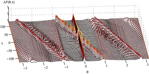
Figure 3.19 Ambiguity function of the signal from Figure 3.1.
For signal ![]() , the Wigner distribution is obtained by linear coordinate transformation of the Wigner distribution of a signal
, the Wigner distribution is obtained by linear coordinate transformation of the Wigner distribution of a signal ![]() ,
,
![]() (3.81)
(3.81)
The coordinate transformation matrix has the form
with ![]() , and D being related to
, and D being related to ![]() by the expressions in the transformation matrix.
by the expressions in the transformation matrix.
The second order moment of ![]() is
is
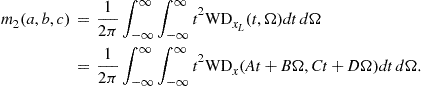
With a change of variables ![]() and
and ![]() , having in mind that the transformation is unitary,
, having in mind that the transformation is unitary, ![]() ,
,
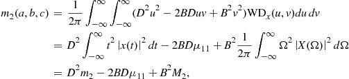 (3.82)
where ![]() could be calculated as
could be calculated as ![]() and
and
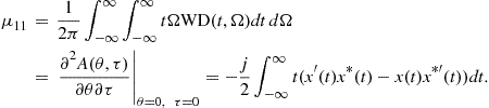
This relation is useful for multiparameter optimization in order to find time-frequency representation (with distribution coordinate transformation) that would produce the best concentrated signal, with minimal moment ![]() . Similar relation was obtained in the local polynomial Fourier transform analysis. A special case, that reduces to the time-frequency plane rotation with
. Similar relation was obtained in the local polynomial Fourier transform analysis. A special case, that reduces to the time-frequency plane rotation with ![]() and
and ![]() is used in practice by fractional Fourier transforms [8,33].
is used in practice by fractional Fourier transforms [8,33].
3.03.3.4 Cohen class of distributions
Time and frequency marginal properties (3.42) and (3.43) may be considered as the projections of the distribution ![]() along the time and frequency axes, i.e., as the Radon transform of
along the time and frequency axes, i.e., as the Radon transform of ![]() along these two directions. It is known that the FT of the projection of a two-dimensional function on a given line is equal to the value of the two-dimensional FT of
along these two directions. It is known that the FT of the projection of a two-dimensional function on a given line is equal to the value of the two-dimensional FT of ![]() , denoted by
, denoted by ![]() , along the same direction (inverse Radon transform property). Therefore, if
, along the same direction (inverse Radon transform property). Therefore, if ![]() satisfies marginal properties then any other function having two-dimensional FT equals to
satisfies marginal properties then any other function having two-dimensional FT equals to ![]() along the axes lines
along the axes lines ![]() and
and ![]() , and arbitrary values elsewhere, will satisfy marginal properties, Figure 3.20.
, and arbitrary values elsewhere, will satisfy marginal properties, Figure 3.20.