
3.09.7 Comparing the performance of cooperative strategies
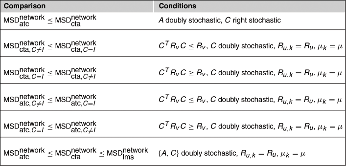
Using the expressions just derived for the MSD of the network, we can compare the performance of various cooperative and non-cooperative strategies. Table 9.6 further ahead summarizes the results derived in this section and the conditions under which they hold.
3.09.7.1 Comparing ATC and CTA strategies
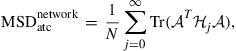
We first compare the performance of the adaptive ATC and CTA diffusion strategies (9.153) and (9.154) when they employ a doubly stochastic combination matrix ![]() . That is, let us consider the two scenarios:
. That is, let us consider the two scenarios:
![]() (9.332)
(9.332)
![]() (9.333)
(9.333)
where ![]() is now assumed to be doubly stochastic, i.e.,
is now assumed to be doubly stochastic, i.e.,
![]() (9.334)
(9.334)
with its rows and columns adding up to one. For example, these conditions are satisfied when ![]() is left stochastic and symmetric. Then, expressions (9.307) and (9.309) give:
is left stochastic and symmetric. Then, expressions (9.307) and (9.309) give:
![]() (9.335)
(9.335)
![]() (9.336)
(9.336)
where
![]() (9.337)
(9.337)
Following [18], introduce the auxiliary nonnegative-definite matrix
![]() (9.338)
(9.338)
Then, it is immediate to verify from (9.306) that
 (9.339)
 (9.340)
so that
 (9.341)
Now, since ![]() is doubly stochastic, it also holds that the enlarged matrix
is doubly stochastic, it also holds that the enlarged matrix ![]() is doubly stochastic. Moreover, for any doubly stochastic matrix
is doubly stochastic. Moreover, for any doubly stochastic matrix ![]() and any nonnegative-definite matrix
and any nonnegative-definite matrix ![]() of compatible dimensions, it holds that (see part (f) of Theorem C.3):
of compatible dimensions, it holds that (see part (f) of Theorem C.3):
![]() (9.342)
(9.342)
Applying result (9.342) to (9.341) we conclude that
![]() (9.343)
(9.343)
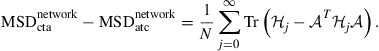
so that the adaptive ATC strategy (9.153) outperforms the adaptive CTA strategy (9.154) for doubly stochastic combination matrices ![]() .
.
3.09.7.2 Comparing strategies with and without information exchange
We now examine the effect of information exchange ![]() on the performance of the adaptive ATC and CTA diffusion strategies (9.153) and (9.154) under conditions (9.310)–(9.312) for uniform data profile.
on the performance of the adaptive ATC and CTA diffusion strategies (9.153) and (9.154) under conditions (9.310)–(9.312) for uniform data profile.
3.09.7.2.1 CTA Strategies
We start with the adaptive CTA strategy (9.154), and consider two scenarios with and without information exchange. These scenarios correspond to the following selections in the general description (9.201)–(9.203):
![]() (9.344)
(9.344)
![]() (9.345)
(9.345)
Then, expressions (9.322) and (9.323) give:
![]() (9.346)
(9.346)
![]() (9.347)
(9.347)
where the matrix ![]() is defined by (9.319). Note that
is defined by (9.319). Note that ![]() , so we denote them simply by
, so we denote them simply by ![]() in the derivation that follows. Then, from expression (9.306) for the network MSD we get:
in the derivation that follows. Then, from expression (9.306) for the network MSD we get:
 (9.348)
It follows that the difference in performance between both CTA implementations depends on how the matrices ![]() and
and ![]() compare to each other:
compare to each other:
![]() (9.349)
(9.349)
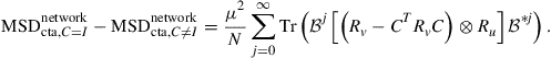
so that a CTA implementation with information exchange performs better than a CTA implementation without information exchange. Note that the condition on ![]() corresponds to requiring
corresponds to requiring
![]() (9.350)
(9.350)
which can be interpreted to mean that the cooperation matrix ![]() should be such that it does not amplify the effect of measurement noise. For example, this situation occurs when the noise profile is uniform across the network, in which case
should be such that it does not amplify the effect of measurement noise. For example, this situation occurs when the noise profile is uniform across the network, in which case ![]() . This is because it would then hold that
. This is because it would then hold that
![]() (9.351)
(9.351)
in view of the fact that ![]() since
since ![]() is doubly stochastic (cf. property (e) in Lemma C.3).
is doubly stochastic (cf. property (e) in Lemma C.3).
![]() (9.352)
(9.352)
so that a CTA implementation without information exchange performs better than a CTA implementation with information exchange. In this case, the condition on ![]() indicates that the combination matrix
indicates that the combination matrix ![]() ends up amplifying the effect of noise.
ends up amplifying the effect of noise.
3.09.7.2.2 ATC Strategies
We can repeat the argument for the adaptive ATC strategy (9.153), and consider two scenarios with and without information exchange. These scenarios correspond to the following selections in the general description (9.201)–(9.203):
![]() (9.353)
(9.353)
![]() (9.354)
(9.354)
Then, expressions (9.322) and (9.323) give:
![]() (9.355)
(9.355)
![]() (9.356)
(9.356)
Note again that ![]() , so we denote them simply by
, so we denote them simply by ![]() . Then,
. Then,
 (9.357)
It again follows that the difference in performance between both ATC implementations depends on how the matrices ![]() and
and ![]() compare to each other and we obtain:
compare to each other and we obtain:
![]() (9.358)
(9.358)
and
![]() (9.359)
(9.359)
3.09.7.3 Comparing diffusion strategies with the non-cooperative strategy
We now compare the performance of the adaptive CTA strategy (9.154) to the non-cooperative LMS strategy (9.207) assuming conditions (9.310)–(9.312) for uniform data profile. These scenarios correspond to the following selections in the general description (9.201)–(9.203):
![]() (9.360)
(9.360)
![]() (9.361)
(9.361)
where ![]() is further assumed to be doubly stochastic (along with
is further assumed to be doubly stochastic (along with ![]() ) so that
) so that
![]() (9.362)
(9.362)
Then, expressions (9.322) and (9.323) give:
![]() (9.363)
(9.363)
![]() (9.364)
(9.364)
Now recall that
![]() (9.365)
(9.365)
so that, using the Kronecker product property (9.317),
 (9.366)
Then,
 (9.367)
Let us examine the difference:
 (9.368)
Now, due to the even power, it always holds that ![]() . Moreover, since
. Moreover, since ![]() and
and ![]() are doubly stochastic, it follows that
are doubly stochastic, it follows that ![]() is also doubly stochastic. Therefore, the matrix
is also doubly stochastic. Therefore, the matrix ![]() is nonnegative-definite as well (cf. property (e) of Lemma C.3). It follows that
is nonnegative-definite as well (cf. property (e) of Lemma C.3). It follows that
![]() (9.369)
(9.369)
But since ![]() , we conclude from (9.367) that
, we conclude from (9.367) that
![]() (9.370)
(9.370)
This is because for any two Hermitian nonnegative-definite matrices ![]() and
and ![]() of compatible dimensions, it holds that
of compatible dimensions, it holds that ![]() ; indeed if we factor
; indeed if we factor ![]() with
with ![]() full rank, then
full rank, then ![]() . We conclude from this analysis that adaptive CTA diffusion performs better than non-cooperative LMS under uniform data profile conditions and doubly stochastic
. We conclude from this analysis that adaptive CTA diffusion performs better than non-cooperative LMS under uniform data profile conditions and doubly stochastic ![]() . If we refer to the earlier result (9.343), we conclude that the following relation holds:
. If we refer to the earlier result (9.343), we conclude that the following relation holds:
![]() (9.371)
(9.371)
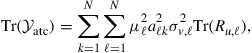
Table 9.6 lists the comparison results derived in this section and lists the conditions under which the conclusions hold.
3.09.8 Selecting the combination weights
The adaptive diffusion strategy (9.201)–(9.203) employs combination weights ![]() or, equivalently, combination matrices
or, equivalently, combination matrices ![]() , where
, where ![]() and
and ![]() are left-stochastic matrices and
are left-stochastic matrices and ![]() is a right-stochastic matrix. There are several ways by which these matrices can be selected. In this section, we describe constructions that result in left-stochastic or doubly-stochastic combination matrices,
is a right-stochastic matrix. There are several ways by which these matrices can be selected. In this section, we describe constructions that result in left-stochastic or doubly-stochastic combination matrices, ![]() . When a right-stochastic combination matrix is needed, such as
. When a right-stochastic combination matrix is needed, such as ![]() , then it can be obtained by transposition of the left-stochastic constructions shown below.
, then it can be obtained by transposition of the left-stochastic constructions shown below.
3.09.8.1 Constant combination weights
Table 9.7 lists a couple of common choices for selecting constant combination weights for a network with ![]() nodes. Several of these constructions appeared originally in the literature on graph theory. In the table, the symbol
nodes. Several of these constructions appeared originally in the literature on graph theory. In the table, the symbol ![]() denotes the degree of node
denotes the degree of node ![]() , which refers to the size of its neighborhood. Likewise, the symbol
, which refers to the size of its neighborhood. Likewise, the symbol ![]() refers to the maximum degree across the network, i.e.,
refers to the maximum degree across the network, i.e.,
![]() (9.372)
(9.372)
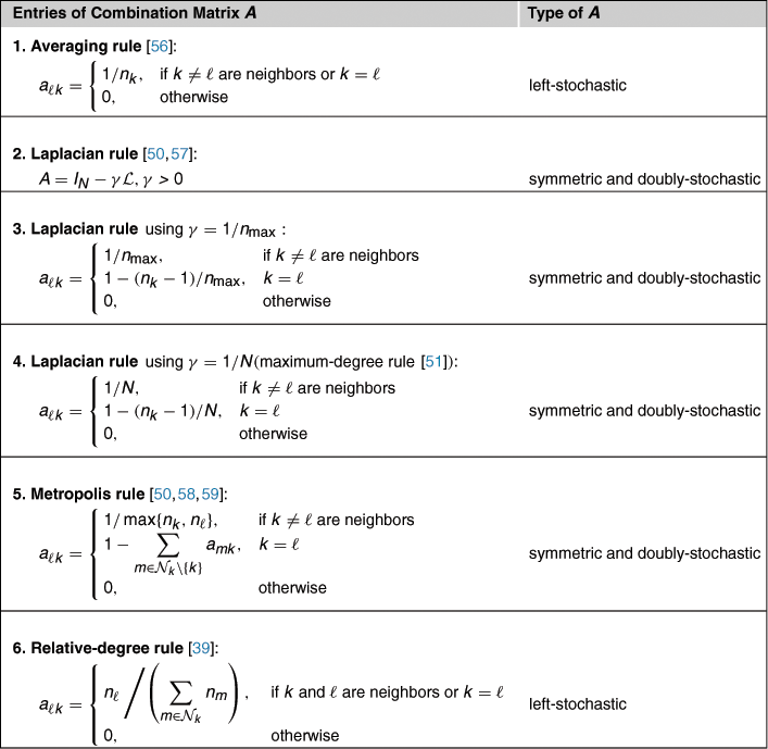
The Laplacian rule, which appears in the second line of the table, relies on the use of the Laplacian matrix ![]() of the network and a positive scalar
of the network and a positive scalar ![]() . The Laplacian matrix is defined by (9.574) in Appendix B, namely, it is a symmetric matrix whose entries are constructed as follows [60–62]:
. The Laplacian matrix is defined by (9.574) in Appendix B, namely, it is a symmetric matrix whose entries are constructed as follows [60–62]:
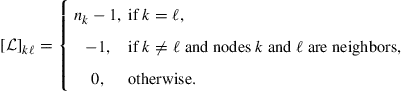 (9.373)
The Laplacian rule can be reduced to other forms through the selection of the positive parameter ![]() . One choice is
. One choice is ![]() while another choice is
while another choice is ![]() and leads to the maximum-degree rule. Obviously, it always holds that
and leads to the maximum-degree rule. Obviously, it always holds that ![]() so that
so that ![]() . Therefore, the choice
. Therefore, the choice ![]() ends up assigning larger weights to neighbors than the choice
ends up assigning larger weights to neighbors than the choice ![]() . The averaging rule in the first row of the table is one of the simplest combination rules whereby nodes simply average data from their neighbors.
. The averaging rule in the first row of the table is one of the simplest combination rules whereby nodes simply average data from their neighbors.
In the constructions in Table 9.7, the values of the weights ![]() are largely dependent on the degree of the nodes. In this way, the number of connections that each node has influences the combination weights with its neighbors. While such selections may be appropriate in some applications, they can nevertheless degrade the performance of adaptation over networks [63]. This is because such weighting schemes ignore the noise profile across the network. And since some nodes can be noisier than others, it is not sufficient to rely solely on the amount of connectivity that nodes have to determine the combination weights to their neighbors. It is important to take into account the amount of noise that is present at the nodes as well. Therefore, designing combination rules that are aware of the variation in noise profile across the network is an important task. It is also important to devise strategies that are able to adapt these combination weights in response to variations in network topology and data statistical profile. For this reason, following [64,65], we describe in the next subsection one adaptive procedure for adjusting the combination weights. This procedure allows the network to assign more or less relevance to nodes according to the quality of their data.
are largely dependent on the degree of the nodes. In this way, the number of connections that each node has influences the combination weights with its neighbors. While such selections may be appropriate in some applications, they can nevertheless degrade the performance of adaptation over networks [63]. This is because such weighting schemes ignore the noise profile across the network. And since some nodes can be noisier than others, it is not sufficient to rely solely on the amount of connectivity that nodes have to determine the combination weights to their neighbors. It is important to take into account the amount of noise that is present at the nodes as well. Therefore, designing combination rules that are aware of the variation in noise profile across the network is an important task. It is also important to devise strategies that are able to adapt these combination weights in response to variations in network topology and data statistical profile. For this reason, following [64,65], we describe in the next subsection one adaptive procedure for adjusting the combination weights. This procedure allows the network to assign more or less relevance to nodes according to the quality of their data.
3.09.8.2 Optimizing the combination weights
Ideally, we would like to select ![]() combination matrices
combination matrices ![]() in order to minimize the network MSD given by (9.302) or (9.306). In [18], the selection of the combination weights was formulated as the following optimization problem:
in order to minimize the network MSD given by (9.302) or (9.306). In [18], the selection of the combination weights was formulated as the following optimization problem:
 (9.374)
We can pursue a numerical solution to (9.374) in order to search for optimal combination matrices, as was done in [18]. Here, however, we are interested in an adaptive solution that becomes part of the learning process so that the network can adapt the weights on the fly in response to network conditions. We illustrate an approximate approach from [64,65] that leads to one adaptive solution that performs reasonably well in practice.
We illustrate the construction by considering the ATC strategy (9.158) without information exchange where ![]()
![]() , and
, and ![]() . In this case, recursions (9.204)–(9.206) take the form:
. In this case, recursions (9.204)–(9.206) take the form:
![]() (9.375)
(9.375)
![]() (9.376)
(9.376)
and, from (9.306), the corresponding network MSD performance is:
 (9.377)
where
![]() (9.378)
(9.378)
![]() (9.379)
(9.379)
![]() (9.380)
(9.380)
![]() (9.381)
(9.381)
![]() (9.382)
(9.382)
![]() (9.383)
(9.383)
Minimizing the MSD expression (9.377) over left-stochastic matrices ![]() is generally non-trivial. We pursue an approximate solution.
is generally non-trivial. We pursue an approximate solution.
To begin with, for compactness of notation, let ![]() denote the spectral radius of the
denote the spectral radius of the ![]() block matrix
block matrix ![]() :
:
![]() (9.384)
(9.384)
We already know, in view of the mean and mean-square stability of the network, that ![]() . Now, consider the series that appears in (9.377) and whose trace we wish to minimize over
. Now, consider the series that appears in (9.377) and whose trace we wish to minimize over ![]() . Note that its block maximum norm can be bounded as follows:
. Note that its block maximum norm can be bounded as follows:
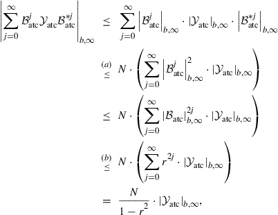 (9.385)
where for step (b) we use result (9.602) to conclude that
 (9.386)
To justify step (a), we use result (9.584) to relate the norms of ![]() and its complex conjugate,
and its complex conjugate, ![]() , as
, as
![]() (9.387)
(9.387)
Expression (9.385) then shows that the norm of the series appearing in (9.377) is bounded by a scaled multiple of the norm of ![]() , and the scaling constant is independent of
, and the scaling constant is independent of ![]() . Using property (9.586) we conclude that there exists a positive constant
. Using property (9.586) we conclude that there exists a positive constant ![]() , also independent of
, also independent of ![]() , such that
, such that
 (9.388)
Therefore, instead of attempting to minimize the trace of the series, the above result motivates us to minimize an upper bound to the trace. Thus, we consider the alternative problem of minimizing the first term of the series (9.377), namely,
 (9.389)
Using (9.379), the trace of ![]() can be expressed in terms of the combination coefficients as follows:
can be expressed in terms of the combination coefficients as follows:
 (9.390)
so that problem (9.389) can be decoupled into ![]() separate optimization problems of the form:
separate optimization problems of the form:
 (9.391)
With each node ![]() , we associate the following nonnegative noise-data-dependent measure:
, we associate the following nonnegative noise-data-dependent measure:
![]() (9.392)
(9.392)
This measure amounts to scaling the noise variance at node ![]() by
by ![]() and by the power of the regression data (measured through the trace of its covariance matrix). We shall refer to
and by the power of the regression data (measured through the trace of its covariance matrix). We shall refer to ![]() as the noise-data variance product (or variance product, for simplicity) at node
as the noise-data variance product (or variance product, for simplicity) at node ![]() . Then, the solution of (9.391) is given by:
. Then, the solution of (9.391) is given by:
 (9.393)
We refer to this combination rule as the relative-variance combination rule [64]; it leads to a left-stochastic matrix ![]() . In this construction, node
. In this construction, node ![]() combines the intermediate estimates
combines the intermediate estimates ![]() from its neighbors in (9.376) in proportion to the inverses of their variance products,
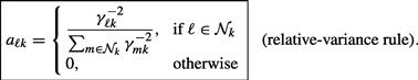
from its neighbors in (9.376) in proportion to the inverses of their variance products, ![]() . The result is physically meaningful. Nodes with smaller variance products will generally be given larger weights. In comparison, the following relative-degree-variance rule was proposed in [18] (a typo appears in Table III in [18], where the noise variances appear written in the table instead of their inverses):
. The result is physically meaningful. Nodes with smaller variance products will generally be given larger weights. In comparison, the following relative-degree-variance rule was proposed in [18] (a typo appears in Table III in [18], where the noise variances appear written in the table instead of their inverses):
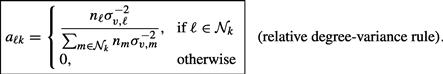 (9.394)
This second form also leads to a left-stochastic combination matrix ![]() . However, rule (9.394) does not take into account the covariance matrices of the regression data across the network. Observe that in the special case when the step-sizes, regression covariance matrices, and noise variances are uniform across the network, i.e.,
. However, rule (9.394) does not take into account the covariance matrices of the regression data across the network. Observe that in the special case when the step-sizes, regression covariance matrices, and noise variances are uniform across the network, i.e., ![]() ,
, ![]() and
and ![]() for all
for all ![]() , expression (9.393) reduces to the simple averaging rule (first line of Table 9.7). In contrast, expression (9.394) reduces the relative degree rule (last line of Table 9.7).
, expression (9.393) reduces to the simple averaging rule (first line of Table 9.7). In contrast, expression (9.394) reduces the relative degree rule (last line of Table 9.7).
3.09.8.3 Adaptive combination weights
To evaluate the combination weights (9.393), the nodes need to know the variance products, ![]() , of their neighbors. According to (9.392), the factors
, of their neighbors. According to (9.392), the factors ![]() are defined in terms of the noise variances,
are defined in terms of the noise variances, ![]() , and the regression covariance matrices,
, and the regression covariance matrices, ![]() , and these quantities are not known beforehand. The nodes only have access to realizations of
, and these quantities are not known beforehand. The nodes only have access to realizations of ![]() . We now describe one procedure that allows every node
. We now describe one procedure that allows every node ![]() to learn the variance products of its neighbors in an adaptive manner. Note that if a particular node
to learn the variance products of its neighbors in an adaptive manner. Note that if a particular node ![]() happens to belong to two neighborhoods, say, the neighborhood of node
happens to belong to two neighborhoods, say, the neighborhood of node ![]() and the neighborhood of node
and the neighborhood of node ![]() , then each of
, then each of ![]() and
and ![]() need to evaluate the variance product,
need to evaluate the variance product, ![]() , of node
, of node ![]() . The procedure described below allows each node in the network to estimate the variance products of its neighbors in a recursive manner.
. The procedure described below allows each node in the network to estimate the variance products of its neighbors in a recursive manner.
To motivate the algorithm, we refer to the ATC recursion (9.375), (9.376) and use the data model (9.208) to write for node ![]() :
:
![]() (9.395)
(9.395)
so that, in view of our earlier assumptions on the regression data and noise in Section 3.09.6.1, we obtain in the limit as ![]() :
:
![]() (9.396)
(9.396)
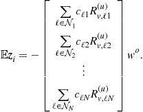
We can evaluate the limit on the right-hand side by using the steady-state result (9.284). Indeed, we select the vector ![]() in (9.284) to satisfy
in (9.284) to satisfy
![]() (9.397)
(9.397)
Then, from (9.284),
![]() (9.398)
(9.398)
Now recall from expression (9.379) for ![]() that for the ATC algorithm under consideration we have
that for the ATC algorithm under consideration we have
![]() (9.399)
(9.399)
so that the entries of ![]() depend on combinations of the squared step-sizes,
depend on combinations of the squared step-sizes, ![]() . This fact implies that the first term on the right-hand side of (9.396) depends on products of the form
. This fact implies that the first term on the right-hand side of (9.396) depends on products of the form ![]() ; these fourth-order factors can be ignored in comparison to the second-order factor
; these fourth-order factors can be ignored in comparison to the second-order factor ![]() for small step-sizes so that
for small step-sizes so that
 (9.400)
in terms of the desired variance product, ![]() . Using the following instantaneous approximation at node
. Using the following instantaneous approximation at node ![]() (where
(where ![]() is replaced by
is replaced by ![]() ):
):
![]() (9.401)
(9.401)
We can now motivate an algorithm that enables node ![]() to estimate the variance product,
to estimate the variance product, ![]() of its neighbor
of its neighbor ![]() . Thus, let
. Thus, let ![]() denote an estimate for
denote an estimate for ![]() that is computed by node
that is computed by node ![]() at time
at time ![]() . Then, one way to evaluate
. Then, one way to evaluate ![]() is through the recursion:
is through the recursion:
![]() (9.402)
(9.402)
where ![]() is a positive coefficient smaller than one. Note that under expectation, expression (9.402) becomes
is a positive coefficient smaller than one. Note that under expectation, expression (9.402) becomes
![]() (9.403)
(9.403)
so that in steady-state, as ![]() ,
,
![]() (9.404)
(9.404)
Hence, we obtain
![]() (9.405)
(9.405)
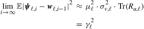
That is, the estimator ![]() converges on average close to the desired variance product
converges on average close to the desired variance product ![]() . In this way, we can replace the optimal weights (9.393) by the adaptive construction:
. In this way, we can replace the optimal weights (9.393) by the adaptive construction:
 (9.406)
Equations (9.402) and (9.406) provide one adaptive construction for the combination weights ![]() .
.
3.09.9 Diffusion with noisy information exchanges
The adaptive diffusion strategy (9.201)–(9.203) relies on the fusion of local information collected from neighborhoods through the use of combination matrices ![]() . In the previous section, we described several constructions for selecting such combination matrices. We also motivated and developed an adaptive scheme for the ATC mode of operation (9.375) and (9.376) that computes combination weights in a manner that is aware of the variation of the variance-product profile across the network. Nevertheless, in addition to the measurement noises
. In the previous section, we described several constructions for selecting such combination matrices. We also motivated and developed an adaptive scheme for the ATC mode of operation (9.375) and (9.376) that computes combination weights in a manner that is aware of the variation of the variance-product profile across the network. Nevertheless, in addition to the measurement noises ![]() at the individual nodes, we also need to consider the effect of perturbations that are introduced during the exchange of information among neighboring nodes. Noise over the communication links can be due to various factors including thermal noise and imperfect channel information. Studying the degradation in mean-square performance that results from these noisy exchanges can be pursued by straightforward extension of the mean-square analysis of Section 3.09.6, as we proceed to illustrate. Subsequently, we shall use the results to show how the combination weights can also be adapted in the presence of noisy exchange links.
at the individual nodes, we also need to consider the effect of perturbations that are introduced during the exchange of information among neighboring nodes. Noise over the communication links can be due to various factors including thermal noise and imperfect channel information. Studying the degradation in mean-square performance that results from these noisy exchanges can be pursued by straightforward extension of the mean-square analysis of Section 3.09.6, as we proceed to illustrate. Subsequently, we shall use the results to show how the combination weights can also be adapted in the presence of noisy exchange links.
3.09.9.1 Noise sources over exchange links
To model noisy links, we introduce an additive noise component into each of the steps of the diffusion strategy (9.201)–(9.203) during the operations of information exchange among the nodes. The notation becomes a bit cumbersome because we need to account for both the source and destination of the information that is being exchanged. For example, the same signal ![]() that is generated by node
that is generated by node ![]() will be broadcast to all the neighbors of node
will be broadcast to all the neighbors of node ![]() . When this is done, a different noise will interfere with the exchange of
. When this is done, a different noise will interfere with the exchange of ![]() over each of the edges that link node
over each of the edges that link node ![]() to its neighbors. Thus, we will need to use a notation of the form
to its neighbors. Thus, we will need to use a notation of the form ![]() , with two subscripts
, with two subscripts ![]() and
and ![]() , to indicate that this is the noisy version of
, to indicate that this is the noisy version of ![]() that is received by node
that is received by node ![]() from node
from node ![]() . The subscript
. The subscript ![]() indicates that
indicates that ![]() is the source and
is the source and ![]() is the sink, i.e., information is moving from
is the sink, i.e., information is moving from ![]() to
to ![]() . For the reverse situation where information flows from node
. For the reverse situation where information flows from node ![]() to
to ![]() , we would use instead the subscript
, we would use instead the subscript ![]() .
.
With this notation in mind, we model the noisy data received by node ![]() from its neighbor
from its neighbor ![]() as follows:
as follows:
![]() (9.407)
(9.407)
![]() (9.408)
(9.408)
![]() (9.409)
(9.409)
![]() (9.410)
(9.410)
where ![]() , and
, and ![]() are vector noise signals, and
are vector noise signals, and ![]() is a scalar noise signal. These are the noise signals that perturb exchanges over the edge linking source
is a scalar noise signal. These are the noise signals that perturb exchanges over the edge linking source ![]() to sink
to sink ![]() (i.e., for data sent from node
(i.e., for data sent from node ![]() to node
to node ![]() ). The superscripts
). The superscripts ![]() in each case refer to the variable that these noises perturb. Figure 9.14 illustrates the various noise sources that perturb the exchange of information from node
in each case refer to the variable that these noises perturb. Figure 9.14 illustrates the various noise sources that perturb the exchange of information from node ![]() to node
to node ![]() . The figure also shows the measurement noises
. The figure also shows the measurement noises ![]() that exist locally at the nodes in view of the data model (9.208).
that exist locally at the nodes in view of the data model (9.208).

Figure 9.14 Additive noise sources perturb the exchange of information from node ![]() to node
to node ![]() . The subscript
. The subscript ![]() in this illustration indicates that
in this illustration indicates that ![]() is the source node and
is the source node and ![]() is the sink node so that information is flowing from
is the sink node so that information is flowing from ![]() to
to ![]() .
.
We assume that the following noise signals, which influence the data received by node ![]() ,
,
![]() (9.411)
(9.411)
are temporally white and spatially independent random processes with zero mean and variances or covariances given by
![]() (9.412)
(9.412)
Obviously, the quantities
![]() (9.413)
(9.413)
are all zero if ![]() or when
or when ![]() . We further assume that the noise processes (9.411) are independent of each other and of the regression data
. We further assume that the noise processes (9.411) are independent of each other and of the regression data ![]() for all
for all ![]() and
and ![]() .
.
3.09.9.2 Error recursion
Using the perturbed data (9.407)–(9.410), the adaptive diffusion strategy (9.201)–(9.203) becomes
![]() (9.414)
(9.414)
![]() (9.415)
(9.415)
![]() (9.416)
(9.416)
Observe that the perturbed quantities ![]() , with subscripts
, with subscripts ![]() , appear in (9.414)–(9.416) in place of the original quantities
, appear in (9.414)–(9.416) in place of the original quantities ![]() that appear in (9.201)–(9.203). This is because these quantities are now subject to exchange noises. As before, we are still interested in examining the evolution of the weight-error vectors:
that appear in (9.201)–(9.203). This is because these quantities are now subject to exchange noises. As before, we are still interested in examining the evolution of the weight-error vectors:
![]() (9.417)
(9.417)
For this purpose, we again introduce the following ![]() block vector, whose entries are of size
block vector, whose entries are of size ![]() each:
each:
 (9.418)
and proceed to determine a recursion for its evolution over time. The arguments are largely similar to what we already did before in Section 3.09.6.3 and, therefore, we shall emphasize the differences that arise. The main deviation is that we now need to account for the presence of the new noise signals; they will contribute additional terms to the recursion for ![]() —see (9.442) further ahead. We may note that some studies on the effect of imperfect data exchanges on the performance of adaptive diffusion algorithms are considered in [66–68]. These earlier investigations were limited to particular cases in which only noise in the exchange of
—see (9.442) further ahead. We may note that some studies on the effect of imperfect data exchanges on the performance of adaptive diffusion algorithms are considered in [66–68]. These earlier investigations were limited to particular cases in which only noise in the exchange of ![]() was considered (as in (9.407)), in addition to setting
was considered (as in (9.407)), in addition to setting ![]() (in which case there is no exchange of
(in which case there is no exchange of ![]() ), and by focusing on the CTA case for which
), and by focusing on the CTA case for which ![]() . Here, we consider instead the general case that accounts for the additional sources of imperfections shown in (9.408)–(9.410), in addition to the general diffusion strategy (9.201)–(9.203) with combination matrices
. Here, we consider instead the general case that accounts for the additional sources of imperfections shown in (9.408)–(9.410), in addition to the general diffusion strategy (9.201)–(9.203) with combination matrices ![]() .
.
To begin with, we introduce the aggregate ![]() zero-mean noise signals:
zero-mean noise signals:
![]() (9.419)
(9.419)
These noises represent the aggregate effect on node ![]() of all exchange noises from the neighbors of node
of all exchange noises from the neighbors of node ![]() while exchanging the estimates
while exchanging the estimates ![]() during the two combination steps (9.201) and (9.203). The
during the two combination steps (9.201) and (9.203). The ![]() covariance matrices of these noises are given by
covariance matrices of these noises are given by
![]() (9.420)
(9.420)
These expressions aggregate the exchange noise covariances in the neighborhood of node ![]() ; the covariances are scaled by the squared coefficients
; the covariances are scaled by the squared coefficients ![]() . We collect these noise signals, and their covariances, from across the network into
. We collect these noise signals, and their covariances, from across the network into ![]() block vectors and
block vectors and ![]() block diagonal matrices as follows:
block diagonal matrices as follows:
![]() (9.421)
(9.421)
![]() (9.422)
(9.422)
![]() (9.423)
(9.423)
![]() (9.424)
(9.424)
We further introduce the following scalar zero-mean noise signal:
![]() (9.425)
(9.425)
whose variance is
![]() (9.426)
(9.426)
In the absence of exchange noises for the data ![]() , the signal
, the signal ![]() would coincide with the measurement noise
would coincide with the measurement noise ![]() . Expression (9.425) is simply a reflection of the aggregate effect of the noises in exchanging
. Expression (9.425) is simply a reflection of the aggregate effect of the noises in exchanging ![]() on node
on node ![]() . Indeed, starting from the data model (9.208) and using (9.409) and (9.410), we can easily verify that the noisy data
. Indeed, starting from the data model (9.208) and using (9.409) and (9.410), we can easily verify that the noisy data ![]() are related via:
are related via:
![]() (9.427)
(9.427)
We also define (compare with (9.234) and (9.235) and note that we are now using the perturbed regression vectors ![]() ):
):
![]() (9.428)
(9.428)
![]() (9.429)
(9.429)
It holds that
![]() (9.430)
(9.430)
where
 (9.431)
When there is no noise during the exchange of the regression data, i.e., when ![]() , the expressions for
, the expressions for ![]() reduce to expressions (9.234), (9.235), and (9.182) for
reduce to expressions (9.234), (9.235), and (9.182) for ![]() .
.
Likewise, we introduce (compare with (9.239)):
![]() (9.432)
(9.432)
![]() (9.433)
(9.433)
Compared with the earlier definition for ![]() in (9.239) when there is no noise over the exchange links, we see that we now need to account for the various noisy versions of the same regression vector
in (9.239) when there is no noise over the exchange links, we see that we now need to account for the various noisy versions of the same regression vector ![]() and the same signal
and the same signal ![]() . For instance, the vectors
. For instance, the vectors ![]() and
and ![]() would denote two noisy versions received by nodes
would denote two noisy versions received by nodes ![]() and
and ![]() for the same regression vector
for the same regression vector ![]() transmitted from node
transmitted from node ![]() . Likewise, the scalars
. Likewise, the scalars ![]() and
and ![]() would denote two noisy versions received by nodes
would denote two noisy versions received by nodes ![]() and
and ![]() for the same scalar
for the same scalar ![]() transmitted from node
transmitted from node ![]() . As a result, the quantity
. As a result, the quantity ![]() is not zero mean any longer (in contrast to
is not zero mean any longer (in contrast to ![]() , which had zero mean). Indeed, note that
, which had zero mean). Indeed, note that
 (9.434)
 (9.435)
Although we can continue our analysis by studying this general case in which the vectors ![]() do not have zero-mean (see [65,69]), we shall nevertheless limit our discussion in the sequel to the case in which there is no noise during the exchange of the regression data, i.e., we henceforth assume that:
do not have zero-mean (see [65,69]), we shall nevertheless limit our discussion in the sequel to the case in which there is no noise during the exchange of the regression data, i.e., we henceforth assume that:
![]() (9.436)
(9.436)
We maintain all other noise sources, which occur during the exchange of the weight estimates ![]() and the data
and the data ![]() . Under condition (9.436), we obtain
. Under condition (9.436), we obtain
![]() (9.437)
(9.437)
![]() (9.438)
(9.438)
![]() (9.439)
(9.439)
Then, the covariance matrix of each term ![]() is given by
is given by
![]() (9.440)
(9.440)
and the covariance matrix of ![]() is
is ![]() block diagonal with blocks of size
block diagonal with blocks of size ![]() :
:
![]() (9.441)
(9.441)
Now repeating the argument that led to (9.246) we arrive at the following recursion for the weight-error vector:
![]() (9.442)
(9.442)
For comparison purposes, we repeat recursion (9.246) here (recall that this recursion corresponds to the case when the exchanges over the links are not subject to noise):
![]() (9.443)
(9.443)
Comparing (9.442) and (9.443) we find that:
1. The covariance matrix ![]() in (9.443) is replaced by
in (9.443) is replaced by ![]() . Recall from (9.429) that
. Recall from (9.429) that ![]() contains the influence of the noises that arise during the exchange of the regression data, i.e., the
contains the influence of the noises that arise during the exchange of the regression data, i.e., the ![]() . But since we are now assuming that
. But since we are now assuming that ![]() , then
, then ![]() .
.
2. The term ![]() in (9.443) is replaced by
in (9.443) is replaced by ![]() . Recall from (9.432) that
. Recall from (9.432) that ![]() contains the influence of the noises that arise during the exchange of the measurement data and the regression data, i.e., the
contains the influence of the noises that arise during the exchange of the measurement data and the regression data, i.e., the ![]() .
.
3. Two new driving terms appear involving ![]() and
and ![]() . These terms reflect the influence of the noises during the exchange of the weight estimates
. These terms reflect the influence of the noises during the exchange of the weight estimates ![]() .
.
a. The term involving ![]() accounts for noise introduced at the information-exchange step (9.414) before adaptation.
accounts for noise introduced at the information-exchange step (9.414) before adaptation.
b. The term involving ![]() accounts for noise introduced during the adaptation step (9.415).
accounts for noise introduced during the adaptation step (9.415).
c. The term involving ![]() accounts for noise introduced at the information-exchange step (9.416) after adaptation.
accounts for noise introduced at the information-exchange step (9.416) after adaptation.
Therefore, since we are not considering noise during the exchange of the regression data, the weight-error recursion (9.442) simplifies to:
![]() (9.444)
(9.444)
where we used the fact that ![]() under these conditions.
under these conditions.
3.09.9.3 Convergence in the mean
Taking expectations of both sides of (9.444) we find that the mean error vector evolves according to the following recursion:
![]() (9.445)
(9.445)
with ![]() defined by (9.181). This is the same recursion encountered earlier in (9.248) during perfect data exchanges. Note that had we considered noises during the exchange of the regression data, then the vector
defined by (9.181). This is the same recursion encountered earlier in (9.248) during perfect data exchanges. Note that had we considered noises during the exchange of the regression data, then the vector ![]() in (9.444) would not be zero mean and the matrix
in (9.444) would not be zero mean and the matrix ![]() will have to be used instead of
will have to be used instead of ![]() . In that case, the recursion for
. In that case, the recursion for ![]() will be different from (9.445); i.e., the presence of noise during the exchange of regression data alters the dynamics of the mean error vector in an important way—see [65,69] for details on how to extend the arguments to this general case with a driving non-zero bias term. We can now extend Theorem 9.6.1 to the current scenario.
will be different from (9.445); i.e., the presence of noise during the exchange of regression data alters the dynamics of the mean error vector in an important way—see [65,69] for details on how to extend the arguments to this general case with a driving non-zero bias term. We can now extend Theorem 9.6.1 to the current scenario.
Theorem 9.9.1
Convergence in the Mean
Consider the problem of optimizing the global cost (9.92) with the individual cost functions given by (9.93). Pick a right stochastic matrix ![]() and left stochastic matrices
and left stochastic matrices ![]() and
and ![]() satisfying (9.166). Assume each node in the network runs the perturbed adaptive diffusion algorithm (9.414)–(9.416). Assume further that the exchange of the variables
satisfying (9.166). Assume each node in the network runs the perturbed adaptive diffusion algorithm (9.414)–(9.416). Assume further that the exchange of the variables ![]() is subject to additive noises as in (9.407), (9.408), and (9.410). We assume that the regressors are exchanged unperturbed. Then, all estimators
is subject to additive noises as in (9.407), (9.408), and (9.410). We assume that the regressors are exchanged unperturbed. Then, all estimators ![]() across the network will still converge in the mean to the optimal solution
across the network will still converge in the mean to the optimal solution ![]() if the step-size parameters
if the step-size parameters ![]() satisfy
satisfy
![]() (9.446)
(9.446)
where the neighborhood covariance matrix ![]() is defined by (9.182). That is,
is defined by (9.182). That is, ![]() as
as ![]() .
. ![]()
3.09.9.4 Mean-square convergence
Recall from (9.264) that we introduced the matrix:
![]() (9.447)
(9.447)
We further introduce the ![]() block matrix with blocks of size
block matrix with blocks of size ![]() each:
each:
![]() (9.448)
(9.448)
Then, starting from (9.444) and repeating the argument that led to (9.279) we can establish the validity of the following variance relation:
![]() (9.449)
(9.449)
for an arbitrary nonnegative-definite weighting matrix ![]() with
with ![]() , and where
, and where ![]() is the same matrix defined earlier either by (9.276) or (9.277). We can therefore extend the statement of Theorem 9.6.7 to the present scenario.
is the same matrix defined earlier either by (9.276) or (9.277). We can therefore extend the statement of Theorem 9.6.7 to the present scenario.
Theorem 9.9.2
Mean-Square Stability
Consider the same setting of Theorem 9.9.1. Assume sufficiently small step-sizes to justify ignoring terms that depend on higher powers of the step-sizes. The perturbed adaptive diffusion algorithm (9.414)–(9.416) is mean-square stable if, and only if, the matrix ![]() defined by (9.276), or its approximation (9.277), is stable (i.e., all its eigenvalues are strictly inside the unit disc). This condition is satisfied by sufficiently small step-sizes
defined by (9.276), or its approximation (9.277), is stable (i.e., all its eigenvalues are strictly inside the unit disc). This condition is satisfied by sufficiently small step-sizes ![]() that also satisfy:
that also satisfy:
![]() (9.450)
(9.450)
where the neighborhood covariance matrix ![]() is defined by (9.182). Moreover, the convergence rate of the algorithm is determined by
is defined by (9.182). Moreover, the convergence rate of the algorithm is determined by ![]() .
. ![]()
We conclude from the previous two theorems that the conditions for the mean and mean-square convergence of the adaptive diffusion strategy are not affected by the presence of noises over the exchange links (under the assumption that the regression data are exchanged without perturbation; otherwise, the convergence conditions would be affected). The mean-square performance, on the other hand, is affected as follows. Introduce the ![]() block matrix:
block matrix:
![]() (9.451)
(9.451)
which should be compared with the corresponding quantity defined by (9.280) for the perfect exchanges case, namely,
![]() (9.452)
(9.452)
When perfect exchanges occur, the matrix ![]() reduces to
reduces to ![]() . We can relate
. We can relate ![]() and
and ![]() as follows. Let
as follows. Let
 (9.453)
Then, using (9.438) and (9.441), it is straightforward to verify that
![]() (9.454)
(9.454)
and it follows that:
 (9.455)
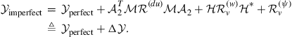
Expression (9.455) reflects the influence of the noises ![]() . Substituting the definition (9.451) into (9.449), and taking the limit as
. Substituting the definition (9.451) into (9.449), and taking the limit as ![]() , we obtain from the latter expression that:
, we obtain from the latter expression that:
![]() (9.456)
(9.456)
which has the same form as (9.284); therefore, we can proceed analogously to obtain:
![]() (9.457)
(9.457)
and
![]() (9.458)
(9.458)
Using (9.455), we see that the network MSD and EMSE deteriorate as follows:
![]() (9.459)
(9.459)
![]() (9.460)
(9.460)
3.09.9.5 Adaptive combination weights
We can repeat the discussion from Sections 3.09.8.2 and 3.09.8.3 to devise one adaptive scheme to adjust the combination coefficients in the noisy exchange case. We illustrate the construction by considering the ATC strategy corresponding to ![]() , so that only weight estimates are exchanged and the update recursions are of the form:
, so that only weight estimates are exchanged and the update recursions are of the form:
![]() (9.461)
(9.461)
![]() (9.462)
(9.462)
where from (9.408):
![]() (9.463)
(9.463)
In this case, the network MSD performance (9.457) becomes
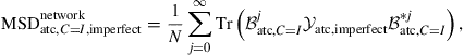 (9.464)
where, since now ![]() and
and ![]() , we have
, we have
![]() (9.465)
(9.465)
![]() (9.466)
(9.466)
![]() (9.467)
(9.467)
![]() (9.468)
(9.468)
![]() (9.469)
(9.469)
![]() (9.470)
(9.470)
![]() (9.471)
(9.471)
![]() (9.472)
(9.472)
To proceed, as was the case with (9.389), we consider the following simplified optimization problem:
 (9.473)
Using (9.466), the trace of ![]() can be expressed in terms of the combination coefficients as follows:
can be expressed in terms of the combination coefficients as follows:
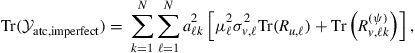 (9.474)
so that problem (9.473) can be decoupled into ![]() separate optimization problems of the form:
separate optimization problems of the form:
 (9.475)
With each node ![]() , we associate the following nonnegative variance products:
, we associate the following nonnegative variance products:
![]() (9.476)
(9.476)
This measure now incorporates information about the exchange noise covariances ![]() . Then, the solution of (9.475) is given by:
. Then, the solution of (9.475) is given by:
 (9.477)
We continue to refer to this combination rule as the relative-variance combination rule [64]; it leads to a left-stochastic matrix ![]() . To evaluate the combination weights (9.477), the nodes need to know the variance products,
. To evaluate the combination weights (9.477), the nodes need to know the variance products, ![]() , of their neighbors. As before, we can motivate one adaptive construction as follows.
, of their neighbors. As before, we can motivate one adaptive construction as follows.
We refer to the ATC recursion (9.461)–(9.463) and use the data model (9.208) to write for node ![]() :
:
![]() (9.478)
(9.478)
so that, in view of our earlier assumptions on the regression data and noise in Sections 3.09.6.1 and 3.09.9.1, we obtain in the limit as ![]() :
:
![]() (9.479)
(9.479)
In a manner similar to what was done before for (9.396), we can evaluate the limit on the right-hand side by using the corresponding steady-state result (9.456). We select the vector ![]() in (9.456) to satisfy:
in (9.456) to satisfy:
![]() (9.480)
(9.480)
Then, from (9.456),
![]() (9.481)
(9.481)
Now recall from expression (9.466) that the entries of ![]() depend on combinations of the squared step-sizes,
depend on combinations of the squared step-sizes, ![]() , and on terms involving
, and on terms involving ![]() . This fact implies that the first term on the right-hand side of (9.479) depends on products of the form
. This fact implies that the first term on the right-hand side of (9.479) depends on products of the form ![]() ; these fourth-order factors can be ignored in comparison to the second-order factor
; these fourth-order factors can be ignored in comparison to the second-order factor ![]() for small step-sizes. Moreover, the same first term on the right-hand side of (9.479) depends on products of the form
for small step-sizes. Moreover, the same first term on the right-hand side of (9.479) depends on products of the form ![]() , which can be ignored in comparison to the last term,
, which can be ignored in comparison to the last term, ![]() in (9.479), which does not appear multiplied by a squared step-size. Therefore, we can approximate:
in (9.479), which does not appear multiplied by a squared step-size. Therefore, we can approximate:
 (9.482)
in terms of the desired variance product, ![]() . Using the following instantaneous approximation at node
. Using the following instantaneous approximation at node ![]() (where
(where ![]() is replaced by
is replaced by ![]() ):
):
![]() (9.483)
(9.483)
we can motivate an algorithm that enables node ![]() to estimate the variance products
to estimate the variance products ![]() . Thus, let
. Thus, let ![]() denote an estimate for
denote an estimate for ![]() that is computed by node
that is computed by node ![]() at time
at time ![]() . Then, one way to evaluate
. Then, one way to evaluate ![]() is through the recursion:
is through the recursion:
![]() (9.484)
(9.484)
where ![]() is a positive coefficient smaller than one. Indeed, it can be verified that
is a positive coefficient smaller than one. Indeed, it can be verified that
![]() (9.485)
(9.485)
so that the estimator ![]() converges on average close to the desired variance product
converges on average close to the desired variance product ![]() . In this way, we can replace the weights (9.477) by the adaptive construction:
. In this way, we can replace the weights (9.477) by the adaptive construction:
 (9.486)
Equations (9.484) and (9.486) provide one adaptive construction for the combination weights ![]() .
.
3.09.10 Extensions and further considerations
Several extensions and variations of diffusion strategies are possible. Among those variations we mention strategies that endow nodes with temporal processing abilities, in addition to their spatial cooperation abilities. We can also apply diffusion strategies to solve recursive least-squares and state-space estimation problems in a distributed manner. In this section, we highlight select contributions in these and related areas.
3.09.10.1 Adaptive diffusion strategies with smoothing mechanisms
In the ATC and CTA adaptive diffusion strategies (9.153) and (9.154), each node in the network shares information locally with its neighbors through a process of spatial cooperation or combination. In this section, we describe briefly an extension that adds a temporal dimension to the processing at the nodes. For example, in the ATC implementation (9.153), rather than have each node ![]() rely solely on current data,
rely solely on current data, ![]() , and on current weight estimates received from the neighbors,
, and on current weight estimates received from the neighbors, ![]() , node
, node ![]() can be allowed to store and process present and past weight estimates, say,
can be allowed to store and process present and past weight estimates, say, ![]() of them as in
of them as in ![]() . In this way, previous weight estimates can be smoothed and used more effectively to help enhance the mean-square-deviation performance especially in the presence of noise over the communication links.
. In this way, previous weight estimates can be smoothed and used more effectively to help enhance the mean-square-deviation performance especially in the presence of noise over the communication links.
To motivate diffusion strategies with smoothing mechanisms, we continue to assume that the random data ![]() satisfy the modeling assumptions of Section 3.09.6.1. The global cost (9.92) continues to be the same but the individual cost functions (9.93) are now replaced by
satisfy the modeling assumptions of Section 3.09.6.1. The global cost (9.92) continues to be the same but the individual cost functions (9.93) are now replaced by
 (9.487)
so that
 (9.488)
where each coefficient ![]() is a nonnegative scalar representing the weight that node
is a nonnegative scalar representing the weight that node ![]() assigns to data from time instant
assigns to data from time instant ![]() . The coefficients
. The coefficients ![]() are assumed to satisfy the normalization condition:
are assumed to satisfy the normalization condition:
 (9.489)
When the random processes ![]() and
and ![]() are jointly wide-sense stationary, as was assumed in Section 3.09.6.1, the optimal solution
are jointly wide-sense stationary, as was assumed in Section 3.09.6.1, the optimal solution ![]() that minimizes (9.488) is still given by the same normal equations (9.40). We can extend the arguments of Sections 3.09.3 and 3.09.4 to (9.488) and arrive at the following version of a diffusion strategy incorporating temporal processing (or smoothing) of the intermediate weight estimates [70,71]:
that minimizes (9.488) is still given by the same normal equations (9.40). We can extend the arguments of Sections 3.09.3 and 3.09.4 to (9.488) and arrive at the following version of a diffusion strategy incorporating temporal processing (or smoothing) of the intermediate weight estimates [70,71]:
![]() (9.490)
(9.490)
 (9.491)
![]() (9.492)
(9.492)
where the nonnegative coefficients ![]() satisfy:
satisfy:
 (9.493)
 (9.494)
 (9.495)
![]() (9.496)
(9.496)
Since only the coefficients ![]() are needed, we alternatively denote them by the simpler notation
are needed, we alternatively denote them by the simpler notation ![]() in the listing in Table 9.8. These are simply chosen as nonnegative coefficients:
in the listing in Table 9.8. These are simply chosen as nonnegative coefficients:
![]() (9.497)
(9.497)
Note that algorithm (9.490)–(9.492) involves three steps: (a) an adaptation step (A) represented by (9.490); (b) a temporal filtering or smoothing step (T) represented by (9.491), and a spatial cooperation step (S) represented by (9.492). These steps are illustrated in Figure 9.15. We use the letters (A, T, S) to label these steps; and we use the sequence of letters (A, T, S) to designate the order of the steps. According to this convention, algorithm (9.490)–(9.492) is referred to as the ATS diffusion strategy since adaptation is followed by temporal processing, which is followed by spatial processing. In total, we can obtain six different combinations of diffusion algorithms by changing the order by which the temporal and spatial combination steps are performed in relation to the adaptation step. The resulting variations are summarized in Table 9.8. When we use only the most recent weight vector in the temporal filtering step (i.e., set ![]() ), which corresponds to the case
), which corresponds to the case ![]() , the algorithms of Table 9.8 reduce to the ATC and CTA diffusion algorithms (9.153) and (9.154). Specifically, the variants TSA, STA, and SAT (where spatial processing S precedes adaptation A) reduce to CTA, while the variants TAS, ATS, and AST (where adaptation A precedes spatial processing S) reduce to ATC.
, the algorithms of Table 9.8 reduce to the ATC and CTA diffusion algorithms (9.153) and (9.154). Specifically, the variants TSA, STA, and SAT (where spatial processing S precedes adaptation A) reduce to CTA, while the variants TAS, ATS, and AST (where adaptation A precedes spatial processing S) reduce to ATC.


Figure 9.15 Illustration of the three steps involved in an ATS diffusion strategy: adaptation, followed by temporal processing or smoothing, followed by spatial processing.
The mean-square performance analysis of the smoothed diffusion strategies can be pursued by extending the arguments of Section 3.09.6. This step is carried out in [70,71] for doubly stochastic combination matrices ![]() when the filtering coefficients
when the filtering coefficients ![]() do not change with
do not change with ![]() . For instance, it is shown in [71] that whether temporal processing is performed before or after adaptation, the strategy that performs adaptation before spatial cooperation is always better. Specifically, the six diffusion variants can be divided into two groups with the respective network MSDs satisfying the following relations:
. For instance, it is shown in [71] that whether temporal processing is performed before or after adaptation, the strategy that performs adaptation before spatial cooperation is always better. Specifically, the six diffusion variants can be divided into two groups with the respective network MSDs satisfying the following relations:
![]() (9.498)
(9.498)
![]() (9.499)
(9.499)
Note that within groups 1 and 2, the order of the A and T operations is the same: in group 1, T precedes A and in group 2, A precedes T. Moreover, within each group, the order of the A and S operations determines performance; the strategy that performs A before S is better. Note further that when ![]() , so that temporal processing is not performed, then TAS reduces to ATC and TSA reduces to CTA. This conclusion is consistent with our earlier result (9.343) that ATC outperforms CTA.
, so that temporal processing is not performed, then TAS reduces to ATC and TSA reduces to CTA. This conclusion is consistent with our earlier result (9.343) that ATC outperforms CTA.
In related work, reference [72] started from the CTA algorithm (9.159) without information exchange and added a useful projection step to it between the combination step and the adaptation step; i.e., the work considered an algorithm with an STA structure (with spatial combination occurring first, followed by a projection step, and then adaptation). The projection step uses the current weight estimate, ![]() , at node
, at node ![]() and projects it onto hyperslabs defined by the current and past raw data. Specifically, the algorithm from [72] has the following form:
and projects it onto hyperslabs defined by the current and past raw data. Specifically, the algorithm from [72] has the following form:
![]() (9.500)
(9.500)
![]() (9.501)
(9.501)
 (9.502)
where the notation ![]() refers to the act of projecting the vector
refers to the act of projecting the vector ![]() onto the hyperslab
onto the hyperslab ![]() that consists of all
that consists of all ![]() vectors
vectors ![]() satisfying (similarly for the projection
satisfying (similarly for the projection ![]() ):
):
![]() (9.503)
(9.503)
![]() (9.504)
(9.504)
where ![]() are positive (tolerance) parameters chosen by the designer to satisfy
are positive (tolerance) parameters chosen by the designer to satisfy ![]() . For generic values
. For generic values ![]() , where
, where ![]() is a scalar and
is a scalar and ![]() is a row vector, the projection operator is described analytically by the following expression [73]:
is a row vector, the projection operator is described analytically by the following expression [73]:
 (9.505)
The projections that appear in (9.501) and (9.502) can be regarded as another example of a temporal processing step. Observe from the middle plot in Figure 9.15 that the temporal step that we are considering in the algorithms listed in Table 9.8 is based on each node ![]() using its current and past weight estimates, such as
using its current and past weight estimates, such as ![]() , rather than only
, rather than only ![]() and current and past raw data
and current and past raw data ![]() . For this reason, the temporal processing steps in Table 9.8 tend to exploit information from across the network more broadly and the resulting mean-square error performance is generally improved relative to (9.500)–(9.502).
. For this reason, the temporal processing steps in Table 9.8 tend to exploit information from across the network more broadly and the resulting mean-square error performance is generally improved relative to (9.500)–(9.502).
3.09.10.2 Diffusion recursive least-squares
Diffusion strategies can also be applied to recursive least-squares problems to enable distributed solutions of least-squares designs [38,39]; see also [74]. Thus, consider again a set of ![]() nodes that are spatially distributed over some domain. The objective of the network is to collectively estimate some unknown column vector of length
nodes that are spatially distributed over some domain. The objective of the network is to collectively estimate some unknown column vector of length ![]() , denoted by
, denoted by ![]() , using a least-squares criterion. At every time instant
, using a least-squares criterion. At every time instant ![]() , each node
, each node ![]() collects a scalar measurement,
collects a scalar measurement, ![]() , which is assumed to be related to the unknown vector
, which is assumed to be related to the unknown vector ![]() via the linear model:
via the linear model:
![]() (9.506)
(9.506)
In the above relation, the vector ![]() denotes a row regression vector of length
denotes a row regression vector of length ![]() , and
, and ![]() denotes measurement noise. A snapshot of the data in the network at time
denotes measurement noise. A snapshot of the data in the network at time ![]() can be captured by collecting the measurements and noise samples,
can be captured by collecting the measurements and noise samples, ![]() from across all nodes into column vectors
from across all nodes into column vectors ![]() and
and ![]() of sizes
of sizes ![]() each, and the regressors
each, and the regressors ![]() into a matrix
into a matrix ![]() of size
of size ![]() :
:
 (9.507)
Likewise, the history of the data across the network up to time ![]() can be collected into vector quantities as follows:
can be collected into vector quantities as follows:
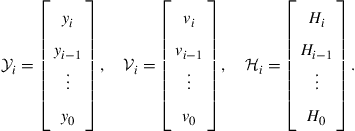 (9.508)
Then, one way to estimate ![]() is by formulating a global least-squares optimization problem of the form:
is by formulating a global least-squares optimization problem of the form:
![]() (9.509)
(9.509)
where ![]() represents a Hermitian regularization matrix and
represents a Hermitian regularization matrix and ![]() represents a Hermitian weighting matrix. Common choices for
represents a Hermitian weighting matrix. Common choices for ![]() and
and ![]() are
are
![]() (9.510)
(9.510)
![]() (9.511)
(9.511)
where ![]() is usually a large number and
is usually a large number and ![]() is a forgetting factor whose value is generally very close to one. In this case, the global cost function (9.509) can be written in the equivalent form:
is a forgetting factor whose value is generally very close to one. In this case, the global cost function (9.509) can be written in the equivalent form:
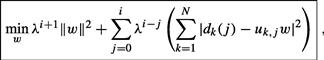 (9.512)
which is an exponentially weighted least-squares problem. We see that, for every time instant ![]() , the squared errors,
, the squared errors, ![]() , are summed across the network and scaled by the exponential weighting factor
, are summed across the network and scaled by the exponential weighting factor ![]() . The index
. The index ![]() denotes current time and the index
denotes current time and the index ![]() denotes a time instant in the past. In this way, data occurring in the remote past are scaled more heavily than data occurring closer to present time.The global solution of (9.509) is given by [5]:
denotes a time instant in the past. In this way, data occurring in the remote past are scaled more heavily than data occurring closer to present time.The global solution of (9.509) is given by [5]:
![]() (9.513)
(9.513)
and the notation ![]() , with a subscript
, with a subscript ![]() , is meant to indicate that the estimate
, is meant to indicate that the estimate ![]() is based on all data collected from across the network up to time
is based on all data collected from across the network up to time ![]() . Therefore, the
. Therefore, the ![]() that is computed via (9.513) amounts to a global construction.
that is computed via (9.513) amounts to a global construction.
In [38,39] a diffusion strategy was developed that allows nodes to approach the global solution ![]() by relying solely on local interactions. Let
by relying solely on local interactions. Let ![]() denote a local estimate for
denote a local estimate for ![]() that is computed by node
that is computed by node ![]() at time
at time ![]() . The diffusion recursive-least-squares (RLS) algorithm takes the following form. For every node
. The diffusion recursive-least-squares (RLS) algorithm takes the following form. For every node ![]() , we start with the initial conditions
, we start with the initial conditions ![]() and
and ![]() where
where ![]() is an
is an ![]() matrix. Then, for every time instant
matrix. Then, for every time instant ![]() , each node
, each node ![]() performs an incremental step followed by a diffusion step as follows:
performs an incremental step followed by a diffusion step as follows:
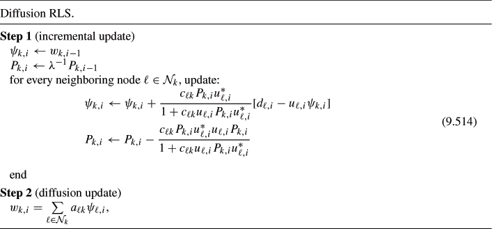
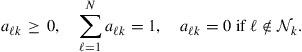
where the symbol ![]() denotes a sequential assignment, and where the scalars
denotes a sequential assignment, and where the scalars ![]() are nonnegative coefficients satisfying:
are nonnegative coefficients satisfying:
 (9.515)
 (9.516)
The above algorithm requires that at every instant ![]() , nodes communicate to their neighbors their measurements
, nodes communicate to their neighbors their measurements ![]() for the incremental update, and the intermediate estimates
for the incremental update, and the intermediate estimates ![]() for the diffusion update. During the incremental update, node
for the diffusion update. During the incremental update, node ![]() cycles through its neighbors and incorporates their data contributions represented by
cycles through its neighbors and incorporates their data contributions represented by ![]() into
into ![]() . Every other node in the network is performing similar steps. At the end of the incremental step, neighboring nodes share their intermediate estimates
. Every other node in the network is performing similar steps. At the end of the incremental step, neighboring nodes share their intermediate estimates ![]() to undergo diffusion. Thus, at the end of both steps, each node
to undergo diffusion. Thus, at the end of both steps, each node ![]() would have updated the quantities
would have updated the quantities ![]() to
to ![]() . The quantities
. The quantities ![]() are matrices of size
are matrices of size ![]() each. Observe that the diffusion RLS implementation (9.514) does not require the nodes to share their matrices
each. Observe that the diffusion RLS implementation (9.514) does not require the nodes to share their matrices ![]() , which would amount to a substantial burden in terms of communications resources since each of these matrices has
, which would amount to a substantial burden in terms of communications resources since each of these matrices has ![]() entries. Only the quantities
entries. Only the quantities ![]() are shared. The mean-square performance and convergence of the diffusion RLS strategy are studied in some detail in [39].
are shared. The mean-square performance and convergence of the diffusion RLS strategy are studied in some detail in [39].
The incremental step of the diffusion RLS strategy (9.514) corresponds to performing a number of ![]() successive least-squares updates starting from the initial conditions
successive least-squares updates starting from the initial conditions ![]() and ending with the values
and ending with the values ![]() that move onto the diffusion update step. It can be verified from the properties of recursive least-squares solutions [4,5] that these variables satisfy the following equations at the end of the incremental stage (step 1):
that move onto the diffusion update step. It can be verified from the properties of recursive least-squares solutions [4,5] that these variables satisfy the following equations at the end of the incremental stage (step 1):
![]() (9.517)
(9.517)
![]() (9.518)
(9.518)
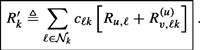
Introduce the auxiliary ![]() variable:
variable:
![]() (9.519)
(9.519)
Then, the above expressions lead to the following alternative form of the diffusion RLS strategy (9.514).

Under some approximations, and for the special choices ![]() and
and ![]() , the diffusion RLS strategy (9.520) can be reduced to a form given in [75] and which is described by the following equations:
, the diffusion RLS strategy (9.520) can be reduced to a form given in [75] and which is described by the following equations:
![]() (9.521)
(9.521)
![]() (9.522)
(9.522)
![]() (9.523)
(9.523)
Algorithm (9.521)–(9.523) is motivated in [75] by using consensus-type arguments. Observe that the algorithm requires the nodes to share the variables ![]() , which corresponds to more communications overburden than required by diffusion RLS; the latter only requires that nodes share
, which corresponds to more communications overburden than required by diffusion RLS; the latter only requires that nodes share ![]() . In order to illustrate how a special case of diffusion RLS (9.520) can be related to this scheme, let us set
. In order to illustrate how a special case of diffusion RLS (9.520) can be related to this scheme, let us set
![]() (9.524)
(9.524)
Then, Eqs. (9.520) give:

Comparing these equations with (9.521)–(9.523), we find that algorithm (9.521)–(9.523) of [75] would relate to the diffusion RLS algorithm (9.520) when the following approximations are justified:
![]() (9.526)
(9.526)
 (9.527)
![]() (9.528)
(9.528)
It was indicated in [39] that the diffusion RLS implementation (9.514) or (9.520) leads to enhanced performance in comparison to the consensus-based update (9.521)–(9.523).
3.09.10.3 Diffusion Kalman filtering
Diffusion strategies can also be applied to the solution of distributed state-space filtering and smoothing problems [35,40,41]. Here, we describe briefly the diffusion version of the Kalman filter; other variants and smoothing filters can be found in [35]. We assume that some system of interest is evolving according to linear state-space dynamics, and that every node in the network collects measurements that are linearly related to the unobserved state vector. The objective is for every node to track the state of the system over time based solely on local observations and on neighborhood interactions.
Thus, consider a network consisting of ![]() nodes observing the state vector,
nodes observing the state vector, ![]() of size
of size ![]() of a linear state-space model. At every time
of a linear state-space model. At every time ![]() , every node
, every node ![]() collects a measurement vector
collects a measurement vector ![]() of size
of size ![]() , which is related to the state vector as follows:
, which is related to the state vector as follows:
![]() (9.529)
(9.529)
![]() (9.530)
(9.530)
The signals ![]() and
and ![]() denote state and measurement noises of sizes
denote state and measurement noises of sizes ![]() and
and ![]() , respectively, and they are assumed to be zero-mean, uncorrelated and white, with covariance matrices denoted by
, respectively, and they are assumed to be zero-mean, uncorrelated and white, with covariance matrices denoted by
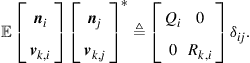 (9.531)
The initial state vector, ![]() is assumed to be zero-mean with covariance matrix
is assumed to be zero-mean with covariance matrix
![]() (9.532)
(9.532)
and is uncorrelated with ![]() and
and ![]() , for all
, for all ![]() and
and ![]() . We further assume that
. We further assume that ![]() . The parameter matrices
. The parameter matrices ![]() are assumed to be known by node
are assumed to be known by node ![]() .
.
Let ![]() denote a local estimator for
denote a local estimator for ![]() that is computed by node
that is computed by node ![]() at time
at time ![]() based solely on local observations and on neighborhood data up to time
based solely on local observations and on neighborhood data up to time ![]() . The following diffusion strategy was proposed in [35,40,41] to approximate predicted and filtered versions of these local estimators in a distributed manner for data satisfying model (9.529)–(9.532). For every node
. The following diffusion strategy was proposed in [35,40,41] to approximate predicted and filtered versions of these local estimators in a distributed manner for data satisfying model (9.529)–(9.532). For every node ![]() , we start with
, we start with ![]() and
and ![]() , where
, where ![]() is an
is an ![]() matrix. At every time instant
matrix. At every time instant ![]() , every node
, every node ![]() performs an incremental step followed by a diffusion step:
performs an incremental step followed by a diffusion step:
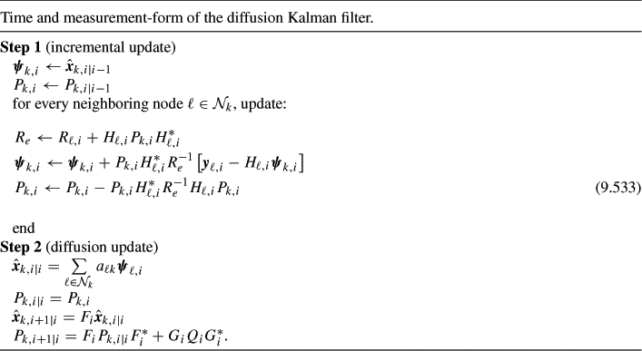
where the symbol ![]() denotes a sequential assignment, and where the scalars
denotes a sequential assignment, and where the scalars ![]() are nonnegative coefficients satisfying:
are nonnegative coefficients satisfying:
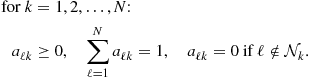 (9.534)
The above algorithm requires that at every instant ![]() , nodes communicate to their neighbors their measurement matrices
, nodes communicate to their neighbors their measurement matrices ![]() , the noise covariance matrices
, the noise covariance matrices ![]() , and the measurements
, and the measurements ![]() for the incremental update, and the intermediate estimators
for the incremental update, and the intermediate estimators ![]() for the diffusion update. During the incremental update, node
for the diffusion update. During the incremental update, node ![]() cycles through its neighbors and incorporates their data contributions represented by
cycles through its neighbors and incorporates their data contributions represented by ![]() into
into ![]() . Every other node in the network is performing similar steps. At the end of the incremental step, neighboring nodes share their updated intermediate estimators
. Every other node in the network is performing similar steps. At the end of the incremental step, neighboring nodes share their updated intermediate estimators ![]() to undergo diffusion. Thus, at the end of both steps, each node
to undergo diffusion. Thus, at the end of both steps, each node ![]() would have updated the quantities
would have updated the quantities ![]() to
to ![]() . The quantities
. The quantities ![]() are
are ![]() matrices. It is important to note that even though the notation
matrices. It is important to note that even though the notation ![]() and
and ![]() has been retained for these variables, as in the standard Kalman filtering notation [5,76], these matrices do not represent any longer the covariances of the state estimation errors,
has been retained for these variables, as in the standard Kalman filtering notation [5,76], these matrices do not represent any longer the covariances of the state estimation errors, ![]() but can be related to them [35].
but can be related to them [35].
An alternative representation of the diffusion Kalman filter may be obtained in information form by further assuming that ![]() for all
for all ![]() and
and ![]() ; a sufficient condition for this fact to hold is to requires the matrices
; a sufficient condition for this fact to hold is to requires the matrices ![]() to be invertible [76]. Thus, consider again data satisfying model (9.529)–(9.532). For every node
to be invertible [76]. Thus, consider again data satisfying model (9.529)–(9.532). For every node ![]() , we start with
, we start with ![]() and
and ![]() . At every time instant
. At every time instant ![]() , every node
, every node ![]() performs an incremental step followed by a diffusion step:
performs an incremental step followed by a diffusion step:

The incremental update in (9.535) is similar to the update used in the distributed Kalman filter derived in [49]. An important difference in the algorithms is in the diffusion step. Reference [49] starts from a continuous-time consensus implementation and discretizes it to arrive at the following update relation:
![]() (9.536)
(9.536)
which, in order to facilitate comparison with (9.535), can be equivalently rewritten as:
![]() (9.537)
(9.537)
where ![]() denotes the degree of node
denotes the degree of node ![]() (i.e., the size of its neighborhood,
(i.e., the size of its neighborhood, ![]() ). In comparison, the diffusion step in (9.535) can be written as:
). In comparison, the diffusion step in (9.535) can be written as:
![]() (9.538)
(9.538)
Observe that the weights used in (9.537) are ![]() for the node’s estimator,
for the node’s estimator, ![]() , and
, and ![]() for all other estimators,
for all other estimators, ![]() , arriving from the neighbors of node
, arriving from the neighbors of node ![]() . In contrast, the diffusion step (9.538) employs a convex combination of the estimators
. In contrast, the diffusion step (9.538) employs a convex combination of the estimators ![]() with generally different weights
with generally different weights ![]() for different neighbors; this choice is motivated by the desire to employ combination coefficients that enhance the fusion of information at node
for different neighbors; this choice is motivated by the desire to employ combination coefficients that enhance the fusion of information at node ![]() , as suggested by the discussion in Appendix D of [35]. It was verified in [35] that the diffusion implementation (9.538) leads to enhanced performance in comparison to the consensus-based update (9.537). Moreover, the weights
, as suggested by the discussion in Appendix D of [35]. It was verified in [35] that the diffusion implementation (9.538) leads to enhanced performance in comparison to the consensus-based update (9.537). Moreover, the weights ![]() in (9.538) can also be adjusted over time in order to further enhance performance, as discussed in [77]. The mean-square performance and convergence of the diffusion Kalman filtering implementations are studied in some detail in [35], along with other diffusion strategies for smoothing problems including fixed-point and fixed-lag smoothing.
in (9.538) can also be adjusted over time in order to further enhance performance, as discussed in [77]. The mean-square performance and convergence of the diffusion Kalman filtering implementations are studied in some detail in [35], along with other diffusion strategies for smoothing problems including fixed-point and fixed-lag smoothing.
3.09.10.4 Diffusion distributed optimization
The ATC and CTA steepest-descent diffusion strategies (9.134) and (9.142) derived earlier in Section 3.09.3 provide distributed mechanisms for the solution of global optimization problems of the form:
 (9.539)
where the individual costs, ![]() , were assumed to be quadratic in
, were assumed to be quadratic in ![]() , namely,
, namely,
![]() (9.540)
(9.540)
for given parameters ![]() . Nevertheless, we remarked in that section that similar diffusion strategies can be applied to more general cases involving individual cost functions,
. Nevertheless, we remarked in that section that similar diffusion strategies can be applied to more general cases involving individual cost functions, ![]() , that are not necessarily quadratic in
, that are not necessarily quadratic in ![]() [1–3]. We restate below, for ease of reference, the general ATC and CTA diffusion strategies (9.139) and (9.146) that can be used for the distributed solution of global optimization problems of the form (9.539) for more general convex functions
[1–3]. We restate below, for ease of reference, the general ATC and CTA diffusion strategies (9.139) and (9.146) that can be used for the distributed solution of global optimization problems of the form (9.539) for more general convex functions ![]() :
:
 (9.541)
and
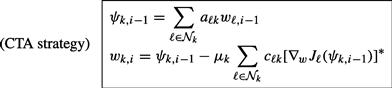 (9.542)
for positive step-sizes ![]() and for nonnegative coefficients
and for nonnegative coefficients ![]() that satisfy:
that satisfy:
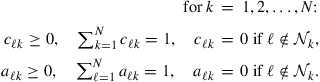 (9.543)
That is, the matrix ![]() is left-stochastic while the matrix
is left-stochastic while the matrix ![]() is right-stochastic:
is right-stochastic:
![]() (9.544)
(9.544)
We can again regard the above ATC and CTA strategies as special cases of the following general diffusion scheme:
![]() (9.545)
(9.545)
![]() (9.546)
(9.546)
![]() (9.547)
(9.547)
where the coefficients ![]() are nonnegative coefficients corresponding to the
are nonnegative coefficients corresponding to the ![]() th entries of combination matrices
th entries of combination matrices ![]() that satisfy:
that satisfy:
![]() (9.548)
(9.548)
The convergence behavior of these diffusion strategies can be examined under both conditions of noiseless updates (when the gradient vectors are available) and noisy updates (when the gradient vectors are subject to gradient noise). The following properties can be proven for the diffusion strategies (9.545)–(9.547) [2]. The statements that follow assume, for convenience of presentation, that all data are real-valued; the conditions would need to be adjusted for complex-valued data.
3.09.10.4.1 Noiseless updates
Let
 (9.549)
denote the global cost function that we wish to minimize. Assume ![]() is strictly convex so that its minimizer
is strictly convex so that its minimizer ![]() is unique. Assume further that each individual cost function
is unique. Assume further that each individual cost function ![]() is convex and has a minimizer at the same
is convex and has a minimizer at the same ![]() . This case is common in practice; situations abound where nodes in a network need to work cooperatively to attain a common objective (such as tracking a target, locating the source of chemical leak, estimating a physical model, or identifying a statistical distribution). The case where the
. This case is common in practice; situations abound where nodes in a network need to work cooperatively to attain a common objective (such as tracking a target, locating the source of chemical leak, estimating a physical model, or identifying a statistical distribution). The case where the ![]() have different individual minimizers is studied in [1,3], where it is shown that the same diffusion strategies of this section are still applicable and nodes would converge instead to a Pareto-optimal solution.
have different individual minimizers is studied in [1,3], where it is shown that the same diffusion strategies of this section are still applicable and nodes would converge instead to a Pareto-optimal solution.
Theorem 9.10.1
Convergence to Optimal Solution: Noise-Free Case
Consider the problem of minimizing the strictly convex global cost (9.549), with the individual cost functions ![]() assumed to be convex with each having a minimizer at the same
assumed to be convex with each having a minimizer at the same ![]() . Assume that all data are real-valued and suppose the Hessian matrices of the individual costs are bounded from below and from above as follows:
. Assume that all data are real-valued and suppose the Hessian matrices of the individual costs are bounded from below and from above as follows:
![]() (9.550)
(9.550)
for some positive constants ![]() . Let
. Let
![]() (9.551)
(9.551)
Assume further that ![]() and that the positive step-sizes are chosen such that:
and that the positive step-sizes are chosen such that:
![]() (9.552)
(9.552)
Then, it holds that ![]() as
as ![]() . That is, the weight estimates generated by (9.545)–(9.547) at all nodes will tend towards the desired global minimizer.
. That is, the weight estimates generated by (9.545)–(9.547) at all nodes will tend towards the desired global minimizer. ![]()
We note that in works on distributed sub-gradient methods (e.g., [36,78]), the norms of the sub-gradients are usually required to be uniformly bounded. Such a requirement is restrictive in the unconstrained optimization of differentiable functions. Condition (9.550) is more relaxed since it allows the gradient vector ![]() to have unbounded norm. This extension is important because requiring bounded gradient norms, as opposed to bounded Hessian matrices, would exclude the possibility of using quadratic costs for the
to have unbounded norm. This extension is important because requiring bounded gradient norms, as opposed to bounded Hessian matrices, would exclude the possibility of using quadratic costs for the ![]() (since the gradient vectors would then be unbounded). And, as we saw in the body of the chapter, quadratic costs play a critical role in adaptation and learning over networks.
(since the gradient vectors would then be unbounded). And, as we saw in the body of the chapter, quadratic costs play a critical role in adaptation and learning over networks.
3.09.10.4.2 Updates with gradient noise
It is often the case that we do not have access to the exact gradient vectors to use in (9.546), but to noisy versions of them, say,
![]() (9.553)
(9.553)
where the random vector variable ![]() refers to gradient noise; its value is generally dependent on the weight-error vector realization,
refers to gradient noise; its value is generally dependent on the weight-error vector realization,
![]() (9.554)
(9.554)
at which the gradient vector is being evaluated. In the presence of gradient noise, the weight estimates at the various nodes become random quantities and we denote them by the boldface notation ![]() . We assume that, conditioned on the past history of the weight estimators at all nodes, namely,
. We assume that, conditioned on the past history of the weight estimators at all nodes, namely,
![]() (9.555)
(9.555)
the gradient noise has zero mean and its variance is upper bounded as follows:
![]() (9.556)
(9.556)
![]() (9.557)
(9.557)
for some ![]() and
and ![]() . Condition (9.557) allows the variance of the gradient noise to be time-variant, so long as it does not grow faster than
. Condition (9.557) allows the variance of the gradient noise to be time-variant, so long as it does not grow faster than ![]() . This condition on the noise is more general than the “uniform-bounded assumption” that appears in [36], which required instead:
. This condition on the noise is more general than the “uniform-bounded assumption” that appears in [36], which required instead:
![]() (9.558)
(9.558)
These two requirements are special cases of (9.557) for ![]() . Furthermore, condition (9.557) is similar to condition (4.3) in [79], which requires the noise variance to satisfy:
. Furthermore, condition (9.557) is similar to condition (4.3) in [79], which requires the noise variance to satisfy:
![]() (9.559)
(9.559)
This requirement can be verified to be a combination of the “relative random noise” and the “absolute random noise” conditions defined in [22]—see [2].
Now, introduce the column vector:
 (9.560)
and let
![]() (9.561)
(9.561)
Let further
![]() (9.562)
(9.562)
where
![]() (9.563)
(9.563)
Then, the following result can be established [2]; it characterizes the network mean-square deviation in steady-state, which is defined as
 (9.564)
Theorem 9.10.2
Mean-Square Stability: Noisy Case
Consider the problem of minimizing the strictly convex global cost (9.549), with the individual cost functions ![]() assumed to be convex with each having a minimizer at the same
assumed to be convex with each having a minimizer at the same ![]() . Assume all data are real-valued and suppose the Hessian matrices of the individual costs are bounded from below and from above as stated in (9.550). Assume further that the diffusion strategy (9.545)–(9.547) employs noisy gradient vectors, where the noise terms are zero mean and satisfy conditions (9.557) and (9.561). We select the positive step-sizes to be sufficiently small and to satisfy:
. Assume all data are real-valued and suppose the Hessian matrices of the individual costs are bounded from below and from above as stated in (9.550). Assume further that the diffusion strategy (9.545)–(9.547) employs noisy gradient vectors, where the noise terms are zero mean and satisfy conditions (9.557) and (9.561). We select the positive step-sizes to be sufficiently small and to satisfy:
 (9.565)
for ![]() . Then, the diffusion strategy (9.545)–(9.547) is mean-square stable and the mean-square-deviation of the network is given by:
. Then, the diffusion strategy (9.545)–(9.547) is mean-square stable and the mean-square-deviation of the network is given by:
![]() (9.566)
(9.566)
where
![]() (9.567)
(9.567)
![]() (9.568)
(9.568)
![]() (9.569)
(9.569)
![]() (9.570)
(9.570)
 (9.571)
![]()
Appendices
A Properties of Kronecker products
For ease of reference, we collect in this appendix some useful properties of Kronecker products. All matrices are assumed to be of compatible dimensions; all inverses are assumed to exist whenever necessary. Let ![]() and
and ![]() be
be ![]() and
and ![]() matrices, respectively. Their Kronecker product is denoted by
matrices, respectively. Their Kronecker product is denoted by ![]() and is defined as the
and is defined as the ![]() matrix whose entries are given by [20]:
matrix whose entries are given by [20]:
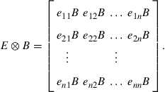 (9.572)
In other words, each entry of ![]() is replaced by a scaled multiple of
is replaced by a scaled multiple of ![]() . Let
. Let ![]() and
and ![]() denote the eigenvalues of
denote the eigenvalues of ![]() and
and ![]() , respectively. Then, the eigenvalues of
, respectively. Then, the eigenvalues of ![]() will consist of all
will consist of all ![]() product combinations
product combinations ![]() . Table 9.9 lists some well-known properties of Kronecker products.
. Table 9.9 lists some well-known properties of Kronecker products.
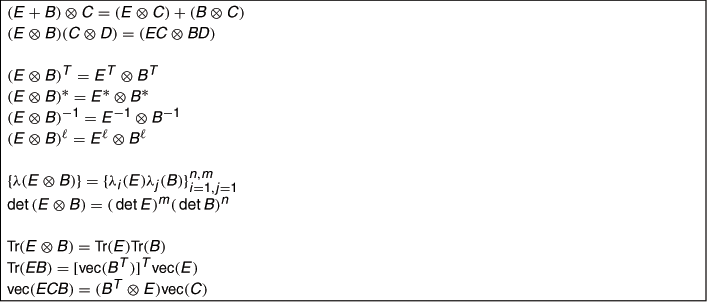
B Graph Laplacian and network connectivity
Consider a network consisting of ![]() nodes and
nodes and ![]() edges connecting the nodes to each other. In the constructions below, we only need to consider the edges that connect distinct nodes to each other; these edges do not contain any self-loops that may exist in the graph and which connect nodes to themselves directly. In other words, when we refer to the
edges connecting the nodes to each other. In the constructions below, we only need to consider the edges that connect distinct nodes to each other; these edges do not contain any self-loops that may exist in the graph and which connect nodes to themselves directly. In other words, when we refer to the ![]() edges of a graph, we are excluding self-loops from this set; but we are still allowing loops of at least length
edges of a graph, we are excluding self-loops from this set; but we are still allowing loops of at least length ![]() (i.e., loops generated by paths covering at least
(i.e., loops generated by paths covering at least ![]() edges).
edges).
The neighborhood of any node ![]() is denoted by
is denoted by ![]() and it consists of all nodes that node
and it consists of all nodes that node ![]() can share information with; these are the nodes that are connected to
can share information with; these are the nodes that are connected to ![]() through edges, in addition to node
through edges, in addition to node ![]() itself. The degree of node
itself. The degree of node ![]() , which we denote by
, which we denote by ![]() , is defined as the positive integer that is equal to the size of its neighborhood:
, is defined as the positive integer that is equal to the size of its neighborhood:
![]() (9.573)
(9.573)
Since ![]() , we always have
, we always have ![]() . We further associate with the network an
. We further associate with the network an ![]() Laplacian matrix, denoted by
Laplacian matrix, denoted by ![]() . The matrix
. The matrix ![]() is symmetric and its entries are defined as follows [60–62]:
is symmetric and its entries are defined as follows [60–62]:
 (9.574)
Note that the term ![]() measures the number of edges that are incident on node
measures the number of edges that are incident on node ![]() , and the locations of the
, and the locations of the ![]() on row
on row ![]() indicate the nodes that are connected to node
indicate the nodes that are connected to node ![]() . We also associate with the graph an
. We also associate with the graph an ![]() incidence matrix, denoted by
incidence matrix, denoted by ![]() . The entries of
. The entries of ![]() are defined as follows. Every column of
are defined as follows. Every column of ![]() represents one edge in the graph. Each edge connects two nodes and its column will display two nonzero entries at the rows corresponding to these nodes: one entry will be
represents one edge in the graph. Each edge connects two nodes and its column will display two nonzero entries at the rows corresponding to these nodes: one entry will be ![]() and the other entry will be
and the other entry will be ![]() . For directed graphs, the choice of which entry is positive or negative can be used to identify the nodes from which edges emanate (source nodes) and the nodes at which edges arrive (sink nodes). Since we are dealing with undirected graphs, we shall simply assign positive values to lower indexed nodes and negative values to higher indexed nodes:
. For directed graphs, the choice of which entry is positive or negative can be used to identify the nodes from which edges emanate (source nodes) and the nodes at which edges arrive (sink nodes). Since we are dealing with undirected graphs, we shall simply assign positive values to lower indexed nodes and negative values to higher indexed nodes:
 (9.575)
Figure 9.16 shows the example of a network with ![]() nodes and
nodes and ![]() edges. Its Laplacian and incidence matrices are also shown and these have sizes
edges. Its Laplacian and incidence matrices are also shown and these have sizes ![]() and
and ![]() , respectively. Consider, for example, column
, respectively. Consider, for example, column ![]() in the incidence matrix. This column corresponds to edge
in the incidence matrix. This column corresponds to edge ![]() , which links nodes
, which links nodes ![]() and
and ![]() . Therefore, at location
. Therefore, at location ![]() we have a
we have a ![]() and at location
and at location ![]() we have
we have ![]() . The other columns of
. The other columns of ![]() are constructed in a similar manner.
are constructed in a similar manner.

Figure 9.16 A network with ![]() nodes and
nodes and ![]() edges. The nodes are marked 1 through 6 and the edges are marked 1 through 8. The corresponding Laplacian and incidence matrices
edges. The nodes are marked 1 through 6 and the edges are marked 1 through 8. The corresponding Laplacian and incidence matrices ![]() and
and ![]() are
are ![]() and
and ![]() .
.
Observe that the Laplacian and incidence matrices of a graph are related as follows:
![]() (9.576)
(9.576)
The Laplacian matrix conveys useful information about the topology of the graph. The following is a classical result from graph theory [60–62,80].
Lemma B.1
Laplacian and Network Connectivity
Let
![]() (9.577)
(9.577)
denote the ordered eigenvalues of ![]() . Then the following properties hold:
. Then the following properties hold:
a. ![]() is symmetric nonnegative-definite so that
is symmetric nonnegative-definite so that ![]() .
.
b. The rows of ![]() add up to zero so that
add up to zero so that ![]() . This means that
. This means that ![]() is a right eigenvector of
is a right eigenvector of ![]() corresponding to the eigenvalue zero.
corresponding to the eigenvalue zero.
c. The smallest eigenvalue is always zero, ![]() . The second smallest eigenvalue,
. The second smallest eigenvalue, ![]() , is called the algebraic connectivity of the graph.
, is called the algebraic connectivity of the graph.
d. The number of times that zero is an eigenvalue of ![]() (i.e., its multiplicity) is equal to the number of connected subgraphs.
(i.e., its multiplicity) is equal to the number of connected subgraphs.
e. The algebraic connectivity of a connected graph is nonzero, i.e., ![]() . In other words, a graph is connected if, and only if, its algebraic connectivity is nonzero.
. In other words, a graph is connected if, and only if, its algebraic connectivity is nonzero.
Proof.
Property (a) follows from the identity ![]() . Property (b) follows from the definition of
. Property (b) follows from the definition of ![]() . Note that for each row of
. Note that for each row of ![]() , the entries on the row add up to zero. Property (c) follows from properties (a) and (b) since
, the entries on the row add up to zero. Property (c) follows from properties (a) and (b) since ![]() implies that zero is an eigenvalue of
implies that zero is an eigenvalue of ![]() . For part (d), assume the network consists of two separate connected subgraphs. Then, the Laplacian matrix would have a block diagonal structure, say, of the form
. For part (d), assume the network consists of two separate connected subgraphs. Then, the Laplacian matrix would have a block diagonal structure, say, of the form ![]() , where
, where ![]() and
and ![]() are the Laplacian matrices of the smaller subgraphs. The smallest eigenvalue of each of these Laplacian matrices would in turn be zero and unique by property (e). More generally, if the graph consists of
are the Laplacian matrices of the smaller subgraphs. The smallest eigenvalue of each of these Laplacian matrices would in turn be zero and unique by property (e). More generally, if the graph consists of ![]() connected subgraphs, then the multiplicity of zero as an eigenvalue of
connected subgraphs, then the multiplicity of zero as an eigenvalue of ![]() would be
would be ![]() . To establish property (e), first observe that if the algebraic connectivity is nonzero then it is obvious that the graph must be connected; otherwise, the Laplacian matrix would be block diagonal and
. To establish property (e), first observe that if the algebraic connectivity is nonzero then it is obvious that the graph must be connected; otherwise, the Laplacian matrix would be block diagonal and ![]() would be zero (a contradiction). For the converse statement, assume the graph is connected and let
would be zero (a contradiction). For the converse statement, assume the graph is connected and let ![]() denote an arbitrary eigenvector of
denote an arbitrary eigenvector of ![]() corresponding to the eigenvalue at zero. Then,
corresponding to the eigenvalue at zero. Then, ![]() , from which we can conclude that all entries of
, from which we can conclude that all entries of ![]() must be equal. Therefore, the algebraic multiplicity of the eigenvalue of
must be equal. Therefore, the algebraic multiplicity of the eigenvalue of ![]() at zero is equal to one and the algebraic connectivity of the graph must be nonzero.
at zero is equal to one and the algebraic connectivity of the graph must be nonzero. ![]()
C Stochastic matrices
Consider ![]() matrices
matrices ![]() with nonnegative entries,
with nonnegative entries, ![]() . The matrix
. The matrix ![]() is said to be right-stochastic if it satisfies
is said to be right-stochastic if it satisfies
![]() (9.578)
(9.578)
in which case each row of ![]() adds up to one. The matrix
adds up to one. The matrix ![]() is said to be left-stochastic if it satisfies
is said to be left-stochastic if it satisfies
![]() (9.579)
(9.579)
in which case each column of ![]() adds up to one. And the matrix is said to be doubly stochastic if both conditions hold so that both its columns and rows add up to one:
adds up to one. And the matrix is said to be doubly stochastic if both conditions hold so that both its columns and rows add up to one:
![]() (9.580)
(9.580)
Stochastic matrices arise frequently in the study of adaptation over networks. This appendix lists some of their properties.
Lemma C.1
Spectral Norm of Stochastic Matrices
Let ![]() be an
be an ![]() right or left or doubly stochastic matrix. Then,
right or left or doubly stochastic matrix. Then, ![]() and, therefore, all eigenvalues of
and, therefore, all eigenvalues of ![]() lie inside the unit disc, i.e.,
lie inside the unit disc, i.e., ![]() .
.
Proof.
We prove the result for right stochastic matrices; a similar argument applies to left or doubly stochastic matrices. Let ![]() be a right-stochastic matrix. Then,
be a right-stochastic matrix. Then, ![]() , so that
, so that ![]() is one of the eigenvalues of
is one of the eigenvalues of ![]() . Moreover, for any matrix
. Moreover, for any matrix ![]() , it holds that
, it holds that ![]() , where
, where ![]() denotes the maximum absolute row sum of its matrix argument. But since all rows of
denotes the maximum absolute row sum of its matrix argument. But since all rows of ![]() add up to one, we have
add up to one, we have ![]() . Therefore,
. Therefore, ![]() . And since we already know that
. And since we already know that ![]() has an eigenvalue at
has an eigenvalue at ![]() , we conclude that
, we conclude that ![]() .
. ![]()
The above result asserts that the spectral radius of a stochastic matrix is unity and that ![]() has an eigenvalue at
has an eigenvalue at ![]() . The result, however, does not rule out the possibility of multiple eigenvalues at
. The result, however, does not rule out the possibility of multiple eigenvalues at ![]() , or even other eigenvalues with magnitude equal to one. Assume, in addition, that the stochastic matrix
, or even other eigenvalues with magnitude equal to one. Assume, in addition, that the stochastic matrix ![]() is regular. This means that there exists an integer power
is regular. This means that there exists an integer power ![]() such that all entries of
such that all entries of ![]() are strictly positive, i.e.,
are strictly positive, i.e.,
![]() (9.581)
(9.581)
Then a result in matrix theory known as the Perron-Frobenius Theorem [20] leads to the following stronger characterization of the eigen-structure of ![]() .
.
Lemma C.2
Spectral Norm of Regular Stochastic Matrices
Let ![]() be an
be an ![]() right stochastic and regular matrix. Then:
right stochastic and regular matrix. Then:
b. All other eigenvalues of ![]() are strictly inside the unit circle (and, hence, have magnitude strictly less than one).
are strictly inside the unit circle (and, hence, have magnitude strictly less than one).
c. The eigenvalue at ![]() is simple, i.e., it has multiplicity one. Moreover, with proper sign scaling, all entries of the corresponding eigenvector are positive. For a right-stochastic
is simple, i.e., it has multiplicity one. Moreover, with proper sign scaling, all entries of the corresponding eigenvector are positive. For a right-stochastic ![]() , this eigenvector is the vector
, this eigenvector is the vector ![]() since
since ![]() .
.
d. All other eigenvectors associated with the other eigenvalues will have at least one negative or complex entry.
Proof.
Part (a) follows from Lemma C.1. Parts (b) and (d) follow from the Perron-Frobenius Theorem when ![]() is regular [20].
is regular [20]. ![]()
Lemma C.3
Useful Properties of Doubly Stochastic Matrices
Let ![]() be an
be an ![]() doubly stochastic matrix. Then the following properties hold:
doubly stochastic matrix. Then the following properties hold:
Proof.
Part (a) follows from Lemma C.1. For part (b), note that ![]() is symmetric and
is symmetric and ![]() Therefore,
Therefore, ![]() is doubly stochastic. Likewise for
is doubly stochastic. Likewise for ![]() . Part (c) follows from part (a) since
. Part (c) follows from part (a) since ![]() and
and ![]() are themselves doubly stochastic matrices. For part (d), note that
are themselves doubly stochastic matrices. For part (d), note that ![]() is symmetric and nonnegative-definite. Therefore, its eigenvalues are real and nonnegative. But since
is symmetric and nonnegative-definite. Therefore, its eigenvalues are real and nonnegative. But since ![]() , we must have
, we must have ![]() . Likewise for the matrix
. Likewise for the matrix ![]() . Part (e) follows from part (d). For part (f), since
. Part (e) follows from part (d). For part (f), since ![]() and its eigenvalues lie within
and its eigenvalues lie within ![]() , the matrix
, the matrix ![]() admits an eigen-decomposition of the form:
admits an eigen-decomposition of the form:
![]()
where ![]() is orthogonal (i.e.,
is orthogonal (i.e., ![]() ) and
) and ![]() is diagonal with entries in the range
is diagonal with entries in the range ![]() . It then follows that
. It then follows that

where step ![]() is because
is because ![]() and, by similarity, the matrix
and, by similarity, the matrix ![]() has the same eigenvalues as
has the same eigenvalues as ![]() . Therefore,
. Therefore, ![]() . This means that the diagonal entries of
. This means that the diagonal entries of ![]() are nonnegative. Multiplying
are nonnegative. Multiplying ![]() by
by ![]() ends up scaling the nonnegative diagonal entries to smaller values so that
ends up scaling the nonnegative diagonal entries to smaller values so that ![]() is justified.
is justified. ![]()
D Block maximum norm
Let ![]() denote an
denote an ![]() block column vector whose individual entries are of size
block column vector whose individual entries are of size ![]() each. Following [23,63,81], the block maximum norm of
each. Following [23,63,81], the block maximum norm of ![]() is denoted by
is denoted by ![]() and is defined as
and is defined as
![]() (9.582)
(9.582)
where ![]() denotes the Euclidean norm of its vector argument. Correspondingly, the induced block maximum norm of an arbitrary
denotes the Euclidean norm of its vector argument. Correspondingly, the induced block maximum norm of an arbitrary ![]() block matrix
block matrix ![]() , whose individual block entries are of size
, whose individual block entries are of size ![]() each, is defined as
each, is defined as
![]() (9.583)
(9.583)
The block maximum norm inherits the unitary invariance property of the Euclidean norm, as the following result indicates [63].
Lemma D.1
Unitary Invariance
Let ![]() be an
be an ![]() block diagonal matrix with
block diagonal matrix with ![]() unitary blocks
unitary blocks ![]() . Then, the following properties hold:
. Then, the following properties hold:
for all block vectors ![]() and block matrices
and block matrices ![]() of appropriate dimensions.
of appropriate dimensions. ![]()
The next result provides useful bounds for the block maximum norm of a block matrix.
Lemma D.2
Useful Bounds
Let ![]() be an arbitrary
be an arbitrary ![]() block matrix with blocks
block matrix with blocks ![]() of size
of size ![]() each. Then, the following results hold:
each. Then, the following results hold:
a. The norms of ![]() and its complex conjugate are related as follows:
and its complex conjugate are related as follows:
![]() (9.584)
(9.584)
b. The norm of ![]() is bounded as follows:
is bounded as follows:
![]() (9.585)
(9.585)
where ![]() denotes the 2-induced norm (or maximum singular value) of its matrix argument.
denotes the 2-induced norm (or maximum singular value) of its matrix argument.
c. If ![]() is Hermitian and nonnegative-definite (
is Hermitian and nonnegative-definite (![]() ), then there exist finite positive constants
), then there exist finite positive constants ![]() and
and ![]() such that
such that
![]() (9.586)
(9.586)
Proof.
Part (a) follows directly from part (b) by noting that

where the equality in the second step is because ![]() ; i.e., complex conjugation does not alter the 2-induced norm of a matrix.
; i.e., complex conjugation does not alter the 2-induced norm of a matrix.
To establish part (b), we consider arbitrary ![]() block vectors
block vectors ![]() with entries
with entries ![]() and where each
and where each ![]() is
is ![]() . Then, note that
. Then, note that
so that
![]()
which establishes the upper bound in (9.585).
To establish the lower bound, we assume without loss of generality that ![]() is attained at
is attained at ![]() and
and ![]() . Let
. Let ![]() denote the largest singular value of
denote the largest singular value of ![]() and let
and let ![]() denote the corresponding
denote the corresponding ![]() right and left singular vectors. That is,
right and left singular vectors. That is,
![]() (9.587)
(9.587)
where ![]() and
and ![]() have unit norms. We now construct an
have unit norms. We now construct an ![]() block vector
block vector ![]() as follows:
as follows:
![]() (9.588)
(9.588)
Then, obviously,
![]() (9.589)
(9.589)
and
![]() (9.590)
(9.590)
It follows that
 (9.591)
Therefore, by the definition of the block maximum norm,
 (9.592)
which establishes the lower bound in (9.585).
To establish part (c), we start by recalling that all norms on finite-dimensional vector spaces are equivalent [20,21]. This means that if ![]() and
and ![]() denote two different matrix norms, then there exist positive constants
denote two different matrix norms, then there exist positive constants ![]() and
and ![]() such that for any matrix
such that for any matrix ![]() ,
,
![]() (9.593)
(9.593)
Now, let ![]() denote the nuclear norm of the square matrix
denote the nuclear norm of the square matrix ![]() . It is defined as the sum of its singular values:
. It is defined as the sum of its singular values:
![]() (9.594)
(9.594)
Since ![]() is Hermitian and nonnegative-definite, its eigenvalues coincide with its singular values and, therefore,
is Hermitian and nonnegative-definite, its eigenvalues coincide with its singular values and, therefore,
![]()
Now applying result (9.593) to the two norms ![]() and
and ![]() we conclude that
we conclude that
![]() (9.595)
(9.595)
as desired. ![]()
The next result relates the block maximum norm of an extended matrix to the ![]() —norm (i.e., maximum absolute row sum) of the originating matrix. Specifically, let
—norm (i.e., maximum absolute row sum) of the originating matrix. Specifically, let ![]() be an
be an ![]() matrix with bounded entries and introduce the block matrix
matrix with bounded entries and introduce the block matrix
![]() (9.596)
(9.596)
The extended matrix ![]() has blocks of size
has blocks of size ![]() each.
each.
Lemma D.3
Relation to Maximum Absolute Row Sum
Let ![]() and
and ![]() be related as in (9.596). Then, the following properties hold:
be related as in (9.596). Then, the following properties hold:
Proof.
The results are obvious for a zero matrix ![]() . So assume
. So assume ![]() is nonzero. Let
is nonzero. Let ![]() denote an arbitrary
denote an arbitrary ![]() block vector whose individual entries
block vector whose individual entries ![]() are vectors of size
are vectors of size ![]() each. Then,
each. Then,
 (9.597)
so that
![]() (9.598)
(9.598)
The argument so far establishes that ![]() . Now, let
. Now, let ![]() denote the row index that corresponds to the maximum absolute row sum of
denote the row index that corresponds to the maximum absolute row sum of ![]() , i.e.,
, i.e.,

We construct an ![]() block vector
block vector ![]() , whose
, whose ![]() entries
entries ![]() are chosen as follows:
are chosen as follows:
![]()
where ![]() is the
is the ![]() basis vector:
basis vector:
![]()
and the sign function is defined as
Then, note that ![]() for any nonzero matrix
for any nonzero matrix ![]() , and
, and
![]()
Moreover,
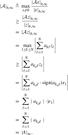 (9.599)
Combining this result with (9.598) we conclude that ![]() , which establishes part (a). Part (b) follows from the statement of part (a) in Lemma D.2.
, which establishes part (a). Part (b) follows from the statement of part (a) in Lemma D.2. ![]()
The next result establishes a useful property for the block maximum norm of right or left stochastic matrices; such matrices arise as combination matrices for distributed processing over networks as in (9.166) and (9.185).
Lemma D.4
Right and Left Stochastic Matrices
Let ![]() be an
be an ![]() right stochastic matrix, i.e., its entries are nonnegative and it satisfies
right stochastic matrix, i.e., its entries are nonnegative and it satisfies ![]() . Let
. Let ![]() be an
be an ![]() left stochastic matrix, i.e., its entries are nonnegative and it satisfies
left stochastic matrix, i.e., its entries are nonnegative and it satisfies ![]() . Introduce the block matrices
. Introduce the block matrices
![]() (9.600)
(9.600)
The matrices ![]() and
and ![]() have blocks of size
have blocks of size ![]() each. It holds that
each. It holds that
![]() (9.601)
(9.601)
Proof.
Since ![]() and
and ![]() are right stochastic matrices, it holds that
are right stochastic matrices, it holds that ![]() and
and ![]() . The desired result then follows from part (a) of Lemma D.3.
. The desired result then follows from part (a) of Lemma D.3. ![]()
The next two results establish useful properties for the block maximum norm of a block diagonal matrix transformed by stochastic matrices; such transformations arise as coefficient matrices that control the evolution of weight error vectors over networks, as in (9.189).
Lemma D.5
Block Diagonal Hermitian Matrices
Consider an ![]() block diagonal Hermitian matrix
block diagonal Hermitian matrix ![]() , where each
, where each ![]() is
is ![]() Hermitian. It holds that
Hermitian. It holds that
![]() (9.602)
(9.602)
where ![]() denotes the spectral radius
denotes the spectral radius ![]() largest eigenvalue magnitude
largest eigenvalue magnitude![]() of its argument. That is, the spectral radius of
of its argument. That is, the spectral radius of ![]() agrees with the block maximum norm of
agrees with the block maximum norm of ![]() , which in turn agrees with the largest spectral radius of its block components.
, which in turn agrees with the largest spectral radius of its block components.
Proof.
We already know that the spectral radius of any matrix ![]() satisfies
satisfies ![]() , for any induced matrix norm [19,20]. Applying this result to
, for any induced matrix norm [19,20]. Applying this result to ![]() we readily get that
we readily get that ![]() . We now establish the reverse inequality, namely,
. We now establish the reverse inequality, namely, ![]() . Thus, pick an arbitrary
. Thus, pick an arbitrary ![]() block vector
block vector ![]() with entries
with entries ![]() , where each
, where each ![]() is
is ![]() . From definition (9.583) we have
. From definition (9.583) we have
 (9.603)
where the notation ![]() denotes the 2-induced norm of
denotes the 2-induced norm of ![]() (i.e., its largest singular value). But since
(i.e., its largest singular value). But since ![]() is assumed to be Hermitian, its 2-induced norm agrees with its spectral radius, which explains the last equality.
is assumed to be Hermitian, its 2-induced norm agrees with its spectral radius, which explains the last equality. ![]()
Lemma D.6
Block Diagonal Matrix Transformed by Left Stochastic Matrices
Consider an ![]() block diagonal Hermitian matrix
block diagonal Hermitian matrix ![]() , where each
, where each ![]() is
is ![]() Hermitian. Let
Hermitian. Let ![]() and
and ![]() be
be ![]() left stochastic matrices, i.e., their entries are nonnegative and they satisfy
left stochastic matrices, i.e., their entries are nonnegative and they satisfy ![]() and
and ![]() Introduce the block matrices
Introduce the block matrices
![]() (9.604)
(9.604)
The matrices ![]() and
and ![]() have blocks of size
have blocks of size ![]() each. Then it holds that
each. Then it holds that
![]() (9.605)
(9.605)
Proof.
Since the spectral radius of any matrix never exceeds any induced norm of the same matrix, we have that
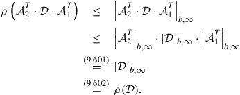 (9.606)
![]()
In view of the result of Lemma D.5, we also conclude from (9.605) that
![]() (9.607)
(9.607)
It is worth noting that there are choices for the matrices ![]() that would result in strict inequality in (9.605). Indeed, consider the special case:
that would result in strict inequality in (9.605). Indeed, consider the special case:

This case corresponds to ![]() and
and ![]() (scalar blocks). Then,
(scalar blocks). Then,
and it is easy to verify that
![]()
The following conclusions follow as corollaries to the statement of Lemma D.6, where by a stable matrix ![]() we mean one whose eigenvalues lie strictly inside the unit circle.
we mean one whose eigenvalues lie strictly inside the unit circle.
Corollary D.1
Stability Properties
Under the same setting of Lemma D.6, the following conclusions hold:
Proof.
Since ![]() is block diagonal, part (a) follows immediately from (9.605) by noting that
is block diagonal, part (a) follows immediately from (9.605) by noting that ![]() whenever
whenever ![]() is stable. [This statement fixes the argument that appeared in Appendix I of [18] and Lemma 2 of [35]. Since the matrix
is stable. [This statement fixes the argument that appeared in Appendix I of [18] and Lemma 2 of [35]. Since the matrix ![]() in Appendix I of [18] and the matrix
in Appendix I of [18] and the matrix ![]() in Lemma 2 of [35] are block diagonal, the
in Lemma 2 of [35] are block diagonal, the ![]() norm should replace the
norm should replace the ![]() norm used there, as in the proof that led to (9.606) and as already done in [63].] For part (b), assume first that
norm used there, as in the proof that led to (9.606) and as already done in [63].] For part (b), assume first that ![]() is stable, then
is stable, then ![]() will also be stable by part (a) for any left-stochastic matrices
will also be stable by part (a) for any left-stochastic matrices ![]() and
and ![]() . To prove the converse, assume that
. To prove the converse, assume that ![]() is stable for any choice of left stochastic matrices
is stable for any choice of left stochastic matrices ![]() and
and ![]() . Then,
. Then, ![]() is stable for the particular choice
is stable for the particular choice ![]() and it follows that
and it follows that ![]() must be stable.
must be stable. ![]()
E Comparison with consensus strategies
Consider a connected network consisting of ![]() nodes. Each node has a state or measurement value
nodes. Each node has a state or measurement value ![]() , possibly a vector of size
, possibly a vector of size ![]() . All nodes in the network are interested in evaluating the average value of their states, which we denote by
. All nodes in the network are interested in evaluating the average value of their states, which we denote by
 (9.608)
A centralized solution to this problem would require each node to transmit its measurement ![]() to a fusion center. The central processor would then compute
to a fusion center. The central processor would then compute ![]() using (9.608) and transmit it back to all nodes. This centralized mode of operation suffers from at least two limitations. First, it requires communications and power resources to transmit the data back and forth between the nodes and the central processor; this problem is compounded if the fusion center is stationed at a remote location. Second, the architecture has a critical point of failure represented by the central processor; if it fails, then operations would need to be halted.
using (9.608) and transmit it back to all nodes. This centralized mode of operation suffers from at least two limitations. First, it requires communications and power resources to transmit the data back and forth between the nodes and the central processor; this problem is compounded if the fusion center is stationed at a remote location. Second, the architecture has a critical point of failure represented by the central processor; if it fails, then operations would need to be halted.
E.1 Consensus recursion
The consensus strategy provides an elegant distributed solution to the same problem, whereby nodes interact locally with their neighbors and are able to converge to ![]() through these interactions. Thus, consider an arbitrary node
through these interactions. Thus, consider an arbitrary node ![]() and assign nonnegative weights
and assign nonnegative weights ![]() to the edges linking
to the edges linking ![]() to its neighbors
to its neighbors ![]() . For each node
. For each node ![]() , the weights
, the weights ![]() are assumed to add up to one so that
are assumed to add up to one so that
 (9.609)
The resulting combination matrix is denoted by ![]() and its
and its ![]() th column consists of the entries
th column consists of the entries ![]() . In view of (9.609), the combination matrix
. In view of (9.609), the combination matrix ![]() is seen to satisfy
is seen to satisfy ![]() . That is,
. That is, ![]() is left-stochastic. The consensus strategy can be described as follows. Each node
is left-stochastic. The consensus strategy can be described as follows. Each node ![]() operates repeatedly on the data from its neighbors and updates its state iteratively according to the rule:
operates repeatedly on the data from its neighbors and updates its state iteratively according to the rule:
![]() (9.610)
(9.610)
where ![]() denotes the state of node
denotes the state of node ![]() at iteration
at iteration ![]() , and
, and ![]() denotes the updated state of node
denotes the updated state of node ![]() after iteration
after iteration ![]() . The initial conditions are
. The initial conditions are
![]() (9.611)
(9.611)
If we collect the states of all nodes at iteration ![]() into a column vector, say,
into a column vector, say,
![]() (9.612)
(9.612)
Then, the consensus iteration (9.610) can be equivalently rewritten in vector form as follows:
![]() (9.613)
(9.613)
where
![]() (9.614)
(9.614)
The initial condition is
![]() (9.615)
(9.615)
E.2 Error recursion
Note that we can express the average value, ![]() , from (9.608) in the form
, from (9.608) in the form
![]() (9.616)
(9.616)
where ![]() is the vector of size
is the vector of size ![]() and whose entries are all equal to one. Let
and whose entries are all equal to one. Let
![]() (9.617)
(9.617)
denote the weight error vector for node ![]() at iteration
at iteration ![]() ; it measures how far the iterated state is from the desired average value
; it measures how far the iterated state is from the desired average value ![]() . We collect all error vectors across the network into an
. We collect all error vectors across the network into an ![]() block column vector whose entries are of size
block column vector whose entries are of size ![]() each:
each:
 (9.618)
Then,
![]() (9.619)
(9.619)
E.2.1 Convergence conditions
The following result is a classical result on consensus strategies [43–45]. It provides conditions under which the state of all nodes will converge to the desired average, ![]() , so that
, so that ![]() will tend to zero.
will tend to zero.
Theorem E.1
Convergence to Consensus
For any initial states ![]() , the successive iterates
, the successive iterates ![]() generated by the consensus iteration (9.610) converge to the network average value
generated by the consensus iteration (9.610) converge to the network average value ![]() as
as ![]() if, and only if, the following three conditions are met:
if, and only if, the following three conditions are met:
![]() (9.620)
(9.620)
![]() (9.621)
(9.621)
![]() (9.622)
(9.622)
That is, the combination matrix ![]() needs to be doubly stochastic, and the matrix
needs to be doubly stochastic, and the matrix ![]() needs to be stable.
needs to be stable.
Proof.
[Proof (Sufficiency)]Assume first that the three conditions stated in the theorem hold. Since ![]() is doubly stochastic, then so is any power of
is doubly stochastic, then so is any power of ![]() , say,
, say, ![]() for any
for any ![]() , so that
, so that
![]() (9.623)
(9.623)
Using this fact, it is straightforward to verify by induction the validity of the following equality:
![]() (9.624)
(9.624)
Likewise, using the Kronecker product identities
![]() (9.625)
(9.625)
![]() (9.626)
(9.626)
![]() (9.627)
(9.627)
for matrices ![]() of compatible dimensions, we observe that
of compatible dimensions, we observe that
 (9.628)
Iterating (9.613) we find that
![]() (9.629)
(9.629)
and, hence, from (9.616) and (9.619),
 (9.630)
Now recall that, for two arbitrary matrices ![]() and
and ![]() of compatible dimensions, the eigenvalues of the Kronecker product
of compatible dimensions, the eigenvalues of the Kronecker product ![]() is formed of all product combinations
is formed of all product combinations ![]() of the eigenvalues of
of the eigenvalues of ![]() and
and ![]() [19]. We conclude from this property, and from the fact that
[19]. We conclude from this property, and from the fact that ![]() is stable, that the coefficient matrix
is stable, that the coefficient matrix
![]()
is also stable. Therefore,
![]() (9.631)
(9.631)
(Necessity). In order for ![]() in (9.629) to converge to
in (9.629) to converge to ![]() , for any initial state
, for any initial state ![]() , it must hold that
, it must hold that
![]() (9.632)
(9.632)
for any ![]() . This implies that we must have
. This implies that we must have
![]() (9.633)
(9.633)
or, equivalently,
![]() (9.634)
(9.634)
This in turn implies that we must have
![]() (9.635)
(9.635)
But since
![]() (9.636)
(9.636)
we conclude from (9.634) and (9.635) that it must hold that
![]() (9.637)
(9.637)
That is,
![]() (9.638)
(9.638)
from which we conclude that we must have ![]() . Similarly, we can show that
. Similarly, we can show that ![]() by studying the limit of
by studying the limit of ![]() . Therefore,
. Therefore, ![]() must be a doubly stochastic matrix. Now using the fact that
must be a doubly stochastic matrix. Now using the fact that ![]() is doubly stochastic, we know that (9.624) holds. It follows that in order for condition (9.634) to be satisfied, we must have
is doubly stochastic, we know that (9.624) holds. It follows that in order for condition (9.634) to be satisfied, we must have
![]() (9.639)
(9.639)
![]()
E.2.2 Rate of convergence
From (9.630) we conclude that the rate of convergence of the error vectors ![]() to zero is determined by the spectrum of the matrix
to zero is determined by the spectrum of the matrix
![]() (9.640)
(9.640)
Now since ![]() is a doubly stochastic matrix, we know that it has an eigenvalue at
is a doubly stochastic matrix, we know that it has an eigenvalue at ![]() . Let us denote the eigenvalues of
. Let us denote the eigenvalues of ![]() by
by ![]() and let us order them in terms of their magnitudes as follows:
and let us order them in terms of their magnitudes as follows:
![]() (9.641)
(9.641)
where ![]() . Then, the eigenvalues of the coefficient matrix
. Then, the eigenvalues of the coefficient matrix ![]() are equal to
are equal to
![]() (9.642)
(9.642)
It follows that the magnitude of ![]() becomes the spectral radius of
becomes the spectral radius of ![]() . Then condition (9.639) ensures that
. Then condition (9.639) ensures that ![]() . We therefore arrive at the following conclusion.
. We therefore arrive at the following conclusion.
Corollary E.1
Rate of Convergence of Consensus
Under conditions (9.620)–(9.622), the rate of convergence of the successive iterates ![]() towards the network average
towards the network average ![]() in the consensus strategy (9.610) is determined by the second largest eigenvalue magnitude of
in the consensus strategy (9.610) is determined by the second largest eigenvalue magnitude of ![]() , i.e., by
, i.e., by ![]() as defined in (9.641).
as defined in (9.641). ![]()
It is worth noting that doubly stochastic matrices ![]() that are also regular satisfy conditions (9.620)–(9.622). This is because, as we already know from Lemma C.2, the eigenvalues of such matrices satisfy
that are also regular satisfy conditions (9.620)–(9.622). This is because, as we already know from Lemma C.2, the eigenvalues of such matrices satisfy ![]() , for
, for ![]() , so that condition (9.622) is automatically satisfied.
, so that condition (9.622) is automatically satisfied.
Corollary E.2
Convergence for Regular Combination Matrices
Any doubly-stochastic and regular matrix ![]() satisfies the three conditions (9.620)–(9.622) and, therefore, ensures the convergence of the consensus iterates
satisfies the three conditions (9.620)–(9.622) and, therefore, ensures the convergence of the consensus iterates ![]() generated by (9.610) towards
generated by (9.610) towards ![]() as
as ![]() .
. ![]()
A regular combination matrix ![]() would result when the two conditions listed below are satisfied by the graph connecting the nodes over which the consensus iteration is applied.
would result when the two conditions listed below are satisfied by the graph connecting the nodes over which the consensus iteration is applied.
Corollary E.3
Sufficient Condition for Regularity
Assume the combination matrix ![]() is doubly stochastic and that the graph over which the consensus iteration (9.610) is applied satisfies the following two conditions:
is doubly stochastic and that the graph over which the consensus iteration (9.610) is applied satisfies the following two conditions:
a. The graph is connected. This means that there exists a path connecting any two arbitrary nodes in the network. In terms of the Laplacian matrix that is associated with the graph (see Lemma B.1), this means that the second smallest eigenvalue of the Laplacian is nonzero.
b. ![]() if, and only if,
if, and only if, ![]() . That is, the combination weights are strictly positive between any two neighbors, including
. That is, the combination weights are strictly positive between any two neighbors, including ![]() .
.
Then, the corresponding matrix ![]() will be regular and, therefore, the consensus iterates
will be regular and, therefore, the consensus iterates ![]() generated by (9.610) will converge towards
generated by (9.610) will converge towards ![]() as
as ![]() .
.
Proof.
We first establish that conditions (a) and (b) imply that ![]() is a regular matrix, namely, that there should exist an integer
is a regular matrix, namely, that there should exist an integer ![]() such that
such that
![]() (9.643)
(9.643)
for all ![]() . To begin with, by the rules of matrix multiplication, the
. To begin with, by the rules of matrix multiplication, the ![]() entry of the
entry of the ![]() th power of
th power of ![]() is given by
is given by
 (9.644)
The summand in (9.644) is nonzero if, and only if, there is some sequence of indices ![]() that forms a path from node
that forms a path from node ![]() to node
to node ![]() . Since the network is assumed to be connected, there exists a minimum (and finite) integer value
. Since the network is assumed to be connected, there exists a minimum (and finite) integer value ![]() such that a path exists from node
such that a path exists from node ![]() to node
to node ![]() using
using ![]() edges and that
edges and that
![]()
In addition, by induction, if ![]() , then
, then

Let
![]()
Then, property (9.643) holds for all ![]() . And we conclude from (9.581) that
. And we conclude from (9.581) that ![]() is a regular matrix. It then follows from Corollary E.2 that the consensus iterates
is a regular matrix. It then follows from Corollary E.2 that the consensus iterates ![]() converge to the average network value
converge to the average network value ![]() .
. ![]()
E.2.3 Comparison with diffusion strategies
Observe that in comparison to diffusion strategies, such as the ATC strategy (9.153), the consensus iteration (9.610) employs the same quantities ![]() on both sides of the iteration. In other words, the consensus construction keeps iterating on the same set of vectors until they converge to the average value
on both sides of the iteration. In other words, the consensus construction keeps iterating on the same set of vectors until they converge to the average value ![]() . Moreover, the index
. Moreover, the index ![]() in the consensus algorithm is an iteration index. In contrast, diffusion strategies employ different quantities on both sides of the combination step in (9.153), namely,
in the consensus algorithm is an iteration index. In contrast, diffusion strategies employ different quantities on both sides of the combination step in (9.153), namely, ![]() and
and ![]() ; the latter variables have been processed through an information exchange step and are updated (or filtered) versions of the
; the latter variables have been processed through an information exchange step and are updated (or filtered) versions of the ![]() . In addition, each step of the diffusion strategy (9.153) can incorporate new data,
. In addition, each step of the diffusion strategy (9.153) can incorporate new data, ![]() , that are collected by the nodes at every time instant. Moreover, the index
, that are collected by the nodes at every time instant. Moreover, the index ![]() in the diffusion implementation is a time index (and not an iteration index); this is because diffusion strategies are inherently adaptive and perform online learning. Data keeps streaming in and diffusion incorporates the new data into the update equations at every time instant. As a result, diffusion strategies are able to respond to data in an adaptive manner, and they are also able to solve general optimization problems: the vector
in the diffusion implementation is a time index (and not an iteration index); this is because diffusion strategies are inherently adaptive and perform online learning. Data keeps streaming in and diffusion incorporates the new data into the update equations at every time instant. As a result, diffusion strategies are able to respond to data in an adaptive manner, and they are also able to solve general optimization problems: the vector ![]() in adaptive diffusion iterations is the minimizer of a global cost function (cf. (9.92)), while the vector
in adaptive diffusion iterations is the minimizer of a global cost function (cf. (9.92)), while the vector ![]() in consensus iterations is the average value of the initial states of the nodes (cf. (9.608)).
in consensus iterations is the average value of the initial states of the nodes (cf. (9.608)).
It turns out that diffusion strategies influence the evolution of the network dynamics in an interesting and advantageous manner in comparison to consensus strategies. We illustrate this point by means of an example. Consider initially the ATC strategy (9.158) without information exchange, whose update equation we repeat below for ease of reference:
![]() (9.645)
(9.645)
![]() (9.646)
(9.646)
These recursions were derived in the body of the chapter as an effective distributed solution for optimizing (9.92) and (9.93). Note that they involve two steps, where the weight estimator ![]() is first updated to the intermediate estimator
is first updated to the intermediate estimator ![]() , before the intermediate estimators from across the neighborhood are combined to obtain
, before the intermediate estimators from across the neighborhood are combined to obtain ![]() . Both steps of ATC diffusion (9.645) and (9.646) can be combined into a single update as follows:
. Both steps of ATC diffusion (9.645) and (9.646) can be combined into a single update as follows:
![]() (9.647)
(9.647)
Likewise, consider the CTA strategy (9.159) without information exchange, whose update equation we also repeat below:
![]() (9.648)
(9.648)
![]() (9.649)
(9.649)
Again, the CTA strategy involves two steps: the weight estimators ![]() from the neighborhood of node
from the neighborhood of node ![]() are first combined to yield the intermediate estimator
are first combined to yield the intermediate estimator ![]() , which is subsequently updated to
, which is subsequently updated to ![]() . Both steps of CTA diffusion can also be combined into a single update as follows:
. Both steps of CTA diffusion can also be combined into a single update as follows:
 (9.650)
Now, motivated by the consensus iteration (9.610), and based on a procedure for distributed optimization suggested in [23] (see expression (7.1) in that reference), some works in the literature (e.g., [46,53,82–88]) considered distributed strategies that correspond to the following form for the optimization problem under consideration (see, e.g., expression (1.20) in [53] and expression (9) in [87]):
![]() (9.651)
(9.651)
This strategy can be derived by following the same argument we employed earlier in Sections 3.09.3.2 and 3.09.4 to arrive at the diffusion strategies, namely, we replace ![]() in (9.127) by
in (9.127) by ![]() and then apply the instantaneous approximations (9.150). Note that the same variable
and then apply the instantaneous approximations (9.150). Note that the same variable ![]() appears on both sides of the equality in (9.651). Thus, compared with the ATC diffusion strategy (9.647), the update from
appears on both sides of the equality in (9.651). Thus, compared with the ATC diffusion strategy (9.647), the update from ![]() to
to ![]() in the consensus implementation (9.651) is only influenced by data
in the consensus implementation (9.651) is only influenced by data ![]() from node
from node ![]() . In contrast, the ATC diffusion structure (9.645), (9.646) helps incorporate the influence of the data
. In contrast, the ATC diffusion structure (9.645), (9.646) helps incorporate the influence of the data ![]() from across the neighborhood of node
from across the neighborhood of node ![]() into the update of
into the update of ![]() , since these data are reflected in the intermediate estimators
, since these data are reflected in the intermediate estimators ![]() . Likewise, the contrast with the CTA diffusion strategy (9.650) is clear, where the right-most term in (9.650) relies on a combination of all estimators from across the neighborhood of node
. Likewise, the contrast with the CTA diffusion strategy (9.650) is clear, where the right-most term in (9.650) relies on a combination of all estimators from across the neighborhood of node ![]() , and not only on
, and not only on ![]() as in the consensus strategy (9.651). These facts have desirable implications on the evolution of the weight-error vectors across diffusion networks. Some simple algebra, similar to what we did in Section 3.09.6, will show that the mean of the extended error vector for the consensus strategy (9.651) evolves according to the recursion:
as in the consensus strategy (9.651). These facts have desirable implications on the evolution of the weight-error vectors across diffusion networks. Some simple algebra, similar to what we did in Section 3.09.6, will show that the mean of the extended error vector for the consensus strategy (9.651) evolves according to the recursion:
![]() (9.652)
(9.652)
where ![]() is the block diagonal covariance matrix defined by (9.184) and
is the block diagonal covariance matrix defined by (9.184) and ![]() is the aggregate error vector defined by (9.230). We can compare the above mean error dynamics with the ones that correspond to the ATC and CTA diffusion strategies (9.645), (9.646) and (9.648)–(9.650); their error dynamics follow as special cases from (9.248) by setting
is the aggregate error vector defined by (9.230). We can compare the above mean error dynamics with the ones that correspond to the ATC and CTA diffusion strategies (9.645), (9.646) and (9.648)–(9.650); their error dynamics follow as special cases from (9.248) by setting ![]() and
and ![]() for ATC and
for ATC and ![]() and
and ![]() for CTA:
for CTA:
![]() (9.653)
(9.653)
and
![]() (9.654)
(9.654)
We observe that the coefficient matrices that control the evolution of ![]() are different in all three cases. In particular,
are different in all three cases. In particular,
![]() (9.655)
(9.655)
![]() (9.656)
(9.656)
![]() (9.657)
(9.657)
It follows that the mean stability of the consensus network is sensitive to the choice of the combination matrix ![]() . This is not the case for the diffusion strategies. This is because from property (9.605) established in Appendix D, we know that the matrices
. This is not the case for the diffusion strategies. This is because from property (9.605) established in Appendix D, we know that the matrices ![]() and
and ![]() are stable if
are stable if ![]() is stable. Therefore, we can select the step-sizes to satisfy
is stable. Therefore, we can select the step-sizes to satisfy ![]() for the ATC or CTA diffusion strategies and ensure their mean stability regardless of the combination matrix
for the ATC or CTA diffusion strategies and ensure their mean stability regardless of the combination matrix ![]() . This also means that the diffusion networks will be mean stable whenever the individual nodes are mean stable, regardless of the topology defined by
. This also means that the diffusion networks will be mean stable whenever the individual nodes are mean stable, regardless of the topology defined by ![]() . In contrast, for consensus networks, the network can exhibit unstable mean behavior even if all its individual nodes are stable in the mean. For further details and other results on the mean-square performance of diffusion networks in relation to consensus networks, the reader is referred to [89,90].
. In contrast, for consensus networks, the network can exhibit unstable mean behavior even if all its individual nodes are stable in the mean. For further details and other results on the mean-square performance of diffusion networks in relation to consensus networks, the reader is referred to [89,90].
References
1. Chen J, Sayed AH. On the limiting behavior of distributed optimization strategies. In: Proc 50th Annual Allerton Conference on Communication, Control, and Computing. IL: Allerton; October 2012;1535–1542.
2. Chen J, Sayed AH. Diffusion adaptation strategies for distributed optimization and learning over networks. IEEE Trans Signal Process. 2012;60(8):4289–4305.
3. Chen J, Sayed AH. Distributed Pareto optimization via diffusion strategies. IEEE J Sel Top Signal Process. 2013;7(2):205–220.
4. Sayed AH. Fundamentals of Adaptive Filtering. NJ: Wiley; 2003.
5. Sayed AH. Adaptive Filters. NJ: Wiley; 2008.
6. Haykin S. Adaptive Filter Theory. NJ: Prentice Hall; 2002.
7. Widrow B, Stearns SD. Adaptive Signal Processing. NJ: Prentice Hall; 1985.
8. Tu S-Y, Sayed AH. Mobile adaptive networks. IEEE J Sel Top Signal Process. 2011;5(4):649–664.
9. Cattivelli F, Sayed AH. Modeling bird flight formations using diffusion adaptation. IEEE Trans Signal Process. 2011;59(5):2038–2051.
10. Li J, Sayed AH. Modeling bee swarming behavior through diffusion adaptation with asymmetric information sharing. EURASIP J Adv Signal Process. 2012;2012. doi 10.1186/1687-6180-2012-18.
11. Chen J, Sayed AH. Bio-inspired cooperative optimization with application to bacteria motility. In: Proceedings of the ICASSP, Prague, Czech Republic. May 2011;5788–5791.
12. Sayed AH, Sayed FA. Diffusion adaptation over networks of particles subject to Brownian fluctuations. In: Proceedings of the Asilomar Conference on Signals, Systems, and Computers, Pacific Grove, CA. November 2011;685–690.
13. Mitola J, Maguire GQ. Cognitive radio: making software radios more personal. IEEE Personal Commun. 1999;6:13–18.
14. Haykin S. Cognitive radio: brain-empowered wireless communications. IEEE J Sel Areas Commun. 2005;23(2):201–220.
15. Quan Z, Zhang W, Shellhammer SJ, Sayed AH. Optimal spectral feature detection for spectrum sensing at very low SNR. IEEE Trans Commun. 2011;59(1):201–212.
16. Zou Q, Zheng S, Sayed AH. Cooperative sensing via sequential detection. IEEE Trans Signal Process. 2010;58(12):6266–6283.
17. Di Lorenzo P, Barbarossa S, Sayed AH. Bio-inspired swarming for dynamic radio access based on diffusion adaptation. In: Proceedings of the EUSIPCO, Barcelona, Spain. August 2011;402–406.
18. Cattivelli FS, Sayed AH. Diffusion LMS strategies for distributed estimation. IEEE Trans Signal Process. 2010;58(3):1035–1048.
19. Golub GH, Van Loan CF. Matrix Computations. third ed. Baltimore: The John Hopkins University Press; 1996.
20. Horn RA, Johnson CR. Matrix Analysis. Cambridge University Press 2003.
21. Kreyszig E. Introductory Functional Analysis with Applications. NY: Wiley; 1989.
22. Poljak B. Introduction to Optimization. NY: Optimization Software; 1987.
23. Bertsekas DP, Tsitsiklis JN. Parallel and Distributed Computation: Numerical Methods. first ed. Singapore: Athena Scientific; 1997.
24. Bertsekas DP. A new class of incremental gradient methods for least squares problems. SIAM J Optim. 1997;7(4):913–926.
25. Nedic A, Bertsekas DP. Incremental subgradient methods for nondifferentiable optimization. SIAM J Optim. 2001;12(1):109–138.
26. Rabbat MG, Nowak RD. Quantized incremental algorithms for distributed optimization. IEEE J Sel Areas Commun. 2005;23(4):798–808.
27. Lopes CG, Sayed AH. Incremental adaptive strategies over distributed networks. IEEE Trans Signal Process. 2007;55(8):4064–4077.
28. Cattivelli FS, Sayed AH. Diffusion LMS algorithms with information exchange. In: Proceedings of the Asilomar Conference on Signals, Systems and Computers, Pacific Grove, CA. November 2008;251–255.
29. Lopes CG, Sayed AH. Distributed processing over adaptive networks. In: Proceedings of the Adaptive Sensor Array Processing Workshop. MA: MIT Lincoln Laboratory; June 2006;1–5.
30. Sayed AH, Lopes CG. Adaptive processing over distributed networks. IEICE Trans Fund Electron Commun Comput Sci. 2007;E90-A(8):1504–1510.
31. Lopes CG, Sayed AH. Diffusion least-mean-squares over adaptive networks. Proceedings of the IEEE ICASSP, Honolulu, Hawaii. 2007;3:917–920.
32. Lopes CG, Sayed AH. Steady-state performance of adaptive diffusion least-mean squares. In: Proceedings of the IEEE Workshop on Statistical Signal Processing (SSP), Madison, WI. August 2007;136–140.
33. Lopes CG, Sayed AH. Diffusion least-mean squares over adaptive networks: Formulation and performance analysis. IEEE Trans Signal Process. 2008;56(7):3122–3136.
34. Sayed AH, Cattivelli F. Distributed adaptive learning mechanisms. In: Haykin S, Ray Liu KJ, eds. Handbook on Array Processing and Sensor Networks. NJ: Wiley; 2009;695–722.
35. Cattivelli F, Sayed AH. Diffusion strategies for distributed Kalman filtering and smoothing. IEEE Trans Autom Control. 2010;55(9):2069–2084.
36. Ram SS, Nedic A, Veeravalli VV. Distributed stochastic subgradient projection algorithms for convex optimization. J Optim Theory Appl. 2010;147(3):516–545.
37. Bianchi P, Fort G, Hachem W, Jakubowicz J. Convergence of a distributed parameter estimator for sensor networks with local averaging of the estimates. In: Proceedings of the IEEE ICASSP, Prague, Czech. May 2011;3764–3767.
38. Cattivelli FS, Lopes CG, Sayed AH. A diffusion RLS scheme for distributed estimation over adaptive networks. In: Proceedings of the IEEE Workshop on Signal Processing Advances Wireless Communications (SPAWC), Helsinki, Finland. June 2007;1–5.
39. Cattivelli FS, Lopes CG, Sayed AH. Diffusion recursive least-squares for distributed estimation over adaptive networks. IEEE Trans Signal Process. 2008;56(5):1865–1877.
40. Cattivelli FS, Lopes CG, Sayed AH. Diffusion strategies for distributed Kalman filtering: formulation and performance analysis. In: Proceedings of the IAPR Workshop on Cognitive Information Process (CIP), Santorini, Greece. June 2008;36–41.
41. Cattivelli FS, Sayed AH. Diffusion mechanisms for fixed-point distributed Kalman smoothing. In: Proceedings of the EUSIPCO, Lausanne, Switzerland. August 2008;1–4.
42. Stankovic SS, Stankovic MS, Stipanovic DS. Decentralized parameter estimation by consensus based stochastic approximation. IEEE Trans Autom Control. 2011;56(3):531–543.
43. DeGroot MH. Reaching a consensus. J Am Stat Assoc. 1974;69(345):118–121.
44. Berger RL. A necessary and sufficient condition for reaching a consensus using DeGroot’s method. J Am Stat Assoc. 1981;76(374):415–418.
45. Tsitsiklis J, Athans M. Convergence and asymptotic agreement in distributed decision problems. IEEE Trans Autom Control. 1984;29(1):42–50.
46. Jadbabaie A, Lin J, Morse AS. Coordination of groups of mobile autonomous agents using nearest neighbor rules. IEEE Trans Autom Control. 2003;48(6):988–1001.
47. Olfati-Saber R, Murray RM. Consensus problems in networks of agents with switching topology and time-delays. IEEE Trans Autom Control. 2004;49:1520–1533.
48. Olfati-Saber R. Distributed Kalman filter with embedded consensus filters. In: Proceedings of the 44th IEEE Conference Decision Control, Sevilla, Spain. December 2005;8179–8184.
49. Olfati-Saber R. Distributed Kalman filtering for sensor networks. In: Proceedings of the 46th IEEE Conference Decision Control, New Orleans, LA. December 2007;5492–5498.
50. Xiao L, Boyd S. Fast linear iterations for distributed averaging. Syst Control Lett. 2004;53(1):65–78.
51. Xiao L, Boyd S, Lall S. A scheme for robust distributed sensor fusion based on average consensus. In: Proceedings of the IPSN, Los Angeles, CA. April 2005;63–70.
52. Khan UA, Moura JMF. Distributing the Kalman filter for large-scale systems. IEEE Trans Signal Process. 2008;56(10):4919–4935.
53. Nedic A, Ozdaglar A. Cooperative distributed multi-agent optimization. In: Eldar Y, Palomar D, eds. Convex Optimization in Signal Processing and Communications. Cambridge University Press 2010;340–386.
54. Boyd S, Vandenberghe L. Convex Optimization. Cambridge University Press 2004.
55. Al-Naffouri TY, Sayed AH. Transient analysis of data-normalized adaptive filters. IEEE Trans Signal Process. 2003;51(3):639–652.
56. Blondel VD, Hendrickx JM, Olshevsky A, Tsitsiklis JN. Convergence in multiagent coordination, consensus, and flocking. In: Proceedings of the Joint 44th IEEE Conference on Decision and Control and European Control Conference (CDC-ECC), Seville, Spain. December 2005;2996–3000.
57. Scherber DS, Papadopoulos HC. Locally constructed algorithms for distributed computations in ad-hoc networks. In: Proceedings of the Information Processing in Sensor Networks (IPSN), Berkeley, CA. April 2004;11–19.
58. Metropolis N, Rosenbluth AW, Rosenbluth MN, Teller AH, Teller E. Equations of state calculations by fast computing machines. J Chem Phys. 1953;21(6):1087–1092.
59. Hastings WK. Monte Carlo sampling methods using Markov chains and their applications. Biometrika. 1970;57(1):97–109.
60. Cvetković DM, Doob M, Sachs H. Spectra of Graphs: Theory and Applications. NY: Wiley; 1998.
61. Bollobas B. Modern Graph Theory. Springer 1998.
62. Kocay W, Kreher DL. Graphs, Algorithms and Optimization. Boca Raton: Chapman & Hall/CRC Press; 2005.
63. Takahashi N, Yamada I, Sayed AH. Diffusion least-mean-squares with adaptive combiners: formulation and performance analysis. IEEE Trans Signal Process. 2010;9:4795–4810.
64. Tu S-Y, Sayed AH. Optimal combination rules for adaptation and learning over networks. In: Proceeings of the IEEE International Workshop on Computational Advances in Multi-Sensor Adaptive Processing (CAMSAP), San Juan, Puerto Rico. December 2011;317–320.
65. Zhao X, Tu S-Y, Sayed AH. Diffusion adaptation over networks under imperfect information exchange and non-stationary data. IEEE Trans Signal Process. 2012;60(7):3460–3475.
66. Abdolee R, Champagne B. Diffusion LMS algorithms for sensor networks over non-ideal inter-sensor wireless channels. In: Proceedings of the IEEE Int Conference on Distributed Computing in Sensor Systems (DCOSS), Barcelona, Spain. June 2011;1–6.
67. Khalili A, Tinati MA, Rastegarnia A, Chambers JA. Steady state analysis of diffusion LMS adaptive networks with noisy links. IEEE Trans Signal Process. 2012;60(2):974–979.
68. Tu S-Y, Sayed AH. Adaptive networks with noisy links. In: Proceedings of the IEEE Globecom, Houston, TX. December 2011;1–5.
69. Zhao X, Sayed AH. Combination weights for diffusion strategies with imperfect information exchange. In: Proceedings of the IEEE ICC, Ottawa, Canada. June 2012;1–5.
70. Lee J-W, Kim S-E, Song W-J, Sayed AH. Spatio-temporal diffusion mechanisms for adaptation over networks. In: Proceedings of the EUSIPCO, Barcelona, Spain. August–September 2011;1040–1044.
71. Lee J-W, Kim S-E, Song W-J, Sayed AH. Spatio-temporal diffusion strategies for estimation and detection over networks. IEEE Trans Signal Process. 2012;60(8):4017–4034.
72. Chouvardas S, Slavakis K, Theodoridis S. Adaptive robust distributed learning in diffusion sensor networks. IEEE Trans Signal Process. 2011;59(10):4692–4707.
73. Slavakis K, Kopsinis Y, Theodoridis S. Adaptive algorithm for sparse system identification using projections onto weighted ![]() balls. In: Proceedings of the IEEE ICASSP, Dallas, TX. March 2010;3742–3745.
balls. In: Proceedings of the IEEE ICASSP, Dallas, TX. March 2010;3742–3745.
74. Sayed AH, Lopes CG. Distributed recursive least-squares strategies over adaptive networks. In: Proceedings of Asilomar Conference on Signals, Systems and Computers, Pacific Grove, CA. October–November 2006;233–237.
75. Xiao L, Boyd S, Lall S. A space-time diffusion scheme peer-to-peer least-squares-estimation. In: Proceedings of the Information Processing in Sensor Networks (IPSN), Nashville, TN. April 2006;168–176.
76. Kailath T, Sayed AH, Hassibi B. Linear Estimation. NJ: Prentice Hall; 2000.
77. Cattivelli F, Sayed AH. Diffusion distributed Kalman filtering with adaptive weights. In: Proceedings of the Asilomar Conference on Signals, Systems and Computers, Pacific Grove, CA. November 2009;908–912.
78. Nedic A, Ozdaglar A. Distributed subgradient methods for multi-agent optimization. IEEE Trans Autom Control. 2009;54(1):48–61.
79. Bertsekas DP, Tsitsiklis JN. Gradient convergence in gradient methods with errors. SIAM J Optim. 2000;10(3):627–642.
80. Fiedler M. Algebraic connectivity of graphs. Czech Math J. 1973;23:298–305.
81. Takahashi N, Yamada I. Parallel algorithms for variational inequalities over the cartesian product of the intersections of the fixed point sets of nonexpansive mappings. J Approx Theory. 2008;153(2):139–160.
82. Barbarossa S, Scutari G. Bio-inspired sensor network design. IEEE Signal Process Mag. 2007;24(3):26–35.
83. Olfati-Saber R. Kalman-consensus filter: optimality, stability, and performance. In: Proceedings of the IEEE CDC, Shangai, China. 2009;7036–7042.
84. Schizas ID, Mateos G, Giannakis GB. Distributed LMS for consensus-based in-network adaptive processing. IEEE Trans Signal Process. 2009;57(6):2365–2382.
85. Mateos G, Schizas ID, Giannakis GB. Performance analysis of the consensus-based distributed LMS algorithm. EURASIP J Adv Signal Process. 2009;1–19.
86. Kar S, Moura JMF. Distributed consensus algorithms in sensor networks: link failures and channel noise. IEEE Trans Signal Process. 2009;57(1):355–369.
87. Kar S, Moura JMF. Convergence rate analysis of distributed gossip (linear parameter) estimation: fundamental limits and tradeoffs. IEEE J Sel Top Signal Process. 2011;5(4):674–690.
88. Dimakis AG, Kar S, Moura JMF, Rabbat MG, Scaglione A. Gossip algorithms for distributed signal processing. Proc IEEE. 2010;98(11):1847–1864.
89. Tu S-Y, Sayed AH. Diffusion networks outperform consensus networks. In: Proceedings of the IEEE Statistical Signal Processing Workshop, Ann Arbor, Michigan. August 2012;313–316.
90. Tu S-Y, Sayed AH. Diffusion strategies outperform consensus strategies for distributed estimation over adaptive networks. IEEE Trans Signal Process. 2012;60(12):6217–6234.
*The work was supported in part by NSF grants EECS-060126, EECS-0725441, CCF-0942936, and CCF-1011918