
DOA Estimation Methods and Algorithms
Pei-Jung Chung*, Mats Viberg† and Jia Yu*, *The University of Edinburgh, UK, †Chalmers University of Technology, Sweden
Abstract
Estimation of direction of arrival (DOA) from data collected by sensor arrays is of fundamental importance to a variety of applications such as radar, sonar, wireless communications, geophysics and biomedical engineering. Significant progress in the development of algorithms has been made over the last three decades. This article provides an overview of DOA estimation methods that are relevant in theory and practice. We will present estimators based on beamforming, subspace and parametric approaches and compare their performance in terms of estimation accuracy, resolution capability and computational complexity. Methods for processing broadband data and signal detection will be discussed as well. Finally, a brief discussion will be given to application specific algorithms.
Keywords
Sensor array processing; Direction of arrival (DOA); Estimation; Beamforming; Subspace methods; Maximum likelihood; High resolution methods; Signal detection
Acknowledgments
The authors would like to thank Prof. Johann F. Böhme and Prof. Jean-Pierre Delmas for their valuable comments and suggestions that significantly improve this paper.
3.14.1 Background
The problem of retrieving information conveyed in propagating waves occurs in a wide range of applications including radar, sonar, wireless communications, geophysics and biomedical engineering. Methods for processing data measured by sensor arrays have attracted lots of attention of many researchers over last three decades. Recent advances in computational technology have enabled implementation of sophisticated algorithms in practical systems.
Early space-time processing techniques view direction of arrival (DOA) as a spatial spectrum. The Fourier transform based conventional beamformer is subject to resolution limitation due to finite array aperture. Similar to its temporal counterpart, the spatial periodogram can not benefit from increasing signal to noise ratio (SNR) or number of samples. Better estimates can be achieved by applying windowing function to reduce spectral leakage effects. The minimum variance distortionless (MVDR) beamformer [1] overcomes the resolution limitation of Fourier based techniques by formulating the spectrum estimation as a constrained optimization problem. Also, its performance can be enhanced by high SNR. The multiple signal classification (MUSIC) algorithm [2] is representative of subspace methods based on eigenstructure of the spatial correlation matrix. In addition to high resolution, MUSIC takes advantage of SNR, number of sensors and number of samples. It improves estimation accuracy with respect to all dimensions and is statistically efficient. However, in the presence of correlated source signals, subspace methods degrade dramatically as the signal subspace suffers from rank deficiency. On the other hand, parametric methods such as the maximum likelihood (ML) approach exploit the data model fully, leading to statistically efficient estimators. More importantly, they remain robust in critical scenarios involving signal coherence, closely located signals and low SNRs. The optimal properties come along with increased computational complexity. Hence, efficient implementation is crucial for parametric methods.
The importance of array processing methods has been reflected by the huge amount of publications. Among these contributions, several review articles [3–5] have proven to be an excellent guide for first exposure to this research field, while the textbooks [6,7] have been valuable references for in-depth learning. Thanks to the advances in both theoretical methods and computational powers over the last decade, array processing methods have been re-examined from various aspects to address new challenges arising in these new application areas such as wireless communications. The purpose of this article is to provide interested readers an overview of traditional array processing methods and recent development in the field.
The organization of this article is as follows. The data model based on plane wave propagation is introduced in Section 3.14.2. Important quantities including array response vector and second order statistics are derived therein. Standard direction finding algorithms are covered in Sections 3.14.3–3.14.5. Section 3.14.3 is devoted to spectral analysis based methods: conventional beamforming, MVDR beamforming techniques. The sparse data representation based approach is presented in the same section. The subspace methods and related issues are treated in Section 3.14.4. In the subsequent Section 3.14.5, the parametric approach is illustrated. Important algorithms based on the maximum likelihood principle and subspace fitting are illustrated. The implementation of the aforementioned estimators are also discussed. While the algorithms discussed in Sections 3.14.3–3.14.5 deal with narrow band data, we treat the broadband case separately in Section 3.14.6. The number of signals is a fundamental assumption in most array processing methods. The problem of signal detection is addressed in Section 3.14.7. In Section 3.14.8, we treat scenarios with non-standard assumptions by highlighting relevant techniques and references. A brief discussion is given in Section 3.14.9.
3.14.2 Data model
Propagating waves carry energy radiated by sources to sensors. To extract information conveyed in the propagating waves, such as source location or propagation direction, one needs a proper description of wavefields. In Section 3.14.2.1, we start with a brief discussion on the physics of wave propagation and formulate the transmission between signal sources and receiving sensors as a linear time invariant system. Then a frequency domain data model for far-field sources is developed in Section 3.14.2.2. The fundamental issue on identifiability is discussed in Section 3.14.2.3.
3.14.2.1 Wave propagation
The physics of propagating waves is governed by the wave equation for medium of interest. The homogeneous wave equation for a general scalar field ![]() at time instant t and location
at time instant t and location ![]() is given by
is given by
![]() (14.1)
(14.1)
where the parameter c represents the propagation velocity. ![]() can be an electric density field in electromagnetics or acoustic pressure in acoustic waves.
can be an electric density field in electromagnetics or acoustic pressure in acoustic waves.
A solution of special interest to (14.1) takes a complex exponential form:
![]() (14.2)
(14.2)
where ![]() is the temporal frequency and
is the temporal frequency and ![]() is the wave number vector. Here
is the wave number vector. Here ![]() is considered as the spatial frequency of this mono-chromatic wave. Inserting (14.2) into (14.1), one can readily see how temporal frequency
is considered as the spatial frequency of this mono-chromatic wave. Inserting (14.2) into (14.1), one can readily see how temporal frequency ![]() and the spatial frequency k are related:
and the spatial frequency k are related:
![]() (14.3)
(14.3)
Replacing the propagation velocity with ![]() in (14.3) where
in (14.3) where ![]() is the wavelength, the magnitude of the wave number vector is given by
is the wavelength, the magnitude of the wave number vector is given by ![]() .
.
The elementary wave (14.2) also represents a propagating wave
![]() (14.4)
(14.4)
where ![]() is termed slowness vector. It points in the same direction as
is termed slowness vector. It points in the same direction as ![]() and has the magnitude
and has the magnitude ![]() , which is the inverse of the propagation velocity. From (14.4), it can be readily seen that the direction of propagation is given by
, which is the inverse of the propagation velocity. From (14.4), it can be readily seen that the direction of propagation is given by ![]() . Let the origin of the coordinate system be close to the sensor array. The slowness vector
. Let the origin of the coordinate system be close to the sensor array. The slowness vector ![]() can then be expressed as
can then be expressed as
 (14.5)
where ![]() and
and ![]() denote the elevation and azimuth angles, respectively. Both parameters characterize the direction of propagation and are referred to as direction of arrival (DOA) (see Figure 14.1).
denote the elevation and azimuth angles, respectively. Both parameters characterize the direction of propagation and are referred to as direction of arrival (DOA) (see Figure 14.1).
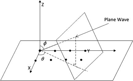
Far-field assumption: For far-field sources, the propagation distance to a sensor array is much larger than the aperture of the array, the DOA parameter is approximately the same to all sensors. According to (14.2), the wave front of constant phase at time instant t is a plane perpendicular to the propagating direction given by ![]() . The term, plane wave assumption is alternatively used in the literature.
. The term, plane wave assumption is alternatively used in the literature.
3.14.2.2 Frequency domain description
In an ideal medium, the propagation between signal sources and a sensor array is considered as a linear time-invariant system. Due to the applicability of the superposition principle and the Fourier transform, the analysis of wave propagation is greatly simplified. In the following, we will develop a general frequency domain model and discuss the narrow band case. The general model is useful for broadband data that may be measured in underwater acoustical or geophysical experiments. The narrow band model is preferred in applications where the signal bandwidth is much smaller than the carrier frequency, for example, wireless communications and radar.
3.14.2.2.1 General model
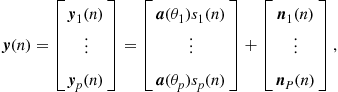
Consider an array of sensors located at ![]() receiving signals generated by P sources. Without loss of generality, the first sensor coincides with the origin of the coordinate system. Let
receiving signals generated by P sources. Without loss of generality, the first sensor coincides with the origin of the coordinate system. Let ![]() denote the signals received by the first sensor. The signal observed by the mth sensor is the sum of a time-delayed version of original signals corrupted by noise
denote the signals received by the first sensor. The signal observed by the mth sensor is the sum of a time-delayed version of original signals corrupted by noise ![]() :
:
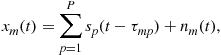 (14.6)
where ![]() denotes the propagation time difference between the origin and the mth sensors. The time difference is given by
denotes the propagation time difference between the origin and the mth sensors. The time difference is given by ![]() where
where ![]() is associated with the pth wave. It is related to the DOA parameter through
is associated with the pth wave. It is related to the DOA parameter through ![]() and (14.5).
and (14.5).
Applying the Fourier transform to the array output ![]() , the time delay
, the time delay ![]() translates to a phase shift
translates to a phase shift ![]() . In the presence of noise, the array output vector
. In the presence of noise, the array output vector ![]() can be written as
can be written as
 (14.7)
where the steering vector ![]() is the spatial signature for the pth incoming wave:
is the spatial signature for the pth incoming wave:
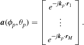 (14.8)
Define the steering matrix as
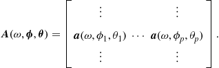 (14.9)
A compact expression for (14.7) is as follows:
![]() (14.10)
(14.10)
where the signal vector ![]() . According to the asymptotic theory of Fourier transform, the frequency domain data is complex normally distributed regardless of the distribution in the time domain. In addition, frequency bins are mutually independent. These properties form the basis for broadband DOA estimation.
. According to the asymptotic theory of Fourier transform, the frequency domain data is complex normally distributed regardless of the distribution in the time domain. In addition, frequency bins are mutually independent. These properties form the basis for broadband DOA estimation.
3.14.2.2.2 Narrow band data
In many applications, the signal of interest is modulated by a carrier frequency ![]() for transmission. At the receive side, the radio frequency signals are demodulated to baseband for further processing. Suppose the signal is band limited with the bandwidth
for transmission. At the receive side, the radio frequency signals are demodulated to baseband for further processing. Suppose the signal is band limited with the bandwidth ![]() , and the maximal travel time between two sensors of the array for a plane wave is
, and the maximal travel time between two sensors of the array for a plane wave is ![]() . The narrow band assumption is valid if
. The narrow band assumption is valid if ![]() . Then the complex baseband signal waveforms are approximately equal for all sensors. The general expression (14.10) can be simplified to the narrow band model
. Then the complex baseband signal waveforms are approximately equal for all sensors. The general expression (14.10) can be simplified to the narrow band model
![]() (14.11)
(14.11)
where the steering matrix ![]() is computed at the carrier frequency
is computed at the carrier frequency ![]() and
and ![]() represents the baseband signal waveform. The frequency dependence in (14.11) is omitted as relevant information is centered at
represents the baseband signal waveform. The frequency dependence in (14.11) is omitted as relevant information is centered at ![]() .
.
As DOA estimation is typically based on sampled values of ![]() at time instants
at time instants ![]() , we consider temporally discrete samples of (14.11) and replace
, we consider temporally discrete samples of (14.11) and replace ![]() with the index n. Then the snapshot model is given by
with the index n. Then the snapshot model is given by
![]() (14.12)
(14.12)
Many array processing methods exploit second order statistics of the data. Assume the signal and noise are independent, stationary random processes with zero mean, correlation matrices ![]() and
and ![]() , respectively where
, respectively where ![]() denotes Hermitian transposition. Then the array correlation matrix can be expressed as
denotes Hermitian transposition. Then the array correlation matrix can be expressed as
![]() (14.13)
(14.13)
The noise process is often considered as spatially white, i.e., ![]() , where
, where ![]() denotes the noise level and
denotes the noise level and ![]() is an
is an ![]() matrix. This assumption is valid for sensors with sufficient spacing. In the presence of colored noise, the noise correlation matrix is no longer diagonal. In such case, the data can be pre-whitened by multiplying (14.12) with the inverse square root of the noise correlation matrix,
matrix. This assumption is valid for sensors with sufficient spacing. In the presence of colored noise, the noise correlation matrix is no longer diagonal. In such case, the data can be pre-whitened by multiplying (14.12) with the inverse square root of the noise correlation matrix, ![]() .
.
The array correlation matrix is estimated from array observations ![]() by the sample correlation matrix
by the sample correlation matrix
 (14.14)
Under weak assumptions, the sample correlation matrix is a consistent estimator for the true correlation matrix, i.e., ![]() converges with probability one to
converges with probability one to ![]() as the sample size increases. More details can be found in the book [8].
as the sample size increases. More details can be found in the book [8].
In many applications, sensors are located on a plane, for example, the yz-plane. Setting the elevation to be ![]() in (14.5), one can easily see that the slowness vector is characterized by only the azimuthal parameter,
in (14.5), one can easily see that the slowness vector is characterized by only the azimuthal parameter, ![]() . In the two dimensional scenario, the uniform linear array (ULA) is one of the most popular array configurations. Let the sensors of a ULA be placed along the y-axis,
. In the two dimensional scenario, the uniform linear array (ULA) is one of the most popular array configurations. Let the sensors of a ULA be placed along the y-axis, ![]() where
where ![]() denotes or the inter-sensor distance. Then the phase shift term evaluated at
denotes or the inter-sensor distance. Then the phase shift term evaluated at ![]() and
and ![]() becomes
becomes ![]() , leading to the steering vector
, leading to the steering vector
![]() (14.15)
(14.15)
If ![]() is measured in wavelength,
is measured in wavelength, ![]() where
where ![]() can be expressed as
can be expressed as
![]() (14.16)
(14.16)
For a standard ULA, the inter-element spacing is half a wavelength, ![]() , the mth element in (14.16) becomes
, the mth element in (14.16) becomes ![]() .
.
For the 2D case, we shall use a shorter notation for the steering matrix, ![]() , in (14.11)–(14.13). More specifically, the sampled array outputs and correlation matrix are expressed as
, in (14.11)–(14.13). More specifically, the sampled array outputs and correlation matrix are expressed as
![]() (14.17)
(14.17)
and
![]() (14.18)
(14.18)
Given the observations ![]() , the primary interest is to estimate the DOA parameter. In the following, we will present DOA estimation methods based on various ideas ranging from nonparametric spectral analysis, high resolution methods to the parametric approach. Our discussion will focus on the mostly investigated 2D case. The majority of the methods can be extended to multiple parameters per source in a straightforward manner. The broadband case will be discussed in detail in a separate chapter.
, the primary interest is to estimate the DOA parameter. In the following, we will present DOA estimation methods based on various ideas ranging from nonparametric spectral analysis, high resolution methods to the parametric approach. Our discussion will focus on the mostly investigated 2D case. The majority of the methods can be extended to multiple parameters per source in a straightforward manner. The broadband case will be discussed in detail in a separate chapter.
3.14.2.3 Uniqueness
A fundamental issue in the direction finding problem is whether the DOA parameters can be identified unambiguously. From the ideal data model (14.12) or (14.17), we know that the array output lies in a subspace spanned by the columns of the ![]() array steering matrix if the noise part
array steering matrix if the noise part ![]() is ignored. For simplicity, we will present the results for the model (14.17). Assume any subset of vectors
is ignored. For simplicity, we will present the results for the model (14.17). Assume any subset of vectors ![]() , are linearly independent. The study in [9,10] specifies the conditions for the maximal number of sources that can be uniquely localized in terms of the number of sensors M and the rank of the signal correlation matrix R. The condition (1)
, are linearly independent. The study in [9,10] specifies the conditions for the maximal number of sources that can be uniquely localized in terms of the number of sensors M and the rank of the signal correlation matrix R. The condition (1) ![]() guarantees uniqueness for every batch of data, while the weaker condition (2)
guarantees uniqueness for every batch of data, while the weaker condition (2) ![]() guarantees uniqueness for almost every batch of data, with the exception of a set of batches of measure zero. When all sources are uncorrelated implying that
guarantees uniqueness for almost every batch of data, with the exception of a set of batches of measure zero. When all sources are uncorrelated implying that ![]() , condition (1) is always satisfied and uniqueness is always guaranteed. When the sources are fully correlated,
, condition (1) is always satisfied and uniqueness is always guaranteed. When the sources are fully correlated, ![]() , then uniqueness is ensured if
, then uniqueness is ensured if ![]() by condition (1). The weaker condition (2) leads to a less stringent condition
by condition (1). The weaker condition (2) leads to a less stringent condition ![]() . Details on the proof are to be found in [10].
. Details on the proof are to be found in [10].
3.14.3 Beamforming methods
A homogenous wavefield ![]() has an interpretation as energy distribution in a frequency-wavenumber spectrum. The power spectrum of
has an interpretation as energy distribution in a frequency-wavenumber spectrum. The power spectrum of ![]() contains information about the source distribution over space [3]. From this perspective, estimation of DOA parameters is equivalent to finding the location in a spatial power spectrum where most power is concentrated. Beamforming techniques are spatial filters that combine weighted sensor outputs linearly
contains information about the source distribution over space [3]. From this perspective, estimation of DOA parameters is equivalent to finding the location in a spatial power spectrum where most power is concentrated. Beamforming techniques are spatial filters that combine weighted sensor outputs linearly
 (14.19)
where ![]() . The weight vector is usually a function of the DOA parameter, i.e.,
. The weight vector is usually a function of the DOA parameter, i.e., ![]() . The power of the beamformer output
. The power of the beamformer output ![]() provides an estimate for the power spectrum at the direction
provides an estimate for the power spectrum at the direction ![]() :
:
 (14.20)
where ![]() is the sample covariance matrix. The maximum of
is the sample covariance matrix. The maximum of ![]() is an indication for a signal source. Assuming P signals are present in the wavefield, we change the look direction
is an indication for a signal source. Assuming P signals are present in the wavefield, we change the look direction ![]() and evaluate
and evaluate ![]() over the range of interest. Then the P largest maxima are chosen as DOA estimates.
over the range of interest. Then the P largest maxima are chosen as DOA estimates.
The expected beamformer output (14.20) is a smoothed version of the true power spectrum. Smoothing is carried out with the kernel ![]() centered at the look direction
centered at the look direction ![]() , where
, where ![]() is the array beam pattern [3]. An ideal beam pattern
is the array beam pattern [3]. An ideal beam pattern ![]() would lead to an unbiased estimate for the power spectrum. However, in practice, due to finite array aperture, the beampattern consists of a main lobe and several sidelobes, leading to leakage from neighboring frequencies. Hence, the shape of the beampattern determines resolution capability and estimation accuracy of the spectral analysis based approach.
would lead to an unbiased estimate for the power spectrum. However, in practice, due to finite array aperture, the beampattern consists of a main lobe and several sidelobes, leading to leakage from neighboring frequencies. Hence, the shape of the beampattern determines resolution capability and estimation accuracy of the spectral analysis based approach.
We will introduce the conventional beamformer in Section 3.14.3.1 and minimum variance distortionless (MVDR) beamformer in Section 3.14.3.2, respectively. A recently proposed sparse data approach that matches array measurements to a set of candidate directions will be discussed in Section 3.14.3.3.
3.14.3.1 Conventional beamformer
The conventional beamformer, also termed as delay-and-sum beamformer, combines the output of each sensor (14.6) coherently to obtain an enhanced signal from the noisy observation. For simplicity, assume ![]() for now. In its most general form, the conventional beamformer compensates the time delayed observation at the mth sensor
for now. In its most general form, the conventional beamformer compensates the time delayed observation at the mth sensor ![]() by the amount of
by the amount of ![]() . The sum of aligned sensor outputs leads to an estimate for the signal:
. The sum of aligned sensor outputs leads to an estimate for the signal:
 (14.21)
From the above equation, it is clear that the signal to noise ratio is improved by a factor of M. For wideband data, the sum in (14.21) is often called true time-delay beamforming. It can be approximately implemented using various filtering techniques, see e.g., [6,7]. For narrow band data, the shift in the time domain becomes phase shift in the frequency domain. Therefore, we have
 (14.22)
where ![]() is the steering vector evaluated at the look direction
is the steering vector evaluated at the look direction ![]() . Since for any steering vectors,
. Since for any steering vectors, ![]() , the weight vector has unit length
, the weight vector has unit length ![]() and
and
 (14.23)
An estimate for the power spectrum is then obtained as
![]() (14.24)
(14.24)
In the context of spectral analysis, the above expression corresponds to the periodogram in the spatial domain [3]. The expected value of ![]() is the convolution between the beam pattern and the true power spectrum. A good beam pattern should be as close to the delta function
is the convolution between the beam pattern and the true power spectrum. A good beam pattern should be as close to the delta function ![]() as possible to minimize leakage from neighboring frequencies.
as possible to minimize leakage from neighboring frequencies.
For a uniform linear array, the beam pattern ![]() has a main lobe around the look direction
has a main lobe around the look direction ![]() . The Rayleigh beamwidth, the distance between the first two nulls of
. The Rayleigh beamwidth, the distance between the first two nulls of ![]() , is approximately given by
, is approximately given by
![]() (14.25)
(14.25)
The beamformer can only distinguish two sources with DOA separation larger than half of ![]() . Note that
. Note that ![]() is the ratio between actual distance D and wavelength
is the ratio between actual distance D and wavelength ![]() . As
. As ![]() is inversely proportional to Md, the aperture of the array, the resolution capability improves with increasing number of sensors and sensor spacing. However,
is inversely proportional to Md, the aperture of the array, the resolution capability improves with increasing number of sensors and sensor spacing. However, ![]() is the maximally allowed sensor distance. For
is the maximally allowed sensor distance. For ![]() , grating lobes appear in the beampattern and create ambiguity in the DOA estimation.
, grating lobes appear in the beampattern and create ambiguity in the DOA estimation.
For a standard ULA with ![]() sensors,
sensors, ![]() , the beamwidth
, the beamwidth ![]() , meaning that the DOA separation between two sources must be larger than 11° to generate two peaks in the power spectrum
, meaning that the DOA separation between two sources must be larger than 11° to generate two peaks in the power spectrum ![]() .
.
3.14.3.2 Minimum variance distortionless response (MVDR) beamformer
The minimum variance distortionless response (MVDR) beamformer [1] alleviates the resolution limit of the conventional beamformer by considering the following constrained optimization problem:
![]() (14.26)
(14.26)
![]() (14.27)
(14.27)
The objective function (14.26) represents the output power to be minimized. The constraint (14.27) ensures that signals from the desired direction ![]() remain undistorted. In other words, while the power from all other directions is minimized, the beamformer concentrates only on the look direction. The behavior of the MVDR beamformer was also discussed by Lacoss [11]. The resulting beampattern has a sharp peak at the target DOA, leading to resolution capability beyond the Rayleigh beamwidth. Applying the method of Lagrange multipliers, we obtain the solution as
remain undistorted. In other words, while the power from all other directions is minimized, the beamformer concentrates only on the look direction. The behavior of the MVDR beamformer was also discussed by Lacoss [11]. The resulting beampattern has a sharp peak at the target DOA, leading to resolution capability beyond the Rayleigh beamwidth. Applying the method of Lagrange multipliers, we obtain the solution as
 (14.28)
Replacing (14.28) into (14.20), one obtains the power function as
![]() (14.29)
(14.29)
A condition on the MVDR beamformer follows immediately from (14.28) where the inversion of the sample covariance matrix requires that ![]() is full rank, implying that the number of samples must be larger than the number of sensors, i.e.,
is full rank, implying that the number of samples must be larger than the number of sensors, i.e., ![]() . When rank deficiency occurs or the sample number is small compared to the number of sensors, a popular technique known as diagonal loading is often employed to improve robustness. As the name implies, the sample covariance matrix (14.14) is modified by adding a small perturbation term to improve the conditioning:
. When rank deficiency occurs or the sample number is small compared to the number of sensors, a popular technique known as diagonal loading is often employed to improve robustness. As the name implies, the sample covariance matrix (14.14) is modified by adding a small perturbation term to improve the conditioning:
 (14.30)
where ![]() is a properly chosen small number and
is a properly chosen small number and ![]() is an
is an ![]() identity matrix. The choice of the coefficient
identity matrix. The choice of the coefficient ![]() is essential. Several criteria for optimal choice of diagonal loading have been reported in [12] and the references therein.
is essential. Several criteria for optimal choice of diagonal loading have been reported in [12] and the references therein.
A variant of the MVDR beamformer, proposed in [13], replaces the constraint (14.27) by ![]() . This formulation leads to the adapted angular response spectrum
. This formulation leads to the adapted angular response spectrum ![]() . This Borgiorri-Kaplan beamformer is known to provide higher spatial resolution than that of the MVDR beamformer. In [14], the denominator of (14.29) is replaced by
. This Borgiorri-Kaplan beamformer is known to provide higher spatial resolution than that of the MVDR beamformer. In [14], the denominator of (14.29) is replaced by ![]() where
where ![]() . Simulation results therein show that using higher order covariance matrix has superior resolution capability and robustness against signal correlation and low SNR.
. Simulation results therein show that using higher order covariance matrix has superior resolution capability and robustness against signal correlation and low SNR.
The performance of the MVDR beamformer depends on the number of snapshots, array aperture, and SNR. Several interesting results are reported in [15]. In the presence of coherent or strongly correlated interferences, the performance of the MVDR beamformer degrades dramatically. Alternative methods addressing this issue are reported in [16–21]. Due to the distortionless response constraint, the MVDR beamformer is sensitive to errors in the target direction and array response imperfection. Robust methods to tackle this problem have been suggested in [22,23].
3.14.3.3 Sparse data representation based approach
The beamforming methods localize the signal sources by estimating the power spectrum associated with various DOAs. Since the number of signals is usually small in array processing, the methods proposed in [24,25] view DOA estimation as sparse data reconstruction and assign DOA estimates to signals with nonzero amplitude. In this approach, the first step is to find a sparse representation of the array output data. The beamforming output in the frequency domain [24] or the array observation (14.12) [25] can be used to construct a sparse data representation. Then the underlying optimization problem (typically convex) will be solved to find nonzero components. DOA estimates are obtained from angles associated with nonzero components. Recently this approach has attracted many researchers’ attention thanks to advances in the theory and methodology of sparse data reconstruction [26].
For representational convenience, we follow the formulation in [25]. Let ![]() be a sampling grid of source locations of interest. An important assumption here is that the number of signals is much smaller than the number of sample grids, i.e.,
be a sampling grid of source locations of interest. An important assumption here is that the number of signals is much smaller than the number of sample grids, i.e., ![]() . The overcomplete array manifold matrix
. The overcomplete array manifold matrix ![]() consists of
consists of ![]() steering vectors. The
steering vectors. The ![]() signal vector
signal vector ![]() has a nonzero component
has a nonzero component ![]() if a signal source is present at
if a signal source is present at ![]() . For a single snapshot, the array output (14.12) can be re-expressed in terms of the sparse vector
. For a single snapshot, the array output (14.12) can be re-expressed in terms of the sparse vector ![]() as:
as:
![]() (14.31)
(14.31)
Now the problem reduces to finding the nonzero component in ![]() . In the noiseless case, the ideal measure would be
. In the noiseless case, the ideal measure would be ![]() which counts the nonzero entries. This would in fact lead to the deterministic ML method over a grid search. But this metric will lead to a complicated combinatorial optimization problem. Therefore, one tries to approximate the solution by using
which counts the nonzero entries. This would in fact lead to the deterministic ML method over a grid search. But this metric will lead to a complicated combinatorial optimization problem. Therefore, one tries to approximate the solution by using ![]() norm,
norm, ![]() . The significant advantage of
. The significant advantage of ![]() relaxation is that the convex optimization problem,
relaxation is that the convex optimization problem,
![]() (14.32)
(14.32)
has a unique global minimum and can be solved by computationally efficient numerical methods such as linear programming. For noisy measurements (14.31), the constraint ![]() can not hold and needs to be relaxed. An appropriate objective function is suggested in [24,25]
can not hold and needs to be relaxed. An appropriate objective function is suggested in [24,25]
![]() (14.33)
(14.33)
where ![]() is a regularization parameter.
is a regularization parameter.
For multiple snapshots, we define the data matrix ![]() , the signal matrix
, the signal matrix ![]() and the noise matrix
and the noise matrix ![]() . They are related as follows:
. They are related as follows:
![]() (14.34)
(14.34)
To measure sparsity for multiple time samples, we define the ith row vector of ![]() corresponding to a particular DOA grid point
corresponding to a particular DOA grid point ![]() as
as ![]() and compute its
and compute its ![]() norm
norm ![]() . Then the spatial sparsity is imposed on the
. Then the spatial sparsity is imposed on the ![]() vector
vector ![]() . The multiple sample version of (14.33) becomes
. The multiple sample version of (14.33) becomes
![]() (14.35)
(14.35)
where ![]() is the Forbenius norm. The regularization parameter
is the Forbenius norm. The regularization parameter ![]() is a tradeoff between the fit to data and the sparsity. In [24,25], statistically motivated strategies for selecting
is a tradeoff between the fit to data and the sparsity. In [24,25], statistically motivated strategies for selecting ![]() are discussed.
are discussed.
The computational cost for solving (14.35) increases significantly with the number of snapshots N. A coherent combination based on singular value decomposition (SVD) of the data matrix is suggested in [25]. A mixed norm approach for joint recovery is proposed in [27]. This problem can be avoided when other forms of sparsity are used, for example, the beamforming output in [24] and the covariance matrix in [28]. The resolution capability of this approach is investigated in [29].
Simulation results in the above mentioned references show that the sparse data representation based approach has a much better resolution than the conventional and MVDR beamformers at the expense of increased computational cost. Another advantage over the subspace methods is the improved robustness against signal coherence. However, for low SNRs and closely located sources, the relatively high bias remains an challenging issue for this approach.
3.14.3.4 Numerical examples
In this section, the beamforming based methods discussed previously are tested by numerical experiments. In the simulation, a uniform linear array of 12 sensors with inter-element spacings of half a wavelength is employed. The narrow band signals are generated by ![]() uncorrelated signals of various strengths. The signal to noise ratio of the first and second signals are given by [5 0] dB, respectively. The number of snapshots is
uncorrelated signals of various strengths. The signal to noise ratio of the first and second signals are given by [5 0] dB, respectively. The number of snapshots is ![]() in each Monte Carlo trial.
in each Monte Carlo trial.
Figure 14.2 shows the normalized spectra obtained from conventional beamformer, MVDR beamformer and sparse data representation over ![]() to
to ![]() for well separated sources located
for well separated sources located ![]() relative to the broadside. All the three methods exhibit two peaks at the reference locations. For the second experiment, the reference DOA parameter is given by
relative to the broadside. All the three methods exhibit two peaks at the reference locations. For the second experiment, the reference DOA parameter is given by ![]() , which corresponds to closely located signals. As shown in Figure 14.3, the conventional beamformer only leads to one maximum between the true DOAs and does not recognize the existence of two signals. On the other hand, the MVDR beamformer and the sparse data representation based approach perform well in resolving two signals.
, which corresponds to closely located signals. As shown in Figure 14.3, the conventional beamformer only leads to one maximum between the true DOAs and does not recognize the existence of two signals. On the other hand, the MVDR beamformer and the sparse data representation based approach perform well in resolving two signals.

Figure 14.2 Normalized spectrum for well separated signals. Reference DOA parameter ![]() , SNR = [5 0] dB,
, SNR = [5 0] dB, ![]() .
.

Figure 14.3 Normalized spectrum for closely located signals. Reference DOA parameter ![]() , SNR = [5 0] dB,
, SNR = [5 0] dB, ![]() .
.
In the third experiment, we compare the estimation accuracy of these methods. To avoid resolution problem, the reference DOA parameter is chosen as ![]() . Both signals have equal power with SNR running from −5 dB to 20 dB in a 1 dB step. Figure 14.4 depicts the root mean squared error (RMSE) obtained from 1000 trials. For all three methods, RMSE decreases with increasing SNR. The sparse data representation based method has an overall best performance over the entire SNR range. The MVDR beamformer lies between the other two methods. The gap between these methods becomes most significant at low SNRs. For example, at SNR = −5 dB, the RMSE of conventional beamformer is
. Both signals have equal power with SNR running from −5 dB to 20 dB in a 1 dB step. Figure 14.4 depicts the root mean squared error (RMSE) obtained from 1000 trials. For all three methods, RMSE decreases with increasing SNR. The sparse data representation based method has an overall best performance over the entire SNR range. The MVDR beamformer lies between the other two methods. The gap between these methods becomes most significant at low SNRs. For example, at SNR = −5 dB, the RMSE of conventional beamformer is ![]() which is more than three times that of the sparse data representation based method with RMSE = 1.5°.
which is more than three times that of the sparse data representation based method with RMSE = 1.5°.
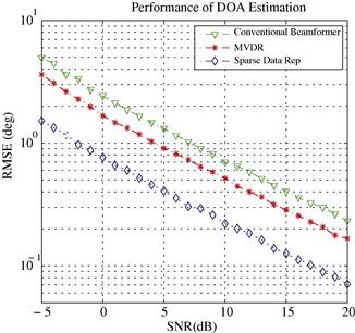
From the simulation results, we have observed the resolution limitation of the conventional beamformer. Improved resolution capability and estimation accuracy can be achieved by the MVDR beamformer and computationally involved sparse data representation based estimator.
3.14.4 Subspace methods
In an attempt to overcome the resolution limit of conventional beamforming, many spectral-like methods were introduced in seventies. They exploit the eigenstructure of the spatial correlation matrix (14.18) to form pseudo spectrum functions. These functions exhibit sharp peaks at the true parameters and lead to superior performance as compared to the Fourier based analysis. While the early work by Pisarenko [30] was devoted to harmonic retrieval, the MUSIC (Multiple SIgnal Classification) algorithm [2,31] was developed for array signal processing.
Recall that ![]() is a Hermitian symmetric matrix. Therefore, the eigenvectors are orthogonal. From (14.18), it is apparent that the eigenvalues induced by the signal part differs from the remaining ones by the noise level. More specifically, let
is a Hermitian symmetric matrix. Therefore, the eigenvectors are orthogonal. From (14.18), it is apparent that the eigenvalues induced by the signal part differs from the remaining ones by the noise level. More specifically, let ![]() denote eigenvalue/eigenvector pairs of
denote eigenvalue/eigenvector pairs of ![]() , the spectral decomposition of
, the spectral decomposition of ![]() can be expressed as
can be expressed as
 (14.36)
where ![]() and
and ![]() . When the signal covariance matrix
. When the signal covariance matrix ![]() is full rank, i.e.,
is full rank, i.e., ![]() , the matrix
, the matrix ![]() has the rank of P. The eigenvalues satisfy the property:
has the rank of P. The eigenvalues satisfy the property: ![]() . The signal eigenvectors corresponding to the P largest eigenvalues span the same subspace as the steering matrix. The noise eigenvectors corresponding to the remaining
. The signal eigenvectors corresponding to the P largest eigenvalues span the same subspace as the steering matrix. The noise eigenvectors corresponding to the remaining ![]() eigenvalues are orthogonal to the signal subspace. Mathematically, the signal and noise subspaces are related to the steering matrix as follows:
eigenvalues are orthogonal to the signal subspace. Mathematically, the signal and noise subspaces are related to the steering matrix as follows:
![]() (14.37)
(14.37)
In practice, the analysis is based on the sample covariance matrix ![]() . The eigenvalues and eigenvectors in (14.36) are then replaced by their estimates
. The eigenvalues and eigenvectors in (14.36) are then replaced by their estimates ![]() . Similarly, the matrices on the right hand side of (14.36) are substituted by corresponding estimates
. Similarly, the matrices on the right hand side of (14.36) are substituted by corresponding estimates ![]() and
and ![]() , respectively. For finite samples,
, respectively. For finite samples, ![]() and
and ![]() , the property (14.37) is approximately valid. Many efforts have been made to find the best way of combining the estimated signal and noise eigenvectors to achieve high resolution capability and estimation accuracy. In the following, we assume that the number of signals is known so that the signal and noise subspaces can be separated. Methods for determination of the number of sources will be discussed separately in Section 3.14.7. In the following, we will present the well known MUSIC and ESPRIT algorithms in Sections 3.14.4.1 and 3.14.4.2, respectively. The important issue of signal coherence will be discussed in Section 3.14.4.3.
, the property (14.37) is approximately valid. Many efforts have been made to find the best way of combining the estimated signal and noise eigenvectors to achieve high resolution capability and estimation accuracy. In the following, we assume that the number of signals is known so that the signal and noise subspaces can be separated. Methods for determination of the number of sources will be discussed separately in Section 3.14.7. In the following, we will present the well known MUSIC and ESPRIT algorithms in Sections 3.14.4.1 and 3.14.4.2, respectively. The important issue of signal coherence will be discussed in Section 3.14.4.3.
3.14.4.1 MUSIC
The MUSIC algorithm suggested by Schmidt [2,32], and Bienvenu and Kopp [31] exploits the orthogonality between signal and noise subspaces. From (14.37), we know that any vector ![]() satisfies
satisfies
![]() (14.38)
(14.38)
Assume the array is unambiguous; that is, any collection of P distinct DOAs ![]() forms a linearly independent set
forms a linearly independent set ![]() . Then the above relation is valid for P distinct columns of
. Then the above relation is valid for P distinct columns of ![]() . Motivated by this observation, the MUSIC spectrum is defined in terms of the estimated noise eigenvectors as
. Motivated by this observation, the MUSIC spectrum is defined in terms of the estimated noise eigenvectors as
![]() (14.39)
(14.39)
For high SNR (or large N) and uncorrelated signal sources, the MUSIC spectrum exhibits high peaks near the true DOAs. To find the DOA estimates, we calculate ![]() over a fine grid of
over a fine grid of ![]() and locate the P largest maxima of
and locate the P largest maxima of ![]() . In comparison with the MVDR beamformer (14.29), the MUSIC spectrum uses the projection matrix
. In comparison with the MVDR beamformer (14.29), the MUSIC spectrum uses the projection matrix ![]() rather than
rather than ![]() . To get more insight, assume a perfect spatial correlation matrix. Then, for noise eigenvalues
. To get more insight, assume a perfect spatial correlation matrix. Then, for noise eigenvalues ![]() and
and ![]() approaches
approaches ![]() . Then MUSIC may be interpreted as a MVDR-like method with a correlation matrix calculated at infinite SNR. This explains the superior resolution of MUSIC than MVDR [3].
. Then MUSIC may be interpreted as a MVDR-like method with a correlation matrix calculated at infinite SNR. This explains the superior resolution of MUSIC than MVDR [3].
In [33,34], an alternative implementation of MUSIC is suggested to improve estimation accuracy. The idea behind the sequential MUSIC is to find the strongest signal in each iteration and then remove the estimated signal from the observation for the next iteration. As theoretical analysis and numerical results in [34] show the advantage of sequential MUSIC over standard MUSIC is significant for correlated signals. The Toeplitz approximation method [35] provides another implementation of MUSIC specific to uncorrelated sources with a ULA.
For a uniform linear array, MUSIC has a simple implementation. Let ![]() where
where ![]() , the steering vector (14.16) has the form:
, the steering vector (14.16) has the form:
![]() (14.40)
(14.40)
The inverse of the MUSIC spectrum (14.39) becomes
![]() (14.41)
(14.41)
The root-MUSIC algorithm [36] finds the roots of the complex polynomial function ![]() rather than searching for maxima of the MUSIC spectrum. Among the
rather than searching for maxima of the MUSIC spectrum. Among the ![]() possible candidates, P roots
possible candidates, P roots ![]() that are closest to the unit circle on the complex plane are selected to obtain DOA estimates. Since
that are closest to the unit circle on the complex plane are selected to obtain DOA estimates. Since ![]() , the DOA parameters are given by
, the DOA parameters are given by ![]() . It is known that root-MUSIC has the same asymptotic performance as standard MUSIC. In the finite sample case, root-MUSIC has a much better threshold behavior and improved resolution capability [37]. This is explained by the fact that the radial component of the errors in
. It is known that root-MUSIC has the same asymptotic performance as standard MUSIC. In the finite sample case, root-MUSIC has a much better threshold behavior and improved resolution capability [37]. This is explained by the fact that the radial component of the errors in ![]() will not affect
will not affect ![]() . Since the search procedure in standard MUSIC is replaced by solving the roots of a polynomial in root-MUSIC, the computational cost is significantly reduced. However, while standard MUSIC is applicable to arbitrary array geometry, root-MUSIC requires a ULA. When ULAs are not available, one can apply array interpolation techniques [38] to approximate the array response. For more details on array interpolation, the reader is referred to Chapter 16 of this book.
. Since the search procedure in standard MUSIC is replaced by solving the roots of a polynomial in root-MUSIC, the computational cost is significantly reduced. However, while standard MUSIC is applicable to arbitrary array geometry, root-MUSIC requires a ULA. When ULAs are not available, one can apply array interpolation techniques [38] to approximate the array response. For more details on array interpolation, the reader is referred to Chapter 16 of this book.
The extension of standard MUSIC to the two dimensional case is straightforward. The 2D steering vector (14.8) is used in the MUSIC spectrum, searching for the P largest maxima over a two dimensional space. For root-MUSIC, an additional ULA is required to be able to resolve both azimuth and elevation [39]. More algorithms and results regarding two dimensional DOA estimation are to be found in Chapter 15 of this book.
While the MUSIC algorithm utilizes all noise eigenvectors, the Minimum Norm (Min-Norm) algorithm suggested in [40,41] uses a single vector in the noise space. A comprehensive study on the resolution capability of MUSIC and the Min-Norm algorithm can be found in [42].
3.14.4.2 ESPRIT
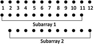
The ESPRIT (Estimation of Signal Parameters via Rotational Invariance Techniques) algorithm proposed by Roy and Kailath [43] exploits the rotational invariance property of two identical subarrays and solves the eigenvalues of a matrix relating two signal subspaces. A simple way to construct identical subarrays is to select the first ![]() elements and the second to the Mth elements of a ULA (see Figure 14.5). The array response matrices of the first and second subarrays are then expressed as
elements and the second to the Mth elements of a ULA (see Figure 14.5). The array response matrices of the first and second subarrays are then expressed as
![]() (14.42)
(14.42)
where ![]() and
and ![]() are selection matrices of the first and second subarrays. They consist of an
are selection matrices of the first and second subarrays. They consist of an ![]() identity matrix and an
identity matrix and an ![]() zero vector
zero vector
![]() (14.43)
(14.43)
Define ![]() . From (14.42), we know that the two subarrays have the same array response up to a phase shift due to the distance between them. This observation leads to the shift invariance property
. From (14.42), we know that the two subarrays have the same array response up to a phase shift due to the distance between them. This observation leads to the shift invariance property
![]() (14.44)
(14.44)
where ![]() . Note that ESPRIT is applicable for array geometries other than ULAs as long as the shift invariance property holds, see e.g., [43–45].
. Note that ESPRIT is applicable for array geometries other than ULAs as long as the shift invariance property holds, see e.g., [43–45].
Recall that the signal subspace of the original array and the signal eigenvectors span the same subspace; therefore, they are related through a nonsingular linear transformation ![]() :
:
![]() (14.45)
(14.45)
Multiplying both sides of (14.45) with ![]() and
and ![]() ,
,
![]() (14.46)
(14.46)
Combining (14.44) and (14.46) yields the relation between ![]() and
and ![]() :
:
![]() (14.47)
(14.47)
Since the matrix ![]() is similar to the diagonal matrix
is similar to the diagonal matrix ![]() , both matrices have the same eigenvalues,
, both matrices have the same eigenvalues, ![]() .
.
Using estimates ![]() in (14.47), one can apply LS (Least Squares) or TLS (Total Least Squares) to obtain
in (14.47), one can apply LS (Least Squares) or TLS (Total Least Squares) to obtain ![]() [46]. Finally, DOA estimates are obtained from eigenvalues of
[46]. Finally, DOA estimates are obtained from eigenvalues of ![]() by the formula
by the formula ![]() . The computational burden of the ESPRIT algorithm can be reduced by using real-valued operations as proposed in [44].
. The computational burden of the ESPRIT algorithm can be reduced by using real-valued operations as proposed in [44].
3.14.4.3 Signal coherence
In the development of subspace methods, we have made an important assumption that the rank of the signal covariance matrix ![]() equals the number of signals P so that the signal eigenvectors spans the same subspace as the column space of the array manifold matrix. However, this condition no longer holds when two signals are coherent, meaning that the magnitude of the correlation coefficient of the signals is one. Coherent signals are often encountered in wireless communications as a result of a multipath propagation effect or smart jamming in radar systems. In the presence of signal coherence,
equals the number of signals P so that the signal eigenvectors spans the same subspace as the column space of the array manifold matrix. However, this condition no longer holds when two signals are coherent, meaning that the magnitude of the correlation coefficient of the signals is one. Coherent signals are often encountered in wireless communications as a result of a multipath propagation effect or smart jamming in radar systems. In the presence of signal coherence, ![]() becomes rank deficient, leading to divergence of signal eigenvectors into the noise subspace. Since the property (14.38) is not satisfied, performance of subspace methods degrades significantly. To mitigate the effect of signal coherence, one could apply forward-backward averaging or spatial smoothing techniques. The former requires a ULA and can handle two coherent signals. The latter requires arrays with a translational invariance property and is able to deal with maximally P coherent signals.
becomes rank deficient, leading to divergence of signal eigenvectors into the noise subspace. Since the property (14.38) is not satisfied, performance of subspace methods degrades significantly. To mitigate the effect of signal coherence, one could apply forward-backward averaging or spatial smoothing techniques. The former requires a ULA and can handle two coherent signals. The latter requires arrays with a translational invariance property and is able to deal with maximally P coherent signals.
Let ![]() denote the exchange matrix comprised of ones on the anti-diagonal and zeros elsewhere. For a ULA, the steering vector (14.16) has an interesting property:
denote the exchange matrix comprised of ones on the anti-diagonal and zeros elsewhere. For a ULA, the steering vector (14.16) has an interesting property:
![]() (14.48)
(14.48)
which implies
![]() (14.49)
(14.49)
where ![]() . The backward covariance is defined as
. The backward covariance is defined as
![]() (14.50)
(14.50)
The forward-backward covariance matrix is obtained by averaging of ![]() and the standard array covariance matrix
and the standard array covariance matrix ![]() :
:
![]() (14.51)
(14.51)
Applying the property (14.49), the modified signal covariance matrix is then given by
![]() (14.52)
(14.52)
The coherent signals are de-correlated through phase modulation by the diagonal elements of ![]() . The forward-backward ESPRIT is equivalent to the unitary ESPRIT [44], because it only uses real valued components.
. The forward-backward ESPRIT is equivalent to the unitary ESPRIT [44], because it only uses real valued components.
In a general case where more than two coherent signals are present, we need a more powerful solution to restore the rank of the signal covariance matrix. The spatial smoothing technique, first proposed in [47] and extended in [38,48,49], exploits the degrees of freedom of a regular array by splitting it into several identical subarrays. Let ![]() denote the number of sensors of a subarray. For a ULA of M elements, the maximal number of subarrays is
denote the number of sensors of a subarray. For a ULA of M elements, the maximal number of subarrays is ![]() . The array response matrix of the lth subarray is related to
. The array response matrix of the lth subarray is related to ![]() as
as
![]() (14.53)
(14.53)
where the selection matrix is ![]() . The spatially averaged covariance matrix is then given by
. The spatially averaged covariance matrix is then given by
 (14.54)
In the case of a ULA, one can combine the forward-backward averaging (14.51) with the spatial smoothing. In [48,50], it was shown that under mild conditions, the signal covariance matrix obtained from forward-backward averaging and spatial smoothing is nonsingular. Since the subarrays have a smaller aperture than the original array, the signal coherency is removed at the expense of resolution capability. The two dimensional extension of spatial smoothing is addressed in [51–53].
3.14.4.4 Numerical examples
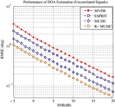
We demonstrate the performance of the subspace methods presented previously by numerical results. A uniform linear array of 12 sensors with inter-element spacings of half a wavelength is employed. In this case, the application of root-MUSIC is straightforward. Narrow band signals are generated by ![]() well separated sources of equal strengths located at
well separated sources of equal strengths located at ![]() . The number of snapshots is
. The number of snapshots is ![]() . Both signals are equal power with SNR running from −5 dB to 20 dB. The two subarrays used in ESPRIT are ULAs comprised of 11 elements.
. Both signals are equal power with SNR running from −5 dB to 20 dB. The two subarrays used in ESPRIT are ULAs comprised of 11 elements.
In the first experiment, we consider uncorrelated signals. For comparison, the MVDR beamformer is applied to the same batch of data. The empirical RMSE is obtained from 1000 trials. From Figure 14.6, one can observe that root-MUSIC, denoted by R-MUSIC, outperforms standard MUSIC and ESPRIT. All the subspace methods have lower estimation errors than the MVDR beamformer. The performance difference is most significant at low SNRs. For SNR close to 20 dB, all methods behave similarly. The superior performance of root-MUSIC compared to standard MUSIC is expected as predicted by the theoretical analysis [37]. The estimation error of ESPRIT is higher than both MUSIC algorithms due to the reduced aperture.
In the second experiment, two correlated signals are considered with real valued correlation coefficient ![]() . One can observe from Figure 14.7 that the performance of all methods degrade rapidly. At
. One can observe from Figure 14.7 that the performance of all methods degrade rapidly. At ![]() , the RMSE is more than twice the RMSE in the uncorrelated case. Both MUSIC-based algorithms have almost identical performance. They are slightly better than ESPRIT. The curve of ESPRIT almost coincides with that of MVDR. These observations indicate that subspace methods are very sensitive to signal correlation and can not provide accurate estimates when rank deficiency occurs. If we use the forward-backward averaged sample covariance matrix (14.51) in the subspace methods, denoted by FB-ESPRIT, FB-MUSIC, and FB-R-MUSIC, respectively, the estimation accuracy improves significantly as the three curves at the bottom show. In comparison with Figure 14.6, the RMSE increases only slightly when the FB technique is applied. For a detailed discussion on highly correlated signals, the reader is referred to Chapter 15 of this book.
, the RMSE is more than twice the RMSE in the uncorrelated case. Both MUSIC-based algorithms have almost identical performance. They are slightly better than ESPRIT. The curve of ESPRIT almost coincides with that of MVDR. These observations indicate that subspace methods are very sensitive to signal correlation and can not provide accurate estimates when rank deficiency occurs. If we use the forward-backward averaged sample covariance matrix (14.51) in the subspace methods, denoted by FB-ESPRIT, FB-MUSIC, and FB-R-MUSIC, respectively, the estimation accuracy improves significantly as the three curves at the bottom show. In comparison with Figure 14.6, the RMSE increases only slightly when the FB technique is applied. For a detailed discussion on highly correlated signals, the reader is referred to Chapter 15 of this book.

3.14.5 Parametric methods
The spectral-like methods presented previously treat the direction finding problem as spatial frequency estimation. Although subspace methods overcome the resolution limitation of beamforming techniques, and yield good estimates at reasonable computational cost, the performance degrades dramatically in the presence of correlated or coherent signals. Parametric methods exploit the data model directly and are usually statistically well motivated. The well known maximum likelihood (ML) approach is representative of this class of estimators. Since parametric methods are not dependent on the eigenstructure of the sample covariance matrix, they provide reasonable results in scenarios involving signal correlation/coherence, low SNRs and small data samples. The price for the improved robustness and accuracy is the increased computational complexity. We will introduce the maximum likelihood approach and the covariance matching estimation methods in Sections 3.14.5.1 and 3.14.5.4, respectively. Several numerical algorithms for efficient implementation of the ML estimator will be presented in Section 3.14.5.2. Analytical results on the performance of DOA estimators presented so far will be discussed in Section 3.14.5.5.
3.14.5.1 The maximum likelihood approach
The maximum likelihood method is a systematic tool for constructing estimators. Based on the statistical model for data samples, it maximizes the likelihood function over the parameters of interest to derive estimates. The well known properties of ML estimation include asymptotic normality and efficiency under proper conditions [54]. For DOA estimation, the application is straightforward. Recall the data model in (14.17)
![]() (14.55)
(14.55)
We assume the noise ![]() is temporally independent and complex normally distributed with zero mean and covariance matrix
is temporally independent and complex normally distributed with zero mean and covariance matrix ![]() , i.e.,
, i.e., ![]() . In the array processing literature, two different interpretations of the source signals lead to the deterministic and the stochastic ML estimators.
. In the array processing literature, two different interpretations of the source signals lead to the deterministic and the stochastic ML estimators.
3.14.5.1.1 Deterministic maximum likelihood
In the deterministic ML approach, the signal ![]() is viewed as a fixed realization of a stochastic process; the parameters
is viewed as a fixed realization of a stochastic process; the parameters ![]() are considered to be deterministic and unknown. With the above noise assumption, the array output
are considered to be deterministic and unknown. With the above noise assumption, the array output ![]() is complex normally distributed with mean
is complex normally distributed with mean ![]() and covariance matrix
and covariance matrix ![]() , i.e.,
, i.e., ![]() . Because the array outputs
. Because the array outputs ![]() are independent, the joint likelihood function is the product of the likelihood associated with each snapshot, i.e.,
are independent, the joint likelihood function is the product of the likelihood associated with each snapshot, i.e.,
 (14.56)
where ![]() denotes the Euclidean norm. The log-likelihood function is then given by
denotes the Euclidean norm. The log-likelihood function is then given by
 (14.57)
The unknown parameters ![]() include the DOA parameter and nuisance parameters. As the number of the signal waveform parameters increases with increasing number of snapshots, the high dimension of parameter space will make direct optimization of (14.57) infeasible. It is well known that the likelihood function is separable [55,3], and the likelihood can be concentrated with respect to the linear parameters. For a fixed, unknown
include the DOA parameter and nuisance parameters. As the number of the signal waveform parameters increases with increasing number of snapshots, the high dimension of parameter space will make direct optimization of (14.57) infeasible. It is well known that the likelihood function is separable [55,3], and the likelihood can be concentrated with respect to the linear parameters. For a fixed, unknown ![]() , the ML estimate of the signal is given by
, the ML estimate of the signal is given by
![]() (14.58)
(14.58)
where ![]() denotes the Moore-Penrose pseudo inverse. For a full column rank
denotes the Moore-Penrose pseudo inverse. For a full column rank ![]() , it is given by
, it is given by ![]() . Replacing
. Replacing ![]() with
with ![]() in (14.57), and maximizing the resulting likelihood over
in (14.57), and maximizing the resulting likelihood over ![]() , we obtain the ML estimate
, we obtain the ML estimate
![]() (14.59)
(14.59)
where ![]() is the orthogonal complement of the projection matrix
is the orthogonal complement of the projection matrix ![]() . Replacing
. Replacing ![]() with
with ![]() in the likelihood function again, we obtain the concentrated likelihood function:
in the likelihood function again, we obtain the concentrated likelihood function:
![]() (14.60)
(14.60)
Since ![]() is a monotonically increasing function, the ML estimate can be obtained from maximizing the function
is a monotonically increasing function, the ML estimate can be obtained from maximizing the function ![]() , or equivalently,
, or equivalently,
![]() (14.61)
(14.61)
The signal waveform and noise parameters can be computed by replacing ![]() with the estimate
with the estimate ![]() into (14.58) and (14.59), respectively. Combining the criterion (14.60) and the noise estimate (14.59) shows that the deterministic ML estimate minimizes the distance between the observation and the model which is represented by the estimated noise power.
into (14.58) and (14.59), respectively. Combining the criterion (14.60) and the noise estimate (14.59) shows that the deterministic ML estimate minimizes the distance between the observation and the model which is represented by the estimated noise power.
3.14.5.1.2 Stochastic maximum likelihood
In the stochastic ML, the signal ![]() is considered as a complex normal random process with zero mean and covariance matrix
is considered as a complex normal random process with zero mean and covariance matrix ![]() . Assuming independent, spatially white noise as in the deterministic case, the array observation
. Assuming independent, spatially white noise as in the deterministic case, the array observation ![]() is normally distributed with zero mean and covariance matrix
is normally distributed with zero mean and covariance matrix ![]() , i.e.,
, i.e., ![]() where
where ![]() . The joint log-likelihood function for the stochastic signal model is given by
. The joint log-likelihood function for the stochastic signal model is given by
 (14.62)
where the vector ![]() includes
includes ![]() unknown entries in the signal covariance matrix
unknown entries in the signal covariance matrix ![]() . Taking logarithm of
. Taking logarithm of ![]() and omitting constants, we obtain
and omitting constants, we obtain
![]() (14.63)
(14.63)
The parameter vector ![]() remains the same over the observation interval, unlike the growing parameter vector in the deterministic case. It was shown in [56,57] that the linear parameters in (14.63) have a closed form expression for the ML estimates at an unknown fixed nonlinear parameter
remains the same over the observation interval, unlike the growing parameter vector in the deterministic case. It was shown in [56,57] that the linear parameters in (14.63) have a closed form expression for the ML estimates at an unknown fixed nonlinear parameter ![]() as follows:
as follows:
![]() (14.64)
(14.64)
![]() (14.65)
(14.65)
Replacing ![]() and
and ![]() with
with ![]() and
and ![]() , one obtains the concentrated stochastic likelihood function as
, one obtains the concentrated stochastic likelihood function as
![]() (14.66)
(14.66)
![]() (14.67)
(14.67)
The ML estimate for the DOA parameter is derived by minimizing the negative likelihood function over ![]()
![]() (14.68)
(14.68)
Once ![]() is available, the signal and noise parameters can be computed from (14.64) and (14.65) by replacing the DOA parameter with its estimate. The criterion (14.66) has a nice interpretation as the generalized variance minimized by the estimated model parameter [3]. If there is only one signal source, the projection matrix is given by
is available, the signal and noise parameters can be computed from (14.64) and (14.65) by replacing the DOA parameter with its estimate. The criterion (14.66) has a nice interpretation as the generalized variance minimized by the estimated model parameter [3]. If there is only one signal source, the projection matrix is given by ![]() , and the criterion
, and the criterion ![]() is a monotonically increasing function of
is a monotonically increasing function of ![]() . The optimum wave parameter maximizes the conventional beamforming output and therefore results in the same estimate as the conventional beamformer.
. The optimum wave parameter maximizes the conventional beamforming output and therefore results in the same estimate as the conventional beamformer.
In the above discussion, the spectral covariance ![]() is not necessarily positive definite as the optimization was over Hermitian matrices. The positive definiteness of
is not necessarily positive definite as the optimization was over Hermitian matrices. The positive definiteness of ![]() is taken into account by imposing a constraint in the optimization process in [58,59]. Fortunately,
is taken into account by imposing a constraint in the optimization process in [58,59]. Fortunately, ![]() has full rank with probability 1 for sufficiently large N, provided the true
has full rank with probability 1 for sufficiently large N, provided the true ![]() has full rank. The ML estimator for known signal waveforms was developed in [60–62] under various assumptions. The problem of unknown noise structures was discussed in [63].
has full rank. The ML estimator for known signal waveforms was developed in [60–62] under various assumptions. The problem of unknown noise structures was discussed in [63].
3.14.5.2 Implementation
In the derivation of ML estimators, we have reduced the size of the problem by concentrating the signal and noise parameters. The resulting objective functions: (14.60) and (14.66) depend only on the nonlinear parameters. Maximization of both criteria still requires multi-dimensional searches. Hence, efficient implementation of the ML estimators becomes an important issue. The alternating projection algorithm [64] is an iterative technique for finding the maximum of the concentrated likelihood function (14.60). It performs maximization with respect to a single parameter, while all other parameters are held fixed. In [65], Newton-type methods are suggested for the large sample case.
In the following, we will present the statistically motivated expectation and maximization (EM) and space alternating generalized EM (SAGE) algorithm. The multidimensional search in the original problem can be replaced by several one dimensional maximizations. Both algorithms assume the deterministic signal model so that the suggested augmentation scheme is valid. It is possible to derive EM and SAGE for stochastic ML for uncorrelated signals, see e.g., [66]. When a ULA is available, the iterative quadratic maximum likelihood (IQML) algorithm can be applied to minimize the deterministic likelihood function. A common feature of these methods is that a good initial estimate is required for the convergence to the global maximum. One way to obtain the initial estimate is via other simpler methods such beamforming techniques or subspace methods. Another approach is to optimize the ML criteria directly by stochastic optimization procedures such as the genetic algorithm (GA) [67], simulated annealing [68] and particle swarm method [69] prior to the local maximization algorithms.
3.14.5.2.1 EM algorithm
The expectation and maximization (EM) algorithm [70] is a well known iterative algorithm in statistics for locating modes of likelihood functions. Because of its simplicity and stability, it has been applied to many problems since its first appearance. The idea behind EM is quite simple: rather than performing a complicated maximization of the observed data log-likelihood, one augments the observations with imputed values that simplify the maximization and applies the augmented data to estimate the unknown parameters. Because the imputed data are unknown, they are estimated from the observed data. This procedure continues to iterate between the E- and M-steps until no changes occur in the parameter estimates.
Let ![]() and
and ![]() denote the observed and augmented data, respectively. The corresponding density functions are denoted by
denote the observed and augmented data, respectively. The corresponding density functions are denoted by ![]() and
and ![]() . The augmented data
. The augmented data ![]() is specified so that
is specified so that ![]() is a many-to-one mapping. Starting from an initial guess
is a many-to-one mapping. Starting from an initial guess ![]() , each iteration of the EM algorithm consists of an expectation (E) step and a maximization (M) step. At the
, each iteration of the EM algorithm consists of an expectation (E) step and a maximization (M) step. At the ![]() st iteration,
st iteration, ![]() , the E-step evaluates the conditional expectation of the augmented data log-likelihood
, the E-step evaluates the conditional expectation of the augmented data log-likelihood ![]() given the observed data
given the observed data ![]() and the ith iterate
and the ith iterate ![]() :
:
![]() (14.69)
(14.69)
For notational simplicity, ![]() is also used to denote a random vector in expressions like (14.69). The M-step determines
is also used to denote a random vector in expressions like (14.69). The M-step determines ![]() by maximizing the expected augmented data log-likelihood
by maximizing the expected augmented data log-likelihood
![]() (14.70)
(14.70)
A simple proof based on Jensen’s inequality [71] shows that the observed data likelihood increases monotonically or never decreases with iterations [70]. As with most optimization techniques, EM is not guaranteed to always converge to a unique global maximum. In well-behaved problems ![]() is unimodel and concave over the entire parameter space, then EM converges to the maximum likelihood estimate from any starting value [70,72].
is unimodel and concave over the entire parameter space, then EM converges to the maximum likelihood estimate from any starting value [70,72].
For DOA estimation, the observed data consists of the array outputs ![]() . For the deterministic signal model, the augmented data
. For the deterministic signal model, the augmented data ![]() is constructed by decomposing
is constructed by decomposing ![]() virtually into its signal and noise parts [73]:
virtually into its signal and noise parts [73]:
 (14.71)
where the ![]() vectors
vectors ![]() are independent and complex normally distributed as
are independent and complex normally distributed as ![]() . The noise parameters are positive and must satisfy the constraint
. The noise parameters are positive and must satisfy the constraint ![]() . The total unknown parameter vector is given by
. The total unknown parameter vector is given by ![]() , where
, where ![]() . Through data augmentation, maximization of
. Through data augmentation, maximization of ![]() can be performed over distinct parameter sets
can be performed over distinct parameter sets ![]() in parallel. For the unknown noise case, the
in parallel. For the unknown noise case, the ![]() st iteration proceeds as follows [74].
st iteration proceeds as follows [74].
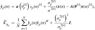
Given the estimate (14.72), the signal parameter ![]() can be obtained from (14.58) by replacing
can be obtained from (14.58) by replacing ![]() with
with ![]() , using
, using ![]() . Similarly, the noise parameter
. Similarly, the noise parameter ![]() is obtained from (14.59) by replacing
is obtained from (14.59) by replacing ![]() with
with ![]() .
.
The M-step (14.72) requires only a one dimensional search. The multi-dimensional nonlinear optimization in the original problem is greatly simplified by data augmentation. The EM algorithms for the known noise case [73,75] and the stochastic signal model [76] also demonstrate this computational advantage. A major shortcoming of EM is that it may converge slowly. To address this issue, we will discuss an implementation based on a more flexible augmentation scheme in the following.
To improve the convergence rate, the space alternating generalized EM (SAGE) algorithm [77] is derived in [78,79].
3.14.5.2.2 SAGE algorithm
The space alternating generalized EM (SAGE) algorithm [77] generalizes the idea of data augmentation to simplify computations of the EM algorithm. Instead of estimating all parameters at once, SAGE breaks up the problem into several smaller problems by conditioning sequentially on a subset of the parameters and then applies EM to each reduced problem. Because each of the reduced problems considers the likelihood as a function of a different subset of parameters, it is natural to use a different augmentation scheme for each of the corresponding EM algorithms [77,80]. In some settings, this attempt turns out to be very useful for speeding up the algorithm.
Unlike the EM algorithm, each iteration of SAGE consists of several cycles. The parameter subset associated with the cth cycle ![]() is updated by maximizing the conditional expectation of log-likelihood
is updated by maximizing the conditional expectation of log-likelihood ![]() of the augmented data
of the augmented data ![]() . The data augmentation schemes are allowed to vary between cycles. Within one iteration, every element of the parameter vector
. The data augmentation schemes are allowed to vary between cycles. Within one iteration, every element of the parameter vector ![]() must be updated at least once. Let
must be updated at least once. Let ![]() be the vector containing all parameters of
be the vector containing all parameters of ![]() except the elements of
except the elements of ![]() . Then
. Then ![]() is a partition of the parameter set at the cth cycle. The estimate at the cth cycle, ith iteration is represented by
is a partition of the parameter set at the cth cycle. The estimate at the cth cycle, ith iteration is represented by ![]() . The output of the last cycle of the ith iteration is used as the input of the
. The output of the last cycle of the ith iteration is used as the input of the ![]() st iteration:
st iteration: ![]() . Starting from the initial estimate
. Starting from the initial estimate ![]() , the
, the ![]() st iteration of the SAGE algorithm proceeds as follows. For
st iteration of the SAGE algorithm proceeds as follows. For ![]()
Similarly to EM, it can be shown that any sequence generated by the above procedure increases (or maintains) ![]() at every cycle [77].
at every cycle [77].
A natural augmentation scheme for DOA estimation is to consider one source at each cycle:
![]() (14.76)
(14.76)
Compared to the augmentation scheme specified in (14.71), ![]() is more noisy since the whole noise component is fully incorporated in every cycle. The parameter vector associated with the cth cycle is given by
is more noisy since the whole noise component is fully incorporated in every cycle. The parameter vector associated with the cth cycle is given by ![]() . The cth cycle in the
. The cth cycle in the ![]() st iteration is as follows:
st iteration is as follows:

The computational complexity for each iteration of EM and SAGE is almost the same. The total computational cost is determined by the convergence rate. It has been shown in [74] that the SAGE algorithm converges faster than the EM algorithm when certain conditions on observed and augmented information matrices are satisfied.
3.14.5.2.3 Iterative quadratic maximum likelihood
The iterative quadratic maximum likelihood (IQML) algorithm [81], also proposed independently in [82], can trace its root back to system identification methods [83]. Unlike EM and SAGE which are applicable to arbitrary arrays, the IQML algorithm requires a ULA so that the array response matrix ![]() has a Vandermonde structure:
has a Vandermonde structure:
 (14.80)
where ![]() according to (14.15). To re-parameterize the likelihood function (14.60), one defines a polynomial with roots
according to (14.15). To re-parameterize the likelihood function (14.60), one defines a polynomial with roots ![]() as
as
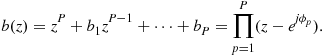 (14.81)
By construction, the Toeplitz matrix ![]()
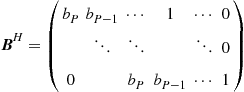 (14.82)
is full rank and satisfies the following relation:
![]() (14.83)
(14.83)
In other words, the column space of ![]() is orthogonal to that of
is orthogonal to that of ![]() . Therefore, the projection matrix in (14.60) can be reformulated as
. Therefore, the projection matrix in (14.60) can be reformulated as
![]() (14.84)
(14.84)
Then the likelihood criterion (14.60) can be re-parameterized in terms of the polynomial coefficients ![]()
![]() (14.85)
(14.85)
Maximizing ![]() leads to an estimate for the coefficient vector
leads to an estimate for the coefficient vector ![]() . With
. With ![]() replaced by
replaced by ![]() , the DOA estimate is computed by finding the roots of (14.81).
, the DOA estimate is computed by finding the roots of (14.81).
Minimization of the criterion (14.85) is still a complicated optimization problem. However, if the matrix ![]() is replaced by a known matrix, the criterion becomes quadratic in
is replaced by a known matrix, the criterion becomes quadratic in ![]() and has a closed form solution. This observation leads to the iterative algorithm suggested in [81]. Setting the initial value
and has a closed form solution. This observation leads to the iterative algorithm suggested in [81]. Setting the initial value ![]() and denoting the ith iterate as
and denoting the ith iterate as ![]() , the
, the ![]() st iteration of the IQML algorithm proceeds as follows:
st iteration of the IQML algorithm proceeds as follows:
![]() (14.86)
(14.86)
The procedure continues until the distance between two consecutive iterates is less than a pre-specified small number ![]() , i.e.,
, i.e., ![]() . To ensure the roots of the polynomial with estimated coefficients lie on the unit circle, constraints on
. To ensure the roots of the polynomial with estimated coefficients lie on the unit circle, constraints on ![]() have been suggested in [81,84]. For example, since
have been suggested in [81,84]. For example, since ![]() has all its roots on the unit circle, its coefficients satisfy the conjugate symmetry constraint:
has all its roots on the unit circle, its coefficients satisfy the conjugate symmetry constraint: ![]() . Similar to EM and SAGE, the IQML algorithm converges to local maxima which may or may not coincide with global optimal solution. The complexity of IQML algorithm is discussed in [85]. The asymptotic performance is investigated in [86]. In [87] an efficient implementation is suggested for the IQML algorithm.
. Similar to EM and SAGE, the IQML algorithm converges to local maxima which may or may not coincide with global optimal solution. The complexity of IQML algorithm is discussed in [85]. The asymptotic performance is investigated in [86]. In [87] an efficient implementation is suggested for the IQML algorithm.
3.14.5.3 Subspace fitting methods
The maximum likelihood approach exploits the parametric model and statistical distribution of array observations fully and exhibits excellent performance. The subspace fitting method [88–90] provides a unified framework for the deterministic ML estimator and subspace based methods. More specifically, it uses a nonlinear least square formulation
![]() (14.87)
(14.87)
where ![]() is a data matrix and
is a data matrix and ![]() is any matrix of conformable dimension. For fixed
is any matrix of conformable dimension. For fixed ![]() , the minimization with respect with
, the minimization with respect with ![]() measures how well the column spaces of
measures how well the column spaces of ![]() and
and ![]() match. Replacing the closed form solution
match. Replacing the closed form solution ![]() back into (14.87) results in a concentrated criterion:
back into (14.87) results in a concentrated criterion:
![]() (14.88)
(14.88)
Clearly, the deterministic ML estimator (14.61) can be obtained by using array observations as the data matrix ![]() .
.
The subspace fitting criterion is derived when the estimated signal eigenvectors are inserted as data ![]() . The weighted least square fitting solution to (14.87) has the expression:
. The weighted least square fitting solution to (14.87) has the expression:
![]() (14.89)
(14.89)
where the weighting matrix ![]() is Hermitian and positive definite. The analysis in [89,90] shows that the estimator
is Hermitian and positive definite. The analysis in [89,90] shows that the estimator ![]() is strongly consistent and asymptotically normally distributed. Minimization of the error covariance matrix of
is strongly consistent and asymptotically normally distributed. Minimization of the error covariance matrix of ![]() leads to the optimal weighting matrix
leads to the optimal weighting matrix ![]() where
where ![]() . Recall that the diagonal matrix
. Recall that the diagonal matrix ![]() contains P signal eigenvalues and
contains P signal eigenvalues and ![]() denotes the noise eigenvalue. In practice, both
denotes the noise eigenvalue. In practice, both ![]() and
and ![]() are estimated from data. The weighted subspace fitting (WSF) algorithm (or the method of direction estimation (MODE) [91]) is obtained when a consistent estimator
are estimated from data. The weighted subspace fitting (WSF) algorithm (or the method of direction estimation (MODE) [91]) is obtained when a consistent estimator ![]() is inserted into (14.89):
is inserted into (14.89):
![]() (14.90)
(14.90)
The signal subspace fitting formulation (14.89) has certain advantages over the data-domain nonlinear least square (14.87), in particular when ![]() . It is then significantly cheaper to compute (14.89) than (14.87).
. It is then significantly cheaper to compute (14.89) than (14.87).
In addition to the criterion (14.89), a noise subspace fitting formulation is developed in [91]. Although the resulting criterion is quadratic in the steering matrix ![]() , the noise subspace fitting criterion can not produce reliable estimates in the presence of signal coherence. The covariance matching estimator [92] that will be presented shortly can be formulated as (14.87).
, the noise subspace fitting criterion can not produce reliable estimates in the presence of signal coherence. The covariance matching estimator [92] that will be presented shortly can be formulated as (14.87).
The implementation of nonlinear least square type criteria (14.87) has been addressed in several papers [64,77,93]. A common feature of these methods is similar to the SAGE algorithm in the sense that instead of maximizing all parameters simultaneously, a subset of parameters, or the parameters associated with one signal source is computed in one step while keeping other parameters fixed. The RELAX procedure [93] is similar to the SAGE algorithm (14.77) and (14.79), although it has a simpler motivation and interpretation. The WSF (or MODE) criterion (14.90) can be formulated in terms of polynomial coefficients for ULAs by the expression (14.84) [91]. An iterative implementation, iterative MODE, similar to IQML is suggested in [84]. Theoretical and numerical results in [84] show that iterative MODE provides more accurate estimates and is computationally more efficient than IQML.
3.14.5.4 Covariance matching estimation methods
The covariance matching estimation methods are referred to as generalized least squares in the statistical literature. The application to array processing has led to several interesting algorithms [92,94–97]. Covariance matching can treat temporally correlated data and provides the same large sample properties as maximum likelihood estimation at often a lower computational cost [92].
Recall that the array output covariance matrix is give by ![]() . By stacking the columns of
. By stacking the columns of ![]() , one obtains the following expression:
, one obtains the following expression:
 (14.91)
where the elements of ![]() are source signal covariance parameters,
are source signal covariance parameters, ![]() is a known matrix, and
is a known matrix, and ![]() is a given function of the unknown parameter vector
is a given function of the unknown parameter vector ![]() . In general, the DOA parameter vector
. In general, the DOA parameter vector ![]() enters
enters ![]() in a nonlinear fashion. An estimate for
in a nonlinear fashion. An estimate for ![]() can be obtained from the sample covariance matrix by
can be obtained from the sample covariance matrix by ![]() . Fitting the data
. Fitting the data ![]() to the model (14.91) in the weighted least squares sense leads to the following criterion
to the model (14.91) in the weighted least squares sense leads to the following criterion
![]() (14.92)
(14.92)
where the weighting matrix ![]() is a consistent estimate of the covariance matrix
is a consistent estimate of the covariance matrix ![]() . The symbol
. The symbol ![]() denotes the Kronecker matrix product.
denotes the Kronecker matrix product.
The least square criterion is separable in the linear and nonlinear parameters. Minimizing (14.92) over the linear parameter vector ![]() results in a closed form expression:
results in a closed form expression:
![]() (14.93)
(14.93)
Substituting (14.93) into (14.92) leads to a concentrated criterion:
![]() (14.94)
(14.94)
where ![]() denotes a projection matrix onto the column space of
denotes a projection matrix onto the column space of ![]() . To apply (14.94), one needs to find the matrix
. To apply (14.94), one needs to find the matrix ![]() corresponding to the covariance matrix of the array observations. Based on the extended invariance principle, it was shown that the covariance matching estimator is a large sample realization of the ML method and asymptotically efficient [92]. A drawback of the covariance matrix matching based estimation methods is that they inherently assume a large sample size, and are less suitable to scenarios involving a small number of observations and high SNRs.
corresponding to the covariance matrix of the array observations. Based on the extended invariance principle, it was shown that the covariance matching estimator is a large sample realization of the ML method and asymptotically efficient [92]. A drawback of the covariance matrix matching based estimation methods is that they inherently assume a large sample size, and are less suitable to scenarios involving a small number of observations and high SNRs.
3.14.5.5 Performance bound
The performance of an estimator is measured by its average distance to the true parameters. In many cases, one is interested in the following questions: (1) Whether it converges to the true parameter as the number of data samples approaches infinity. (2) Whether the asymptotic error covariance matrix attains the Cramér-Rao bound (CRB). These two properties, consistency and efficiency, and the error covariance matrix are major concerns in a performance study. In this section, we will outline several important results. A comprehensive coverage on performance analysis is given in Chapter 14 in this book.
It is well known that the estimation error covariance of any unbiased estimator is lower bounded by the Cramér-Rao bound [54]. The Crámer-Rao bounds for the conditional and unconditional model are derived in [98–100], respectively. The conditional CRB, denoted by ![]() is given by
is given by
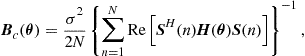 (14.95)
where ![]() contains the first derivative of steering vectors,
contains the first derivative of steering vectors, ![]() , and
, and ![]() . For
. For ![]() , the conditional CRB tends to the limit
, the conditional CRB tends to the limit
![]() (14.96)
(14.96)
The unconditional CRB, denoted by ![]() , is given by
, is given by
![]() (14.97)
(14.97)
From (14.95) and (14.97), we can observe that the CRBs decrease with increasing number of snapshots. Theoretical analysis and simulation results also show that the CRBs decrease as the number of sensors or SNRs grow.
3.14.5.5.1 ML methods
The CRBs (14.95) and (14.97) are related as ![]() in a positive definite sense. Because the number of signal parameters
in a positive definite sense. Because the number of signal parameters ![]() increases with the number of snapshots, the conditional CRB can not be attained by the conditional ML estimator. Under the unconditional data model, the parameter vector remains finite dimensional when
increases with the number of snapshots, the conditional CRB can not be attained by the conditional ML estimator. Under the unconditional data model, the parameter vector remains finite dimensional when ![]() , the unconditional ML estimator is consistent and achieves the unconditional CRB asymptotically. Let
, the unconditional ML estimator is consistent and achieves the unconditional CRB asymptotically. Let ![]() and
and ![]() denote the covariance matrix of the conditional and unconditional ML estimators, respectively. The following inequality is proved in [100]:
denote the covariance matrix of the conditional and unconditional ML estimators, respectively. The following inequality is proved in [100]: ![]() . In summary, the conditional ML estimator is consistent, but not efficient; whereas the unconditional ML estimator is both consistent and efficient.
. In summary, the conditional ML estimator is consistent, but not efficient; whereas the unconditional ML estimator is both consistent and efficient.
3.14.5.5.2 Subspace methods
The subspace methods are derived from signal—and noise eigenvector/eigenvalue estimates. Therefore, statistical properties of the eigen-analysis of ![]() [8] play an important role in the performance study. The asymptotic distribution derived in [98] shows that the MUSIC algorithm is a consistent estimator. Its covariance matrix may grow rapidly when some of the signal eigenvalues are close to the noise eigenvalue. This scenario occurs when two signals are closely located or correlated, leading to an almost rank deficient
[8] play an important role in the performance study. The asymptotic distribution derived in [98] shows that the MUSIC algorithm is a consistent estimator. Its covariance matrix may grow rapidly when some of the signal eigenvalues are close to the noise eigenvalue. This scenario occurs when two signals are closely located or correlated, leading to an almost rank deficient ![]() . For uncorrelated signals, the MUSIC estimator exhibits good performance comparable with the conditional ML estimator. The asymptotic performance of MUSIC is investigated in [101]. A performance study of root-MUSIC can be found in [36,37]. Asymptotic analysis of ESPRIT is carried out in [90,102].
. For uncorrelated signals, the MUSIC estimator exhibits good performance comparable with the conditional ML estimator. The asymptotic performance of MUSIC is investigated in [101]. A performance study of root-MUSIC can be found in [36,37]. Asymptotic analysis of ESPRIT is carried out in [90,102].
3.14.5.6 Numerical examples
In this section, we compare the performance of conditional ML estimator and root-MUSIC algorithm in a simulated environment. A ULA of 12 elements with half wavelength spacing is employed to receive two far-field narrow band signal sources of equal strengths located at ![]() . The sample covariance matrix is estimated from
. The sample covariance matrix is estimated from ![]() snapshots. Each experiment performs 500 Monte Carlo trials.
snapshots. Each experiment performs 500 Monte Carlo trials.
The RMSEs for DOA estimates and the conditional CRB (14.95) for uncorrelated and correlated signals are depicted in Figures 14.8 and 14.9, respectively. For the uncorrelated case, ML performs slightly better than root-MUSIC; in particular, at low SNR between −5 and 5 dB. In the correlated case with the correlation coefficient ![]() , while the deterministic ML estimator performs as well as in the uncorrelated case and close to the CRB, root-MUSIC no longer provides reliable estimates. As can be observed from Figure 14.9, even for SNR as high as 10 dB, root-MUSIC has RMSE larger than
, while the deterministic ML estimator performs as well as in the uncorrelated case and close to the CRB, root-MUSIC no longer provides reliable estimates. As can be observed from Figure 14.9, even for SNR as high as 10 dB, root-MUSIC has RMSE larger than ![]() . The difference between ML and root-MUSIC is most significant at low SNRs. In other words, the ML estimator is more robust than root-MUSIC against signal correlation and low SNRs. Although the performance of root-MUSIC is improved by forward-backward averaging, the RMSE is still larger than the ML approach. For SNR below 0 dB, it is twice as much as that of ML.
. The difference between ML and root-MUSIC is most significant at low SNRs. In other words, the ML estimator is more robust than root-MUSIC against signal correlation and low SNRs. Although the performance of root-MUSIC is improved by forward-backward averaging, the RMSE is still larger than the ML approach. For SNR below 0 dB, it is twice as much as that of ML.

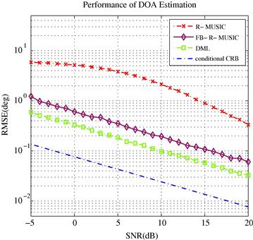
As mentioned previously, the ML estimator requires multi-dimensional nonlinear optimization. We compare three different implementations: (1) matlab function fmincon, (2) EM algorithm, (3) SAGE algorithm. The initial estimates for (1). are found by the genetic algorithm. The initial estimates for EM and SAGE are fixed at ![]() to simplify the investigation of their convergence behavior. Figure 14.10 shows that all three methods find ML estimates and achieve the same accuracy. To compare the convergence behavior of EM and SAGE, we plot the average log-likelihood value vs. iterations in Figure 14.11. As the convergence analysis in [74] predicted, SAGE converges faster than EM. It requires only 6 iterations to reach the final likelihood value, while EM requires 15 iterations. This is further confirmed by the average total number of iterations shown in Figure 14.12. As we can observe, at SNR from −10 dB to 5 dB, EM needs more than twice iterations than SAGE. For moderate to high SNR, the number of iterations of EM always exceeds that of SAGE by at least six iterations. This suggests that EM requires
to simplify the investigation of their convergence behavior. Figure 14.10 shows that all three methods find ML estimates and achieve the same accuracy. To compare the convergence behavior of EM and SAGE, we plot the average log-likelihood value vs. iterations in Figure 14.11. As the convergence analysis in [74] predicted, SAGE converges faster than EM. It requires only 6 iterations to reach the final likelihood value, while EM requires 15 iterations. This is further confirmed by the average total number of iterations shown in Figure 14.12. As we can observe, at SNR from −10 dB to 5 dB, EM needs more than twice iterations than SAGE. For moderate to high SNR, the number of iterations of EM always exceeds that of SAGE by at least six iterations. This suggests that EM requires ![]() more computational time than SAGE. It should be mentioned that the genetic algorithm [67] requires more than 10 times as long computational time compared to SAGE.
more computational time than SAGE. It should be mentioned that the genetic algorithm [67] requires more than 10 times as long computational time compared to SAGE.
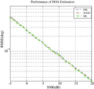
Figure 14.10 RMSE vs. SNR. EM, SAGE, ML with Newton methods. Uncorrelated signals. Reference DOA parameter ![]() ,
, ![]() ,
, ![]() .
.


3.14.6 Wideband DOA estimation
The DOA estimation methods presented previously are suitable for narrow band signals that often occur in communications and radar systems. In applications like sonar or seismic monitoring, the signals are often broadband. The important issue for the wideband case is how to combine multiple frequencies in an optimal way. For the maximum likelihood approach, the extension is straightforward because of the asymptotic properties of the Fourier transform [3,76,103]. Since the signal subspace is different for various frequencies, subspace methods require a pre-processing procedure to form a coherent averaging of the signal subspace as suggested in [104,105]. Another approach is to evaluate the spectral matrix and derive estimates from each frequency and then combine these estimates in some appropriate way [106]. Numerical results show that the former coherent approach provides better estimates than the latter one. In the following, we will describe the wideband version of the ML estimators and then discuss the coherent signal subspace method.
3.14.6.1 Wideband maximum likelihood estimation
In Section 3.14.2.2.1, the data model (14.10) was developed for a continuous temporal array output ![]() . In practice, the array outputs are temporally sampled at a properly chosen frequency. The data within an observation interval
. In practice, the array outputs are temporally sampled at a properly chosen frequency. The data within an observation interval ![]() is divided into K non-overlapping snapshots of length
is divided into K non-overlapping snapshots of length ![]() and Fourier-transformed. For large number of samples, the frequency domain data
and Fourier-transformed. For large number of samples, the frequency domain data ![]() can be modeled by (14.10). Under some regularity conditions including stationarity of array outputs, the following asymptotic properties hold [107]:
can be modeled by (14.10). Under some regularity conditions including stationarity of array outputs, the following asymptotic properties hold [107]:
1. ![]() are independent, identically complex normally distributed with zero mean and covariance matrix
are independent, identically complex normally distributed with zero mean and covariance matrix ![]() .
.
2. For ![]() are stochastically independent.
are stochastically independent.
3. Given the signal vector ![]() is complex normally distributed with mean
is complex normally distributed with mean ![]() and covariance matrix
and covariance matrix ![]() .
.
In the following, we assume that ![]() . Because of the independency between different frequency bins, the likelihood function is a product of those associated with various frequencies. For the deterministic data model, the log-likelihood function is given by
. Because of the independency between different frequency bins, the likelihood function is a product of those associated with various frequencies. For the deterministic data model, the log-likelihood function is given by
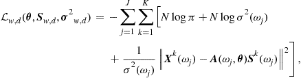 (14.98)
where the signal vector ![]() and noise vector
and noise vector ![]() contain signal and noise parameters of J frequencies. Similar to the narrow band case, the likelihood function can be concentrated with respect to the signal and noise parameters, leading to the concentrated likelihood function
contain signal and noise parameters of J frequencies. Similar to the narrow band case, the likelihood function can be concentrated with respect to the signal and noise parameters, leading to the concentrated likelihood function
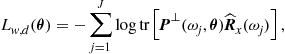 (14.99)
where the sample covariance matrix ![]() and
and ![]() is the orthogonal complement of the projection matrix
is the orthogonal complement of the projection matrix ![]() . Note that the summand in (14.99) has the same form as the narrow band likelihood function (14.61). The broadband criterion can be considered as an arithmetic average of narrow band likelihood functions over frequencies. The deterministic ML estimate is computed by maximizing this criterion or minimizing the negative log-likelihood:
. Note that the summand in (14.99) has the same form as the narrow band likelihood function (14.61). The broadband criterion can be considered as an arithmetic average of narrow band likelihood functions over frequencies. The deterministic ML estimate is computed by maximizing this criterion or minimizing the negative log-likelihood:
![]() (14.100)
(14.100)
For the stochastic signal model, the log-likelihood function is given by
 (14.101)
where ![]() contains signal spectral parameters of all frequencies and
contains signal spectral parameters of all frequencies and ![]() includes noise power parameters. Similar to the narrow band case, the stochastic likelihood function can be simplified by substituting ML estimates of signal and noise parameters into (14.101), leading to the concentrated criterion:
includes noise power parameters. Similar to the narrow band case, the stochastic likelihood function can be simplified by substituting ML estimates of signal and noise parameters into (14.101), leading to the concentrated criterion:
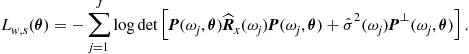 (14.102)
where ![]() is an estimate for the noise parameter. Similar to the deterministic case, (14.102) is an average of the narrow band likelihood criterion (14.61) over frequencies. The stochastic ML estimator is then obtained by maximizing this criterion or minimizing the negative likelihood:
is an estimate for the noise parameter. Similar to the deterministic case, (14.102) is an average of the narrow band likelihood criterion (14.61) over frequencies. The stochastic ML estimator is then obtained by maximizing this criterion or minimizing the negative likelihood:
![]() (14.103)
(14.103)
The performance analysis in [66] shows that under regularity conditions, ![]() is an asymptotically consistent, efficient estimator for
is an asymptotically consistent, efficient estimator for ![]() . The deterministic ML estimator
. The deterministic ML estimator ![]() is asymptotically consistent, but not efficient. The computation complexity can be also simplified by the EM or EM-like algorithms [74,76].
is asymptotically consistent, but not efficient. The computation complexity can be also simplified by the EM or EM-like algorithms [74,76].
3.14.6.2 Coherent signal subspace methods
The coherent signal subspace methods proposed in [105] combine the broadband data by multiplying each frequency with the focusing matrix ![]() satisfying the following property
satisfying the following property
![]() (14.104)
(14.104)
where ![]() is a selected reference frequency. The coherently averaged covariance matrix
is a selected reference frequency. The coherently averaged covariance matrix ![]() is given by
is given by
 (14.105)
where ![]() is the sum of noise level over frequencies and
is the sum of noise level over frequencies and ![]() . Given the known noise structure
. Given the known noise structure ![]() , the eigenvalue/eigenvector pairs of
, the eigenvalue/eigenvector pairs of ![]() satisfy the same properties (14.36), (14.37) as in the narrow band case. Hence, the subspace methods introduced previously can be applied to the new matrix (14.105).
satisfy the same properties (14.36), (14.37) as in the narrow band case. Hence, the subspace methods introduced previously can be applied to the new matrix (14.105).
The design of (14.104) requires a rough estimate of the DOA parameter, which can be obtained from the narrow band MVDR or conventional beamformer. In [104], the rotational signal subspace focusing matrix is developed by solving the constrained optimization problem:
![]() (14.106)
(14.106)
![]() (14.107)
(14.107)
The solution to (14.106) is given by ![]() , where the columns of
, where the columns of ![]() and
and ![]() are left and right singular vectors of
are left and right singular vectors of ![]() . The selection of reference frequency and accuracy improvement are discussed in detail in [104,105]. Within the class of signal subspace transformation matrices, the rotational subspace transformation matrix is well known for their optimality in preserving SNR after focusing [108]. In practice, the spatial correlation matrix
. The selection of reference frequency and accuracy improvement are discussed in detail in [104,105]. Within the class of signal subspace transformation matrices, the rotational subspace transformation matrix is well known for their optimality in preserving SNR after focusing [108]. In practice, the spatial correlation matrix ![]() is replaced by the sample covariance matrix
is replaced by the sample covariance matrix ![]() . By (14.105), we compute the coherently averaged sample covariance matrix
. By (14.105), we compute the coherently averaged sample covariance matrix ![]() and construct coherent signal/noise subspaces from
and construct coherent signal/noise subspaces from ![]() . Then standard subspace methods are applied with
. Then standard subspace methods are applied with ![]() as the reference frequency for DOA estimation.
as the reference frequency for DOA estimation.
In [109], coherent subspace averaging is achieved by using weighted signal subspaces ![]() instead of the array correlation matrix
instead of the array correlation matrix ![]() in (14.105), where
in (14.105), where ![]() contains signal eigenvectors at frequency
contains signal eigenvectors at frequency ![]() and
and ![]() is a weighting matrix. While the aforementioned methods concentrates on the design of the best coherently averaged signal subspaces and finding the DOA estimates by standard narrow band eigenstructure based algorithms such as MUSIC, the test of orthogonality of projected subspaces (TOPS) algorithm proposed in [110] utilizes the property of transformed signal subspaces and test whether the hypothesized subspaces and the noise subspaces are orthogonal. A significant advantage of this approach is that it does not require initial DOA estimates. Simulation results in [110] show that TOPS performs better than the aforementioned methods in mid SNR ranges, while the coherent methods work best at low SNR and incoherent methods work best at high SNR.
is a weighting matrix. While the aforementioned methods concentrates on the design of the best coherently averaged signal subspaces and finding the DOA estimates by standard narrow band eigenstructure based algorithms such as MUSIC, the test of orthogonality of projected subspaces (TOPS) algorithm proposed in [110] utilizes the property of transformed signal subspaces and test whether the hypothesized subspaces and the noise subspaces are orthogonal. A significant advantage of this approach is that it does not require initial DOA estimates. Simulation results in [110] show that TOPS performs better than the aforementioned methods in mid SNR ranges, while the coherent methods work best at low SNR and incoherent methods work best at high SNR.
3.14.7 Signal detection
Estimation of the number of signals is fundamental to array processing algorithms. It is usually the first step in the application of direction finding algorithms. In the previous discussion, we assumed that the number of signals, P, is known a priori. In practice, the number of signals needs to be estimated from measurements as well. Popular approaches for determining the number of signals can be classified as nonparametric or parametric methods. The former utilizes the eigenstructure of the array correlation matrix (14.13) and estimates the dimension of the signal subspace by employing the information theoretic criteria [10,111–113] or hypothesis tests [63,114,115]. Parametric methods exploit the array output model (14.12) and jointly estimate the parameter and number of signals [65,116–118]. The nonparametric approach is computationally simple but sensitive to signal coherence and small data samples. The parametric approach requires more time for parameter estimation, but performs significantly better than the nonparametric one in critical scenarios. In the following, we will describe the ideas behind the aforementioned methods briefly and give more related references.
3.14.7.1 Nonparametric methods
We have learned in subspace methods that the array correlation matrix (14.13) has the eigen-decomposition ![]() where the diagonal matrix
where the diagonal matrix ![]() consists of the P largest eigenvalues and
consists of the P largest eigenvalues and ![]() contains corresponding eigenvectors. The remaining
contains corresponding eigenvectors. The remaining ![]() eigenvalues/vectors are included in
eigenvalues/vectors are included in ![]() and
and ![]() in a similar way. When the signal covariance matrix
in a similar way. When the signal covariance matrix ![]() is full rank, the eigenvalues satisfy the property
is full rank, the eigenvalues satisfy the property
![]() (14.108)
(14.108)
The smallest ![]() noise eigenvalues are equal to
noise eigenvalues are equal to ![]() . This observation suggests that the number of signals can be determined from the multiplicity of the smallest eigenvalue. In practice, the correlation matrix
. This observation suggests that the number of signals can be determined from the multiplicity of the smallest eigenvalue. In practice, the correlation matrix ![]() is unknown and the eigenvalues are estimated from the sample covariance matrix
is unknown and the eigenvalues are estimated from the sample covariance matrix ![]() . The ordered sample eigenvalues
. The ordered sample eigenvalues ![]() are distinct with probability one [8].
are distinct with probability one [8].
The sphericity test, originating from the statistical literature [119], is modified for detection purpose in [115]. Therein, a series of nested hypothesis tests is formulated to test the equality of ![]() eigenvalues, i.e.,
eigenvalues, i.e.,
![]() (14.109)
(14.109)
![]()
where ![]() and
and ![]() denote the null hypothesis and alternative, respectively. Starting from
denote the null hypothesis and alternative, respectively. Starting from ![]() , the test proceeds to the next hypothesis if
, the test proceeds to the next hypothesis if ![]() is rejected. Upon acceptance of
is rejected. Upon acceptance of ![]() , the test stops, implying all remaining tests are true and leading to the estimate
, the test stops, implying all remaining tests are true and leading to the estimate ![]() . For non-Gaussian distribution and small samples case, the test statistic does not have a closed form expression for null distribution. To overcome this problem, a procedure using bootstrap techniques are developed in [114]. The test for unknown noise fields is suggested in [120]. Recently, due to the development of random matrix theory, the eigenvalue based multiple test is re-visited for the small sample case in [121,122] and the references therein.
. For non-Gaussian distribution and small samples case, the test statistic does not have a closed form expression for null distribution. To overcome this problem, a procedure using bootstrap techniques are developed in [114]. The test for unknown noise fields is suggested in [120]. Recently, due to the development of random matrix theory, the eigenvalue based multiple test is re-visited for the small sample case in [121,122] and the references therein.
The information theoretic criteria based approach views signal detection as model order selection. The Akaike’s information criterion (AIC) and Rissanen’s minimum description length (MDL) was derived for signal detection in [111]. In the derivation, the data set ![]() is parameterized by the eigenvalues and eigenvectors of correlation matrix
is parameterized by the eigenvalues and eigenvectors of correlation matrix ![]() , rather than the DOA parameter. Maximization of the log-likelihood function leads to the AIC criterion
, rather than the DOA parameter. Maximization of the log-likelihood function leads to the AIC criterion
 (14.110)
and the MDL criterion
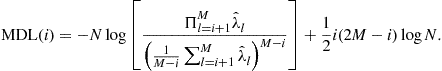 (14.111)
The number of signals ![]() is determined as the minimizing value
is determined as the minimizing value ![]() of AIC or MDL, where
of AIC or MDL, where ![]() denotes the maximal number of signals. Eqs. (14.110) and (14.111) show that both criteria has the first term in common, which is a ratio between geometric mean and arithmetic mean of the smallest
denotes the maximal number of signals. Eqs. (14.110) and (14.111) show that both criteria has the first term in common, which is a ratio between geometric mean and arithmetic mean of the smallest ![]() eigenvalues. The penalty term of AIC depends only on the number of free adjustable parameters, while the penalty term of MDL depends also on the data length N. In general, AIC tends to overestimate the number of signals while MDL is consistent as the number of samples approaches infinity [111,123]. Various improvement strategies for MDL for situations involving fully correlated signals, correlated noise and small samples have been suggested in [112,124–127] and references therein.
eigenvalues. The penalty term of AIC depends only on the number of free adjustable parameters, while the penalty term of MDL depends also on the data length N. In general, AIC tends to overestimate the number of signals while MDL is consistent as the number of samples approaches infinity [111,123]. Various improvement strategies for MDL for situations involving fully correlated signals, correlated noise and small samples have been suggested in [112,124–127] and references therein.
3.14.7.2 Parametric methods
In parametric methods, the DOA parameter in the model (14.12) enters the algorithms directly. Determination of the number of signals can be formulated as a multiple hypothesis test. In the multiple hypothesis test approach, we consider a series of nested hypotheses.
![]() (14.112)
(14.112)
The subscripts ![]() and i are used to emphasize the dimension of the steering matrix and the signal vector under the null hypothesis
and i are used to emphasize the dimension of the steering matrix and the signal vector under the null hypothesis ![]() and the alternative
and the alternative ![]() , respectively. Here, the signal vectors are considered as unknown and deterministic.
, respectively. Here, the signal vectors are considered as unknown and deterministic.
In [116,118,128], a sequential test procedure is developed to detect the signal one after another. Starting from noise only case, ![]() is tested against
is tested against ![]() . If
. If ![]() is rejected, a new signal is declared as detected and the test procedure proceeds to the next hypothesis
is rejected, a new signal is declared as detected and the test procedure proceeds to the next hypothesis ![]() . It stops when the null hypothesis is accepted, implying that no further signal can be detected. The number of signals is then estimated by the dimension of the signal vector under the accepted null hypothesis. The test statistics are constructed by the generalized likelihood ratio principle. In the narrow band case, it leads to an F-test similar to that suggested in [129]. For broadband data, a closed form expression for the null distribution is not available. In this case, bootstrap techniques or Edgeworth expansions can be applied to approximate the significance level or test threshold. The global significance level in the sequential test procedure is usually controlled by Bonferroni-type procedures. As each test is conducted at a much lower level, results may be conservative when the size of the problem increases. A more powerful test procedure based on the false discovery rate criterion is developed in [117]. A joint estimation and detection procedure was also investigated in [65].
. It stops when the null hypothesis is accepted, implying that no further signal can be detected. The number of signals is then estimated by the dimension of the signal vector under the accepted null hypothesis. The test statistics are constructed by the generalized likelihood ratio principle. In the narrow band case, it leads to an F-test similar to that suggested in [129]. For broadband data, a closed form expression for the null distribution is not available. In this case, bootstrap techniques or Edgeworth expansions can be applied to approximate the significance level or test threshold. The global significance level in the sequential test procedure is usually controlled by Bonferroni-type procedures. As each test is conducted at a much lower level, results may be conservative when the size of the problem increases. A more powerful test procedure based on the false discovery rate criterion is developed in [117]. A joint estimation and detection procedure was also investigated in [65].
Simulation shows that the multiple hypothesis approach has superior performance than information theoretic approach [117]. In particular, signal coherence has little impact on the performance. Due to ML estimates required in the test, parametric methods are computationally more expensive than eigenvalue based methods.
3.14.7.3 Additional issues
When the estimated number of signals, ![]() , provided by detection algorithms is accurate, the performance of DOA estimation is well studied in the literature. In the low SNR region and small sample case, the number of signals may be over- or underestimated. In the presence of overestimated signals, the true DOA parameters are included in the oversized parameter vector with increased variance for the true parameters. In the case of under estimation, the inaccuracy in signal numbers will lead to bias and increased mean squared errors [130]. Robust algorithms have been suggested in [131,132] to retrieve information when the number of signals is unknown.
, provided by detection algorithms is accurate, the performance of DOA estimation is well studied in the literature. In the low SNR region and small sample case, the number of signals may be over- or underestimated. In the presence of overestimated signals, the true DOA parameters are included in the oversized parameter vector with increased variance for the true parameters. In the case of under estimation, the inaccuracy in signal numbers will lead to bias and increased mean squared errors [130]. Robust algorithms have been suggested in [131,132] to retrieve information when the number of signals is unknown.
3.14.8 Special topics
We have presented DOA estimation algorithms assuming far-field propagation and static sources. In practice, these conditions may change and require modification to standard algorithms. In the following, we will discuss several interesting issues and provide related references.
3.14.8.1 Tracking
Localization of moving sources is essential to many applications. In the classical tracking problem, the DOA estimates obtained from array data are considered as input data for track estimation. The main task is to match DOA estimates and to contacts, and many solutions have been developed to solve the data association problem [133,134]. An alternative approach incorporates target motion into the likelihood function and estimates the DOA parameter, and velocity directly from data [135–137]. In [138,139], the EM algorithm is suggested to reduce the computational cost for maximizing the likelihood function. To further simplify the implementation, the recursive EM algorithm is developed in [128,140]. The recursive EM algorithm is a stochastic approximation procedure for finding ML estimates [141]. With a specialized gain matrix derived from the EM algorithm, it has a simple implementation and leads to asymptotic normality and consistency. With a proper formulation, it can also be used for estimating time varying DOA parameters.
For subspace methods, how to compute the time-varying signal or noise subspaces efficiently becomes the most important step. In early works, classical batch Eigenvalue Decomposition/SVD techniques have been modified for the use in adaptive processing. Fast computation methods based on subspace averaging were proposed in [142–144]. Another class of algorithms considers ED/SVD as a constrained or unconstrained optimization problem [145–149]. For example, in [149], it is shown that the signal subspace can be computed by solving the following unconstrained optimization problem:
![]() (14.113)
(14.113)
where ![]() denotes the matrix argument and r is the number of signal eigenvectors. The aim of subspace tracking is to compute
denotes the matrix argument and r is the number of signal eigenvectors. The aim of subspace tracking is to compute ![]() efficiently at the time instant n from the subspace estimate at time instant
efficiently at the time instant n from the subspace estimate at time instant ![]() . For time-varying subspaces, the expectation in (14.113) is replaced by an exponentially weighted sum of snapshots to ensure the samples in the distant past is down weighted. In addition to low computational complexity, fast convergence and numerical stability are also desired properties in the implementation of subspace tracking techniques. Once the subspace estimates are updated, the DOA estimates are computed by subspace methods presented previously.
. For time-varying subspaces, the expectation in (14.113) is replaced by an exponentially weighted sum of snapshots to ensure the samples in the distant past is down weighted. In addition to low computational complexity, fast convergence and numerical stability are also desired properties in the implementation of subspace tracking techniques. Once the subspace estimates are updated, the DOA estimates are computed by subspace methods presented previously.
3.14.8.2 Signals with known structures
In some applications, the source signals exhibit specific structures and can be exploited for DOA estimation. For example, in communication systems, modulated signals are characterized by cyclostationarity, which is referred to as being periodically correlated. This property allows estimation of DOAs of only those signals having specified cycle frequency. Also, the noise can have unknown spatial characteristics as long as it is cyclically independent from signals of interest. Several direction finding algorithms were suggested and analyzed in [150–154].
In standard array processing methods, array data are assumed to be Gaussian and completely characterized by second order statistics. In the presence of non-Gaussian signals, higher order statistics can be exploited to the advantage of Gaussian noise suppression and increased aperture [155–158]. A common feature of both types of methods is the requirement of large amount of data samples to achieve comparable results as standard algorithms.
3.14.8.3 Spatially correlated noise fields
Most existing array processing methods assume that the background noise is spatially white, i.e., the covariance matrix is proportional to the identity matrix. This assumption is often violated in practical situations [159]. If the noise covariance matrix is known or estimated from signal-free measurements, the data can be pre-whitened. In the absence of this knowledge, the quality of DOA estimates degrade dramatically at low SNR [160,161].
Methods that take small errors in the assumed noise covariance into account are proposed in [63,162,163]. These algorithms are not applicable when the noise covariance is completely unknown, unless SNR is very high. Another approach considers parametric noise models and estimates DOA and noise parameters simultaneously [56,164,165]. In this approach, the additional noise parameters require extra computational time and increase variances of DOA estimates. In [166–168], the effect of unknown correlated noise is alleviated by the covariance differencing technique. The instrumental variables based approach is proposed in [169,170]. This technique relies on the assumption that the emitter signals are temporally correlated with correlation time significantly longer than that of the noise. Other solutions include exploitation of prior knowledge of signals [171] or specific array configurations [172]. In [171], the signal waveform is expressed as a linear combination of known basis functions. This assumption is reasonable in applications like radar and active sonar. The algorithm developed therein is a good example showing that knowledge of the spatially colored noise can be traded against alternative a priori information about signals.
3.14.8.4 Beamspace processing
The computational complexity for DOA estimation grows rapidly with data dimension, i.e., the number of sensors. In many applications like radar, arrays may have thousands of elements [4,173]. Methods for reducing the data dimension without loss of information are important to these scenarios. Motivated by the idea of beamforming, the beamspace processing employs a linear transformation to the outputs of the full sensors of the array
![]() (14.114)
(14.114)
where ![]() is an orthonormal
is an orthonormal ![]() transformation matrix. The columns of
transformation matrix. The columns of ![]() correspond to beamformers within a narrow DOA sector. The design of the transformation matrix is achieved by maximizing the average signal-to-noise ratio [174], selection of spatial sector [175] or minimizing error variances [176]. The beamspace processing may improve estimation performance by filtering out interferences outside the sector of interest and relax the assumption of white noise to local whiteness. As indicated in [177,178], the resolution threshold of the MUSIC algorithm can be lowered in beamspace. With prior knowledge on the true DOA parameter, it is possible to theoretically attain the Crámer-Rao bound by proper choice of the transformation matrix [176].
correspond to beamformers within a narrow DOA sector. The design of the transformation matrix is achieved by maximizing the average signal-to-noise ratio [174], selection of spatial sector [175] or minimizing error variances [176]. The beamspace processing may improve estimation performance by filtering out interferences outside the sector of interest and relax the assumption of white noise to local whiteness. As indicated in [177,178], the resolution threshold of the MUSIC algorithm can be lowered in beamspace. With prior knowledge on the true DOA parameter, it is possible to theoretically attain the Crámer-Rao bound by proper choice of the transformation matrix [176].
The adoption of beamspace processing into MUSIC and ESPRIT algorithms is addressed in [179] and references therein. It is interesting to observe that the array response vector becomes ![]() after the transformation (14.114). This allows a simpler expression of array manifold vector and facilitates the application of root-MUSIC and ESPRIT in the 2D case [180]. As pointed out in [180], beamspace transformation has a close link to array interpolation. The interpolated array scheme proposed by Friedlander and Weiss [38] employs a linear transformation to map the manifold vectors for an arbitrary array onto ULA-type response vectors. The field of view of the array is divided into L sectors, defined by
after the transformation (14.114). This allows a simpler expression of array manifold vector and facilitates the application of root-MUSIC and ESPRIT in the 2D case [180]. As pointed out in [180], beamspace transformation has a close link to array interpolation. The interpolated array scheme proposed by Friedlander and Weiss [38] employs a linear transformation to map the manifold vectors for an arbitrary array onto ULA-type response vectors. The field of view of the array is divided into L sectors, defined by ![]() . Then a set of angles is selected for each sector,
. Then a set of angles is selected for each sector,
![]() (14.115)
(14.115)
Let ![]() and
and ![]() denote the array response matrix of the real array and the virtual array with desired response, respectively. An interpolation matrix is computed for each sector as the least square solution such that
denote the array response matrix of the real array and the virtual array with desired response, respectively. An interpolation matrix is computed for each sector as the least square solution such that ![]() is minimized. One may use a weighted least square formulation to improve interpolation accuracy. In [181], an MSE design criterion is suggested to reduce DOA estimation bias caused by array interpolation. An interesting observation is the duality between array interpolation and coherent signal space averaging introduced in Section 3.14.6.2. The former designs the mapping matrix based on the spatially sampled frequencies, while the latter based on samples in the temporal frequency domain. Both techniques are useful for increasing applicability of computationally efficient subspace methods.
is minimized. One may use a weighted least square formulation to improve interpolation accuracy. In [181], an MSE design criterion is suggested to reduce DOA estimation bias caused by array interpolation. An interesting observation is the duality between array interpolation and coherent signal space averaging introduced in Section 3.14.6.2. The former designs the mapping matrix based on the spatially sampled frequencies, while the latter based on samples in the temporal frequency domain. Both techniques are useful for increasing applicability of computationally efficient subspace methods.
3.14.8.5 Distributed sources
In several array processing applications, such as radio communications, underwater acoustics and radar, physical measurements show that the effects of angle spread should be taken into account in the modeling. This appears in wireless communications, for example, an elevated base station experiences the received signal as distributed in space due to local scattering around the mobile [182,183]. The array output in distributed source modeling can be expressed as ![]() , where
, where ![]() describes the contribution of the ith signal to the array output. Unlike in the point source modeling where
describes the contribution of the ith signal to the array output. Unlike in the point source modeling where ![]() , the source energy is spread over some angular volume and is written as [184–186]
, the source energy is spread over some angular volume and is written as [184–186]
![]() (14.116)
(14.116)
where ![]() is the angular signal density of the ith source,
is the angular signal density of the ith source, ![]() contains location parameters of the ith source and
contains location parameters of the ith source and ![]() is the angular field of view. Examples for
is the angular field of view. Examples for ![]() are the two bounds of a uniformly distributed source or mean and standard deviation of source with Gaussian angular distribution. The problem of interest here is to estimate the unknown parameter vector
are the two bounds of a uniformly distributed source or mean and standard deviation of source with Gaussian angular distribution. The problem of interest here is to estimate the unknown parameter vector ![]() .
.
For small angular spread, the distributed source modeling (14.116) usually leads to a signal covariance matrix of the form
![]() (14.117)
(14.117)
where the matrix ![]() is a fully occupied matrix with elements depending on the array shape and signal distribution. As a result, the rank of the signal covariance matrix
is a fully occupied matrix with elements depending on the array shape and signal distribution. As a result, the rank of the signal covariance matrix ![]() is equal to the number of sensors M. This implies that a separation between signal subspace and noise subspace is not possible. To overcome this difficulty, a number of approaches based on subspace methods have been suggested. In [187], the signal subspace is approximated by eigenvectors associated with dominant eigenvalues. In [185,186], a generalized subspace in Hilbert space is defined to preserve the eigenstructure as in the point source modeling. Based on an approximation of the signal covariance matrix, a root-MUSIC algorithm is derived in [188]. In [189], the property of the inverse of the covariance matrix is exploited to establish the orthogonality between signal and noise subspace. Performance bounds and analysis of subspace methods in the context of distributed sources are considered in [190,191].
is equal to the number of sensors M. This implies that a separation between signal subspace and noise subspace is not possible. To overcome this difficulty, a number of approaches based on subspace methods have been suggested. In [187], the signal subspace is approximated by eigenvectors associated with dominant eigenvalues. In [185,186], a generalized subspace in Hilbert space is defined to preserve the eigenstructure as in the point source modeling. Based on an approximation of the signal covariance matrix, a root-MUSIC algorithm is derived in [188]. In [189], the property of the inverse of the covariance matrix is exploited to establish the orthogonality between signal and noise subspace. Performance bounds and analysis of subspace methods in the context of distributed sources are considered in [190,191].
Note that the distributed source modeling also affects the design of the adaptive beamformer as the distortionless constraint (14.27) no longer holds. In [185], a generalized minimum variance beamformer is proposed by considering total distributed energy of the signal. The resolution of [185] is found superior to [186–188] in simulation. While the above mentioned methods are mostly semiparametric, parametric methods based on ML approach and covariance matching techniques are derived in [97] and [94], respectively. Through the application of the extended invariance principle, the high computational complexity often encountered by the parametric approach is significantly lowered in [94].
3.14.8.6 Polarization sensitivity
Most direction finding algorithms presented before consider sensor arrays in which the output of each sensor is a scalar response to, for example, acoustic pressure or one component of the electric or magnetic fields. As the array manifold depends only on the direction of arrival, one is able to retrieve the spatial signature of the emitting signals without estimating polarization parameters. Polarization is an important property of electromagnetic waves. In wireless communications, polarization diversity has played a key in antenna design [192]. The transverse components of the electric or magnetic fields are related through polarization parameters. Due to this additional information, the DOA estimation performance can be improved by polarization sensitive antenna arrays. In [193], an extension of MUSIC is suggested for polarization sensitive arrays. The subspace fitting method, ML based approach and ESPRIT algorithm were developed for diversely polarized signals [61,194–199], respectively. A performance study can be found in [200,201].
A complete data model for vector sensors that characterizes all six components of the electromagnetic fields is suggested in [202]. Therein, it is shown that in contrast to scalar sensor arrays, DOA estimation is possible using only one single vector sensor. Identifiability and uniqueness issues related to vector sensors have been investigated in [203,204]. Other interesting applications including seismic localization, acoustics, and biomedical engineering have been discussed in [205–208].
3.14.9 Discussion
The problem of estimating the direction of arrival using an array of sensors has been discussed in detail in this contribution. Starting with the beamforming approach, we have presented eigenstructure based subspace methods and parametric methods. The spectral analysis based beamforming techniques are essentially spatial filters and requires least computational effort. Subspace methods achieve high resolution and estimation accuracy at an affordable computational cost. Parametric methods exploit the data model fully, and are characterized by excellent statistical properties and robustness in critical scenarios at the expense of increased computations. Selection of suitable algorithms depends on the underlying propagation environment, required accuracy and processing speed, available software and hardware. For simplicity, the essential DOA estimators are presented in the context of narrow band data. Techniques for processing broadband data are treated separately. Methods for signal detection are included in a separate section. Despite the richness of theoretical and experimental results in array processing, technological innovation and theoretical advances have shifted the research focus to application specific methods. To reflect this trend, we selected several topics including tracking, structured signals, correlated noise field, beamspace processing, distributed sources, and vector sensors for discussion.
The materials covered in this article are presented in a tutorial style, trying to serve the first exposure and as a tour guide into this exciting area. References listed here are by no means complete, but in the hope to assist interested readers for further study. More specialized aspects of array processing will be treated in detail by other contributing authors of this series. Their works are particularly valuable to fill the gap between this rather introductory review and in-depth knowledge. Finally, we feel extremely grateful to all researchers that have enriched the area of array processing and made this article possible.
Relevant Theory: Statistical Signal Processing and Signal Processing
• See Vol. 1, Chapter 4 Random Signals and Stochastic Processes
• See Vol. 1, Chapter 11 Parametric Estimation
• See this Volume, Chapter 2 Model Order Selection
• See this Volume, Chapter 8 Performance Analysis and Bounds
References
1. Capon J. High resolution frequency wave number spectrum analysis. Proc IEEE. 1969;57:1408–1418.
2. Schmidt RO. Multiple emitter location and signal parameter estimation. IEEE Trans Antennas Propag. 1986;34(3):276–280.
3. Böhme JF. Array processing. In: Haykin S, ed. Advances in Spectrum Analysis and Array Processing. Englewood Cliffs, NJ: Prentice Hall; 1991;1–63.
4. Krim H, Viberg M. Two decades of array signal processing research: the parametric approach. IEEE Signal Process Mag. 1996;13(4):67–94.
5. Van Veen BD, Buckley KM. Beamforming: a versatile approach to spatial filtering. IEEE Acoust Speech Signal Process Mag. 1988;4–24.
6. Johnson DH, Dugeon DE. Array Signal Processing: Concepts and Techniques. Prentice Hall 1993.
7. Van Trees HL. Optimum Array Processing (Detection, Estimation, and Modulation Theory, Part IV). New York: Wiley; 2002.
8. Anderson TW. An Introduction to Multivariate Statistical Analysis. third ed. Wiley 2003.
9. Bresler Y, Macovski A. On the number of signals resolvable by a uniform linear array. IEEE Trans Acoust Speech Signal Process ASSP-34 1986;1361–1375.
10. Wax M, Ziskind I. On unique localization of multiple sources by passive sensor arrays. IEEE Trans Acoust Speech Signal Process. 1989;37(7):996–1000.
11. R.T. Lacoss, Data adaptive spectral analysis methods, Geophysics 36 (71) 661–675.
12. Li J, Stoica P, Wang Z. On robust Capon beamforming and diagonal loading. IEEE Trans Signal Process. 2003;51(7):1702–1715.
13. Borgiotti G, Kaplan L. Superresolution of uncorrelated intereference sources by using adaptive array techniques. IEEE Trans Antennas Propag. 1979;27(3):842–845.
14. Huang M-X, Shih JJ, Lee RR, et al. Commonalities and differences among vectorized beamformers in electromagnetic source imaging. Brain Topogr. 2004;16:139–158.
15. Vaidyanathan C, Buckley KM. Performance analysis of the MVDR spatial spectrum estimator. IEEE Trans Signal Process. 1995;43(6):1427–1437.
16. Luthra A. A solution to the adaptive nulling problem with a look-direction constraint in the presence of coherent jammers. IEEE Trans Antennas Propag. 1986;34(5):702–710.
17. Owsley NL. An overview of optimum adaptive control in sonar array processing. In: Nardendra KS, Monopoli RV, eds. Applications of Adaptive Control. NewYork: Academic Press; 1980;131–164.
18. Reddy V, Paulraj A, Kailath T. Performance analysis of the optimum beamformer in the presence of correlated sources and its behavior under spatial smoothing. IEEE Trans Acoust Speech Signal Process. 1987;35(7):927–936.
19. Shan TJ, Kailath T. Adaptive beamforming for coherent signals and interference. IEEE Trans Acoust Speech Signal Process. 1985;33(3):527–536.
20. Tsai C-J, Yang J-F, Shiu T-H. Performance analyses of beamformers using effective SINR on array parameters. IEEE Trans Signal Process. 1995;43(1):300–303.
21. Zoltowski MD. On the performance analysis of the MVDR beamformer in the presence of correlated interference. IEEE Trans Acoust Speech Signal Process. 1988;36(6):945–947.
22. Richmond CD. Response of sample covariance based MVDR beamformer to imperfect look and inhomogeneities. IEEE Signal Process Lett. 1998;5(12):325–327.
23. Vorobyov SA, Gershman AB, Luo Z-Q. Robust adaptive beamforming using worst-case performance optimization: a solution to the signal mismatch problem. IEEE Trans Signal Process. 2003;51(2):313–324.
24. Fuchs J-J. On the application of the global matched filter to DOA estimation with uniform circular arrays. IEEE Trans Signal Process. 2001;49(4):702–709.
25. Malioutov D, Cetin M, Willsky AS. A sparse signal reconstruction perspective for source localization with sensor arrays. IEEE Trans Signal Process. 2005;53(8):3010–3022.
26. Tropp JA. Just relax: convex programming methods for identifying sparse signals in noise. IEEE Trans Info Theory. 2006;52(3):1030–1051.
27. Hyder MM, Mahata K. Direction-of-arrival estimation using a mixed ![]() norm approximation. IEEE Trans Signal Process. 2010;58(9):4646–4655.
norm approximation. IEEE Trans Signal Process. 2010;58(9):4646–4655.
28. Yin J, Chen T. Direction-of-arrival estimation using a sparse representation of array covariance vectors. IEEE Trans Signal Process. 2011;59(9):4489–4493.
29. Panahi A, Viberg M. On the resolution of the Lasso-based Doa estimation method. In: International ITG Workshop on Smart Antennas (WSA 2011), Aachen, Germany. IEEE 2011.
30. Pisarenko VF. The retrieval of harmonics from a covariance function. Geophys J Roy Astron Soc. 1973;33:347–366.
31. Bienvenu G, Kopp L. Principle de la goniometrie passive adaptive. In: Proceedings of the 7’eme Colloque GRESIT, Nice, France. 1979;106/1–106/10.
32. Schmidt RO. Multiple emitter location and signal parameter estimation. In: Proceedings of the RADC Spectrum Estimation Workshop, Rome, NY. 1979;243–258.
33. Oh SK, Un CK. A sequential estimation approach for performance improvement of eigen-structure based methods in array processing. IEEE Trans Signal Process. 1993;1(41):457–463.
34. Stoica P, Handel P, Nehoral A. Improved sequential MUSIC. IEEE Trans Aerosp Electron Syst. 1995;31(4):1230–1239.
35. Kung SY, Arun KS, Bhaskar Rao DV. State-space and singular-value decomposition-based approximation methods for the harmonic retrieval problem. J Opt Soc Am. 1983;73(12):1799–1811.
36. Barabell AJ. Improving the resolution performance of eigenstructure-based direction-finding algorithms. In: Proceedings of the ICASSP 83, Boston, MA. 1983;336–339.
37. Rao BD, Hari KVS. Performance analysis of root-MUSIC. IEEE Trans Acoust Speech Signal Process ASSP-37 1989;(12):1939–1949.
38. Friedlander B, Weiss AJ. Direction finding using spatial smoothing with interpolated arrays. IEEE Trans Aerosp Electron Syst. 1992;28(2):574–587.
39. Sidorovich DV, Gershman AB. Two-dimensional wideband interpolated root-MUSIC applied to measured seismic data. IEEE Trans Signal Process. 1998;46(8):2263–2267.
40. Kumaresan R, Tufts DW. Estimating the angles of arrival of multiple plane waves. IEEE Trans Aerosp Electron Syst AES-19 1983;134–139.
41. Reddi SS. Multiple source location—a digital approach. IEEE Trans Aerospace Electron Syst. 1979;15:95–105.
42. Kaveh M, Barabell AJ. The statistical performance of the MUSIC and the minimum-norm algorithms in resolving plane waves innoise. IEEE Trans Acoust Speech Signal Process ASSP-34 1986;331–341.
43. Roy R, Kailath T. ESPRIT—Estimation of signal parameters via rotational invariance techniques. IEEE Trans Acoust Speech Signal Process. 1989;37(7):984–995.
44. Haardt M, Nossek J. Unitary ESPRIT: how to obtain increased estimation accuracy with a reduced computational burden. IEEE Trans Signal Process. 1995;43(5):1232–1242.
45. Rao BD, Hari KVS. Performance analysis of ESPRIT and TAM in determining the direction of arrival of plane waves in noise. IEEE Trans Acoust Speech Signal Process ASSP-37 1989;(12):1990–1995.
46. Golub GH, Van Loan CF. Matrix Computations. third ed. Baltimore: John Hopkins University Press; 1996.
47. J.E. Evans, J.R. Johnson, D.F. Sun, Application of advanced signal processing techqniues to angle of arrival estimation in ATC navigation and surveillance systems, Technical Report, MIT Lincoln Laboratory, June 1982.
48. Pillai SU, Kwon BH. Forward/backward spatial smoothing techniques for coherent signal identification. IEEE Trans Acoust Speech Signal Process. 1989;37(1):8–15.
49. Shan TJ, Wax M, Kailath T. On spatial smoothing for direction-of-arrival estimation of coherent signals. IEEE Trans Acoust Speech Signal Process. 1985;33:806–811.
50. Willimas RT, Prasad S, Mahalanabis AK, Sibul LH. An improved spatial smoothing technique for bearing estimation in a multipath environment. IEEE Trans Acoust Speech Signal Process. 1988;36(4):425–431.
51. Fuhl J, Rossi JP, Bonek E. High resolution 3-D direction of arrival determination for urban mobile radio. IEEE Trans Antennas Propag. 1997;45(4):672.
52. Haardt M, Zoltowski MD, Mathews CP, Nossek JA. 2-D unitary ESPRIT for efficient 2-D parameter estimation. In: IEEE May 1995;2096–2099. Proceedings of the ICASSP, Detroit. vol. 4.
53. Zoltowski MD, Mathews CP, Haardt M. Closed-form 2D angle estimation with rectangular arrays in element space or beamspace via unitary ESPRIT. IEEE Trans Signal Process. 1996;44(2):316–328.
54. Lehmann EL, Casella G. Theory of Point Estimation. second ed. New York: Springer; 1998.
55. Böhme JF. Estimation of source parameters by maximum likelihood and nonlinear regression. In: 1984;271–274. Proceedings of the ICASSP 84. vol. 9.
56. Böhme JF. Estimation of spectral parameters of correlated signals in wavefields. Signal Process. 1986;11:329–337.
57. Böhme JF. Separated estimation of wave parameters and spectral parameters by maximum likelihood. In: Proceedings of the ICASSP 86, Tokyo, Japan. 1986;2818–2822.
58. Bresler Y. Maximum likelihood estimation of linearly structured covariance with application to antenna array processing. In: Proceedings of the 4th ASSP Workshop on Spectrum Estimation and Modeling, Minneapolis, MN. August 1988;172–175.
59. Bresler Y, Reddy VU, Kailath T. Optimum beamforming for coherent signal and interferences. IEEE Trans Acoust Speech Signal Process. 1988;36(6):833–843.
60. Cedervall M, Moses RL. Efficient maximum likelihood doa estimation for signals with known waveforms in the presence of multipath. IEEE Trans Signal Process. 1997;45(3):808–811.
61. Li J, Compton RT. Maximum likelihood angle estimation for signals with known waveforms. IEEE Trans Signal Process. 1993;41:2850–2862.
62. Li J, Halder B, Stoica P, Viberg M. Computationally efficient angle estimation for signals with known waveforms. IEEE Trans Signal Process. 1995;43:2154–2163.
63. Wong KM, Reilly JP, Wu Q, Qiao S. Estimation of the directions of arrival of signals in unknown correlated noise, Parts i and ii. IEEE Trans Signal Process. 1992;40:2007–2028.
64. Ziskind I, Wax M. Maximum likelihood localization of multiple sources by alternating projection. IEEE Trans Acoust Speech Signal Process. 1988;36(10):1553–1560.
65. Ottersten B, Viberg M, Stoica P, Nehorai A. Exact and large sample ML techniques for parameter estimation and detection in array processing. In: Haykin S, Litva J, Shepherd TJ, eds. Radar Array Processing. Berlin: Springer Verlag; 1993;99–151.
66. D. Kraus, Approximative Maximum-Likelihood-Schätzung und verwandte Verfahren zur Ortung und Signalschätzung mit Sensorgruppen, Dr.-Ing. Dissertation, Faculty of Electrical Engineering, Ruhr–UniversitätBochum, Shaker Verlag, Aachen, 1993.
67. Goldberg DE. Genetic Algorithms in Search, Optimization and Machine Learning. Addison-Wesley 1988.
68. Kirkpatrick S, Gelatt CD, Vecchi MP. Optimization by simulated annealing. Science. 1983;220(4598):671–680.
69. Eberhart RC, Kennedy J. A new optimizer using particle swarm theory. In: Proceedings of the Sixth International Symposium on Micromachine and Human Science, Nagoya, Japan. 1995;39–43.
70. Dempster AP, Laird N, Rubin DB. Maximum likelihood from incomplete data via the EM algorithm. J Roy Stat Soc Ser B. 1977;39:1–38.
71. Rao CR. Linear Statistical Inference and its Application. New York: Wiley; 1973.
72. Wu CFJ. On the convergence properties of the EM algorithm. Ann Stat. 1983;11:95–103.
73. Feder M, Weinstein E. Parameter estimation of superimposed signals using the EM algorithm. IEEE Trans Acoust Speech Signal Process. 1988;36(4):477–489.
74. Chung P-J, Böhme JF. Comparative convergence analysis of EM and SAGE algorithms in DOA estimation. IEEE Trans Signal Process. 2001;49(12):2940–2949.
75. Miller Michael I, Fuhrmann Daniel R. Maximum-Likelihood narrow-band direction finding and the EM algorithm. IEEE Trans Acoust Speech Signal Process. 1990;38(9):1560–1577.
76. Kraus D, Böhme JF. Maximum likelihood location estimation of wideband sources using the em-algorithm. In: Proceedings of the IFAC/ACASP Symposium on Adaptive Systems in Control and Signal Processing, Grenoble. 1992.
77. Fessler Jeffrey A, Hero Alfred O. Space-alternating generalized expectation-maximization algorithm. IEEE Trans Signal Process. 1994;42(10):2664–2677.
78. Cadalli Nail, Arikan Orhan. Wideband maximum likelihood direction finding and signal parameter estimation by using tree-structured EM algorithm. IEEE Trans Signal Process. 1999;47(1):201–206.
79. Chung P-J, Böhme JF. DOA estimation using fast EM and SAGE algorithms. Signal Process. 2002;82(11):1753–1762.
80. Meng XL, van Dyk D. The EM algorithm—an old folk song sung to the fast tune. J Roy Stat Soc Ser B. 1997;59:511–567.
81. Bresler Y, Macovski A. Exact maximum likelihood parameter estimation of superimposed exponential signals in noise. IEEE Trans Acoust Speech Signal Process. 1986;34(5):1081–1089.
82. Kumaresan R, Scharf L, Shaw A. An algorithm for pole-zero modeling and spectral analysis. IEEE Trans Acoust Speech Signal Process. 1986;34(3):637–640.
83. Steiglitz K, McBride L. A technique for identification of linear systems. IEEE Trans Autom Control. 1965;10:461–464.
84. Li J, Stoica P, Liu Z-S. Comparative study of IQML and MODE direction-of-arrival estimators. IEEE Trans Signal Process. 1998;46(1):149–160.
85. Clark MP, Scharf LL. On the complexity of IQML algorithms. IEEE Trans Acoust Speech Signal Process. 1992;40(7):1811–1813.
86. Stoica P, Li J, Soderstrom T. On the inconsistency of IQML. Signal Process. 1997;56:185–190.
87. Hua Y. The most efficient implementation of IQML algorithm. IEEE Trans Signal Process. 1994;42(8):2203–2204.
88. Ottersten B, Viberg M, Kailath T. Analysis of subspace fitting and ML techniques for parameter estimation from sensor array data. IEEE Trans Signal Process. 1992;40:590–600.
89. Viberg M, Ottersten B. Sensor array processing based on subspace fitting. IEEE Trans Signal Process. 1991;39(5):1110–1121.
90. Viberg M, Ottersten B, Kailath T. Detection and estimation in sensor arrays using weighted subspace fitting. IEEE Trans Signal Process. 1991;39(11):2436–2449.
91. Stoica P, Sharman K. Maximum likelihood methods for direction-of-arrival estimation. IEEE Trans Acoust Speech Signal Process ASSP-38 1990;1132–1143.
92. Ottersten B, Stoica P, Roy R. Covariance matching estimation techniques for array signal processing applications. Digital Signal Process. 1998;8(3):185–210.
93. Li J, Zheng D, Stoica P. Angle and waveform estimation via RELAX. IEEE Trans Aerospace Electron Syst. 1997;33(3):1077–1087.
94. Besson O, Stoica P. Decoupled estimation of doa and angular spread for a spatially distributed source. IEEE Trans Signal Process. 2000;48(7):1872–1882.
95. Gershman AB, Mecklenbräuker FF, Böhme JF. Matrix fitting approach to direction of arrival estimation with imperfect spatial coherence of wavefronts. IEEE Trans Signal Process. 1997;45(7):1894–1899.
96. Kraus D, Böhme JF. Asymptotic and empirical results on approximate maximum likelihood and least squares methods for array processing. In: Proceedings of the ICASSP, Albuquerque, NM, USA. IEEE 1990;2795–2798.
97. Trump T, Ottersten B. Estimation of nominal direction of arrival and angular spread using and array of sensors. Signal Process. 1996;50(1–2):57–70.
98. Stoica P, Nehorai A. Music, maximum likelihood and Cramér-Rao bound. IEEE Trans Acoust Speech Signal Process ASSP-37 1989;720–741.
99. Stoica P, Nehorai A. Music, maximum likelihood and Cramér-Rao bound: Further results and comparisons. IEEE Trans Acoust Speech Signal Process ASSP-38 1990;2140–2150.
100. Stoica P, Nehorai A. Performance study of conditional and unconditional direction-of-arrival estimation. IEEE Trans Acoust Speech Signal Process. 1990;38:1783–1795.
101. Xu XL, Buckly KM. Bias analysis of the MUSIC location estimator. IEEE Trans Acoust Speech Signal Process. 1992;40(10):2559–2569.
102. Ottersten B, Viberg M, Kailath T. Performance analysis of the total least squares ESPRIT algorithm. IEEE Trans Signal Process SP-39 1991;1122–1135.
103. Kraus D, Böhme JF. EM dual maximum likelihood estimation for wideband source location. In: Proceedings of the IEEE ICASSP, Minneapolis. 1993.
104. Hung H, Kaveh M. Focussing matrices for coherent signal-subspace processing. IEEE Trans Acoust Speech Signal Process. 1988;36(8):1272–1281.
105. Wang H, Kaveh M. Coherent signal-subspace processing for the detection and estimation of angles of arrival of multiple wide-band sources. IEEE Trans Acoust Speech Signal Process. 1985;33(4):823–831.
106. Su G, Morf M. The signal subspace approach for multiple wideband emitter location. IEEE Trans Acoust Speech Signal Process ASSP-31 1983;(6):1502–1522.
107. Brillinger DR. Time Series: Data Analysis and Theory. San Francisco: Holden-Day; 1981.
108. Doron MA, Weiss AJ. On focusing matrices for wide-band array processing. IEEE Trans Signal Process. 1992;40(6):1295–1302.
109. di Claudio ED, Parisi R. WAVES: weighted average of signal subspaces for robust wideband direction finding. IEEE Trans Signal Process. 2001;49(10):2179–2191.
110. Yoon Y-S, Kaplan LM, McClellan JH. TOPS: new DOA estimator for wideband signals. IEEE Trans Signal Process. 2006;54(6):1977–1989.
111. Wax M, Kailath T. Detection of signals by information theoretic criteria. IEEE Trans Acoust Speech Signal Process ASSP-33 1985;(2):387–392.
112. Wax M, Ziskind I. Detection of the number of coherent signals by the MDL principle. IEEE Trans Acoust Speech Signal Process. 1989;37(8):1190–1196.
113. Zhao LC, Krishnaiah PR, Bai ZD. On detection of the number of signals in presence of white noise. J Multivariate Anal. 1986;20(1):1–25.
114. Brcich Ramon F, Zoubir Abdelhak M, Pelin Per. Detection of sources using bootstrap techniques. IEEE Trans Signal Process. 2002;50(2):206–215.
115. Williams D, Johnson D. Using the sphericity test for narrow-band passive arrays. IEEE Trans Acoust Speech Signal Process. 1990;38:2008–2014.
116. Böhme JF. Statistical array signal processing of measured sonar and seismic data. In: Proceedings of the SPIE 2563 Advanced Signal Processing Algorithms, San Diego. July 1995;2–20.
117. Chung P-J, Böhme JF, Mecklenbräuker CF, Hero AO. Detection of the number of signals using the Benjamini-Hochberg procedure. IEEE Trans Signal Process. 2007;55(6):2497–2508.
118. Maiwald D, Böhme JF. Multiple testing for seismic data using bootstrap. In: 1994;89–92. Proceedings of IEEE International Conference on Acoustics, Speech, and Signal Processing, Adelaide. vol. VI.
119. Lawley DN. Tests of significance of the latent roots of the covariance and correlation matrices. Biometrika. 1956;43:128–136.
120. Wu Q, Wong KM. Determination of the number of signals in uknown noise environments-PARADE. IEEE Trans Signal Process. 1995;43(1):362–365.
121. Kritchman S, Nadler B. Non-parametric detection of the number of signals: hypothesis testing and random matrix theory. IEEE Trans Signal Process. 2009;57(10):3930–3941.
122. Perry PO, Wolfe PJ. Minimax rank estimation for subspace tracking. IEEE J Sel Top Signal Process. 2010;4(3):504–513.
123. Zhao LC, Krishnaiah PR, Bai ZD. Remarks on certain criteria for detection of number of signals. IEEE Trans Acoust Speech Signal Process. 1987;35(2):129–132.
124. Fishler E, Messer H. Order statistics approach for determining the number of sources using an array of sensors. IEEE Signal Process Lett. 1999;6(7):179–182.
125. Nadakuditi RR, Edelman A. Sample eigenvalue based detection of high-dimensional signals in white noise using relatively few samples. IEEE Trans Signal Process. 2008;56(7):2625–2638.
126. Wong M, Zou QT, Reilly JP. On information theoretic criterion for determining the number of signals in high resolution array processing. IEEE Trans Acoust Speech Signal Process. 1990;38(11):1959–1971.
127. Xu C, Kay S. Source enumeration via the EEF criterion. IEEE Signal Process Lett. 2008;15:569–572.
128. D. Maiwald, Breitbandverfahren zur Signalentdeckung und -ortung mit Sensorgruppen in Seismik- und Sonaranwendungen, Dr.-Ing. Dissertation, Department of Electrical Engineering, Ruhr-UniversitätBochum, Shaker Verlag, Aachen, 1995.
129. Shumway RH. Replicated time-series regression: an approach to signal estimation and detection. In: Elsevier Science Publishers B.V. 1983;383–408. Brillinger DR, Krishnaiah PR, eds. Handbook of Statistics. vol. 3.
130. Chung P-J. Stochastic maximum likelihood estimation under misspecified numbers of signals. IEEE Trans Signal Process. 2007;55(9):4726–4731.
131. Badeau R, David B, Richard G. A new perturbation analysis for signal enumeratio in rotational invariance techniques. IEEE Trans Signal Process. 2006;54(2):450–458.
132. Chung P-J, Viberg M, Mecklenbräuker CF. Broadband ML estimation under model order uncertainty. Signal Process. 2010;90(5):1350–1356.
133. Bar-Shalom Y, Li XR, Kirubarajan T. Estimation with Applications to Tracking and Navigation. first ed. New York: Wiley; 2001.
134. Orton M, Fitzgerald W. A bayesian approach to tracking multiple targets using sensor arrays and particle filters. IEEE Trans Signal Process. 2002;50(2):216–223.
135. Katkovnik V, Gershman AB. A local polynomial approximation based beamforming for source localization and tracking in nonstationary environments. IEEE Signal Process Lett. 2000;7(1):3–5.
136. Rao CR, Sastry CR, Zhou B. Tracking the direction of arrival of multiple moving targets. IEEE Trans Signal Process. 1994;42(5):1133–1144.
137. Zhou Y, Yip PC, Leung H. Tracking the direction-of-arrival of multiple moving targets by passive arrays: algorithm. IEEE Trans Signal Process. 1999;47(10):2655–2666.
138. Frenkel L, Feder M. Recursive expectation and maximization (em) algorithms for time-varying parameters with application to multiple target tracking. IEEE Trans Signal Process. 1999;47(2):306–320.
139. Zarnich RE, Bell KL, Van Trees HL. A unified method for measurement and tracking of contacts from an array of sensors. IEEE Trans Signal Process. 2001;49(12):2950–2961.
140. Chung P-J, Böhme JF, Hero AO. Tracking of multiple moving sources using recursive EM algorithm. EURASIP J Appl Signal Process. 2005;2005:50–60.
141. Titterington DM. Recursive parameter estimation using incomplete data. J Roy Stat Soc Ser B. 1984;46(2):257–267.
142. DeGroat R. Noniterative subspace tracking. IEEE Trans Signal Process. 1992;40(3):571–577.
143. Karasalo I. Estimating the covariance matrix by signal subspace averaging. IEEE Trans Acoust Speech Signal Process ASSP-34 1986;(1):8–12.
144. Ouyang S, Hua Y. Bi-iterative least-square method for subspace tracking. IEEE Trans Signal Process. 2005;53(8):2984–2996.
145. Abed-Meraim K, Chkeif A, Hua Y. Fast orthonormal PAST algorithm. IEEE Signal Process Lett. 2000;7(3):60–62.
146. Badeau R, Richard G, David B. Fast and stable yast algorithm for principal and minor subspace tracking. IEEE Trans Signal Process. 2008;56(8):3437–3446.
147. Davila CE. Efficient, high performance, subspace tracking for time-domain data. IEEE Trans Signal Process. 2000;48(12):3307–3315.
148. Xin J, Sano A. Efficient subspace-based algorithm for adaptive bearing estimation and tracking. IEEE Trans Signal Process. 2005;53(12):4485–4505.
149. Yang B. Projection approximation subspace tracking. IEEE Trans Signal Process. 1995;43(1):95–107.
150. Gardner WA. Simplification of MUSIC and ESPRIT by exploitation of cyclostationarity. Proc IEEE. 1988;76:845–847.
151. Schell SV. Performance analysis of the cyclic MUSIC method of direction estimation for cyclostationary signals. IEEE Trans Signal Process. 1994;42(11):3043–3050.
152. Wu Q, Wong KM. Blind adaptive beam forming for cyclostationary signals. IEEE Trans Signal Process. 1996;44(11):2757–2767.
153. Xu G, Kailath T. Direction-of-arrival estimation via exploitation of cyclostationary—a combination of temporal and spatial processing. IEEE Trans Signal Process. 1992;40(7):1775–1786.
154. Yan H, Fan HH. Doa estimation for wideband cyclostationary signals under multipath environment. In: May 2004;ii-77–ii-80. IEEE International Conference on Acoustics, Speech, and Signal Processing, 2004, Proceedings (ICASSP ’04). vol. 2.
155. Chevalier P, Albera L, Ferreol A, Comon P. On the virtual array concept for higher order array processing. IEEE Trans Signal Process. 2005;53(4):1254–1271.
156. Dogan MC, Mendel JM. Cumulant-based blind optimum beamforming. IEEE Trans Aerosp Electron Syst. 1994;30(3):722–741.
157. Dogan MC, Mendel JM. Applications of cumulants to array processing I Aperture extension and array calibration. IEEE Trans Signal Process. 1995;43(5):1200–1216.
158. Porat B, Friedlander B. Direction finding algorithms based on high-order statistics. IEEE Trans Signal Process. 1991;39(9):2016–2024.
159. Cron BF, Sherman CH. Spatial correlation functions for various noise models. J Acoust Soc Am. 1962;34:1732–1736.
160. Li F, Vaccaro RJ. Performance degradation of DOA estimators due to unknown noise fields. IEEE Trans Signal Process. 1992;40(3):686–690.
161. Viberg M. Sensitivity of parametric direction finding to colored noise fields and undermodeling. Signal Process. 1993;34(2):207–222.
162. Viberg M, Swindlehurst AL. Analysis of the combined effects of finite samples and model errors on array processing performance. IEEE Trans Signal Process. 1994;42:3073–3083.
163. Wax M. Detection and localization of multiple sources in noise with unknown covariance. IEEE Trans Signal Process. 1992;40(1):245–249.
164. Böhme JF, Kraus D. On least squares methods for direction of arrival estimation in the presence of unknown noise fields. In: Proceedings of the ICASSP 88, New York, NY. 1988;2833–2836.
165. Nagesha V, Kay S. Maximum likelihood estimation for array processing in colored noise. In: April 1993;240–243. IEEE International Conference on Acoustics, Speech, and Signal Processing, ICASSP-93, 1993. vol. 4.
166. Paulraj A, Kailath T. Direction-of-arrival estimation by eigenstructure methods with unknown sensor gain and phase. In: Proceedings of the IEEE ICASSP, Tampa, FL. March 1985;17.7.1–17.7.4.
167. Prasad S, Williams RT, Mahalanabis AK, Sibul LH. A transform-based covariance differencing approach for some classes of parameter estimation problems. IEEE Trans Acoust Speech Signal Process. 1988;36(5):631–641.
168. Tuteur F, Rockah Y. A new method for detection and estimation using the eigenstructure of the covariance difference. In: Proceedings of the ICASSP 86 Conference, Tokyo, Japan. 1986;2811–2814.
169. Moses RL, Beex AA. Instrumental variable adaptive array processing. IEEE Trans Aerosp Electron Syst. 1988;24(2):192–202.
170. Viberg M, Stoica P, Ottersten B. Array processing in correlated noise fields based on instrumental variables and subspace fitting. IEEE Trans Signal Process. 1995;43(5):1187–1199.
171. Viberg M, Stoica P, Ottersten B. Maximum likelihood array processing in spatially correlated noise fields using parameterized signals. IEEE Trans Signal Process. 1997;45(4):996–1004.
172. Vorobyov SA, Gershman AB, Wong KM. Maximum likelihood direction-of-arrival estimation in unknown noise fields using sparse sensor arrays. IEEE Trans Signal Process. 2005;53(1):34–43.
173. Xu XL, Buckley K. An analysis of beam-space source localization. IEEE Trans Signal Process. 1993;41(1):501.
174. Van Veen BD, Williams BG. Dimensionality reduction in high resolution direction of arrival estimation. In: 1988;588–592. Twenty-Second Asilomar Conference on Signals, Systems and Computers, 1988. vol. 2.
175. Forster P, Vezzosi G. Application of spheroidal sequences to array processing. In: April 1987;2268–2271. IEEE International Conference on Acoustics, Speech, and Signal Processing, ICASSP ’87. vol. 12.
176. Anderson S. On optimal dimension reduction for sensor, array signal processing. Signal Process. 1993;30(2):245–256.
177. Lee HB, Wengrovitz MS. Resolution threshold of beamspace MUSIC for two closely spaced emitters. IEEE Trans Acoust Speech Signal Process. 1990;38(9):1545–1559.
178. Xu XL, Buckley K. A comparison of element and beam space spatial-spectrum estimation for multiple source clusters. In: Proceedings of the ICASSP 90, Albuquerque, NM. April 1990.
179. Zoltowski MD, Kautz GM, Silverstein SD. Beamspace root-mUSIC. IEEE Trans Signal Process. 1993;41(1):344.
180. Mathews CP, Zoltowski MD. Eigenstructure techniques for 2-D angle estimation with uniform circular arrays. IEEE Trans Signal Process. 1994;42(9):2395–2407.
181. Hyberg P, Jansson M, Ottersten B. Array interpolation and DOA MSE reduction. IEEE Trans Signal Process. 2005;53(12):4464–4471.
182. Pedersen KI, Mogensen PE, Fleury BH. A stochastic model of the temporal and azimuthal dispersion seen at the base station in outdoor propagation environments. IEEE Trans Veh Technol. 2000;49(2):437–447.
183. Tapio M. On the use of beamforming for estimation of spatially distributed signals. In: April 2003;V-369–V-372. Proceedings of the IEEE International Conference on Acoustics, Speech, and Signal Processing, 2003 (ICASSP ’03). vol. 5.
184. Hassanien A, Shahbazpanahi S, Gershman AB. A generalized capon estimator for localization of multiple spread sources. IEEE Trans Signal Process. 2004;52(1):280–283.
185. Shahbazpanahi S, Valaee S, Bastani MH. Distributed source localization using ESPRIT algorithm. IEEE Trans Signal Process. 2001;49(10):2169–2178.
186. Valaee S, Champagne B, Kabal P. Parametric localization of distributed sources. IEEE Trans Signal Process. 1995;43(9):2144–2153.
187. Meng Y, Stoica P, Wong KM. Estimation of the directions of arrival of spatially dispersed signals in array processing. IEE Proc.—Radar Sonar Navig. 1996;143(1):1–9.
188. Bengtsson M, Ottersten B. Low-complexity estimators for distributed sources. IEEE Trans Signal Process. 2000;48(8):2185–2194.
189. Zoubir A, Wang Y, Charge P. Efficient subspace-based estimator for localization of multiple incoherently distributed sources. IEEE Trans Signal Process. 2008;56(2):532–542.
190. Astely D, Ottersten B. The effects of local scattering on direction of arrival estimation with MUSIC. IEEE Trans Signal Process. 1999;47(12):3220–3234.
191. Raich R, Goldberg J, Messer H. Bearing estimation for a distributed source: modeling, inherent accuracy limitations and algorithms. IEEE Trans Signal Process. 2000;48(2):429–441.
192. Dietrich CB, Dietze K, Nealy JR, Stutzman WL. Spatial, polarization, and pattern diversity for wireless handheld terminals. IEEE Trans Antennas Propag. 2001;49(9):1271–1281.
193. Ferrara Jr E, Parks T. Direction finding with an array of antennas having diverse polarizations. IEEE Trans Antennas Propag. 1983;31(2):231–236.
194. Li J, Compton RT. Angle and polarization estimation using ESPRIT with a polarization sensitive array. IEEE Trans Antennas Propag. 1991;39(9):1376–1383.
195. Li J, Stoica P. Efficient parameter estimation of partially polarized electromagnetic waves. IEEE Trans Signal Process. 1994;42(11):3114–3125.
196. Rahamim D, Tabrikian J, Shavit R. Source localization using vector sensor array in a multipath environment. IEEE Trans Signal Process. 2004;52(11):3096–3103.
197. Swindlehurst A, Viberg M. Subspace fitting with diversely polarized antenna arrays. IEEE Trans Antennas Propag. 1993;41(12):1687–1694.
198. Ziskind I, Wax M. Maximum likelihood localization of diversely polarized sources by simulated annealing. IEEE Trans Antennas Propag. 1990;38(7):1111–1114.
199. Zoltowski MD, Wong KT. ESPRIT-based 2-D direction finding with a sparse uniform array of electromagnetic vector sensors. IEEE Trans Signal Process. 2000;48(8):2195–2204.
200. Cheng Q, Hua Y. Performance analysis of the MUSIC and Pencil-MUSIC algorithms for diversely polarized array. IEEE Trans Signal Process. 1994;42(11):3150–3165.
201. Weiss AJ, Friedlander B. Performance analysis of diversely polarized antenna arrays. IEEE Trans Signal Process. 1991;39(7):1589–1603.
202. Nehorai A, Paldi E. Vector-sensor array processing for electromagnetic source localization. IEEE Trans Signal Process. 1994;42(2):376–398.
203. Ho K-C, Tan K-C, Ser W. Investigation on number of signals whose direction of arrival are uniquely determinable with an electromagnetic sensor. Signal Process. 1995;47:41–54.
204. Hochwald B, Nehorai A. Identifiability in array processing models with vector-sensor applications. IEEE Trans Signal Process. 1996;44(1):83–95.
205. Akcakaya M, Muravchik CH, Nehorai A. Biologically inspired coupled antenna array for direction-of-arrival estimation. IEEE Trans Signal Process. 2011;59(10):4795–4808.
206. Donno D, Nehorai A, Spagnolini U. Seismic velocity and polarization estimation for wavefield separation. IEEE Trans Signal Process. 2008;56(10):4794–4809.
207. Hawkes M, Nehorai A. Wideband source localization using a distributed acoustic vector-sensor array. IEEE Trans Signal Process. 2003;51(6):1479–1491.
208. Hochwald B, Nehorai A. Magnetoencephalography with diversely oriented and multicomponent sensors. IEEE Trans Biomed Eng. 1997;44(1):40–50.