
Performance Bounds and Statistical Analysis of DOA Estimation
Jean Pierre Delmas, TELECOM SudParis, Département CITI, CNRS UMR 5157, Evry Cedex, France, [email protected]
Abstract
The aim of this chapter is to provide a unified methodology to study the theoretical statistical performance of arbitrary DOA estimation and source number detection methods and to tackle the resolvability of closely space sources. A particular attention is given to the asymptotic distribution, mean and covariance of DOA estimates and to the Cramer Rao and asymptotically minimum variance bounds. To illustrate this general framework, several examples are detailed such as the conventional MUSIC algorithm, the MDL criterion and the angular resolution limit based on the detection theory. Furthermore robustness with respect to the Gaussian distribution, the independence and narrow band assumptions, and array modeling errors are also considered.
Keywords
Performance analysis; Cramer Rao Bound (CRB); Maximum likelihood (ML) estimation; Subspace-based algorithms; Second-order algorithms; Minimum description length (MDL) criterion; Angular resolution limit
3.16.1 Introduction
Over the last three decades, many direction of arrival (DOA) estimation and source number detection methods have been proposed in the literature. Early studies on statistical performance were only based on extensive Monte Carlo experiments. Analytical performance evaluations, that allow one to evaluate the expected performance, as pioneering by Kaveh and Barabell [1], have since attracted much excellent research.
The earlier works were devoted to the statistical performance analysis of subspace-based algorithms. In particular the celebrated MUSIC algorithm has been extensively investigated (see, e.g., [2–5] among many others). But curiously, these works were based on first-order perturbations of the eigenvectors and eigenvalues of the sample covariance matrix, and thus involved very complicated derivations. Subsequently, Krim et al. [6] carried out a performance analysis of two eigenstructure-based DOA estimation algorithms, using a series expansion of the orthogonal projectors on the signal and noise subspaces, allowing considerable simplification of the previous approaches. Motivated by this point of view, several unified analyses of subspace-based algorithms have been presented (see, e.g., [7–9]). In parallel to these works, a particular attention has been paid to the statistical performance of the exact and approximative maximum likelihood algorithms (ML), in relation to the celebrated Cramer-Rao bound (see, e.g., [10,11], and the tutorial [12] with the references therein).
The statistical performance analysis of the difficult and critical problem of the detection of the number of sources impinging on an array, has been based on principally standard techniques of the statistical detection literature. In particular, the information theoretical criteria and especially the minimum description length (MDL), as popularized in the signal processing literature by [13], have been analyzed (see, e.g., [14–16]). Related to the DOA estimation accuracy and to the detection of the number of sources, the resolvability of closely spaced signals in terms of their parameters of interest have been also extensively studied (see, e.g., [17,18]).
The aim of this chapter is not to give a survey of all performance analysis of DOA estimation and source detection methods that have appeared in the literature, but rather, to provide a unified methodology introduced in [19] and then specialized to second-order in [20] to study the theoretical statistical performance of arbitrary DOA estimation and source number detection methods and to tackle the resolvability of closely space sources. To illustrate this framework, several examples are detailed such as the conventional MUSIC algorithm, the MDL criterion and the angular resolution limit based on the detection theory.
This chapter is organized as follows. Section 3.16.2 presents the mathematical model of the array output and introduce the basic assumptions. General statistical tools for performance bounds and statistical analysis of DOA estimation algorithms are given in Section 3.16.3 based on a functional approach providing a common unifying framework. Then, Section 3.16.4 embarks on statistical performance analysis of beamforming-based, maximum likelihood and second-order algorithms with a particular attention paid to the subspace-based algorithms. In particular the robustness w.r.t. the Gaussian distribution, the independence and narrowband assumptions, and array modeling errors are considered. Finally some elements of statistical performance analysis of high-order algorithms complete this section. A glimpse into the detection of the number of sources is given in Section 3.16.5 where a performance analysis of the minimum description length (MDL) criterion is derived. Finally, Section 3.16.6 is devoted to criteria for resolving two closely spaced sources.
The following notations are used throughout this chapter: ![]() and
and ![]() denote quantities such that
denote quantities such that ![]() and
and ![]() is bounded in the neighborhood of
is bounded in the neighborhood of ![]() , respectively.
, respectively.
3.16.2 Models and basic assumption
3.16.2.1 Parametric array model
Consider an array of ![]() sensors arranged in an arbitrary geometry that receives the waveforms generated by
sensors arranged in an arbitrary geometry that receives the waveforms generated by ![]() point sources (electromagnetic or acoustic). The output of each sensor is modeled as the response of a linear time-invariant bandpass system of bandwidth
point sources (electromagnetic or acoustic). The output of each sensor is modeled as the response of a linear time-invariant bandpass system of bandwidth ![]() . The impulse response of each sensor to a signal impinging on the array depends on the physical antenna structure, the receiver electronics and other antennas in the array through mutual coupling. The complex amplitudes
. The impulse response of each sensor to a signal impinging on the array depends on the physical antenna structure, the receiver electronics and other antennas in the array through mutual coupling. The complex amplitudes ![]() of these sources w.r.t. a carrier frequency
of these sources w.r.t. a carrier frequency ![]() are assumed to vary very slowly relative to the propagation time across the array (more precisely, the array aperture measured in wavelength, is much less than the inverse relative bandwidth
are assumed to vary very slowly relative to the propagation time across the array (more precisely, the array aperture measured in wavelength, is much less than the inverse relative bandwidth ![]() ). This so-called narrowband assumption allows the time delays
). This so-called narrowband assumption allows the time delays ![]() of the
of the ![]() th source at the
th source at the ![]() th sensor, relative to some fixed reference point, to be modeled as a simple phase-shift of the carrier frequency. If
th sensor, relative to some fixed reference point, to be modeled as a simple phase-shift of the carrier frequency. If ![]() is the complex envelope of the additive noise, the complex envelope of the signals collected at the output of the sensors is given by applying the superposition principle for linear sensors by:
is the complex envelope of the additive noise, the complex envelope of the signals collected at the output of the sensors is given by applying the superposition principle for linear sensors by:
 (16.1)
where ![]() and
and ![]() may include generally azimuth, elevation, range and polarization of the
may include generally azimuth, elevation, range and polarization of the ![]() th source. However, we will here assume that there is only one parameter per source, referred as the direction of arrival (DOA)
th source. However, we will here assume that there is only one parameter per source, referred as the direction of arrival (DOA) ![]() .
. ![]() is the steering vector associated with the
is the steering vector associated with the ![]() th source. The array manifold, defined as the set
th source. The array manifold, defined as the set ![]() for some region
for some region ![]() in DOA space, is perfectly known, either analytically or by measuring it in the field. It is further required for performance analysis that
in DOA space, is perfectly known, either analytically or by measuring it in the field. It is further required for performance analysis that ![]() be continuously twice differentiable w.r.t.
be continuously twice differentiable w.r.t. ![]() .
. ![]() is the
is the ![]() steering matrix with
steering matrix with ![]() .
.
To illustrate the parameterization of the steering vector ![]() , assume that the sources are in the far field of the array, and that the medium is non-dispersive, so that the waveforms can be approximated as planar. In this case, the
, assume that the sources are in the far field of the array, and that the medium is non-dispersive, so that the waveforms can be approximated as planar. In this case, the ![]() th component of
th component of ![]() is simply
is simply ![]() where
where ![]() is the directivity gain of the
is the directivity gain of the ![]() th sensor,
th sensor, ![]() ,
, ![]() represents the speed of propagation,
represents the speed of propagation, ![]() is a unit vector pointing in the direction of propagation and
is a unit vector pointing in the direction of propagation and ![]() is the position of the
is the position of the ![]() th sensor relative the origin of the different delays.
th sensor relative the origin of the different delays.
The by far most studied sensor geometry is that of uniform linear array (ULA), where the ![]() sensors are assumed to be identical and omnidirectional over the DOA range of interest. Referenced w.r.t. the first sensor that is used as the origin,
sensors are assumed to be identical and omnidirectional over the DOA range of interest. Referenced w.r.t. the first sensor that is used as the origin, ![]() and
and ![]() , where
, where ![]() is the wavelength. To avoid any ambiguity,
is the wavelength. To avoid any ambiguity, ![]() must be less than or equal to
must be less than or equal to ![]() . The standard ULA has
. The standard ULA has ![]() that ensures a maximum accuracy on the estimation of
that ensures a maximum accuracy on the estimation of ![]() . In this case
. In this case
![]() (16.2)
(16.2)
3.16.2.2 Signal assumptions and problem formulation
Each vector observation ![]() is called a snapshot of the array output. Let the process
is called a snapshot of the array output. Let the process ![]() be observed at
be observed at ![]() time instants
time instants ![]() .
. ![]() is often sampled at a slow sampling frequency
is often sampled at a slow sampling frequency ![]() compared to the bandwidth of
compared to the bandwidth of ![]() for which
for which ![]() are independent. Temporal correlation between successive snapshots is generally not a problem, but implies that a larger number
are independent. Temporal correlation between successive snapshots is generally not a problem, but implies that a larger number ![]() of snapshots is needed for the same performance. We will prove in Section 3.16.4.3 that the parameter that fixes the performance is not
of snapshots is needed for the same performance. We will prove in Section 3.16.4.3 that the parameter that fixes the performance is not ![]() , but the observation interval
, but the observation interval ![]() . The signals
. The signals ![]() and
and ![]() are assumed independent.1 For well calibrated arrays,
are assumed independent.1 For well calibrated arrays, ![]() is often assumed to be dominated by thermal noise in the receivers, which can be well modeled as zero-mean temporally and spatially white circular Gaussian random process. In this case,
is often assumed to be dominated by thermal noise in the receivers, which can be well modeled as zero-mean temporally and spatially white circular Gaussian random process. In this case, ![]() and
and ![]() , for which the spatial covariance and spatial complementary covariance matrices are given by
, for which the spatial covariance and spatial complementary covariance matrices are given by ![]() and
and ![]() , respectively. A common, alternative model assumes that
, respectively. A common, alternative model assumes that ![]() is spatially correlated where
is spatially correlated where ![]() is known up to a scalar multiplicative term
is known up to a scalar multiplicative term ![]() , i.e.,
, i.e., ![]() where
where ![]() is a known definite positive matrix. In this case,
is a known definite positive matrix. In this case, ![]() can be pre-multiplied by an inverse square-root factor
can be pre-multiplied by an inverse square-root factor ![]() of
of ![]() , which renders the resulting noise spatially white and preserves model (16.1) by replacing the steering vectors
, which renders the resulting noise spatially white and preserves model (16.1) by replacing the steering vectors ![]() by
by ![]() .
.
Two kind of assumptions are used for ![]() . In the first one, called stochastic or unconditional model (see, e.g., [10,11]),
. In the first one, called stochastic or unconditional model (see, e.g., [10,11]), ![]() are assumed to be zero-mean random variables for which the most commonly used distribution is the circular Gaussian one with spatial covariance
are assumed to be zero-mean random variables for which the most commonly used distribution is the circular Gaussian one with spatial covariance ![]() and spatial complementary covariance
and spatial complementary covariance ![]() .
. ![]() is nonsingular for not fully correlated sources (called also noncoherent) or near-singular for highly correlated sources. In the case of coherent sources (specular multipath or smart jamming, where some signals impinging on the array of sensors can be sums of scaled and delayed versions of the others),
is nonsingular for not fully correlated sources (called also noncoherent) or near-singular for highly correlated sources. In the case of coherent sources (specular multipath or smart jamming, where some signals impinging on the array of sensors can be sums of scaled and delayed versions of the others), ![]() is singular. In this chapter
is singular. In this chapter ![]() is usually assumed nonsingular. For these assumptions, the snapshots
is usually assumed nonsingular. For these assumptions, the snapshots ![]() are zero-mean complex circular Gaussian distributed with covariance matrix
are zero-mean complex circular Gaussian distributed with covariance matrix
![]() (16.3)
(16.3)
This circular Gaussian assumption lies not only in the fact that circular Gaussian data are rather frequently encountered in applications, but also because optimal detection and estimation algorithms are much easier to deduce under this assumption. Furthermore, as will be discussed in Section 3.16.4, under rather general conditions and in large samples [21], the Gaussian CRB is the largest of all CRB matrices corresponding to different distributions of the sources of identical covariance matrix ![]() . This stochastic model can be extended by assuming that
. This stochastic model can be extended by assuming that ![]() is arbitrarily distributed with finite fourth-order moments [20] including the case where
is arbitrarily distributed with finite fourth-order moments [20] including the case where ![]() associated with the second-order noncircular distributions.
associated with the second-order noncircular distributions.
A common alternative assumption, called deterministic or conditional model (see, e.g., [10,11]) is used when the distribution of ![]() is unknown or/and clearly non-Gaussian, for example in radar and radio communications. Here
is unknown or/and clearly non-Gaussian, for example in radar and radio communications. Here ![]() is nonrandom, i.e., the sequence
is nonrandom, i.e., the sequence ![]() is frozen in all realizations of the random snapshots
is frozen in all realizations of the random snapshots ![]() . Consequently,
. Consequently, ![]() is considered as a complex unknown parameter in
is considered as a complex unknown parameter in ![]() . For this assumption, the snapshots
. For this assumption, the snapshots ![]() are complex circular Gaussian distributed with mean
are complex circular Gaussian distributed with mean ![]() and covariance matrix
and covariance matrix ![]() .
.
With these preliminaries, the main DOA problem can now be formulated as follows: Given the observations, ![]() and the described model (16.1), detect the number
and the described model (16.1), detect the number ![]() of incoming sources and estimate their DOAs
of incoming sources and estimate their DOAs ![]() .
.
3.16.2.3 Parameter identifiability
Once the distribution of the observations ![]() has been fixed, the question of the identifiability of the parameters (including the DOA
has been fixed, the question of the identifiability of the parameters (including the DOA ![]() ) must be raised. For example, under the assumption of independent, zero-mean circular Gaussian distributed observations, all information in the measured data is contained in the covariance matrix
) must be raised. For example, under the assumption of independent, zero-mean circular Gaussian distributed observations, all information in the measured data is contained in the covariance matrix ![]() (16.3). The question of parameter identifiability is thus reduced to investigating under which conditions
(16.3). The question of parameter identifiability is thus reduced to investigating under which conditions ![]() determines the unknown parameters. Thus, if no a priori information on
determines the unknown parameters. Thus, if no a priori information on ![]() is available, the unknown parameter
is available, the unknown parameter ![]() of
of ![]() contains the following
contains the following ![]() real-valued parameters:
real-valued parameters:
 (16.4)
and the parameter ![]() is identifiable if and only if
is identifiable if and only if ![]() . To ensure this identifiability, it is necessary that
. To ensure this identifiability, it is necessary that ![]() be full column rank for any collection of
be full column rank for any collection of ![]() , distinct
, distinct ![]() . An array satisfying this assumption is said to be unambiguous. Notice that this requirement is problem-dependent and, therefore, has to be established for the specific array under study. For example, due to the Vandermonde structure of
. An array satisfying this assumption is said to be unambiguous. Notice that this requirement is problem-dependent and, therefore, has to be established for the specific array under study. For example, due to the Vandermonde structure of ![]() in the ULA case (16.2), it is straightforward to prove that the ULA is unambiguous if
in the ULA case (16.2), it is straightforward to prove that the ULA is unambiguous if ![]() . In the case where the rank of
. In the case where the rank of ![]() , that is the dimension of the linear space spanned by
, that is the dimension of the linear space spanned by ![]() is known and equal to
is known and equal to ![]() , different conditions of identifiability has been given in the literature. In particular, the condition
, different conditions of identifiability has been given in the literature. In particular, the condition
![]() (16.5)
(16.5)
has been proved to be sufficient [22] and practically necessary [23].
When ![]() are not circularly Gaussian distributed, the identifiability condition is generally much more involved. For example, when
are not circularly Gaussian distributed, the identifiability condition is generally much more involved. For example, when ![]() is noncircularly Gaussian distributed,
is noncircularly Gaussian distributed, ![]() is noncircularly Gaussian distributed as well with complementary covariance
is noncircularly Gaussian distributed as well with complementary covariance
![]() (16.6)
(16.6)
and the distribution of the observations are now characterized by both ![]() and
and ![]() . Consequently, the condition of identifiability will be modified w.r.t. the circular case given in (16.5). This condition has not been presented in the literature, except for the particular case of uncorrelated and rectilinear (called also maximally improper) sources impinging on a ULA for which, the augmented covariance matrix
. Consequently, the condition of identifiability will be modified w.r.t. the circular case given in (16.5). This condition has not been presented in the literature, except for the particular case of uncorrelated and rectilinear (called also maximally improper) sources impinging on a ULA for which, the augmented covariance matrix ![]() with
with ![]() is given by
is given by
 (16.7)
where ![]() with
with ![]() is the second-order phase of noncircularity defined by
is the second-order phase of noncircularity defined by
![]() (16.8)
(16.8)
Due to the Vandermonde-like structure of the extended steering matrix ![]() , the condition of identifiability is now here
, the condition of identifiability is now here ![]() .
.
Note that when ![]() is discrete distributed (for example when
is discrete distributed (for example when ![]() are symbols
are symbols ![]() of a digital modulation taking
of a digital modulation taking ![]() different values), the condition of identifiability is nontrivial despite the distribution of
different values), the condition of identifiability is nontrivial despite the distribution of ![]() is a mixture of
is a mixture of ![]() circular Gaussian distributions of mean
circular Gaussian distributions of mean ![]() and covariance
and covariance ![]() .
.
3.16.3 General statistical tools for performance analysis of DOA estimation
3.16.3.1 Performance analysis of a specific algorithm
3.16.3.1.1 Functional analysis
To study the statistical performance of any DOA’s estimator (often called an algorithm as a succession of different steps), it is fruitful to adopt a functional analysis that consists in recognizing that the whole process of constructing the estimate ![]() is equivalent to defining a functional relation linking this estimate to the measurements from which it is inferred. As generally
is equivalent to defining a functional relation linking this estimate to the measurements from which it is inferred. As generally ![]() are functions of some statistics
are functions of some statistics ![]() (assumed complex-valued vector in
(assumed complex-valued vector in ![]() ) deduced from
) deduced from ![]() , we have the following mapping:
, we have the following mapping:
![]() (16.9)
(16.9)
Many often, the statistics ![]() are sample moments or cumulants of
are sample moments or cumulants of ![]() . The most common ones are second-order sample moments of
. The most common ones are second-order sample moments of ![]() deduced from the sample covariance and complementary covariance matrices
deduced from the sample covariance and complementary covariance matrices ![]() and
and ![]() , respectively. For non-Gaussian symmetric sources distributions, even sample high-order cumulants of
, respectively. For non-Gaussian symmetric sources distributions, even sample high-order cumulants of ![]() are also used, in particular the fourth-order sample cumulants deduced from the sample quadrivariance matrices
are also used, in particular the fourth-order sample cumulants deduced from the sample quadrivariance matrices ![]() ,
, ![]() and
and ![]() where
where ![]() ,
, ![]() and
and ![]() , estimated through the associated fourth and second-order sample moments. In these cases, the algorithms are called second-order, high-order and fourth-order algorithms, respectively.
, estimated through the associated fourth and second-order sample moments. In these cases, the algorithms are called second-order, high-order and fourth-order algorithms, respectively.
The statistic ![]() generally satisfies two conditions:
generally satisfies two conditions:
i. ![]() converges almost surely (from the strong law of large numbers) to
converges almost surely (from the strong law of large numbers) to ![]() when
when ![]() tends to infinity, that is a function of the DOAs and other parameters denoted
tends to infinity, that is a function of the DOAs and other parameters denoted ![]() .
.
ii. The DOAs ![]() are identifiable from
are identifiable from ![]() , i.e., there exists a mapping
, i.e., there exists a mapping ![]() .
.
Furthermore, we assume that the algorithm ![]() satisfies
satisfies ![]() for all
for all ![]() . Consequently the functional dependence
. Consequently the functional dependence ![]() constitutes a particular extension of the mapping
constitutes a particular extension of the mapping ![]() in the neighborhood of
in the neighborhood of ![]() that characterizes all algorithm based on the statistic
that characterizes all algorithm based on the statistic ![]() .
.
Note that for circular Gaussian stochastic and deterministic models of the sources, the likelihood functions of the measurements depend on ![]() through only the sample covariance
through only the sample covariance ![]() , and therefore the algorithms called respectively stochastic maximum likelihood (SML) and deterministic maximum likelihood (DML) algorithms are second-order algorithms [12]. The SML algorithm has been extended to noncircular Gaussian sources, for which the ML algorithm is built from both
, and therefore the algorithms called respectively stochastic maximum likelihood (SML) and deterministic maximum likelihood (DML) algorithms are second-order algorithms [12]. The SML algorithm has been extended to noncircular Gaussian sources, for which the ML algorithm is built from both ![]() and
and ![]() [24].
[24].
However, due to their complexity, many suboptimal algorithms with much lower computational requirements have been proposed in the literature. Among them, many algorithms are based on the noise (or signal) orthogonal projector ![]() onto the noise (or signal) subspace associated with the sample covariance
onto the noise (or signal) subspace associated with the sample covariance ![]() . These algorithms are called subspace-based algorithms. The most celebrated is the MUSIC algorithm that offers a good trade-off between performance and computational costs. Its statistical performance has been thoroughly studied in the literature (see, e.g., [1,3,25,26]). In these cases, the mapping (16.9) becomes
. These algorithms are called subspace-based algorithms. The most celebrated is the MUSIC algorithm that offers a good trade-off between performance and computational costs. Its statistical performance has been thoroughly studied in the literature (see, e.g., [1,3,25,26]). In these cases, the mapping (16.9) becomes
![]() (16.10)
(16.10)
where the mapping ![]() characterizes the specific subspace-based algorithm. Some of these algorithms have been extended for noncircular sources through subspace-based algorithms based on
characterizes the specific subspace-based algorithm. Some of these algorithms have been extended for noncircular sources through subspace-based algorithms based on ![]() or
or ![]() where
where ![]() and
and ![]() are the orthogonal projectors onto the noise subspace associated with the sample complementary covariance
are the orthogonal projectors onto the noise subspace associated with the sample complementary covariance ![]() and the sample augmented covariance
and the sample augmented covariance ![]()
![]() with
with ![]() , respectively [27].
, respectively [27].
3.16.3.1.2 Asymptotic distribution of statistics
Due to the nonlinearity of model (16.1) w.r.t. the DOA’s parameter, the performance analysis of detectors for the number of sources and the DOA’s estimation procedures are not possible for a finite number ![]() of snapshots. But in many cases, asymptotic performance analyses are available when the number
of snapshots. But in many cases, asymptotic performance analyses are available when the number ![]() of measurements, the signal-to-noise ratio (SNR) (see, e.g., [28]) or the number of sensors
of measurements, the signal-to-noise ratio (SNR) (see, e.g., [28]) or the number of sensors ![]() converges to infinity (see, e.g., [29]). In practice
converges to infinity (see, e.g., [29]). In practice ![]() , SNR and
, SNR and ![]() are naturally finite and thus available results in the asymptotic regime are approximations, whose domain of validity are specified through Monte Carlo simulations. We will consider in this chapter, only asymptotic properties w.r.t.
are naturally finite and thus available results in the asymptotic regime are approximations, whose domain of validity are specified through Monte Carlo simulations. We will consider in this chapter, only asymptotic properties w.r.t. ![]() and thus, the presented results will be only valid in practice when
and thus, the presented results will be only valid in practice when ![]() . When
. When ![]() is of the same order of magnitude than
is of the same order of magnitude than ![]() , although very large, the approximations given by the asymptotic regime w.r.t.
, although very large, the approximations given by the asymptotic regime w.r.t. ![]() are generally very bad.
are generally very bad.
To derive the asymptotic distribution, covariance and bias of estimated DOAs w.r.t. the number ![]() of measurements, we first need to specify the asymptotic distribution of some statistics
of measurements, we first need to specify the asymptotic distribution of some statistics ![]() .
.
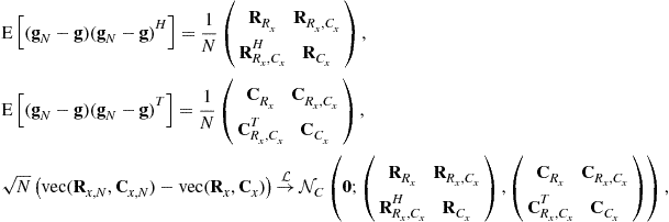
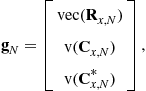
For the second-order statistics
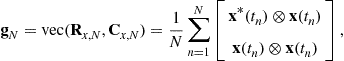
where ![]() and
and ![]() denote, respectively, the vectorization operator that turns a matrix into a vector by stacking the columns of the matrix one below another and the standard Kronecker product of matrices, closed-form expressions of the covariance
denote, respectively, the vectorization operator that turns a matrix into a vector by stacking the columns of the matrix one below another and the standard Kronecker product of matrices, closed-form expressions of the covariance ![]() and complementary covariance
and complementary covariance ![]() matrices (where
matrices (where ![]() for short), and their asymptotic distributions2 have been given [30] for independent measurements, fourth-order arbitrary distributed sources and Gaussian distributed noise:
for short), and their asymptotic distributions2 have been given [30] for independent measurements, fourth-order arbitrary distributed sources and Gaussian distributed noise:
 (16.11)
with
![]() (16.12)
(16.12)

where ![]() for short and
for short and ![]() denotes the vec-permutation matrix which transforms
denotes the vec-permutation matrix which transforms ![]() to
to ![]() for any square matrix
for any square matrix ![]() .
. ![]() ,
, ![]() , and
, and ![]() are defined as for
are defined as for ![]() defined previously and
defined previously and ![]() ,
, ![]() ,
, ![]() . Note that the asymptotic distribution of
. Note that the asymptotic distribution of ![]() has been extended to non independent measurements with arbitrary distributed sources and noise of finite fourth-order moments with
has been extended to non independent measurements with arbitrary distributed sources and noise of finite fourth-order moments with ![]() arbitrarily structured in [20,31].
arbitrarily structured in [20,31].
Consider now the noise orthogonal projector ![]() . Its asymptotic distribution is deduced from the standard first-order perturbation for orthogonal projectors [32] (see also [6]):
. Its asymptotic distribution is deduced from the standard first-order perturbation for orthogonal projectors [32] (see also [6]):
![]() (16.13)
(16.13)
where ![]() ,
, ![]() and
and ![]() is the Moore-Penrose inverse of
is the Moore-Penrose inverse of ![]() . The remainder in (16.13) is a standard
. The remainder in (16.13) is a standard ![]() for a realization of the random matrix
for a realization of the random matrix ![]() , but an
, but an ![]() if
if ![]() is considered as random. The relation (16.13) proves that
is considered as random. The relation (16.13) proves that ![]() is differentiable w.r.t.
is differentiable w.r.t. ![]() in the neighborhood of
in the neighborhood of ![]() and its differential matrix (called also Jacobian matrix) evaluated at
and its differential matrix (called also Jacobian matrix) evaluated at ![]() is
is
![]() (16.14)
(16.14)
Then using the standard theorem of continuity (see, e.g., [33, Theorem B, p. 124]) on regular functions of asymptotically Gaussian statistics, the asymptotic behaviors of ![]() and
and ![]() are directly related:
are directly related:
![]() (16.15)
(16.15)
where ![]() is given for independent measurements, fourth-order arbitrary distributed sources and Gaussian distributed noise, using (16.12) by
is given for independent measurements, fourth-order arbitrary distributed sources and Gaussian distributed noise, using (16.12) by
![]() (16.16)
(16.16)
with ![]() . We see that
. We see that ![]() does not depend on
does not depend on ![]() and the quadrivariances of the sources. Consequently, all subspace-based algorithms are robust to the distribution and to the noncircularity of the sources; i.e., the asymptotic performances are those of the standard complex circular Gaussian case. Note that the asymptotic distribution of
and the quadrivariances of the sources. Consequently, all subspace-based algorithms are robust to the distribution and to the noncircularity of the sources; i.e., the asymptotic performances are those of the standard complex circular Gaussian case. Note that the asymptotic distribution of ![]() and
and ![]() have also been derived under the same assumptions in [27], where it is proved that they do not depend on the quadrivariances of the sources, as well. The asymptotic distributions of
have also been derived under the same assumptions in [27], where it is proved that they do not depend on the quadrivariances of the sources, as well. The asymptotic distributions of ![]() ,
, ![]() and
and ![]() will allow us to derive the statistical performance of arbitrary subspace-based algorithms based on these orthogonal projectors in Section 3.16.4.4.
will allow us to derive the statistical performance of arbitrary subspace-based algorithms based on these orthogonal projectors in Section 3.16.4.4.
Note that the second-order expansion of ![]() w.r.t.
w.r.t. ![]() has been used in [6] to analyze the behavior of the root-MUSIC and root-min-norm algorithms dedicated to ULA, but is useless as far as we are concerned by the asymptotic distribution of the DOAs alone, as it has been specified in [27], where an extension of the root-MUSIC algorithm to noncircular sources has been proposed.
has been used in [6] to analyze the behavior of the root-MUSIC and root-min-norm algorithms dedicated to ULA, but is useless as far as we are concerned by the asymptotic distribution of the DOAs alone, as it has been specified in [27], where an extension of the root-MUSIC algorithm to noncircular sources has been proposed.
Finally, consider now the asymptotic distribution of the signal eigenvalues of ![]() that is useful for the statistical performance analysis of information theoretic criteria (whose MDL criterion popularized by Wax and Kailath [13] is one of the most successful), for the detection of the number
that is useful for the statistical performance analysis of information theoretic criteria (whose MDL criterion popularized by Wax and Kailath [13] is one of the most successful), for the detection of the number ![]() of sources. Let
of sources. Let ![]() denote the eigenvalues of
denote the eigenvalues of ![]() , ordered in decreasing order and
, ordered in decreasing order and ![]() the associated eigenvectors (defined up to a multiplicative unit modulus complex number) of the signal subspace. Then, suppose that for a “small enough” perturbation
the associated eigenvectors (defined up to a multiplicative unit modulus complex number) of the signal subspace. Then, suppose that for a “small enough” perturbation ![]() , the largest
, the largest ![]() associated eigenvalues of the sample covariance
associated eigenvalues of the sample covariance ![]() are
are ![]() . It is proved in [14], extending the work by Kaveh and Barabell [1] to arbitrary distributed independent measurements (16.1) with finite fourth-order moment, not necessarily circular and Gaussian, the following convergence in distribution:
. It is proved in [14], extending the work by Kaveh and Barabell [1] to arbitrary distributed independent measurements (16.1) with finite fourth-order moment, not necessarily circular and Gaussian, the following convergence in distribution:
![]() (16.17)
(16.17)
with ![]() ,
, ![]() , and
, and ![]() for
for ![]() ,
, ![]() is the Kronecker delta,
is the Kronecker delta, ![]() and
and ![]() . In contrast to the circular Gaussian distribution [1], we see that the estimated eigenvalues
. In contrast to the circular Gaussian distribution [1], we see that the estimated eigenvalues ![]() are no longer asymptotically mutually independent. Furthermore, it is proved in [14] that for
are no longer asymptotically mutually independent. Furthermore, it is proved in [14] that for ![]() :
:
 (16.18)
![]() (16.19)
(16.19)
We note that these results are also valid for the augmented covariance matrix ![]() where
where ![]() and
and ![]() are replaced by
are replaced by ![]() and the rank of
and the rank of ![]() , respectively.
, respectively.
3.16.3.1.3 Asymptotic distribution of estimated DOA
In the following, we consider arbitrary DOA algorithms that are in practice “regular” enough.3 More specifically, we assume that the mapping ![]() is
is ![]() -differentiable w.r.t.
-differentiable w.r.t. ![]() in the neighborhood of
in the neighborhood of ![]() , i.e.,
, i.e.,
![]() (16.20)
(16.20)
with ![]() and
and ![]() matrix
matrix ![]() is the
is the ![]() -differential matrix (Jacobian) of the mapping
-differential matrix (Jacobian) of the mapping ![]() evaluated at
evaluated at ![]() . In practice, this matrix is derived from the chain rule by decomposing the algorithm as successive simpler mappings, and in each of these mapping, this matrix is simply deduced from first-order expansions. Then, applying a simple extension of the standard theorem of continuity [33, Theorem B, p. 124] (also called
. In practice, this matrix is derived from the chain rule by decomposing the algorithm as successive simpler mappings, and in each of these mapping, this matrix is simply deduced from first-order expansions. Then, applying a simple extension of the standard theorem of continuity [33, Theorem B, p. 124] (also called ![]() -method), it is straightforwardly proved the following convergence in distribution:
-method), it is straightforwardly proved the following convergence in distribution:
![]() (16.21)
(16.21)
where ![]() and
and ![]() are the covariance and the complementary covariance matrices of the asymptotic distribution of the statistics
are the covariance and the complementary covariance matrices of the asymptotic distribution of the statistics ![]() . We note that for subspace-based algorithms and second-order algorithms based on
. We note that for subspace-based algorithms and second-order algorithms based on ![]() or
or ![]() ,
, ![]() (because the orthogonal projector matrices and the covariance matrices are Hermitian structured), and generally for statistics
(because the orthogonal projector matrices and the covariance matrices are Hermitian structured), and generally for statistics ![]() that contain all conjugate of its components, the mapping
that contain all conjugate of its components, the mapping ![]() is
is ![]() -differentiable w.r.t.
-differentiable w.r.t. ![]() in the neighborhood of
in the neighborhood of ![]() and (16.20) and (16.21) become respectively:
and (16.20) and (16.21) become respectively:
![]() (16.22)
(16.22)
where now, ![]() is the
is the ![]() -differential matrix of the mapping
-differential matrix of the mapping ![]() evaluated at
evaluated at ![]() and
and
![]() (16.23)
(16.23)
3.16.3.1.4 Asymptotic covariance and bias
Under additional regularities of the algorithm ![]() , that are generally satisfied, the covariance of
, that are generally satisfied, the covariance of ![]() is given by
is given by
![]() (16.24)
(16.24)
Using a second-order expansion of ![]() and
and ![]() -calculus, where
-calculus, where ![]() is assumed to be twice-
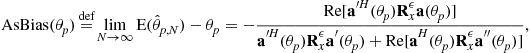
is assumed to be twice-![]() -differentiable, the bias is given by
-differentiable, the bias is given by
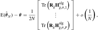 (16.25)
where  is the complex augmented Hessian matrix [34, A2.3] of the
 ![]() th component of the function
th component of the function ![]() at point
at point ![]() and
and  is the augmented covariance of the asymptotic distribution of
 ![]() . In the particular case where
. In the particular case where ![]() is twice-
is twice-![]() -differentiable (see, e.g., the examples given for
-differentiable (see, e.g., the examples given for ![]() -differentiable algorithms (16.22)), i.e.,
-differentiable algorithms (16.22)), i.e.,
 (16.26)
(16.25) reduces to
 (16.27)
We note that relations (16.24), (16.25) and (16.27) are implicitly used in the signal processing literature by simple first and second-order expansions of the estimate ![]() w.r.t. the involved statistics without checking any necessary mathematical conditions concerning the remainder terms of the first and second-order expansions. In fact these conditions are very difficult to prove for the involved mappings
w.r.t. the involved statistics without checking any necessary mathematical conditions concerning the remainder terms of the first and second-order expansions. In fact these conditions are very difficult to prove for the involved mappings ![]() . For example, the following necessary conditions are given in [35, Theorem 4.2.2] for second-order algorithms: (i) the measurements
. For example, the following necessary conditions are given in [35, Theorem 4.2.2] for second-order algorithms: (i) the measurements ![]() are independent with finite eighth moments, (ii) the mapping
are independent with finite eighth moments, (ii) the mapping ![]() is four times
is four times ![]() -differentiable, (iii) the fourth derivative of this mapping and those of its square are bounded. These assumptions that do not depend on the distribution of the measurements are very strong, but fortunately (16.24), (16.25) and (16.27) continue to hold in many cases in which these assumptions are not satisfied, in particular for Gaussian distributed data (see, e.g., [35, Example 4.2.2]).
-differentiable, (iii) the fourth derivative of this mapping and those of its square are bounded. These assumptions that do not depend on the distribution of the measurements are very strong, but fortunately (16.24), (16.25) and (16.27) continue to hold in many cases in which these assumptions are not satisfied, in particular for Gaussian distributed data (see, e.g., [35, Example 4.2.2]).
In practice, (16.24), (16.25), and (16.27) show that the mean square error (MSE)
![]() (16.28)
(16.28)
is then also of order ![]() . Its main contribution comes from the variance term, since the square of the bias is of order
. Its main contribution comes from the variance term, since the square of the bias is of order ![]() . But as empirically observed, this bias contribution may be significant when SNR or
. But as empirically observed, this bias contribution may be significant when SNR or ![]() is not sufficiently large. However, there are very few contributions in the literature, that have derived closed-form bias expressions. Among them, Xu and Cave [36] has considered the bias of the MUSIC algorithm, whose derivation ought to be simplified by using the asymptotic distribution of the orthogonal projector
is not sufficiently large. However, there are very few contributions in the literature, that have derived closed-form bias expressions. Among them, Xu and Cave [36] has considered the bias of the MUSIC algorithm, whose derivation ought to be simplified by using the asymptotic distribution of the orthogonal projector ![]() , rather than those of the sample signal eigenvectors
, rather than those of the sample signal eigenvectors ![]() .
.
3.16.3.2 Cramer-Rao bounds (CRB)
The accuracy measures of performance in terms of covariance and bias of any algorithm, described in the previous section may be of limited interest, unless one has an idea of what the best possible performance is. An important measure of how well a particular DOA finding algorithm performs is the mean square error (MSE) matrix ![]() of the estimation error
of the estimation error ![]() . Among the lower bounds on this matrix, the celebrated Cramer-Rao bound (CRB) is by far the most commonly used. We note that this CRB is indeed deduced from the CRB on the complete unknown parameter
. Among the lower bounds on this matrix, the celebrated Cramer-Rao bound (CRB) is by far the most commonly used. We note that this CRB is indeed deduced from the CRB on the complete unknown parameter ![]() of the parametrized DOA model, for example, given by (16.4) for the circular Gaussian stochastic model. Furthermore, rigorously speaking, this CRB ought to be only used for unbiased estimators and under sufficiently regular distributions of the measurements. Fortunately, these technical conditions are satisfied in practice and due to the property that the bias contribution is often weak w.r.t. the variance term in the mean square error (16.28) for
of the parametrized DOA model, for example, given by (16.4) for the circular Gaussian stochastic model. Furthermore, rigorously speaking, this CRB ought to be only used for unbiased estimators and under sufficiently regular distributions of the measurements. Fortunately, these technical conditions are satisfied in practice and due to the property that the bias contribution is often weak w.r.t. the variance term in the mean square error (16.28) for ![]() , the CRB that lower bounds the covariance matrix of any unbiased estimators is used to lower bound the MSE matrix of any asymptotically unbiased estimator4
, the CRB that lower bounds the covariance matrix of any unbiased estimators is used to lower bound the MSE matrix of any asymptotically unbiased estimator4
![]() (16.29)
(16.29)
with ![]() is given under weak regularity conditions by:
is given under weak regularity conditions by:
![]() (16.30)
(16.30)
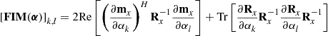
where ![]() is the Fisher information matrix (FIM) given elementwise by
is the Fisher information matrix (FIM) given elementwise by
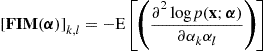 (16.31)
associated with the probability density function ![]() of the measurements
of the measurements ![]() .
.
The main reason for the interest of this CRB is that it is often asymptotically (when the amount ![]() of data is large) tight, i.e., there exist algorithms, such that the stochastic maximum likelihood (ML) estimator (see 3.16.4.2), whose covariance matrices asymptotically achieve this bound. Such estimators are said to be asymptotically efficient. However, at low SNR and/or at low number
of data is large) tight, i.e., there exist algorithms, such that the stochastic maximum likelihood (ML) estimator (see 3.16.4.2), whose covariance matrices asymptotically achieve this bound. Such estimators are said to be asymptotically efficient. However, at low SNR and/or at low number ![]() of snapshots, the CRB is not achieved and is overly optimistic. This is due to the fact that estimators are generally biased in such non-asymptotic cases. For these reasons, other lower bounds are available in the literature, that are more relevant to lower bound the MSE matrices. But unfortunately, their closed-form expressions are much more complex to derive and are generally non interpretable (see, e.g., the Weiss-Weinstein bound in [38]).
of snapshots, the CRB is not achieved and is overly optimistic. This is due to the fact that estimators are generally biased in such non-asymptotic cases. For these reasons, other lower bounds are available in the literature, that are more relevant to lower bound the MSE matrices. But unfortunately, their closed-form expressions are much more complex to derive and are generally non interpretable (see, e.g., the Weiss-Weinstein bound in [38]).
In practice, closed-form expressions of the FIM (16.31) are difficult to obtain for arbitrary distributions of the sources and noise. In general, the involved integrations of (16.31) are solved numerically by replacing the expectations by arithmetical averages over a large number of computer generated measurements. But for Gaussian distributions, there are a plethora of closed-form expressions of ![]() in the literature. And the reason of the popularity of this CRB is the simplicity of the FIM for Gaussian distributions of
in the literature. And the reason of the popularity of this CRB is the simplicity of the FIM for Gaussian distributions of ![]() .
.
3.16.3.2.1 Gaussian stochastic case
On way to derive closed-form expressions of ![]() is to use the extended Slepian-Bangs [39,40] formula, where the FIM (16.31) is given elementwise by
is to use the extended Slepian-Bangs [39,40] formula, where the FIM (16.31) is given elementwise by
 (16.32)
for a circular5 Gaussian ![]() distribution of
distribution of ![]() . But there are generally difficulties to derive compact matrix expressions of the CRB for DOA parameters alone given by
. But there are generally difficulties to derive compact matrix expressions of the CRB for DOA parameters alone given by
![]()
with ![]() where
where ![]() gathers all the nuisance parameters (in many applications, only the DOAs are of interest). Another way, based on the asymptotic efficiency of the ML estimator (under certain regularity conditions) has been used to indirectly derive the CRB on the DOA parameter alone (see 3.16.4.2).
gathers all the nuisance parameters (in many applications, only the DOAs are of interest). Another way, based on the asymptotic efficiency of the ML estimator (under certain regularity conditions) has been used to indirectly derive the CRB on the DOA parameter alone (see 3.16.4.2).
For the circular Gaussian stochastic model of the sources introduced in Section 3.16.2.2, compact matrix expressions of ![]() have been given in the literature, when no a priori information is available on the structure of the spatial covariance
have been given in the literature, when no a priori information is available on the structure of the spatial covariance ![]() of the sources. For example, Stoica et al. [41] have derived the following expression for one parameter per source and uniform white noise (i.e.,
of the sources. For example, Stoica et al. [41] have derived the following expression for one parameter per source and uniform white noise (i.e., ![]() )
)
![]() (16.33)
(16.33)
where ![]() denotes the Hadamard product (i.e., element-wise multiplication),
denotes the Hadamard product (i.e., element-wise multiplication), ![]() is the orthogonal projector on the noise subspace, i.e.,
is the orthogonal projector on the noise subspace, i.e., ![]() and
and ![]() . We note the surprising fact that when the sources are known to be coherent (i.e.,
. We note the surprising fact that when the sources are known to be coherent (i.e., ![]() singular), the associated Gaussian CRB
singular), the associated Gaussian CRB ![]() that includes this prior, keeps the same expression (16.33)[43].
that includes this prior, keeps the same expression (16.33)[43].
As is well known, the importance of this Gaussian CRB formula lies in the fact that circular Gaussian data are rather frequently encountered in applications. Another important point is that under rather general conditions that will be specified in Section 3.16.4.2, the circular complex Gaussian CRB matrix (16.33) is the largest of all CRB matrices among the class of arbitrary complex distributions of the sources with given covariance matrix ![]() (see, e.g., [21, p. 293]). Note that many extensions of (16.33) have been given. For example this formula has been extended to several parameters per source (see, e.g., [44, Appendix D]), to nonuniform white noise (i.e.,
(see, e.g., [21, p. 293]). Note that many extensions of (16.33) have been given. For example this formula has been extended to several parameters per source (see, e.g., [44, Appendix D]), to nonuniform white noise (i.e., ![]() ) and unknown parameterized noise field (i.e.,
) and unknown parameterized noise field (i.e., ![]() ) in [45–47], respectively. Due to the domination of the Gaussian distribution, these bounds have often been denoted in the literature as stochastic CRB (e.g., in [10]) or unconditional CRB (e.g., in [11]), without specifying the involved distribution.
) in [45–47], respectively. Due to the domination of the Gaussian distribution, these bounds have often been denoted in the literature as stochastic CRB (e.g., in [10]) or unconditional CRB (e.g., in [11]), without specifying the involved distribution.
Furthermore, all these closed-form expressions of the CRB have been extended to the noncircular Gaussian stochastic model of the sources in [42,44,48, Appendix D], given associated ![]() expressions satisfying
expressions satisfying
![]()
corresponding to the same covariance matrix ![]() . For example, for a single source, with one parameter
. For example, for a single source, with one parameter ![]() ,
, ![]() decreases monotonically as the second-order noncircularity rate
decreases monotonically as the second-order noncircularity rate ![]() (defined by
(defined by ![]() and satisfying
and satisfying ![]() ) increases from 0 to 1, for which we have, respectively,
) increases from 0 to 1, for which we have, respectively,
 (16.34)
where ![]() is the purely geometrical factor
is the purely geometrical factor ![]() with
with ![]() .
.
If the source covariance ![]() is constrained to have a specific structure, (i.e., if a prior on
is constrained to have a specific structure, (i.e., if a prior on ![]() is taken into account), a specific expression of
is taken into account), a specific expression of ![]() , which integrates this prior ought to be derived, to assess the performance of an algorithm that uses this prior. But unfortunately, the derivation of
, which integrates this prior ought to be derived, to assess the performance of an algorithm that uses this prior. But unfortunately, the derivation of ![]() is very involved and lacks any engineering insight. For example, when it is known that the sources are uncorrelated, the expression given in [49, Theorem 1] of
is very involved and lacks any engineering insight. For example, when it is known that the sources are uncorrelated, the expression given in [49, Theorem 1] of ![]() includes a matrix
includes a matrix ![]() , defined as any matrix, whose columns span the null space of
, defined as any matrix, whose columns span the null space of ![]() . And to the best of our knowledge no closed-form expression of
. And to the best of our knowledge no closed-form expression of ![]() has been published in the important case of coherent sources, when the rank of
has been published in the important case of coherent sources, when the rank of ![]() is fixed strictly smaller than
is fixed strictly smaller than ![]() .
.
Finally, note that the scalar field modeling one component of electromagnetic field or acoustic pressure (16.1) has been extended to vector fields with vector sensors, where associated stochastic CRBs for the DOA (azimuth and elevation) alone have been derived and analyzed for a single source. In particular, the electromagnetic (six electric and magnetic field components) and acoustic (three velocity components and pressure) fields have been considered in [50,51], respectively.
3.16.3.2.2 Gaussian deterministic case
For the deterministic model of the sources introduced in Section 3.16.2.2, the unknown parameter ![]() of
of ![]() is now
is now
![]() (16.35)
(16.35)
Applying the extended Slepian-Bangs formula (16.32) to the circular Gaussian  distribution of
 ![]() , Stoica and Nehorai [11] have obtained the following CRB for the DOA alone:
, Stoica and Nehorai [11] have obtained the following CRB for the DOA alone: ![]() , where
, where ![]() . Furthermore, it was proved in [3] that
. Furthermore, it was proved in [3] that ![]() decreases monotonically with increasing
decreases monotonically with increasing ![]() (and
(and ![]() ). This implies, that if the sources
). This implies, that if the sources ![]() are second-order ergodic sequences,
are second-order ergodic sequences, ![]() has a limit
has a limit ![]() when
when ![]() tends to infinity, and we obtain for large
tends to infinity, and we obtain for large ![]() , the following expression denoted in the literature as deterministic CRB or conditional CRB (e.g., in [11])
, the following expression denoted in the literature as deterministic CRB or conditional CRB (e.g., in [11])
![]() (16.36)
(16.36)
Finally, we remark that the CRB for near-field DOA localization has been much less studied than the far-field one. To the best of our knowledge, only papers [52–54] have given and analyzed closed-form expressions of the stochastic and deterministic CRB, and furthermore in the particular case of a single source for specific arrays. For a ULA where the DOA parameters are the azimuth ![]() and the range
and the range ![]() , based on the DOA algorithms, the steering vector (16.2) has been approximated in [53] by
, based on the DOA algorithms, the steering vector (16.2) has been approximated in [53] by
![]()
where ![]() and
and ![]() are the so-called electric angles connected to the physical parameters
are the so-called electric angles connected to the physical parameters ![]() and
and ![]() by
by ![]() and
and ![]() . Then in [52], the exact propagation model
. Then in [52], the exact propagation model
![]()
has been used, that has revealed interesting features and interpretations not shown in [53]. Very recently, the uniform circular array (UCA) has been investigated in [54] in which the exact propagation model is now:

where ![]() and
and ![]() denote the radius of the UCA, the azimuth and the elevation of the source. Note that in contrast to the closed-form expressions given in [53] and [52], the ones given in [54] relate the near and far-field CRB on the azimuth and elevation by very simple expressions.
denote the radius of the UCA, the azimuth and the elevation of the source. Note that in contrast to the closed-form expressions given in [53] and [52], the ones given in [54] relate the near and far-field CRB on the azimuth and elevation by very simple expressions.
3.16.3.2.3 Non Gaussian case
The stochastic CRB for the DOA appears to be prohibitive to compute for non-Gaussian sources. To cope with this difficulty, the deterministic model for the sources has been proposed for its simplicity. But in contrast to the stochastic ML estimator, the corresponding deterministic (or conditional) ML method does not asymptotically achieve this deterministic CRB, because the deterministic likelihood function does not meet the required regularity conditions (see Section 3.16.4.2). Consequently, this deterministic CRB is only a nonattainable lower bound on the covariance of any unbiased DOA estimator for arbitrary non-Gaussian distributions of the sources. So, it is useful to have explicit expressions of the stochastic CRB under non-Gaussian distributions.
To the best of our knowledge, such stochastic CRBs have only been given in the case of binary phase-shift keying (BPSK), quaternary phase-shift keying (QPSK) signal waveforms [55] and then, to arbitrary ![]() -ary square QAM constellation [56], and for a single source only. In these works, it is assumed Nyquist shaping and ideal sample timing apply so that the intersymbol interference at each symbol spaced sampling instance can be ignored. In the absence of frequency offset but with possible phase offset, the signals at the output of the matched filter can be represented as
-ary square QAM constellation [56], and for a single source only. In these works, it is assumed Nyquist shaping and ideal sample timing apply so that the intersymbol interference at each symbol spaced sampling instance can be ignored. In the absence of frequency offset but with possible phase offset, the signals at the output of the matched filter can be represented as ![]() , where
, where ![]() are independent identically distributed random symbols taking values
are independent identically distributed random symbols taking values ![]() for BPSK symbols and
for BPSK symbols and ![]() with
with ![]() for
for ![]() -ary square QAM symbols, where
-ary square QAM symbols, where ![]() is the intersymbol distance in the I/Q plane, which is adjusted such that
is the intersymbol distance in the I/Q plane, which is adjusted such that ![]() . For these discrete sources, the unknown parameter of this stochastic model is
. For these discrete sources, the unknown parameter of this stochastic model is
![]()
and it has been proved in [55,56] that the parameters ![]() and
and ![]() are decoupled in the associated FIM. This allows one to derive closed-form expressions of the so called non-data-aided (NDA) CRBs on the parameter
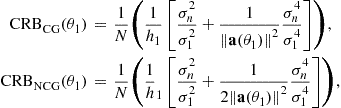
are decoupled in the associated FIM. This allows one to derive closed-form expressions of the so called non-data-aided (NDA) CRBs on the parameter ![]() alone. In particular, it has been proved [55] that for a BPSK and QPSK source, that is respectively rectilinear and second-order circular, we have
alone. In particular, it has been proved [55] that for a BPSK and QPSK source, that is respectively rectilinear and second-order circular, we have
 (16.37)
where ![]() and
and ![]() are given by (16.34) and with
are given by (16.34) and with ![]() and
and ![]() is the following decreasing function of
is the following decreasing function of ![]() :
: ![]() . Equation (16.37) is illustrated in Figure 16.1 for a ULA of
. Equation (16.37) is illustrated in Figure 16.1 for a ULA of ![]() sensors spaced a half-wavelength apart. We see from this figure that the CRBs under the non-circular [resp. circular] complex Gaussian distribution are tight upper bounds on the CRBs under the BPSK [resp. QPSK] distribution at very low and very high SNRs only. Finally, note that among the numerous results of [55,56], these stochastic NDA CRBs have been compared with those obtained with different a priori knowledge. In particular, it has been proved that in the presence of any unknown phase offset (i.e., non-coherent estimation), the ultimate achievable performance on the NDA DOA estimates holds almost the same irrespectively of the modulation order
sensors spaced a half-wavelength apart. We see from this figure that the CRBs under the non-circular [resp. circular] complex Gaussian distribution are tight upper bounds on the CRBs under the BPSK [resp. QPSK] distribution at very low and very high SNRs only. Finally, note that among the numerous results of [55,56], these stochastic NDA CRBs have been compared with those obtained with different a priori knowledge. In particular, it has been proved that in the presence of any unknown phase offset (i.e., non-coherent estimation), the ultimate achievable performance on the NDA DOA estimates holds almost the same irrespectively of the modulation order ![]() . However, the NDA CRBs obtained in the absence of phase offset (i.e., coherent estimation) vary, in the high SNR region, from one modulation order to another.
. However, the NDA CRBs obtained in the absence of phase offset (i.e., coherent estimation) vary, in the high SNR region, from one modulation order to another.

Finally note that the ML estimation of the DOAs of these discrete sources has been proposed [57], where the maximization of the ML criterion (which is rather involved) is iteratively carried out by the expectation maximization (EM) algorithm. Adapted to the distribution of these sources, this approach allows one to account for any arbitrary noise covariance ![]() as soon as
as soon as ![]() is Gaussian distributed.
is Gaussian distributed.
3.16.3.3 Asymptotically minimum variance bounds (AMVB)
To assess the performance of an algorithm based on a specific statistic ![]() built on
built on ![]() , it is interesting to compare the asymptotic covariance
, it is interesting to compare the asymptotic covariance ![]() (16.21) or (16.23) to an attainable lower bound that depends on the statistic
(16.21) or (16.23) to an attainable lower bound that depends on the statistic ![]() only. The asymptotically minimum variance bound (AMVB) is such a bound. Furthermore, we note that the CRB appears to be prohibitive to compute for non-Gaussian sources and noise, except in simple cases and consequently this AMVB can be used as an useful benchmark against which potential estimates
only. The asymptotically minimum variance bound (AMVB) is such a bound. Furthermore, we note that the CRB appears to be prohibitive to compute for non-Gaussian sources and noise, except in simple cases and consequently this AMVB can be used as an useful benchmark against which potential estimates ![]() are tested. To extend the derivations of Porat and Friedlander [58] concerning this AMVB to complex-valued measurements, two additional conditions to those introduced in Section 3.16.3.1.1 must be satisfied:
are tested. To extend the derivations of Porat and Friedlander [58] concerning this AMVB to complex-valued measurements, two additional conditions to those introduced in Section 3.16.3.1.1 must be satisfied:
iii. The involved function ![]() that defines the considered algorithm must be
that defines the considered algorithm must be ![]() -differentiable, i.e., must satisfy (16.22). In practice, it is sufficient to add conjugate components to all complex-valued components of
-differentiable, i.e., must satisfy (16.22). In practice, it is sufficient to add conjugate components to all complex-valued components of ![]() , as in example (16.41);
, as in example (16.41);
iv. The covariance ![]() of the asymptotic distribution of
of the asymptotic distribution of ![]() must be nonsingular. To satisfy this latter condition, the components of
must be nonsingular. To satisfy this latter condition, the components of ![]() that are random variables, must be asymptotically linearly independent. Consequently the redundancies in
that are random variables, must be asymptotically linearly independent. Consequently the redundancies in ![]() must be withdrawn.
must be withdrawn.
Under these four conditions, the covariance matrix ![]() of the asymptotic distribution of any estimator
of the asymptotic distribution of any estimator ![]() built on the statistics
built on the statistics ![]() is bounded below by
is bounded below by ![]() :
:
![]() (16.38)
(16.38)
where ![]() is the
is the ![]() matrix
matrix ![]() .
.
Furthermore, this lowest bound ![]() is asymptotically tight, i.e., there exists an algorithm
is asymptotically tight, i.e., there exists an algorithm ![]() whose covariance of its asymptotic distribution satisfies (16.38) with equality. The following nonlinear least square algorithm is an AMV second-order algorithm:
whose covariance of its asymptotic distribution satisfies (16.38) with equality. The following nonlinear least square algorithm is an AMV second-order algorithm:
![]() (16.39)
(16.39)
where we have emphasized here the dependence of ![]() on the unknown DOA
on the unknown DOA ![]() . In practice, it is difficult to optimize the nonlinear function (16.39), where it involves the computation of
. In practice, it is difficult to optimize the nonlinear function (16.39), where it involves the computation of ![]() . Porat and Friedlander proved for the real case in [59] that the lowest bound (16.38) is also obtained if an arbitrary weakly consistent estimate
. Porat and Friedlander proved for the real case in [59] that the lowest bound (16.38) is also obtained if an arbitrary weakly consistent estimate ![]() of
of ![]() is used in (16.39), giving the simplest algorithm:
is used in (16.39), giving the simplest algorithm:
![]() (16.40)
(16.40)
This property has been extended to the complex case in [60].
This AMVB and AMV algorithm have been applied to second-order algorithms that exploit both ![]() and
and ![]() in [24]. In this case, to fulfill the previously mentioned conditions (i)–(iv), the second-order statistics
in [24]. In this case, to fulfill the previously mentioned conditions (i)–(iv), the second-order statistics ![]() are given by
are given by
 (16.41)
where ![]() denotes the operator obtained from
denotes the operator obtained from ![]() by eliminating all supradiagonal elements of a matrix. Finally, note that these AMVB and AMV DOA finding algorithm have been also derived for fourth-order statistics by splitting the measurements and statistics
by eliminating all supradiagonal elements of a matrix. Finally, note that these AMVB and AMV DOA finding algorithm have been also derived for fourth-order statistics by splitting the measurements and statistics ![]() into its real and imaginary parts in [60].
into its real and imaginary parts in [60].
3.16.3.4 Relations between AMVB and CRB: projector statistics
The AMVB based on any statistics is generally lower bounded by the CRB because this later bound concerns arbitrary functions of the measurements ![]() . But it has been proved in [44], that the AMVB associated with the different estimated projectors
. But it has been proved in [44], that the AMVB associated with the different estimated projectors ![]() ,
, ![]() and
and ![]() introduced in Section 3.16.3.1.2, which are functions of the second-order statistics of the measurements, attains the stochastic CRB in the case of circular or noncircular Gaussian signals. Consequently, there always exist asymptotically efficient subspace-based DOA algorithms in the Gaussian context.
introduced in Section 3.16.3.1.2, which are functions of the second-order statistics of the measurements, attains the stochastic CRB in the case of circular or noncircular Gaussian signals. Consequently, there always exist asymptotically efficient subspace-based DOA algorithms in the Gaussian context.
To prove this asymptotic efficiency, i.e.,
![]() (16.42)
(16.42)
and
![]() (16.43)
(16.43)
the condition (iv) of Section 3.16.3.3 that is not satisfied [61] for these statistics ought to be extended and consequently the results (16.38) and (16.39) must be modified as well, because here ![]() is singular.
is singular.
In this singular case, it has been proved [61] that if the condition (iv) in the necessary conditions (i)–(iv) is replaced by the new condition ![]() , (16.38) and (16.39) becomes respectively
, (16.38) and (16.39) becomes respectively
![]() (16.44)
(16.44)
and
![]() (16.45)
(16.45)
And it is proved that the three statistics ![]() ,
, ![]() , and
, and ![]() satisfy the conditions (i)–(iii) and (v) and thus satisfy results (16.44) and (16.45).
satisfy the conditions (i)–(iii) and (v) and thus satisfy results (16.44) and (16.45).
Finally, note that this efficiency property of the orthogonal projectors extends to the model of spatially correlated noise, for which ![]() where
where ![]() is a known positive definite matrix. In this case, for example, the orthogonal projector
is a known positive definite matrix. In this case, for example, the orthogonal projector ![]() defined after whitening
defined after whitening

satisfies
![]()
where ![]() is insensitive to the choice of the square root
is insensitive to the choice of the square root ![]() of
of ![]() , and is no longer a projection matrix.
, and is no longer a projection matrix.
3.16.4 Asymptotic distribution of estimated DOA
We are now specifying in this section the asymptotic statistical performances of the main DOA algorithms that may be classified into three main categories, namely beamforming-based, maximum like-lihood and moments-based algorithms.
3.16.4.1 Beamforming-based algorithms
Among the so-called beamforming-based algorithms, also referred to as low-resolution, compared to the parametric algorithms, the conventional (Bartlett) beamforming and Capon beamforming are the most referenced representatives of this family. These algorithms do not make any assumption on the covariance structure of the data, but the functional form of the steering vector ![]() is assumed perfectly known. These estimators
is assumed perfectly known. These estimators ![]() are given by the
are given by the ![]() highest (supposed isolated) maximizer and minimizer in
highest (supposed isolated) maximizer and minimizer in ![]() of the respective following criteria:
of the respective following criteria:
![]() (16.46)
(16.46)
where ![]() is the unbiased sample estimate
is the unbiased sample estimate ![]() and
and ![]() is either the biased estimate
is either the biased estimate ![]() or the unbiased estimate
or the unbiased estimate ![]() (that both give the same estimate
(that both give the same estimate ![]() ). Note that these algorithms extend to
). Note that these algorithms extend to ![]() parameters per source, where
parameters per source, where ![]() is replaced by
is replaced by ![]() in (16.46).
in (16.46).
For arbitrary noise field (i.e., arbitrary noise covariance ![]() ) and/or an arbitrary number
) and/or an arbitrary number ![]() of sources, the estimate
of sources, the estimate ![]() given by these two algorithms are non-consistent, i.e.,
given by these two algorithms are non-consistent, i.e.,
![]()
and asymptotically biased. The asymptotic bias ![]() can be straightforwardly derived by a second-order expansion of the criterion
can be straightforwardly derived by a second-order expansion of the criterion ![]() around each true values
around each true values ![]() (with
(with ![]() [resp.,
[resp., ![]() ] for the conventional [resp. Capon] algorithm), but noting that
] for the conventional [resp. Capon] algorithm), but noting that ![]() is a maximizer or minimizer
is a maximizer or minimizer ![]() of
of ![]() or
or ![]() , respectively. The following value is obtained [62]
, respectively. The following value is obtained [62]
 (16.47)
with ![]() and
and ![]() .
.
Following the methodology of Section 3.16.3.1.2, the additional bias for finite value of ![]() , that is of order
, that is of order ![]() can be derived, which gives
can be derived, which gives
![]()
see, e.g., the involved expression of ![]() for the Capon algorithm [62, rel. (35)].
for the Capon algorithm [62, rel. (35)].
In the same way, the covariance ![]() which is of order
which is of order ![]() can be derived. It is obtained with
can be derived. It is obtained with ![]()
![]()
see, e.g., the involved expression [50, rel. (24)] of ![]() associated with a source for several parameters per source. The relative values of the asymptotic bias, additional bias and standard deviation depend on the SNR,
associated with a source for several parameters per source. The relative values of the asymptotic bias, additional bias and standard deviation depend on the SNR, ![]() and
and ![]() , but in practice the standard deviation is typically dominant over the asymptotic bias and additional bias (see examples given in [62]).
, but in practice the standard deviation is typically dominant over the asymptotic bias and additional bias (see examples given in [62]).
Finally, note that in the particular case of a single source, uniform white noise (![]() ) and an arbitrary number
) and an arbitrary number ![]() of parameters of the source (here
of parameters of the source (here ![]() ), it has been proved [63], that
), it has been proved [63], that ![]() given by these two beamforming-based algorithms is asymptotically unbiased (
given by these two beamforming-based algorithms is asymptotically unbiased (![]() given by (16.47) is zero), if and only if
given by (16.47) is zero), if and only if ![]() is constant. Furthermore, based on the general expressions (16.48) of the FIM6
is constant. Furthermore, based on the general expressions (16.48) of the FIM6
![]() (16.48)
(16.48)
where ![]() is defined here by
is defined here by ![]() , for
, for ![]() parameters associated with a single source, and expression [50, rel. (24)] of
parameters associated with a single source, and expression [50, rel. (24)] of ![]() specialized to
specialized to ![]() , it has been proved that
, it has been proved that ![]() , i.e., the conventional and Capon algorithms are asymptotically efficient, if and only if
, i.e., the conventional and Capon algorithms are asymptotically efficient, if and only if ![]() is constant.
is constant.
3.16.4.2 Maximum likelihood algorithms
3.16.4.2.1 Stochastic and deterministic ML algorithms
As discussed in Section 3.16.2.2, the two main models for the sensor array problem in Gaussian noise, corresponding to stochastic and deterministic modeling of the source signals lead to two different Gaussian distributions of the measurements ![]() , and consequently to two different log-likelihoods
, and consequently to two different log-likelihoods ![]() , where the unknown parameter
, where the unknown parameter ![]() is respectively given by (16.4) and (16.35).
is respectively given by (16.4) and (16.35).
With some algebraic effort, the stochastic ML criterion ![]() can be concentrated w.r.t.
can be concentrated w.r.t. ![]() and
and ![]() (see, e.g., [64,65]), thus reducing the dimension of the required numerical maximization to the required
(see, e.g., [64,65]), thus reducing the dimension of the required numerical maximization to the required ![]() DOAs
DOAs ![]() and giving the following optimization problem:
and giving the following optimization problem:
![]() (16.49)
(16.49)
with
![]() (16.50)
(16.50)
where
![]() (16.51)
(16.51)
where ![]() is the orthogonal projector onto the null space of
is the orthogonal projector onto the null space of ![]() . Despite its reduction of the parameter space,
. Despite its reduction of the parameter space, ![]() is a complicated nonlinear expression in
is a complicated nonlinear expression in ![]() , that cannot been analytically minimized. Consequently, numerical optimization procedures are required.
, that cannot been analytically minimized. Consequently, numerical optimization procedures are required.
Remark that in this modeling, the obvious a priori information that ![]() is positive semi-definite has not been taken into account. This knowledge, and more generally, the prior that
is positive semi-definite has not been taken into account. This knowledge, and more generally, the prior that ![]() is positive semi-definite of rank
is positive semi-definite of rank ![]() smaller or equal than
smaller or equal than ![]() can be included in the modeling by the parametrization
can be included in the modeling by the parametrization ![]() , where
, where ![]() is a
is a ![]() lower triangular matrix. But this modification will have no effect for “large enough
lower triangular matrix. But this modification will have no effect for “large enough ![]() ” since
” since ![]() given by (16.51) is a weakly consistent estimate of
given by (16.51) is a weakly consistent estimate of ![]() [12]. And since this new parametrization leads to significantly more involved optimization, the unrestricted parametrization of
[12]. And since this new parametrization leads to significantly more involved optimization, the unrestricted parametrization of ![]() used in (16.50) appears to be preferable.
used in (16.50) appears to be preferable.
Due to the quadratic dependence of the deterministic ML criterion ![]() in the parameters
in the parameters ![]() , its concentration w.r.t.
, its concentration w.r.t. ![]() and
and ![]() is much more simpler than for the stochastic ML criterion. It gives the following new ML estimator:
is much more simpler than for the stochastic ML criterion. It gives the following new ML estimator:
![]() (16.52)
(16.52)
with
![]() (16.53)
(16.53)
Comparing (16.53) and (16.50), we see that the dependence in ![]() of the DML criterion is simpler than for the SML criterion. But both criteria require nonlinear
of the DML criterion is simpler than for the SML criterion. But both criteria require nonlinear ![]() th-dimensional minimizations with a large number of local minima that give two different estimates
th-dimensional minimizations with a large number of local minima that give two different estimates ![]() , except for a single source for which the minimization of (16.53) and (16.50) reduce to the maximization of the common criteria
, except for a single source for which the minimization of (16.53) and (16.50) reduce to the maximization of the common criteria
![]()
This implies that when the norm of the steering vector ![]() is constant (which is generally assumed), the conventional and Capon beamforming, SML and DML algorithms coincide and thus conventional and Capon beamforming and DML algorithms inherit the asymptotical efficiency of the SML algorithm. Note that this property extends to several parameters per source.
is constant (which is generally assumed), the conventional and Capon beamforming, SML and DML algorithms coincide and thus conventional and Capon beamforming and DML algorithms inherit the asymptotical efficiency of the SML algorithm. Note that this property extends to several parameters per source.
3.16.4.2.2 Asymptotic properties of ML algorithms
We consider in this Subsection, the asymptotic properties of DML or SML algorithms used under the respectively, deterministic and circular Gaussian stochastic modeling of the sources. In the field of asymptotic performance characterization of DML or SML algorithms, asymptotic generally refers to either the number ![]() of snapshots or the SNR value.
of snapshots or the SNR value.
First, consider the asymptotic properties w.r.t. ![]() , that are the most known. Under regularity conditions that are satisfied by the SML algorithm, the general properties of ML estimation states that
, that are the most known. Under regularity conditions that are satisfied by the SML algorithm, the general properties of ML estimation states that ![]() is consistent and asymptotically efficient and Gaussian distributed, more precisely
is consistent and asymptotically efficient and Gaussian distributed, more precisely
![]() (16.54)
(16.54)
where ![]() is given by (16.33). This property of the SML algorithm extends to nonuniform white and unknown parameterized noise field in [45,46], respectively, and to general noncircular Gaussian stochastic modeling of the sources with the associated
is given by (16.33). This property of the SML algorithm extends to nonuniform white and unknown parameterized noise field in [45,46], respectively, and to general noncircular Gaussian stochastic modeling of the sources with the associated ![]() [42,48]. Note that to circumvent the difficulty to extract the “
[42,48]. Note that to circumvent the difficulty to extract the “![]() corner” from the inverse of
corner” from the inverse of ![]() , a matrix closed-form expression of
, a matrix closed-form expression of ![]() has been first obtained in an indirect manner by an asymptotic analysis of the SML estimator [10,11]. Then, only 10 years later, this CRB has been obtained directly from the extended Slepian-Bangs formula [41,45].
has been first obtained in an indirect manner by an asymptotic analysis of the SML estimator [10,11]. Then, only 10 years later, this CRB has been obtained directly from the extended Slepian-Bangs formula [41,45].
As for the DML algorithm, since the signal waveforms themselves are regarded as unknown parameters, it follows that the number of unknown parameters ![]() (16.35) in the modeling, grows without limit with increasing
(16.35) in the modeling, grows without limit with increasing ![]() , the general asymptotic properties of the ML no longer apply. More precisely, the DML estimate of
, the general asymptotic properties of the ML no longer apply. More precisely, the DML estimate of ![]() is weakly consistent, whereas the DML estimate of
is weakly consistent, whereas the DML estimate of ![]() is inconsistent. The asymptotic distribution of
is inconsistent. The asymptotic distribution of ![]() has been derived in [4,66]
has been derived in [4,66]
![]() (16.55)
(16.55)
with
![]() (16.56)
(16.56)
where ![]() is given by (16.36). Note that the inequality
is given by (16.36). Note that the inequality ![]() in (16.56) does not follow from the Cramer-Rao inequality theory directly, because the Cramer-Rao inequality requires that the number of unknown parameters be finite. As the number of real-valued parameters in
in (16.56) does not follow from the Cramer-Rao inequality theory directly, because the Cramer-Rao inequality requires that the number of unknown parameters be finite. As the number of real-valued parameters in ![]() (16.35) is
(16.35) is ![]() , it increases with
, it increases with ![]() and the Cramer-Rao inequality does not apply here. Note that the DML estimates of
and the Cramer-Rao inequality does not apply here. Note that the DML estimates of ![]() are indeed asymptotically unbiased, despite being non-consistent.
are indeed asymptotically unbiased, despite being non-consistent.
Furthermore, it has been proved in [4], that if the DML algorithm is used under the circular Gaussian stochastic modeling of the sources, the asymptotic distribution (16.54) of ![]() is preserved. But under this assumption on the sources, the DML algorithm is suboptimal, and thus
is preserved. But under this assumption on the sources, the DML algorithm is suboptimal, and thus ![]() . Finally comparing directly the expressions (16.33) and (16.36) of the Cramer-Rao bound by applying the matrix inversion lemma, it is straightforward to prove that
. Finally comparing directly the expressions (16.33) and (16.36) of the Cramer-Rao bound by applying the matrix inversion lemma, it is straightforward to prove that ![]() . This allows one to relate
. This allows one to relate ![]() ,
, ![]() ,
, ![]() , and
, and ![]() by the following relation:
by the following relation:
![]() (16.57)
(16.57)
In particular, for a single source with ![]() parameters, we have
parameters, we have
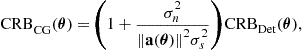 (16.58)
with ![]() , where
, where ![]() is given by (16.48).
is given by (16.48).
Finally, note an asymptotic robustness property [10,11] of the SML and DML algorithms that states that the asymptotic distribution of ![]() and
and ![]() is preserved whatever the modeling of the source: circular Gaussian distributed with
is preserved whatever the modeling of the source: circular Gaussian distributed with ![]() or modeled by arbitrary second-order ergodic signals with
or modeled by arbitrary second-order ergodic signals with ![]() . We will present a more general asymptotic robustness property that applies to a large category of second-order algorithms in Section 3.16.4.3. The fact that the SML algorithm always outperforms (for
. We will present a more general asymptotic robustness property that applies to a large category of second-order algorithms in Section 3.16.4.3. The fact that the SML algorithm always outperforms (for ![]() ) the DML algorithm, provides strong justifications for the appropriateness of the stochastic modeling of sources for the DOA estimation problem.
) the DML algorithm, provides strong justifications for the appropriateness of the stochastic modeling of sources for the DOA estimation problem.
Consider now, the asymptotic properties of the SML and DML algorithms w.r.t. SNR, used under their respective source model assumptions. It has been proved in [28], that under the circular Gaussian assumption of the sources, the SML estimates ![]() is asymptotically (w.r.t. SNR) non-Gaussian distributed and non-efficient, i.e.,
is asymptotically (w.r.t. SNR) non-Gaussian distributed and non-efficient, i.e., ![]() converges in distribution to a non-Gaussian distribution, when
converges in distribution to a non-Gaussian distribution, when ![]() tends to zero, with
tends to zero, with ![]() fixed, with
fixed, with ![]() . In practice,
. In practice, ![]() is non-Gaussian distributed and non-efficient at high SNR, only for a very small number
is non-Gaussian distributed and non-efficient at high SNR, only for a very small number ![]() of snapshots.7 For example, for a single source, using (16.37), it is proved in [28] that
of snapshots.7 For example, for a single source, using (16.37), it is proved in [28] that
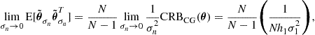
(see (16.34) for the second equality), where ![]() is defined just after (16.34). These properties contrast with the DML algorithm used under the deterministic modeling of the sources, which is proved [67] to be asymptotically (w.r.t. SNR) Gaussian distributed and efficient, i.e.,
is defined just after (16.34). These properties contrast with the DML algorithm used under the deterministic modeling of the sources, which is proved [67] to be asymptotically (w.r.t. SNR) Gaussian distributed and efficient, i.e., ![]()
![]() when
when ![]() tends to zero, with
tends to zero, with ![]() arbitrary fixed. These results are consistent with those of [11]. In practice for very high SNR and “not too small”
arbitrary fixed. These results are consistent with those of [11]. In practice for very high SNR and “not too small” ![]() , (16.57) becomes
, (16.57) becomes
![]() (16.59)
(16.59)
Furthermore, it has been proved in [11], that (16.59) is also valid for ![]() . The asymptotic distribution of the DOA estimate w.r.t.
. The asymptotic distribution of the DOA estimate w.r.t. ![]() (for finite data) of the SML and DML algorithms has been studied in [68]. The strong consistency has been proved for both ML algorithms. Furthermore, unlike the previously studied large sample case, the asymptotic covariance matrices of the DOA estimates coincide with the deterministic CRB (16.36) for the SML and DML algorithms. The asymptotic distribution of the DOA estimates given by subspace-based algorithms has been studied in [29], when
(for finite data) of the SML and DML algorithms has been studied in [68]. The strong consistency has been proved for both ML algorithms. Furthermore, unlike the previously studied large sample case, the asymptotic covariance matrices of the DOA estimates coincide with the deterministic CRB (16.36) for the SML and DML algorithms. The asymptotic distribution of the DOA estimates given by subspace-based algorithms has been studied in [29], when ![]() ,
, ![]() , whereas
, whereas ![]() converges to a strictly positive constant. In this asymptotic regime, it is proved, in particular, that these traditional DOA estimates are not consistent. The threshold and the so-called subspace swap of the SML and MUSIC algorithms have been studied w.r.t.
converges to a strictly positive constant. In this asymptotic regime, it is proved, in particular, that these traditional DOA estimates are not consistent. The threshold and the so-called subspace swap of the SML and MUSIC algorithms have been studied w.r.t. ![]() ,
, ![]() and SNR (see, e.g., [69]). Furthermore, a new consistent subspace-based estimate has been proposed, which outperforms the standard subspace-based methods for values of
and SNR (see, e.g., [69]). Furthermore, a new consistent subspace-based estimate has been proposed, which outperforms the standard subspace-based methods for values of ![]() and
and ![]() of the same order of magnitude [29].
of the same order of magnitude [29].
3.16.4.2.3 Large sample ML approximations
Since the SML and DML algorithms are often deemed exceedingly complex, suboptimal algorithms are of interest. Many such algorithms have been proposed in the literature and surprisingly, some of them are asymptotically as accurate as the ML algorithms, but with a reduced computational cost. These algorithms have been derived, either by approximations of the ML criteria by neglecting terms that do not affect the asymptotic properties of the estimates, or by using a purely geometrical point of view. We present this latter approach that allows one to unify a large number of algorithms [12]. These algorithms rely on the geometrical properties of the spectral decomposition of the covariance matrix ![]() :
:
![]()
with ![]() ,
, ![]() , and
, and ![]() where
where ![]() is the rank of
is the rank of ![]() , associated with the consistent estimates
, associated with the consistent estimates
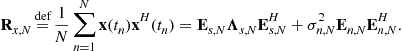 (16.60)
These algorithms can be classified as signal subspace-based and noise subspace-based fitting algorithms. The former algorithms based on ![]() are given by the following optimization:
are given by the following optimization:
![]() (16.61)
(16.61)
where ![]() is a weighting
is a weighting ![]() positive definite matrix to be specified. And the latter algorithms based on
positive definite matrix to be specified. And the latter algorithms based on ![]() , that is valid only if the source covariance matrix is nonsingular (
, that is valid only if the source covariance matrix is nonsingular (![]() ), are given by
), are given by
![]() (16.62)
(16.62)
where ![]() is a weighting
is a weighting ![]() positive definite matrix to be specified.
positive definite matrix to be specified.
Introduced from a purely geometrical point of view, these two classes of algorithms present unexpected relations with the previously described ML algorithms. First, for arbitrary positive definite weighting matrices ![]() and
and ![]() , the estimates
, the estimates ![]() and
and ![]() given respectively by (16.61) and (16.62), are weakly consistent. Second, for the weighting matrices that give the lowest covariance matrix of the asymptotic distribution of
given respectively by (16.61) and (16.62), are weakly consistent. Second, for the weighting matrices that give the lowest covariance matrix of the asymptotic distribution of ![]() and
and ![]() , that are respectively given [12] by
, that are respectively given [12] by
![]()
where ![]() denotes here the true value of the DOAs, the associated estimates
denotes here the true value of the DOAs, the associated estimates ![]() and
and ![]() are asymptotically equivalent to
are asymptotically equivalent to ![]() (i.e.,
(i.e., ![]() and
and ![]() in probability as
in probability as ![]() ) and thus have the same asymptotic distribution that the SML algorithm. Furthermore and fortunately, this property extends for any weakly consistent estimates
) and thus have the same asymptotic distribution that the SML algorithm. Furthermore and fortunately, this property extends for any weakly consistent estimates ![]() and
and ![]() of respectively
of respectively ![]() and
and ![]() , e.g., derived from the spectral decomposition of the sample covariance matrix
, e.g., derived from the spectral decomposition of the sample covariance matrix ![]() (16.60) with
(16.60) with ![]() is the average of
is the average of ![]() smallest eigenvalues of
smallest eigenvalues of ![]() and with
and with ![]() is replaced by a weakly consistent estimates of
is replaced by a weakly consistent estimates of ![]() . This implies a two steps procedure to run the optimal noise subspace-based fitting algorithm. Due to this drawback, the signal subspace-based fitting algorithm with the weighting
. This implies a two steps procedure to run the optimal noise subspace-based fitting algorithm. Due to this drawback, the signal subspace-based fitting algorithm with the weighting ![]() , denoted weighted subspace fitting (WSF) algorithm, is preferred to the noise subspace-based fitting algorithms.
, denoted weighted subspace fitting (WSF) algorithm, is preferred to the noise subspace-based fitting algorithms.
Finally, note that this algorithm is based on eigenvalues and eigenvectors of the sample covariance matrix ![]() . This contrasts with the subspace-based algorithms whose asymptotic statistical properties will be studied in Section 3.16.4.4 that are based on the noise or signal orthogonal projector
. This contrasts with the subspace-based algorithms whose asymptotic statistical properties will be studied in Section 3.16.4.4 that are based on the noise or signal orthogonal projector ![]() associated with
associated with ![]() only. Note that general properties of subspace-based estimators focused on asymptotic invariance of these estimators have been given in [70].
only. Note that general properties of subspace-based estimators focused on asymptotic invariance of these estimators have been given in [70].
3.16.4.3 Second-order algorithms
Most of the narrowband DOA algorithms presented in the literature are second-order algorithms, i.e., are based on the sample covariance ![]() or more generally on
or more generally on ![]()
![]() . To prove common properties of this class of algorithm, it is useful to use the functional analysis presented in Section 3.16.3.1.1
. To prove common properties of this class of algorithm, it is useful to use the functional analysis presented in Section 3.16.3.1.1
![]() (16.63)
(16.63)
in which any second-order algorithm is a mapping alg that generally satisfies
![]() (16.64)
(16.64)
but not necessarily for all ![]() Hermitian positive semi-definite matrix
Hermitian positive semi-definite matrix ![]() . Depending on the a priori knowledge about
. Depending on the a priori knowledge about ![]() , that is required by the second-order algorithms alg, different constraints are satisfied by the
, that is required by the second-order algorithms alg, different constraints are satisfied by the ![]() -differential matrix
-differential matrix ![]() of the algorithm at the point
of the algorithm at the point ![]() (16.22). In particular, it has been proved the following main two constraints [20]:
(16.22). In particular, it has been proved the following main two constraints [20]:
![]() (16.65)
(16.65)
![]() (16.66)
(16.66)
Using these constraints, the general expression ![]() of the covariance of the asymptotic distribution of the sample covariance
of the covariance of the asymptotic distribution of the sample covariance ![]() [31] obtained under mild conditions for non independent measurements with arbitrary distributed sources and noise of finite fourth-order moments, and the general relation (16.23), that links
[31] obtained under mild conditions for non independent measurements with arbitrary distributed sources and noise of finite fourth-order moments, and the general relation (16.23), that links ![]() and
and ![]() to the covariance
to the covariance ![]() of the asymptotic distribution of
of the asymptotic distribution of ![]() , allows one to prove the following two results, that extend a robustness property presented in [71]:
, allows one to prove the following two results, that extend a robustness property presented in [71]:
• For any second-order algorithms based on ![]() , that do not require the sources spatially uncorrelated and when the noise signals
, that do not require the sources spatially uncorrelated and when the noise signals ![]() are temporally uncorrelated,
are temporally uncorrelated, ![]() is invariant to the distribution, the second-order noncircularity and the temporal distribution of the sources, but depends on the distribution of the noise through its second-order and fourth-order moments. In particular for circular Gaussian noise, the asymptotic distribution of
is invariant to the distribution, the second-order noncircularity and the temporal distribution of the sources, but depends on the distribution of the noise through its second-order and fourth-order moments. In particular for circular Gaussian noise, the asymptotic distribution of ![]() are those of the standard complex circular Gaussian case.
are those of the standard complex circular Gaussian case.
• For any second-order algorithms based on ![]() that require the sources spatially uncorrelated and/or when the noise signals
that require the sources spatially uncorrelated and/or when the noise signals ![]() are temporally correlated,
are temporally correlated, ![]() is sensitive to the distribution, the second-order noncircularity and the temporal distribution of the sources.
is sensitive to the distribution, the second-order noncircularity and the temporal distribution of the sources.
Note that the majority of the second-order algorithms (e.g., the beamforming, ML, MUSIC, Min Norm, ESPRIT algorithms) does not require spatially uncorrelated sources. In contrast, second-order techniques based on state-space realizations (e.g., the Toeplitz approximation method (TAM), see [8]) and Toeplitzation or augmentation with ULA or uniform rectangular arrays, require this uncorrelation, and thus the asymptotic distribution of ![]() will be generally (except for a single source, for which the constraint (16.66) reduces to (16.65)) sensitive to the distribution, the second-order noncircularity or the temporal distribution of the sources, even when the noise is temporally uncorrelated.
will be generally (except for a single source, for which the constraint (16.66) reduces to (16.65)) sensitive to the distribution, the second-order noncircularity or the temporal distribution of the sources, even when the noise is temporally uncorrelated.
To illustrate this sensitivity to the source distribution when the noise is temporally uncorrelated, we consider in Figure 16.2, the case of two equipowered and spatially uncorrelated sources impinging on a ULA of 10 sensors, ![]() and
and ![]() , where the DOAs are estimated by the standard MUSIC algorithm after Toeplization. The sources are either white Gaussian, ARMA Gaussian (generated by a (10, 10) Butterworth filter driven by a white circular Gaussian noise, where the bandwidth is fixed to 0.5) or harmonic. The centered frequencies of the ARMA and the frequencies of the harmonics are
, where the DOAs are estimated by the standard MUSIC algorithm after Toeplization. The sources are either white Gaussian, ARMA Gaussian (generated by a (10, 10) Butterworth filter driven by a white circular Gaussian noise, where the bandwidth is fixed to 0.5) or harmonic. The centered frequencies of the ARMA and the frequencies of the harmonics are ![]() and
and ![]() . Figure 16.2 shows that the Toeplization improves the performance for very weak SNR only, whereas is very sensitive to the distribution of the sources for high SNR.
. Figure 16.2 shows that the Toeplization improves the performance for very weak SNR only, whereas is very sensitive to the distribution of the sources for high SNR.
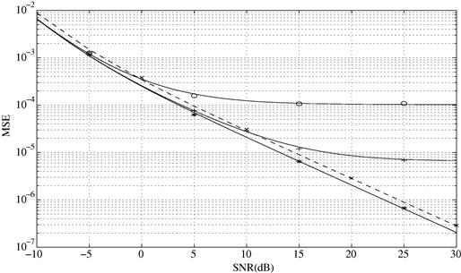
Figure 16.2 Theoretical and estimated MSE (with 500 Monte Carlo runs) of ![]() versus the SNR, for respectively white
versus the SNR, for respectively white ![]() , colored (+) and harmonic (*) signals for
, colored (+) and harmonic (*) signals for ![]() after Toeplitzation (—) and without Toeplitzation (- - -).
after Toeplitzation (—) and without Toeplitzation (- - -).
Usually, performance analyses are evaluated as a function of the number ![]() of observed snapshots without taking the sampling rate into account. In fact, depending on the value of this sampling rate, the collected samples
of observed snapshots without taking the sampling rate into account. In fact, depending on the value of this sampling rate, the collected samples ![]() are more or less temporally correlated and performance is affected. Thus, the interesting question arises as to how the asymptotic covariance of the DOA estimators (denoted here
are more or less temporally correlated and performance is affected. Thus, the interesting question arises as to how the asymptotic covariance of the DOA estimators (denoted here ![]() ) varies with this sampling rate
) varies with this sampling rate ![]() for a fixed observation interval
for a fixed observation interval ![]() . This question has been investigated in [20], in which the continuous-time noise envelope
. This question has been investigated in [20], in which the continuous-time noise envelope ![]() is spatially white and temporally white in the bandwidth
is spatially white and temporally white in the bandwidth ![]() . It has been proved:
. It has been proved:
• If the signals ![]() are oversampled (
are oversampled (![]() )
)
![]()
irrespective of the sample rate ![]() .
.
• If the signals ![]() are subsampled (
are subsampled (![]() )
)
![]()
Consequently the array must be temporally oversampled, and the parameter of interest that characterizes performance ought not to be the number ![]() of snapshots, but rather the observation interval
of snapshots, but rather the observation interval ![]() .
.
3.16.4.4 Subspace-based algorithms
We concentrate now on the family of second-order algorithms based on the orthogonal noise8 projector ![]() (16.10). These algorithms estimate
(16.10). These algorithms estimate ![]() , either by extrema-searching approaches (MUSIC, Min-Norm, etc.), by polynomial rooting approaches (Pisarenko, root MUSIC, and root Min-Norm for ULA), or by matrix shifting approaches (ESPRIT, TAM, Matrix pencil method). The most celebrated of these algorithms is the MUSIC algorithm, where
, either by extrema-searching approaches (MUSIC, Min-Norm, etc.), by polynomial rooting approaches (Pisarenko, root MUSIC, and root Min-Norm for ULA), or by matrix shifting approaches (ESPRIT, TAM, Matrix pencil method). The most celebrated of these algorithms is the MUSIC algorithm, where ![]() is estimated as the
is estimated as the ![]() deepest minima in a
deepest minima in a ![]() -dimensional (for
-dimensional (for ![]() parameters per source) of the following localization function
parameters per source) of the following localization function ![]() :
:
![]() (16.67)
(16.67)
of the so-called spatial null spectrum (or equivalently as the ![]() highest peaks (maxima) of its inverse). This algorithm has given a plethora of variants. For example, in the particular case of the ULA, this standard MUSIC algorithm have been favorably replaced by the root MUSIC algorithm. Using the general methodology presented in Section 3.16.3.1.2, the asymptotic distribution of
highest peaks (maxima) of its inverse). This algorithm has given a plethora of variants. For example, in the particular case of the ULA, this standard MUSIC algorithm have been favorably replaced by the root MUSIC algorithm. Using the general methodology presented in Section 3.16.3.1.2, the asymptotic distribution of ![]() given by any subspace-based algorithms alg is simply derived from the expression of the
given by any subspace-based algorithms alg is simply derived from the expression of the ![]() -differential matrix
-differential matrix ![]() of the mapping
of the mapping ![]() evaluated at
evaluated at ![]() . For example, for the standard MUSIC algorithm,
. For example, for the standard MUSIC algorithm, ![]() is straightforwardly obtained from the first-order expansion of
is straightforwardly obtained from the first-order expansion of ![]() that gives for one parameter per source
that gives for one parameter per source
 (16.68)
with ![]() and
and ![]() . Using (16.68) with (16.16) and (16.23) allow one to directly prove that the sequences
. Using (16.68) with (16.16) and (16.23) allow one to directly prove that the sequences ![]() converges in distribution to the zero-mean Gaussian distribution of covariance matrix given elementwise by
converges in distribution to the zero-mean Gaussian distribution of covariance matrix given elementwise by ![]() and compactly by
and compactly by
![]() (16.69)
(16.69)
where ![]() and
and ![]() has been defined in Section 3.16.3.1.2. Note that these expressions have been derived in [3] by much more involved derivations based on the asymptotic distribution of the eigenvectors of the sample covariance matrix
has been defined in Section 3.16.3.1.2. Note that these expressions have been derived in [3] by much more involved derivations based on the asymptotic distribution of the eigenvectors of the sample covariance matrix ![]() . Finally, note that if the sample orthogonal noise projector
. Finally, note that if the sample orthogonal noise projector ![]() is replaced by an adaptive estimator
is replaced by an adaptive estimator ![]() of
of ![]() , where
, where ![]() is the step-size of an arbitrary constant step-size recursive stochastic algorithm (see e.g., [72,73]), it has been proved in [72] that
is the step-size of an arbitrary constant step-size recursive stochastic algorithm (see e.g., [72,73]), it has been proved in [72] that ![]() converges in distribution to the zero-mean Gaussian distribution of covariance matrix given also by
converges in distribution to the zero-mean Gaussian distribution of covariance matrix given also by ![]() , where
, where ![]() is an adaptive estimate of
is an adaptive estimate of ![]() given by the MUSIC algorithm based on the specific adaptive estimate
given by the MUSIC algorithm based on the specific adaptive estimate ![]() of
of ![]() studied in [72]. Using a similar approach [26], it has been proved that the Root MUSIC algorithm associated with the ULA, presents the same asymptotic distribution, but slightly outperforms the standard MUSIC algorithm outside the asymptotic regime. This analysis has been extended to MUSIC-like algorithms applied to the orthogonal noise projectors
studied in [72]. Using a similar approach [26], it has been proved that the Root MUSIC algorithm associated with the ULA, presents the same asymptotic distribution, but slightly outperforms the standard MUSIC algorithm outside the asymptotic regime. This analysis has been extended to MUSIC-like algorithms applied to the orthogonal noise projectors ![]() [resp.
[resp. ![]() ] associated with the complementary sample covariance
] associated with the complementary sample covariance ![]() [the augmented sample covariance
[the augmented sample covariance ![]() ] matrices for the DOA estimation of arbitrary noncircular [resp. rectilinear] sources [27]. Finally, note that with our general methodology, all the expressions of the covariance
] matrices for the DOA estimation of arbitrary noncircular [resp. rectilinear] sources [27]. Finally, note that with our general methodology, all the expressions of the covariance ![]() can be straightforward extended for several parameter per source.
can be straightforward extended for several parameter per source.
The expression of the covariance (16.69) of the asymptotic distribution of ![]() given the standard MUSIC algorithm has been analyzed in detail (see, e.g., [2,3]). In particular it has been proved that the MUSIC algorithm is asymptotically efficient for a single source, an arbitrary number of parameters per source and
given the standard MUSIC algorithm has been analyzed in detail (see, e.g., [2,3]). In particular it has been proved that the MUSIC algorithm is asymptotically efficient for a single source, an arbitrary number of parameters per source and ![]() depending on
depending on ![]() , e.g., for one parameter per source
, e.g., for one parameter per source
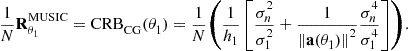
For several sources, the MUSIC algorithm is in general asymptotically inefficient, in particular for correlated sources for which the efficiency degrades when the correlation between the sources increases. The degradation of performances are considerable for highly correlated sources for any value of the SNRs. In contrast, for uncorrelated sources, the MUSIC algorithm is asymptotically efficient when ![]() tends to zero, in the following sense
tends to zero, in the following sense ![]() . So, in practice, for uncorrelated sources, the MUSIC algorithm is asymptotically efficient for high SNRs of all the sources.
. So, in practice, for uncorrelated sources, the MUSIC algorithm is asymptotically efficient for high SNRs of all the sources.
It is of utmost importance to investigate in what region of ![]() and SNR, the asymptotic theoretical results can predict actual performance. But unfortunately, only Monte Carlo simulations can specify this region. We illustrate in the following the SNR threshold region for the SML, DML, and MUSIC algorithm.
and SNR, the asymptotic theoretical results can predict actual performance. But unfortunately, only Monte Carlo simulations can specify this region. We illustrate in the following the SNR threshold region for the SML, DML, and MUSIC algorithm.
Consider two zero-mean circular Gaussian sources impinging on an ULA (16.2) with ![]() (for which the 3 dB bandwidth is about
(for which the 3 dB bandwidth is about ![]() ) and a spatially uniform white noise (16.3). The source
) and a spatially uniform white noise (16.3). The source ![]() consist of a strong direct path at
consist of a strong direct path at ![]() relative to array broadside and a weaker (multipath at
relative to array broadside and a weaker (multipath at ![]() ) at −3 dB w.r.t.
) at −3 dB w.r.t. ![]() . The correlation between
. The correlation between ![]() and
and ![]() is
is ![]() giving thus the source covariance matrix
giving thus the source covariance matrix  . Figure 16.3 shows the root mean square error (RMSE) of the estimated DOA
 ![]() by the MUSIC algorithm w.r.t. the SNR defined by
by the MUSIC algorithm w.r.t. the SNR defined by ![]() , compared with the theoretical standard deviation (TSD)
, compared with the theoretical standard deviation (TSD) ![]() and the square root of the stochastic CRB
and the square root of the stochastic CRB ![]() . We see from this figure that the MUSIC algorithm is not efficient at all for highly correlated sources. Furthermore, the domain of validity of the asymptotic regime is here very limited, i.e., for
. We see from this figure that the MUSIC algorithm is not efficient at all for highly correlated sources. Furthermore, the domain of validity of the asymptotic regime is here very limited, i.e., for ![]() , SNR > 30 dB is required.
, SNR > 30 dB is required.

Figure 16.3 RMSE of ![]() estimated by the MUSIC algorithm (averaged on 1000 runs) compared with the theoretical standard deviation and the square root of the stochastic CRB, as a function of the SNR for
estimated by the MUSIC algorithm (averaged on 1000 runs) compared with the theoretical standard deviation and the square root of the stochastic CRB, as a function of the SNR for ![]() .
.
With the same parameters, Figure 16.4 shows the RMSE of the estimated DOA ![]() by the SML and DML algorithms which are compared with the TSD
by the SML and DML algorithms which are compared with the TSD ![]() and
and ![]() and the square roots of the CRBs
and the square roots of the CRBs ![]() and
and ![]() . We see from this figure that the numerical values of the four expressions of (16.57) are very close and the performance of the two ML algorithms are very similar except for the SNR threshold region for which the SML algorithm is efficient for SNR > 0 dB with
. We see from this figure that the numerical values of the four expressions of (16.57) are very close and the performance of the two ML algorithms are very similar except for the SNR threshold region for which the SML algorithm is efficient for SNR > 0 dB with ![]() . Finally, comparing Figures 16.3 and 16.4, we see that both ML algorithms largely outperform the MUSIC algorithm for highly correlated sources.
. Finally, comparing Figures 16.3 and 16.4, we see that both ML algorithms largely outperform the MUSIC algorithm for highly correlated sources.

3.16.4.5 Robustness of algorithms
We distinguish in this subsection, the robustness of the DOA estimation algorithms w.r.t. the narrowband assumption and to array modeling errors, because for the array modeling errors, the model (16.1) remains valid with a modified steering matrix, in contrast to the violation of narrowband assumption, for which (16.1) must be modified.
3.16.4.5.1 Robustness w.r.t. the narrowband assumption
As the wideband assumption generally requires an increased computational complexity compared to the narrowband ones, it is of interest to examine if the narrowband methods can be used for a sufficiently wide bandwidth without sacrificing performance. Some responses to this question have been given in [74] for symmetric spectra w.r.t. the demodulation frequency and in [75] for non-symmetric spectra and/or offset of the centered value of the spectra w.r.t. the demodulation frequency ![]() . In these assumptions, the model (16.1) of the complex envelope of the measurements becomes
. In these assumptions, the model (16.1) of the complex envelope of the measurements becomes
 (16.70)
where ![]() (with
(with ![]() ) and
) and ![]() is the spectral measure of the
is the spectral measure of the ![]() th source. Using the general methodology explained in Section 3.16.3.1, based on a first-order expansion of the DOA estimate
th source. Using the general methodology explained in Section 3.16.3.1, based on a first-order expansion of the DOA estimate ![]() in the neighborhood of
in the neighborhood of ![]() (where
(where ![]() and
and ![]() are the orthogonal projectors onto the noise subspace associated with the covariance of (16.70) and (16.1), respectively), general closed-form expressions of the asymptotic (w.r.t. the number of snapshots and source bandwidth) for arbitrary subspace-based algorithm have been derived in [75]. It is found that the behavior of these DOA estimators strongly depends on the symmetry of the source spectra w.r.t. their centered value and on the offset of this centered value w.r.t.
are the orthogonal projectors onto the noise subspace associated with the covariance of (16.70) and (16.1), respectively), general closed-form expressions of the asymptotic (w.r.t. the number of snapshots and source bandwidth) for arbitrary subspace-based algorithm have been derived in [75]. It is found that the behavior of these DOA estimators strongly depends on the symmetry of the source spectra w.r.t. their centered value and on the offset of this centered value w.r.t. ![]() . It is showed that the narrowband SOS-based algorithms are much more sensitive to the frequency offset than to the bandwidth.
. It is showed that the narrowband SOS-based algorithms are much more sensitive to the frequency offset than to the bandwidth.
In particular for source spectra ![]() symmetric w.r.t. the demodulation frequency
symmetric w.r.t. the demodulation frequency ![]() , it is proved that the estimated DOAs given by any narrowband subpace-based algorithm are asymptotically unbiased w.r.t. the number of snapshots and signal bandwidth. More precisely
, it is proved that the estimated DOAs given by any narrowband subpace-based algorithm are asymptotically unbiased w.r.t. the number of snapshots and signal bandwidth. More precisely
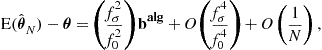
where ![]() is the definition used for the bandwidth. Furthermore, for a single source,
is the definition used for the bandwidth. Furthermore, for a single source, ![]() , where the nuisance parameters are now the terms of the Hermitian matrix
, where the nuisance parameters are now the terms of the Hermitian matrix ![]() and
and ![]() . This new parameterization allows to derive the circular Gaussian stochastic CRB issued from a non-zero bandwidth
. This new parameterization allows to derive the circular Gaussian stochastic CRB issued from a non-zero bandwidth ![]() . It is related to the standard
. It is related to the standard ![]() by the relation
by the relation

where the expression of ![]() is given in [75].
is given in [75].
3.16.4.5.2 Robustness to array modeling errors
Imprecise knowledge of the gain and phase characteristics of the array sensors, and of the sensor locations and possible mutual coupling, can seriously degrade the theoretical performance of the DOA estimation algorithms. Experimental systems attempt to eliminate or minimize these errors by careful calibrations. But even when initial calibration is possible, system parameters may change over time and thus the array modeling errors cannot be completely eliminated. Consequently, it is useful to qualify the sensitivity of the DOA estimator algorithms to these modeling errors, i.e., to study the effect of difference between the true and assumed array manifold ![]() caused by modeling errors, on DOA estimator algorithms. This analysis has received relatively little attention in the literature.
caused by modeling errors, on DOA estimator algorithms. This analysis has received relatively little attention in the literature.
In these studies, to simplify the analysis, the covariance matrix ![]() is assumed perfectly known, i.e., the effects of a finite number of samples is assumed negligible. Let
is assumed perfectly known, i.e., the effects of a finite number of samples is assumed negligible. Let ![]() gather the array parameters which are the subject of the sensitivity analysis. For example,
gather the array parameters which are the subject of the sensitivity analysis. For example, ![]() may contain the sensors gain, phases or location, or other parameters such as the mutual coupling coefficients of the array sensors. A DOA estimation algorithm uses the steering matrix
may contain the sensors gain, phases or location, or other parameters such as the mutual coupling coefficients of the array sensors. A DOA estimation algorithm uses the steering matrix ![]() , corresponding to a nominal value
, corresponding to a nominal value ![]() of the array parameters that differs from the true steering matrix
of the array parameters that differs from the true steering matrix ![]() , where
, where ![]() is slightly different from
is slightly different from ![]() (see particular parameterizations studied in [76,77]). We refer to the difference between the true and assumed array parameters as a modeling error. The sensitivity study of a particular DOA estimation algorithm consists to provide a relation between
(see particular parameterizations studied in [76,77]). We refer to the difference between the true and assumed array parameters as a modeling error. The sensitivity study of a particular DOA estimation algorithm consists to provide a relation between ![]() and the modeling error
and the modeling error ![]() in the mapping
in the mapping
![]() (16.71)
(16.71)
where naturally ![]() , if
, if ![]() denotes an arbitrary second-order algorithm based on the nominal array. Using a first order perturbation of (16.71) in the neighborhood of
denotes an arbitrary second-order algorithm based on the nominal array. Using a first order perturbation of (16.71) in the neighborhood of ![]() , through those of the orthogonal projector on the noise subspace
, through those of the orthogonal projector on the noise subspace ![]() , a relation
, a relation ![]() where
where ![]() is linear has been given for the MUSIC and DML algorithms in [77–79], respectively. These works model the errors
is linear has been given for the MUSIC and DML algorithms in [77–79], respectively. These works model the errors ![]() by zero-mean independent random variables (
by zero-mean independent random variables (![]() where
where ![]() is a random vector whose elements are zero-mean unit variance random variables). They lead to estimates that are approximatively unbiased (i.e.,
is a random vector whose elements are zero-mean unit variance random variables). They lead to estimates that are approximatively unbiased (i.e., ![]() ) and where their approximative variances depend only on the second-order statistics of the modeling errors (more precisely
) and where their approximative variances depend only on the second-order statistics of the modeling errors (more precisely ![]() ,
, ![]() ). However, by confronting these theoretical results with numerical experiments, one notices that the MUSIC and DML algorithms are biased in the presence of multiple sources and these theoretic and experimental variances do not agree with larger modeling errors. More precisely, these theoretical results are valid only up to the point where the probability of resolution is close to one (see [25]).
). However, by confronting these theoretical results with numerical experiments, one notices that the MUSIC and DML algorithms are biased in the presence of multiple sources and these theoretic and experimental variances do not agree with larger modeling errors. More precisely, these theoretical results are valid only up to the point where the probability of resolution is close to one (see [25]).
To take into account these larger modeling errors, a more accurate relation between ![]() and
and ![]() , based on a second-order expansion of
, based on a second-order expansion of ![]() around
around ![]() (provided by a recursive
(provided by a recursive ![]() th order expansion of
th order expansion of ![]() w.r.t.
w.r.t. ![]() [6]) as been given in [25,80] for analyzing the sensitivity of the MUSIC and DML algorithms to larger modeling errors. Modeling the errors
[6]) as been given in [25,80] for analyzing the sensitivity of the MUSIC and DML algorithms to larger modeling errors. Modeling the errors ![]() as previously, an approximation of the bias
as previously, an approximation of the bias ![]() that depends on the second-order statistics of the modeling errors, and of the variance that now depends on the fourth-order statistics of the modeling errors, are given. These refined closed-form expressions can predict the actual performance observed by numerical experiments for larger modeling errors, in particular in the threshold regions of the MUSIC and DML algorithms.
that depends on the second-order statistics of the modeling errors, and of the variance that now depends on the fourth-order statistics of the modeling errors, are given. These refined closed-form expressions can predict the actual performance observed by numerical experiments for larger modeling errors, in particular in the threshold regions of the MUSIC and DML algorithms.
Note that the sensitivity of DOA estimators to modeling errors of the noise covariance matrix, that includes the presence of undetected weak signals, has also been studied in the literature (see, e.g., [81]). Finally, note that the combined effects of random array modeling errors and finite samples have been analyzed for the class of so-called signal subspace fitting (SSF) algorithms in [82]. In addition to deriving the first-order asymptotic expressions for the covariance of the estimation error, an additional weighting matrix has been introduced in (16.61) that has been optimized for any particular random array modeling errors.
3.16.4.6 High-order algorithms
When the sources are non Gaussian distributed, they convey valuable statistical information in their moments of order greater than two (this is in particular true when considering communications signals). In these circumstances, it makes sense to consider DOA estimation techniques using this higher order information. Of particular interest are the algorithms based on higher order cumulants of the measurements ![]() due to their additivity property in the sums of independent components. Furthermore, these cumulants show the distinctive property of being in a certain sense, insensitive to additive Gaussian noise, making it possible to devise consistent DOA estimates without it being necessary to know, to model or to estimate the noise covariance
due to their additivity property in the sums of independent components. Furthermore, these cumulants show the distinctive property of being in a certain sense, insensitive to additive Gaussian noise, making it possible to devise consistent DOA estimates without it being necessary to know, to model or to estimate the noise covariance ![]() . As generally, the distributions of the sources are even, their odd order moments are zero and thus to cope with these signals, only the even high-order cumulants of the measurements are used.
. As generally, the distributions of the sources are even, their odd order moments are zero and thus to cope with these signals, only the even high-order cumulants of the measurements are used.
Computational considerations dictate using mainly fourth-order cumulants. To use these approaches, we consider the assumptions of Section 3.16.2.2, in which we add that the sources ![]() have nonvanishing fourth-order cumulants. Furthermore, we assume that their moments are finite up to the eighth-order, to study the statistical performance of these algorithms.
have nonvanishing fourth-order cumulants. Furthermore, we assume that their moments are finite up to the eighth-order, to study the statistical performance of these algorithms.
Of course, there are many more quadruples than pairs of indices, and consequently a very large number of cumulants ![]() ,
, ![]() for circular sources (and more,
for circular sources (and more, ![]() and
and ![]() ,
, ![]() for noncircular sources) can be exploited despite their redundancies, to identify the DOA parameters with unknown noise covariance. For example, for circular signals, the maximum set of nonredundant cumulants is
for noncircular sources) can be exploited despite their redundancies, to identify the DOA parameters with unknown noise covariance. For example, for circular signals, the maximum set of nonredundant cumulants is
![]()
The asymptotically minimum variance (AMV) algorithm (see Section 3.16.3.3) based on a subset of fourth-order cumulants that can identify the DOA parameters, is the nonlinear least square algorithm (16.40) in which ![]() gathers the involved cumulants. To implement this AMV algorithm, one has to decide which cumulants should be included in
gathers the involved cumulants. To implement this AMV algorithm, one has to decide which cumulants should be included in ![]() . The best estimate would be obtained when all nonredundant cumulants are selected. This, however, may require excessive computations if
. The best estimate would be obtained when all nonredundant cumulants are selected. This, however, may require excessive computations if ![]() is large. However it is sufficient to deal with a reduced set of cumulants, although there do not seem to be any simple guidelines in this matter [60]. In practice, a good tradeoff between computational complexity and accuracy is to devise suboptimal algorithms that require an overall computational effort similar to the second-order algorithms, while retaining a fourth-order cumulants subset, sufficient for DOA indentification. Such algorithms have been proposed in the literature such as the diagonal slice (DS), the contracted quadricovariance (CQ) and the so called 4-MUSIC [60] algorithms. The first two algorithms are fourth-order subspace-based algorithms built on the following rank defective
is large. However it is sufficient to deal with a reduced set of cumulants, although there do not seem to be any simple guidelines in this matter [60]. In practice, a good tradeoff between computational complexity and accuracy is to devise suboptimal algorithms that require an overall computational effort similar to the second-order algorithms, while retaining a fourth-order cumulants subset, sufficient for DOA indentification. Such algorithms have been proposed in the literature such as the diagonal slice (DS), the contracted quadricovariance (CQ) and the so called 4-MUSIC [60] algorithms. The first two algorithms are fourth-order subspace-based algorithms built on the following rank defective ![]() matrices:
matrices:
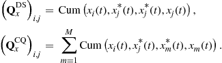
They require ![]() sources and their statistical performance has been analyzed in [19] with the general framework explained in Section 3.16.3.1. In particular, it is has been proved that for a single source and a ULA in spatially uniform white noise, these two fourth-order algorithms have similar performance to the MUSIC algorithm, except for low SNR, for which the MUSIC algorithm outperforms both fourth-order algorithms. The 4-MUSIC algorithm is built from the rank defective
sources and their statistical performance has been analyzed in [19] with the general framework explained in Section 3.16.3.1. In particular, it is has been proved that for a single source and a ULA in spatially uniform white noise, these two fourth-order algorithms have similar performance to the MUSIC algorithm, except for low SNR, for which the MUSIC algorithm outperforms both fourth-order algorithms. The 4-MUSIC algorithm is built from the rank defective ![]() matrix
matrix
![]()
It is proved in [60] that
![]()
where ![]() ,
, ![]() .
. ![]() is indefinite in general and its rank is
is indefinite in general and its rank is ![]() where the
where the ![]() sources are divided in
sources are divided in ![]() groups, with
groups, with ![]() in the
in the ![]() th group. The sources in each group are assumed to be dependent, while sources belonging to different groups are assumed independent. Because the vectors
th group. The sources in each group are assumed to be dependent, while sources belonging to different groups are assumed independent. Because the vectors ![]() ,
, ![]() are
are ![]() columns of
columns of ![]() , the 4-MUSIC algorithm is obtained by searching the
, the 4-MUSIC algorithm is obtained by searching the ![]() deepest minima of the following localization function
deepest minima of the following localization function ![]() :
:
![]() (16.72)
(16.72)
where ![]() is now, the orthogonal projector onto the noise subspace of the sample estimate
is now, the orthogonal projector onto the noise subspace of the sample estimate ![]() of
of ![]() . In practice the statistical dependence of the sources are unknown. Porat and Fiedlander [60] has proposed to retain only
. In practice the statistical dependence of the sources are unknown. Porat and Fiedlander [60] has proposed to retain only ![]() , rather
, rather ![]() eigenvectors corresponding to the smallest singular values of
eigenvectors corresponding to the smallest singular values of ![]() . We note that, to the best of our knowledge, no complete statistical performance analysis of this algorithm has yet appeared in the literature. Despite its higher variance (w.r.t. the MUSIC algorithm under the assumption of spatially uniform white noise), this fourth-order algorithm presents some advantages, aside from its capacity to deal with unknown Gaussian noise fields. Using the concept of virtual array, it is proved in [83] that this algorithm can identify up to
. We note that, to the best of our knowledge, no complete statistical performance analysis of this algorithm has yet appeared in the literature. Despite its higher variance (w.r.t. the MUSIC algorithm under the assumption of spatially uniform white noise), this fourth-order algorithm presents some advantages, aside from its capacity to deal with unknown Gaussian noise fields. Using the concept of virtual array, it is proved in [83] that this algorithm can identify up to ![]() sources when the sensors are identical and up to
sources when the sensors are identical and up to ![]() sources for different sensors. Furthermore, it is shown that its resolution for closely spaced sources and robustness to modeling errors is improved with respect to the MUSIC algorithm. To increase even more its number of sources to be processed, resolution and robustness to modeling errors, extensions of this 4-MUSIC algorithms, giving rise to the 2
sources for different sensors. Furthermore, it is shown that its resolution for closely spaced sources and robustness to modeling errors is improved with respect to the MUSIC algorithm. To increase even more its number of sources to be processed, resolution and robustness to modeling errors, extensions of this 4-MUSIC algorithms, giving rise to the 2![]() -MUSIC (with
-MUSIC (with ![]() ) has been proposed [84].
) has been proposed [84].
3.16.5 Detection of number of sources
One of the more difficult and critical problems facing passive sensor arrays systems is the detection of the number ![]() of sources impinging on the array. This is a key step in most of the parametric estimation techniques that were briefly described in Section 3.16.4. The eigendecomposition based techniques require in addition, information on the dimension
of sources impinging on the array. This is a key step in most of the parametric estimation techniques that were briefly described in Section 3.16.4. The eigendecomposition based techniques require in addition, information on the dimension ![]() of the signal subspace. If the source covariance
of the signal subspace. If the source covariance ![]() has full rank, i.e., there are no coherent sources present,
has full rank, i.e., there are no coherent sources present, ![]() and
and ![]() are identical. Moreover, the solution of the detection problem has, in many cases, value of its own, regardless of the DOA estimation problem.
are identical. Moreover, the solution of the detection problem has, in many cases, value of its own, regardless of the DOA estimation problem.
A natural scheme for detecting the number ![]() of sources is to formulate a likelihood ratio test based on the SML estimator (16.49). Such a test is often referred to as a generalized likelihood ratio test (GLRT). This test can be implemented by a sequential test procedure (see, e.g., [12, Sec. 4.7.1]). For each hypothesis, the likelihood ratio statistic is computed and compared to a threshold. The accepted hypothesis is the first one for which the threshold is crossed. The problem with this method is the subjective judgment required for deciding on the threshold levels or the associated probabilities of false alarm related by the asymptotic distribution of the normalized likelihood ratio.
of sources is to formulate a likelihood ratio test based on the SML estimator (16.49). Such a test is often referred to as a generalized likelihood ratio test (GLRT). This test can be implemented by a sequential test procedure (see, e.g., [12, Sec. 4.7.1]). For each hypothesis, the likelihood ratio statistic is computed and compared to a threshold. The accepted hypothesis is the first one for which the threshold is crossed. The problem with this method is the subjective judgment required for deciding on the threshold levels or the associated probabilities of false alarm related by the asymptotic distribution of the normalized likelihood ratio.
Another important approach to the detection problem is the application of the information theoretic criteria for model selection. Unlike the conventional hypothesis testing based approaches, these criteria do not require any subjective threshold setting. Among them, the minimum description length (MDL) criterion introduced by Rissanen [85] is the most widely used because of its consistency. This technique has been used for detecting the signal subspace dimension ![]() [13], and also for detecting the number of sources
[13], and also for detecting the number of sources ![]() [86]. We concentrate now on the detection of
[86]. We concentrate now on the detection of ![]() .
.
3.16.5.1 MDL criterion
The information theoretic criteria approach is a general method for detecting the order ![]() of a statistical model. That is, given a parameterized probability density function
of a statistical model. That is, given a parameterized probability density function ![]() for various order
for various order ![]() , detect
, detect ![]() such that
such that ![]() , where
, where ![]() is the ML estimate of
is the ML estimate of ![]() and
and ![]() is a penalty function. For the MDL criterion which is based on a particular penalty function,
is a penalty function. For the MDL criterion which is based on a particular penalty function, ![]() is given for
is given for ![]() independent identically distributed measurements
independent identically distributed measurements ![]() , by
, by
![]() (16.73)
(16.73)
where ![]() denotes the number of free real-valued parameters in
denotes the number of free real-valued parameters in ![]() . Depending on the distribution of the measurements
. Depending on the distribution of the measurements ![]() and its parametrization
and its parametrization ![]() , different implementations of the MDL criterion have been proposed.
, different implementations of the MDL criterion have been proposed.
The most often used assumption, is the zero-mean circular Gaussian distribution associated with the parametrization (16.1) in which all the elements of the steering matrix ![]() are assumed unknown with the only restriction that
are assumed unknown with the only restriction that ![]() has full column rank with
has full column rank with ![]() . For this modeling, the measurements can be parameterized by the parameter
. For this modeling, the measurements can be parameterized by the parameter
![]()
where ![]() are the eigenvalues of
are the eigenvalues of ![]() and
and ![]() ,…,
,…,![]() , the eigenvectors associated with the largest
, the eigenvectors associated with the largest ![]() eigenvalues, and the general MDL criterion (16.73), which is referred to as the Gaussian MDL (GMDL), becomes [13]
eigenvalues, and the general MDL criterion (16.73), which is referred to as the Gaussian MDL (GMDL), becomes [13]
![]() (16.74)
(16.74)
with ![]() and
and ![]() , where
, where ![]() are the eigenvalues of the sample covariance matrix
are the eigenvalues of the sample covariance matrix ![]() , denoted here by
, denoted here by ![]() .
.
3.16.5.2 Performance analysis of MDL criterion
This GMDL criterion has been analyzed in [16], and it has been shown to be a consistent estimator of the rank ![]() , i.e., the probability of error decreases to zero as the number
, i.e., the probability of error decreases to zero as the number ![]() of measurements increases to infinity. Moreover, under mild regularity conditions, like finite second moments, it is a consistent estimator of the rank
of measurements increases to infinity. Moreover, under mild regularity conditions, like finite second moments, it is a consistent estimator of the rank ![]() , even if the measurements are non-Gaussian. This property contrasts with the Akaike information criterion (AIC) that yields an inconsistent estimate of that tends, asymptotically, to overestimate
, even if the measurements are non-Gaussian. This property contrasts with the Akaike information criterion (AIC) that yields an inconsistent estimate of that tends, asymptotically, to overestimate ![]() [13].
[13].
The GMDL criterion has been further analyzed by considering the events ![]() and
and ![]() , called underestimation and overestimation, respectively. Since
, called underestimation and overestimation, respectively. Since ![]() are functions of the eigenvalues
are functions of the eigenvalues ![]() of
of ![]() , the derivation of the probabilities
, the derivation of the probabilities ![]() and
and ![]() needs the joint exact or asymptotic distribution of
needs the joint exact or asymptotic distribution of ![]() . This asymptotic distribution is available for circular complex Gaussian distribution [87] and more generally for arbitrary distributions with finite fourth-order moments [14], but unfortunately, the functional
. This asymptotic distribution is available for circular complex Gaussian distribution [87] and more generally for arbitrary distributions with finite fourth-order moments [14], but unfortunately, the functional ![]() (16.74) is too complicated to infer its asymptotically distribution. Therefore, for simplifying the derivation of these probabilities, it has been argued [36,88,89] by extended Monte Carlo experiments (essentially for
(16.74) is too complicated to infer its asymptotically distribution. Therefore, for simplifying the derivation of these probabilities, it has been argued [36,88,89] by extended Monte Carlo experiments (essentially for ![]() and
and ![]() ) that
) that
![]() (16.75)
(16.75)
As the probability of overestimation is concerned, exact and approximate asymptotic upper bound of this probability have been derived in [36] showing that generally ![]() . Therefore, only the probability of underestimation has been analyzed by many authors. In particular, using the refinement introduced by [90]
. Therefore, only the probability of underestimation has been analyzed by many authors. In particular, using the refinement introduced by [90]
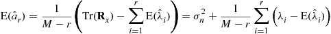
of the classical approximation ![]() and the asymptotic bias (16.18) and covariance (16.19), a closed-form expression of the probability of underestimation given by the GMDL criterion, used under arbitrary distributions with finite fourth-order moments, has been given in [14]. This expression has been analyzed for
and the asymptotic bias (16.18) and covariance (16.19), a closed-form expression of the probability of underestimation given by the GMDL criterion, used under arbitrary distributions with finite fourth-order moments, has been given in [14]. This expression has been analyzed for ![]() and
and ![]() for different distributions of the sources in [14]. Figure 16.5 illustrates the robustness of the MDL criterion to the distribution of the sources. We see from this figure that the probability of underestimation is sensitive to the distribution of the source, particularly for sources of large kurtosis and for weak values of the number
for different distributions of the sources in [14]. Figure 16.5 illustrates the robustness of the MDL criterion to the distribution of the sources. We see from this figure that the probability of underestimation is sensitive to the distribution of the source, particularly for sources of large kurtosis and for weak values of the number ![]() of snapshots.
of snapshots.

Figure 16.5 ![]() as a function of the SNR for four distributions of the source (the impulsive takes the values
as a function of the SNR for four distributions of the source (the impulsive takes the values ![]() ) with
) with ![]() and two values of the number
and two values of the number ![]() of snapshots, for an ULA with five sensors.
of snapshots, for an ULA with five sensors.
The general MDL criterion has been studied in [15], where using the approximation (16.75), a general analytical expression of ![]() has been given. This expression allows one to prove the consistency of the general MDL criterion when the number of snapshots tends to infinite and has been specialized to particular parameterized distributions. Among them, the Gaussian assumption associated with a parameterized steering matrix
has been given. This expression allows one to prove the consistency of the general MDL criterion when the number of snapshots tends to infinite and has been specialized to particular parameterized distributions. Among them, the Gaussian assumption associated with a parameterized steering matrix ![]() has been studied and some numerical illustrations show that the use of this prior information about the array geometry enables an improvement in performance of about 2 dB. Finally, note that the MDL criterion generally fails when the sample size is smaller than the number of sensors. In this situation a sample eigenvalue based detector has been proposed in [91].
has been studied and some numerical illustrations show that the use of this prior information about the array geometry enables an improvement in performance of about 2 dB. Finally, note that the MDL criterion generally fails when the sample size is smaller than the number of sensors. In this situation a sample eigenvalue based detector has been proposed in [91].
3.16.6 Resolution of two closely spaced sources
An important measure to quantify the statistical performance for the DOA estimation problem is the resolvability of closely spaced signals in terms of their parameters of interest. The principal question to characterize this resolvability is to find the minimum SNR (denoted threshold array SNR (ASNR)) required for a sensor array to correctly resolve two closely spaced signals for a given DOA distance ![]() (called angular resolution limit (ARL) or statistical resolution limit) between them. Generally in the literature they are three different ways to describe this resolution limit. The first one is based on the mean null spectrum concerning a specific algorithm. The second one is based on the estimation accuracy, more precisely on the Cramer-Rao Bound. The last one is based on the detection theory using the hypothesis test formulation.
(called angular resolution limit (ARL) or statistical resolution limit) between them. Generally in the literature they are three different ways to describe this resolution limit. The first one is based on the mean null spectrum concerning a specific algorithm. The second one is based on the estimation accuracy, more precisely on the Cramer-Rao Bound. The last one is based on the detection theory using the hypothesis test formulation.
3.16.6.1 Angular resolution limit based on mean null spectra
Based on the array beam-pattern ![]() , different resolution criteria have been defined from its main lobe w.r.t. a look direction
, different resolution criteria have been defined from its main lobe w.r.t. a look direction ![]() , as the celebrated Rayleigh resolutions such as the half power beamwidth or the null to null beamwidth that depends solely on the antenna geometry, and consequently have the serious shortcoming of being independent of the SNR.
, as the celebrated Rayleigh resolutions such as the half power beamwidth or the null to null beamwidth that depends solely on the antenna geometry, and consequently have the serious shortcoming of being independent of the SNR.
For specific so-called high resolution algorithms, such as different MUSIC-like algorithms, based on the search for two local minima of sample null spectra ![]() , two main criteria based on the mean null spectrum
, two main criteria based on the mean null spectrum ![]() have been defined. These criteria are justified by the property that the standard deviation
have been defined. These criteria are justified by the property that the standard deviation ![]() of the sample null spectrum associated with the conventional MUSIC and Min-Norm algorithms is small compared to its mean value
of the sample null spectrum associated with the conventional MUSIC and Min-Norm algorithms is small compared to its mean value ![]() in the vicinity of the true DOAs for
in the vicinity of the true DOAs for ![]() for arbitrary SNR [1].
for arbitrary SNR [1].
For the first criterion, introduced by Cox [92], two sources are resolved if the midpoint mean null spectrum is greater than the mean null spectrum in the two true source DOAs:
![]()
This criterion was first studied by Kaveh and Barabell [1] and Kaveh and Wang [93] in the resolution analysis of the conventional MUSIC and Min-Norm algorithms for two uncorrelated equal-powered sources and a ULA. This analysis has been extended to more general classes of situations, e.g., for two correlated or coherent equal-powered sources with the smoothed MUSIC algorithm [94], then for two unequal-powered sources impinging on an arbitrary array with the conventional and beamspace MUSIC algorithm [95]. A subsequent paper by Zhou et al. [96] developed a resolution measure based on the mean null spectrum and compared their results to Kaveh and Barabell’s work.
For the second criterion, introduced by Sharman and Durrani [97] and then studied by Forster and Villier [26] in the context of the conventional MUSIC and Min-Norm algorithms for two uncorrelated equal-powered sources and a ULA, two sources are resolved if the second derivative of the mean null spectrum at the midpoint is negative
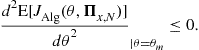
Resorting to an analysis based on perturbations of the noise projector ![]() [6], instead of those of the eigenvectors (e.g., [1,95]), these two criteria have been studied for arbitrary distributions of the sources, for the conventional MUSIC algorithm. The following closed-form expressions of the approximation of the threshold ASNR given by these two criteria have been obtained in [27]:
[6], instead of those of the eigenvectors (e.g., [1,95]), these two criteria have been studied for arbitrary distributions of the sources, for the conventional MUSIC algorithm. The following closed-form expressions of the approximation of the threshold ASNR given by these two criteria have been obtained in [27]:
 (16.76)
where ![]() and
and ![]() are fractional expressions in
are fractional expressions in ![]() specified in [27] for ULAs. These expressions (16.76) have been extended in [27] to a noncircular MUSIC algorithm adapted to rectilinear signals, introduced and analyzed in [98], for which (16.76) becomes
specified in [27] for ULAs. These expressions (16.76) have been extended in [27] to a noncircular MUSIC algorithm adapted to rectilinear signals, introduced and analyzed in [98], for which (16.76) becomes
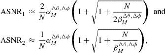 (16.77)
where ![]() is the second-order noncircularity phase separation (16.8) and where now
is the second-order noncircularity phase separation (16.8) and where now ![]() and
and ![]() are expansions of
are expansions of ![]() without constant term, whose coefficients depend on
without constant term, whose coefficients depend on ![]() ,
, ![]() and the array configuration. Closed-form expressions of
and the array configuration. Closed-form expressions of ![]() and
and ![]() are given in [27] for weak and large second-order noncircularity phase separations and ULAs, where it is proved that
are given in [27] for weak and large second-order noncircularity phase separations and ULAs, where it is proved that ![]() and
and ![]() are decreasing functions of
are decreasing functions of ![]() and thus are minimum for
and thus are minimum for ![]() .
.
Figure 16.6 illustrates these two threshold ASNRs for two independent equal-powered BPSK modulated signals impinging on a ULA with ![]() and
and ![]() . We clearly see in this figure that the noncircular MUSIC algorithm outperforms the conventional MUSIC algorithm except for very weak second-order noncircularity phase separations or which the ASNR thresholds of these two algorithms are very similar. Furthermore, we note that the behaviors of the ASNR threshold given by the two criteria are very similar although the ASNR thresholds are slightly weaker for the Sharman and Durrani criterion than for the Cox criterion.
. We clearly see in this figure that the noncircular MUSIC algorithm outperforms the conventional MUSIC algorithm except for very weak second-order noncircularity phase separations or which the ASNR thresholds of these two algorithms are very similar. Furthermore, we note that the behaviors of the ASNR threshold given by the two criteria are very similar although the ASNR thresholds are slightly weaker for the Sharman and Durrani criterion than for the Cox criterion.

Figure 16.6 Comparison of the threshold ASNRs given by the Cox (a) and Sharman and Durrani (b) criteria as a function of the DOA separation ![]() associated with the conventional MUSIC (—) and noncircular MUSIC algorithms (- -) for three values of the second-order noncircularity phase separation
associated with the conventional MUSIC (—) and noncircular MUSIC algorithms (- -) for three values of the second-order noncircularity phase separation ![]() .
.
Moreover, several authors have considered (e.g., [99–101]) the probability of resolution or an approximation of it, based on the Cox criterion applied to the null sample spectrum to circumvent the possible misleading results given by these two criteria. Finally note that the resolution capability of the conventional and Capon beamforming algorithms have been thoroughly analyzed (see, e.g., [102]). Thanks to the simple expression of their spatial null spectra (16.46), it is possible to derive an approximation of the probability of resolution defined as the probability that the dip in midway between the two sources is at least 3-dB less than the peak of either source as a function of the SNR and DOA separation. Thus, fixing a specific high confidence level, this allows one to predict the SNR required to resolve two closely spaced sources. The superiority of the Capon algorithm is proved in [102], as the resolving power increases with SNR; in contrast, the Bartlett algorithm cannot exceed the Fourier/Rayleigh limit no matter how strong the signals.
3.16.6.2 Angular resolution limit based on the CRB
Array resolution has been studied independently of any algorithm by using the CRB. Based on the observation that the standard MUSIC algorithm is unlikely to resolve closely spaced signals if the standard deviation of the DOA estimates exceed ![]() [3], Lee [103] has proposed to define the resolution limit as the DOA separation
[3], Lee [103] has proposed to define the resolution limit as the DOA separation ![]() for which
for which
![]() (16.78)
(16.78)
for the two closely spaced sources, where ![]() is somewhat arbitrarily chosen. This criterion ignores the coupling between the estimates
is somewhat arbitrarily chosen. This criterion ignores the coupling between the estimates ![]() and
and ![]() . To overcome these drawbacks, Smith has proposed [18] to define the resolution limit as the source separation that equals the square root of its own CRB, i.e.,
. To overcome these drawbacks, Smith has proposed [18] to define the resolution limit as the source separation that equals the square root of its own CRB, i.e.,
![]() (16.79)
(16.79)
with ![]() .9 This means that the angular resolution limit or the threshold ASNR are obtained by resolving the implicit equations (16.78) and (16.79). This latter criterion has been applied to the deterministic modeling of the sources in [18] and then extended to multiple parameters per source in [104]. For the stochastic modeling of the sources, the circular Gaussian distribution has been compared to the discrete one in [105]. In particular it has been proved that the threshold ASNR is inversely proportional to the number
.9 This means that the angular resolution limit or the threshold ASNR are obtained by resolving the implicit equations (16.78) and (16.79). This latter criterion has been applied to the deterministic modeling of the sources in [18] and then extended to multiple parameters per source in [104]. For the stochastic modeling of the sources, the circular Gaussian distribution has been compared to the discrete one in [105]. In particular it has been proved that the threshold ASNR is inversely proportional to the number ![]() of snapshots and to the square of
of snapshots and to the square of ![]() for the Gaussian case, in contrast to BPSK, MSK and QPSK case, for which it is inversely proportional to the fourth power of
for the Gaussian case, in contrast to BPSK, MSK and QPSK case, for which it is inversely proportional to the fourth power of ![]() .
.
3.16.6.3 Angular resolution limit based on the detection theory
The previous two approaches to characterize the angular resolution have in fact two different purposes. The first one studies the capability of a specific algorithm to estimate the DOAs of two closely spaced sources when the number of sources is known. In contrast, the second one is aiming to define an absolute limit on resolution that depends only of the array configuration and parameters of interest as the number ![]() of sensors and SNR. But this latter approach based on the ad hoc relationships (16.78) and (16.79), essentially makes sense because the CRB indicates the parameter estimation accuracy and intuitively should be related to the resolution limit. But it suffers from two drawbacks. First, the resolution limit defined by this approach is not rigorously grounded in a statistical setting. Second, if the resolution limit is expressible by (16.78) or (16.79), can the translation factor
of sensors and SNR. But this latter approach based on the ad hoc relationships (16.78) and (16.79), essentially makes sense because the CRB indicates the parameter estimation accuracy and intuitively should be related to the resolution limit. But it suffers from two drawbacks. First, the resolution limit defined by this approach is not rigorously grounded in a statistical setting. Second, if the resolution limit is expressible by (16.78) or (16.79), can the translation factor ![]() , be analytically determined?
, be analytically determined?
To solve these two problems, Liu and Nehorai have proposed to use a hypothesis test formulation [17]. This approach has been introduced in a 3D reference frame, but to be consistent with the notations of this section, it is briefly summarized in the following in the 2D framework, where the DOA of a source is the parameter ![]() . As the source localization accuracy may vary at different DOAs, consider the resolution limit at a specific DOA of interest. More precisely, assume there exists a source at a known DOA
. As the source localization accuracy may vary at different DOAs, consider the resolution limit at a specific DOA of interest. More precisely, assume there exists a source at a known DOA ![]() and we are interested in the minimum angular separation
and we are interested in the minimum angular separation ![]() that the array can resolve between this source at
that the array can resolve between this source at ![]() and another source at a direction
and another source at a direction ![]() close to
close to ![]() . Quite naturally, the resolution of the two sources can be achieved through the binary composite hypothesis test
. Quite naturally, the resolution of the two sources can be achieved through the binary composite hypothesis test
![]()
To rigorously define the resolution limit ![]() , we fix the values of
, we fix the values of ![]() and
and ![]() for this test. Otherwise,
for this test. Otherwise, ![]() could be arbitrary low, while the result of the test may be meaningless. Let
could be arbitrary low, while the result of the test may be meaningless. Let ![]() be the unknown parameter of our statistical model, where
be the unknown parameter of our statistical model, where ![]() is the parameter of interest and
is the parameter of interest and ![]() gathers all the unknown nuisance parameters. To conduct this test, the GLRT is considered due to the unknown nuisance parameters:
gathers all the unknown nuisance parameters. To conduct this test, the GLRT is considered due to the unknown nuisance parameters:
![]() (16.80)
(16.80)
where ![]() and
and ![]() denote the probability density function of the measurement
denote the probability density function of the measurement ![]() under the hypothesis
under the hypothesis ![]() and
and ![]() , respectively.
, respectively. ![]() and
and ![]() are respectively the ML estimate of
are respectively the ML estimate of ![]() and
and ![]() under
under ![]() , and
, and ![]() is the ML estimate of
is the ML estimate of ![]() under
under ![]() . The distribution of this GLRT
. The distribution of this GLRT ![]() is generally very involved to derive, but hopefully, approximations of the distribution of
is generally very involved to derive, but hopefully, approximations of the distribution of ![]() for large values of
for large values of ![]() are available under
are available under ![]() and
and ![]() . First, under
. First, under ![]() , Wilk’s theorem with nuisance parameters (see, e.g., [106, p. 132]) can be applied without having to know the exact form of
, Wilk’s theorem with nuisance parameters (see, e.g., [106, p. 132]) can be applied without having to know the exact form of ![]() . This theorem states the following convergence in distribution when
. This theorem states the following convergence in distribution when ![]() tends to
tends to ![]() :
:
![]() (16.81)
(16.81)
where ![]() denotes the central chi-square distribution with one degree of freedom (associated with the single parameter
denotes the central chi-square distribution with one degree of freedom (associated with the single parameter ![]() ). Under
). Under ![]() , the derivation of the asymptotic distribution of
, the derivation of the asymptotic distribution of ![]() is much more involved. Using a theoretical result by Stroud [107], Stuart et al. [108, Chapter 14.7] have stated that when
is much more involved. Using a theoretical result by Stroud [107], Stuart et al. [108, Chapter 14.7] have stated that when ![]() can take values10 near
can take values10 near ![]() ,
, ![]() is approximately distributed11 as
is approximately distributed11 as
![]() (16.82)
(16.82)
where ![]() denotes the noncentral chi-squared distribution with one degree of freedom and noncentrality parameter
denotes the noncentral chi-squared distribution with one degree of freedom and noncentrality parameter ![]() given by (see [109, Section 6.5])
given by (see [109, Section 6.5])
![]() (16.83)
(16.83)
whose dependence on ![]() in the FIM of
in the FIM of ![]() is emphasized, and where
is emphasized, and where ![]() denotes the (1,1) th entry of
denotes the (1,1) th entry of ![]() . It is further shown [109, Appendix 6C] that as
. It is further shown [109, Appendix 6C] that as ![]() is large, (16.83) is approximated by
is large, (16.83) is approximated by
![]() (16.84)
(16.84)
Based on these limit and approximate distributions of ![]() under
under ![]() and
and ![]() for which the GLRT in (16.81) can be rewritten as
for which the GLRT in (16.81) can be rewritten as
![]() (16.85)
(16.85)
the angular resolution limit (ARL) has been computed in [17] by using the two constraints
![]()
where the values of ![]() and
and ![]() are fixed and where
are fixed and where ![]() and
and ![]() denote the right tail probability of the
denote the right tail probability of the ![]() and
and ![]() distributions, respectively. It assumes the form
distributions, respectively. It assumes the form
![]()
where the factor ![]() is analytically determined by the preassigned values of
is analytically determined by the preassigned values of ![]() and
and ![]() . Note that the SNR is embedded in the expression of CRB
. Note that the SNR is embedded in the expression of CRB![]() that is proportional to
that is proportional to ![]() . The dependence on the SNR of the CRB may vary according to the distribution of the sources. For example, Delmas and Abeida [105] proves that the CRB of the DOA separation of discrete sources is very different from those of Gaussian sources.
. The dependence on the SNR of the CRB may vary according to the distribution of the sources. For example, Delmas and Abeida [105] proves that the CRB of the DOA separation of discrete sources is very different from those of Gaussian sources.
References
1. Kaveh M, Barabell AJ. The statistical performance of the MUSIC and the Minimum-Norm algorithms in resolving plane waves in noise. IEEE Trans ASSP. 1986;34(2):331–341.
2. Porat B, Friedlander B. Analysis of the asymptotic relative efficiency of the MUSIC algorithm. IEEE Trans ASSP. 1988;36(4):532–544.
3. Stoica P, Nehorai A. MUSIC, maximum likelihood, and Cramer-Rao bound. IEEE Trans ASSP. 1989;37(5):720–741.
4. Stoica P, Nehorai A. MUSIC, maximum likelihood, and Cramer-Rao bound: further results and comparisons. IEEE Trans ASSP. 1990;38(12):2140–2150.
5. Xu W, Buckley KM. Bias analysis of the MUSIC location estimator. IEEE Trans Signal Process. 1992;40(10):2559–2569.
6. Krim H, Forster P, Proakis G. Operator approach to performance analysis of root-MUSIC and root-min-norm. IEEE Trans Signal Process. 1992;40(7):1687–1696.
7. Gorokhov A, Abramovich Y, Böhme JF. Unified analysis of DOA estimation algorithms for covariance matrix transforms. Signal Process. 1996;55:107–115.
8. Li F, Vaccaro RJ. Unified analysis for DOA estimation algorithms in array signal processing. Signal Process. 1991;25(2):147–169.
9. Li F, Liu H, Vaccaro RJ. Performance analysis for DOA estimation algorithms: unification, simplification, and observations. IEEE Trans Aerosp Electron Syst. 1993;29(4):1170–1184.
10. Ottersten B, Viberg M, Kailath T. Analysis of subspace fitting and ML techniques for parameter estimation from sensor array data. IEEE Trans Signal Process. 1992;40(3):590–599.
11. Stoica P, Nehorai A. Performance study of conditional and unconditional direction of arrival estimation. IEEE Trans ASSP. 1990;38(10):1783–1795.
12. Ottersten B, Viberg M, Stoica P, Nehorai A. Exact and large sample maximum likelihood techniques for parameter estimation and detection in array processing. In: Haykin S, Litva J, Shepherd TJ, eds. Radar Array Processing. Berlin: Springer-Verlag; 1993;99–151.
13. Wax M, Kailath T. Detection of signals by information theoretic criteria. IEEE Trans ASSP. 1985;33(2):387–392.
14. Delmas JP, Meurisse Y. On the second-order statistics of the EVD of sample covariance matrices—application to the detection of noncircular or/and nonGaussian components. IEEE Trans Signal Process. 2011;59(8):4017–4023.
15. Fishler E, Grosmann M, Messer H. Detection of signals by information theoretic criteria: general asymptotic performance analysis. IEEE Trans Signal Process. 2002;50(5):1027–1036.
16. Zhao LC, Krishnaiah PR, Bai ZD. On detection of the number of signals in the presence of white noise. J Multivariate Anal. 1986;20(1):1–20.
17. Liu Z, Nehorai A. Statistical angular resolution limit for point sources. IEEE Trans Signal Process. 2007;55(11):5521–5527.
18. Smith ST. Statistical resolution limits and the complexified Cramer-Rao bound. IEEE Trans Signal Process. 2005;53(5):1597–1609.
19. Cardoso JF, Moulines E. Asymptotic performance analysis of direction-finding algorithms based on fourth-order cumulants. IEEE Trans Signal Process. 1995;43(1):214–224.
20. Delmas JP. Asymptotic performance of second-order algorithms. IEEE Trans Signal Process. 2002;50(1):49–57.
21. Stoica P, Moses R. Introduction to Spectral Analysis. Prentice Hall, Inc. 1997.
22. Wax M, Ziskind I. On unique localization of multiple sources by passive sensor arrays. IEEE Trans ASSP. 1989;37(7):996–1000.
23. Nehorai A, Starer D, Stoica P. Direction of arrival estimation with multipath and few snapshots. Circ Syst Signal Process. 1991;10(3):327–342.
24. Delmas JP. Asymptotically minimum variance second-order estimation for non-circular signals with application to DOA estimation. IEEE Trans Signal Process. 2004;52(5):1235–1241.
25. Ferreol A, Larzabal P, Viberg M. On the resolution probability of MUSIC in presence of modeling errors. IEEE Trans Signal Process. 2008;56(5):1945–1953.
26. Forster P, Villier E. Simplified formulas for performance analysis of MUSIC and Min Norm. In: Proceedings of Ocean Conference. September 1998.
27. Abeida H, Delmas JP. MUSIC-like estimation of direction of arrival for non-circular sources. IEEE Trans Signal Process. 2006;54(7):2678–2690.
28. Renaux A, Forster P, Boyer E, Larzabal P. Unconditional maximum likelihood performance at finite number of samples and high signal to noise ratio. IEEE Trans Signal Process. 2007;55(5):2358–2364.
29. Vallet P, Loubaton P, Mestre X. Improved subspace estimation for multivariate observations of high dimension: the deterministic signal case. IEEE Trans Inform Theory. 2012;58(2):1002–3234.
30. Delmas JP, Abeida H. Asymptotic distribution of circularity coefficients estimate of complex random variables. Signal Process. 2009;89:2670–2675.
31. Delmas JP, Meurisse Y. Asymptotic performance analysis of DOA algorithms with temporally correlated narrow-band signals. IEEE Trans Signal Process. 2000;48(9):2669–2674.
32. Kato T. Perturbation Theory for Linear Operators. Berlin: Springer-Verlag; 1995.
33. Serfling RJ. Approximation Theorems of Mathematical Statistics. John Wiley and Sons 1980.
34. Schreier PJ, Scharf LL. Statistical Signal Processing of Complex-Valued Data—The Theory of Improper and Noncircular Signals. Cambridge University Press 2010.
35. Lehmann EL. Elements of Large-Sample Theory. New-York: Springer-Verlag; 1999.
36. Xu W, Kaveh M. Analysis of the performance and sensitivity of eigendecomposition-based detectors. IEEE Trans Signal Process. 1995;43(6):1413–1426.
37. Stoica P, Moses RL. On biased estimators and the unbiased Cramer-Rao lower bound. Signal Process. 1990;21:349–350.
38. Vu DT, Renaux A, Boyer R, Marcos S. Closed-form expression of the Weiss-Weinstein bound for 3D source localization: the conditional case. In: Proceedings of SAM, Jerusalem, Israel. October 2010.
39. W.J. Bangs, Array processing with generalized beamformers, Ph.D. Thesis, Yale University, NewHaven, CT, 1971.
40. Slepian D. Estimation of signal parameters in the presence of noise. Trans IRE Prof Group Inform Theory PG IT-3 1954;68–89.
41. Stoica P, Larsson AG, Gershman AB. The stochastic CRB for array processing: a textbook derivation. IEEE Signal Process Lett. 2001;8(5):148–150.
42. Delmas JP, Abeida H. Stochastic Cramer-Rao bound for non-circular signals with application to DOA estimation. IEEE Trans Signal Process. 2004;52(11):3192–3199.
43. Stoica P, Ottersten B, Viberg M, Moses RL. Maximum likelihood array processing for stochastic coherent sources. IEEE Trans Signal Process. 1996;44(1):96–105.
44. Abeida H, Delmas JP. Efficiency of subspace-based DOA estimators. Signal Process. 2007;87(9):2075–2084.
45. Gershman AB, Stoica P, Pesavento M, Larsson EG. Stochastic Cramer-Rao bound for direction estimation in unknown noise fields. IEE Proc—Radar Sonar Navig. 2002;149(1):2–8.
46. Pesavento M, Gershman AB. Maximum-likelihood direction of arrival estimation in the presence of unknown nonuniform noise. IEEE Trans Signal Process. 2001;49(7):1310–1324.
47. Ye H, Degroat RD. Maximum likelihood DOA estimation and asymptotic Cramer-Rao bounds for additive unknown colored noise. IEEE Trans Signal Process. 1995;43(4):938–949.
48. Abeida H, Delmas JP. Cramer-Rao bound for direction estimation of non-circular signals in unknown noise fields. IEEE Trans Signal Process. 2005;53(12):4610–4618.
49. Jansson M, Göransson B, Ottersten B. Subspace method for direction of arrival estimation of uncorrelated emitter signals. IEEE Trans Signal Process. 1999;47(4):945–956.
50. Hawkes M, Nehorai A. Acoustic vector-sensor beamforming and Capon direction estimation. IEEE Trans Signal Process. 1998;46(9):2291–2304.
51. Nehorai A, Paldi E. Vector-sensor array processing for electromagnetic source localization. IEEE Trans Signal Process. 1994;42(2):376–398.
52. Begriche Y, Thameri M, Abed-Meraim K. Exact Cramer-Rao bound for near field source localization. In: International Conference on ISSPA, Montreal. July 2012.
53. El Korso MN, Boyer R, Renaux A, Marcos S. Conditional and unconditional Cramer-Rao bounds for near-field source localization. IEEE Trans Signal Process. 2010;58(5):2901–2907.
54. Delmas JP, Gazzah H. Analysis of near-field source localization using uniform circular arrays. In: International Conference on Acoustics, Speech and Signal Processing (ICASSP 2013), Vancouver, Canada. May 2013.
55. Delmas JP, Abeida H. Cramer-Rao bounds of DOA estimates for BPSK and QPSK modulated signals. IEEE Trans Signal Process. 2006;54(1):117–126.
56. Bellili F, Hassen SB, Affes S, Stephenne A. Cramer-Rao lower bounds of DOA estimates from square QAM-modulated signals. IEEE Trans Commun. 2011;59(6):1675–1685.
57. Lavielle M, Moulines E, Cardoso JF. A maximum likelihood solution to DOA estimation for discrete sources. In: Proceedings of Seventh IEEE Workshop on SP. 1994;349–353.
58. Porat B, Friedlander B. Performance analysis of parameter estimation algorithms based on high-order moments. Int J Adapt Control Signal Process. 1989;3:191–229.
59. Friedlander B, Porat B. Asymptotically optimal estimation of MA and ARMA parameters of non-Gaussian processes from high-order moments. IEEE Trans Automat Control. 1990;35:27–35.
60. Porat B, Friedlander B. Direction finding algorithms based on higher order statistics. IEEE Trans Signal Process. 1991;39(9):2016–2024.
61. Abeida H, Delmas JP. Asymptotically minimum variance estimator in the singular case. In: Proceedings of EUSIPCO, Antalya. September 2005.
62. Vaidyanathan C, Buckley KM. Performance analysis of the MVDR spatial spectrum estimator. IEEE Trans Signal Process. 1995;43(6):1427–1437.
63. Gazzah H, Delmas JP. Spectral efficiency of beamforming-based parameter estimation in the single source case. In: SSP 2011, Nice. June 2011.
64. Jaffer AG. Maximum likelihood direction finding of stochastic sources: a separable solution. In: Proceedings of ICASSP, New York. April 11–14 1988;2893–2896.
65. Stoica P, Nehorai N. On the concentrated stochastic likelihood function in array processing. Circ Syst Signal Process. 1995;14:669–674.
66. Viberg M, Ottersten B. Sensor array signal processing based on subspace fitting. IEEE Trans ASSP. 1991;39(5):1110–1121.
67. Renaux A, Forster P, Chaumette E, Larzabal P. On the high SNR conditional maximum likelihood estimator full statistical characterization. IEEE Trans Signal Process. 2006;54(12):4840–4843.
68. Viberg M, Ottersten B, Nehorai A. Performance analysis of direction finding with large arrays and finite data. IEEE Trans Signal Process. 1995;43(2):469–477.
69. Johnson BA, Abramovich YI, Mestre X. MUSIC, G-MUSIC, and maximum-likelihood performance breakdown. IEEE Trans Signal Process. 2008;56(8):3944–3958.
70. Cardoso JF, Moulines E. Invariance of subspace based estimator. IEEE Trans Signal Process. 2000;48(9):2495–2505.
71. Cardoso JF, Moulines E. A robustness property of DOA estimators based on covariance. IEEE Trans Signal Process. 1994;42(11):3285–3287.
72. Delmas JP, Cardoso JF. Performance analysis of an adaptive algorithm for tracking dominant subspace. IEEE Trans Signal Process. 1998;46(11):3045–3057.
73. Delmas JP, Cardoso JF. Asymptotic distributions associated to Oja’s learning equation for Neural Networks. IEEE Trans Neural Networks. 1998;9(6):1246–1257.
74. Sorelius J, Moses RL, Söderström T, Swindlehurst AL. Effects of nonzero bandwidth on direction of arrival estimators in array processing. IEE Proc.—Radar Sonar Navig. 1998;145(6):317–324.
75. Delmas JP, Meurisse Y. Robustness of narrowband DOA algorithms with respect to signal bandwidth. Signal Process. 2003;83(3):493–510.
76. Ferreol A, Larzabal P, Viberg M. On the asymptotic performance analysis of subspace DOA estimation in the presence of modeling errors: case of MUSIC. IEEE Trans Signal Process. 2006;54(3):907–920.
77. Friedlander B. A sensitivity analysis of the MUSIC algorithm. IEEE Trans ASSP. 1990;38(10):1740–1751.
78. Friedlander B. A sensitivity analysis of the maximum likelihood direction-finding algorithm. IEEE Trans Aerosp Electron Syst. 1990;26(11):953–958.
79. Swindlehurst AL, Kailath T. A performance analysis of subspace-based methods in the presence of model errors Part I: The MUSIC algorithm. IEEE Trans Signal Process. 1992;40(7):1758–1773.
80. Ferreol A, Larzabal P, Viberg M. Performance prediction of maximum likelihood direction of arrival estimation in the presence of modeling error. IEEE Trans Signal Process. 2008;56(10):4785–4793.
81. Viberg M. Sensitivity of parametric direction finding to colored noise fields and undermodeling. Signal Process. 1993;34(2):207–222.
82. Viberg M, Swindlehurst AL. Analysis of the combined effects of finite samples and model errors on array processing performance. IEEE Trans Signal Process. 1994;42(11):3073–3083.
83. Chevalier P, Ferreol A. On the virtual array concept for the fourth-order direction finding problem. IEEE Trans Signal Process. 1999;47(9):2592–2595.
84. Chevalier P, Ferreol A, Albera L. High resolution direction finding from higher order statistics; the 2q-MUSIC algorithm. IEEE Trans Signal Process. 2006;54(8):2986–2997.
85. Rissanen J. Modeling by shortest data description. Automatica. 1978;14:465–471.
86. Wax M, Ziskind I. Detection of the number of coherent signals by the MDL principle. IEEE Trans ASSP. 1989;37(8):1190–1196.
87. Anderson TW. Asymptotic theory for principal component analysis. Ann Math Stat. 1963;34:122–148.
88. Kaveh M, Wang H, Hung H. On the theoretic performance of a class of estimators of the number of narrow-band sources. IEEE Trans ASSP. 1987;35(9):1350–1352.
89. Wang H, Kaveh M. On the performance of signal subspace processing—Part I: Narrow-band systems. IEEE Trans ASSP. 1986;34(5):1201–1209.
90. Haddadi F, Mohammadi MM, Nayebi MM, Aref MR. Statistical performance analysis of MDL source enumeration in array processing. IEEE Trans Signal Process. 2010;58(1):452–457.
91. Nadakuditi RR, Edelman A. Sample eigenvalue based detection of high-dimensional signals in white noise using relatively few samples. IEEE Trans Signal Process. 2008;56(17):2625–2638.
92. Cox H. Resolving power and sensitivity to mismatch of optimum array processors. J Acoust Soc Am. 1973;54(3):771–785.
93. M. Kaveh, H. Wang, Threshold properties of narrowband signal subspace array processing methods, in: S. Haykin (Ed.), Advances in Spectrum Analysis and Array Processing, vol. 2, Prentice-Hall, pp. 173–220.
94. Pillai SU, Kwon GH. Performance analysis of MUSIC-type high resolution estimators for direction finding in correlated and coherent scenes. IEEE Trans ASSP. 1989;37(8):1176–1189.
95. Lee HB, Wengrovitz MS. Resolution threshold of beamspace MUSIC for two closely spaced emitters. IEEE Trans ASSP. 1990;38(9):1445–1559.
96. Zhou C, Haber F, Jaggard DL. A resolution measure for the MUSIC algorithm and its application to plane wave arrivals contaminated by coherent interference. IEEE Trans Signal Process. 1991;39(2):454–463.
97. Sharman KC, Durrani ST. Resolving power of signal subspace methods for finite data lengths. In: Proceedings of ICASSP, Tampa, Florida. April 1985.
98. Abeida H, Delmas JP. Statistical performance of MUSIC-like algorithms in resolving noncircular sources. IEEE Trans Signal Process. 2008;56(9):4317–4329.
99. Lee HB, Wengrovitz MS. Statistical characterization of the MUSIC algorithm null spectrum. IEEE Trans Signal Process. 1991;39(6):1333–1347.
100. Zhang QT. Probability of resolution of the MUSIC algorithm. IEEE Trans Signal Process. 1995;43(4):978–987.
101. Zhang QT. A statistical resolution theory of the beamformer-based spatial spectrum for determining the directions of signals in white noise. IEEE Trans ASSP. 1995;43(8):1867–1873.
102. Richmond CD. Capon algorithm mean-squared error threshold SNR prediction and probability of resolution. IEEE Trans Signal Process. 2005;53(8):2748–2764.
103. Lee HB. The Cramer-Rao bound on frequency estimates of signals closely spaced in frequency. IEEE Trans Signal Process. 1992;40(6):1508–1517.
104. El Korso MN, Boyer R, Renaux A, Marcos S. Statistical resolution limit for multiple parameters of interest and for multiple signals. In: Proceedings of ICASSP, Dallas. May 2010.
105. Delmas JP, Abeida H. Statistical resolution limits of DOA for discrete sources. In: Proceedings of ICASSP, Toulouse. May 2006.
106. G.A. Young, R.L. Smith, Essentials of Statistical Inference, Cambridge Series in Statistical and Probabilistic Mathematics, 2005.
107. Stroud TWF. Fixed alternatives and Wald’s formulation of the noncentral asymptotic behavior of the likelihood ratio statistics. Ann Math Stat. 1972;43(2):447–454.
108. Stuart A, Ord JK. Advanced Theory of Statistics. vol. 2 fifth ed. Edward Arnold 1991.
109. Kay SM. Fundamentals of Statistical Signal Processing, Detection Theory. vol. II Prentice-Hall 1998.
1Note that only the uncorrelation assumption is required for second-order based algorithms, in contrast to fourth-order based algorithms, that require the independent assumption. However, this latter one simplifies the statistical performance analysis.
2Throughout this chapter ![]() ,
, ![]() and
and ![]() denote the real, circular complex, arbitrary complex Gaussian distribution, respectively, with mean
denote the real, circular complex, arbitrary complex Gaussian distribution, respectively, with mean ![]() , covariance
, covariance ![]() and complementary covariance
and complementary covariance ![]() .
.
3This is the case, for example when ![]() maximizes w.r.t.
maximizes w.r.t. ![]() , a real-valued function
, a real-valued function ![]() that is twice-
that is twice-![]() differentiable w.r.t.
differentiable w.r.t. ![]() and
and ![]() .
.
4Note that for for finite ![]() , the estimator
, the estimator ![]() is always biased and (16.29) does not apply. Additionally, biased estimators may exist whose MSE matrices are smaller than the CRB (see, e.g., [37]).
is always biased and (16.29) does not apply. Additionally, biased estimators may exist whose MSE matrices are smaller than the CRB (see, e.g., [37]).
5Note that this Slepian-Bangs formula has been extended to noncircular Gaussian ![]() distribution in [42] where (16.32) becomes
distribution in [42] where (16.32) becomes ![]() with
with ![]() and
and  .
.
6For one parameter (![]() ) or
) or ![]() constant, (16.48) can be simplified by withdrawing the real operator [2, rel. (49)].
constant, (16.48) can be simplified by withdrawing the real operator [2, rel. (49)].
7In practice the approximate covariances deduced from the asymptotic analysis w.r.t. the number of snapshots are also valid for high SNR with fixed “not too small number” of snapshots for the second-order DOA algorithms. But note that there is no theoretical result on the asymptotic distribution of the sample projector w.r.t. the SNR.
8Note that since ![]() and
and ![]() , all algorithm based on the orthogonal signal projector comes down to an algorithm based on the orthogonal noise projector.
, all algorithm based on the orthogonal signal projector comes down to an algorithm based on the orthogonal noise projector.
9Note that this translation factor ![]() is somewhat arbitrarily chosen (see different values cited in [17]).
is somewhat arbitrarily chosen (see different values cited in [17]).
10The following more formal condition is given in [107], ![]() is embedded in an adequate sequence indexed by
is embedded in an adequate sequence indexed by ![]() that converges to zero at the rate
that converges to zero at the rate ![]() or faster, i.e.,
or faster, i.e., ![]() . Note the simplified condition given by Kay [109, A. 6A]:
. Note the simplified condition given by Kay [109, A. 6A]: ![]() for some constant
for some constant ![]() , that is reduced to the rough assumption of weak SNR [109, Section 6.5].
, that is reduced to the rough assumption of weak SNR [109, Section 6.5].
11The accurate formulation is ![]()
![]() , where
, where ![]() has a noncentral chi-squared distribution with one degree of freedom and noncentrality parameter
has a noncentral chi-squared distribution with one degree of freedom and noncentrality parameter ![]() that depends on the data length
that depends on the data length ![]() .
.