
Geolocation—Maps, Measurements, Models, and Methods
Fredrik Gustafsson, Division of Automatic Control, Department of Electrical Engineering, Linköping University, Sweden, [email protected]
Abstract
Geolocation denotes the position of an object in a geopraphical context. The geolocation algorithm is characterized by four M’s: which Measurements are used, the Map, the Motion model used for describing the motion of the object, and the filtering Method. We describe a general framework for geolocation based on the particle filter. We generalize the concept of fingerprinting for describing the procedure of fitting measurements (along a trajectory) to the map. Several examples based on real data are used to illustrate various combinations of sensors and maps for geolocation. Finally, we discuss different ways for how the tedious mapping step can be automated.
Keywords
Geolocation; Localization; Positioning; Navigation; Target tracking; Geographical information systems; Map matching; Kalman filtering; State estimation; Particle filter; Unscented Kalman filter
Acknowledgment
This work has been supported by the Swedish Research Council (VR) under the Linnaeus Center CADICS, the VR project grant Extended Target Tracking and the SSF project Cooperative Localization.
3.07.1 Introduction
Geolocation is commonly used to describe the position of an object as a geographical location. It is also used to denote the process of how to compute a geolocation. It is closely related to the broader concepts of position and positioning/localization/navigation, but with a focus on a particular geographical context.
Target tracking is an area which has much in common with geolocation. Also here the position is delivered relative to a sensor network. The main difference is that the position is computed in the network. We exclude such network-centric applications, and focus on user-centric solutions where the network does not need to cooperate with the user.
The application areas where the phrase geolocation is used in literature, include the position of the following objects:
![]() Sensors, such as radars in a sensor network. Sensor geolocation is a pre-requisite in all target tracking and surveillance systems.
Sensors, such as radars in a sensor network. Sensor geolocation is a pre-requisite in all target tracking and surveillance systems.
![]() Radio receivers and transmitters, such as cell phones in a cellular network. Geolocation of cell phones is required in some countries for emergency response. It is also a basis for many location based services, and an important tool for the operators to optimize the network.
Radio receivers and transmitters, such as cell phones in a cellular network. Geolocation of cell phones is required in some countries for emergency response. It is also a basis for many location based services, and an important tool for the operators to optimize the network.
![]() Animals, such as migrating birds. Besides being an important branch of ecology, the study of long-term migration is also important for understanding the spread of infectious desease risk [1].
Animals, such as migrating birds. Besides being an important branch of ecology, the study of long-term migration is also important for understanding the spread of infectious desease risk [1].
We will here cover the first three cases, but exclude the last item on geolocation of IP hosts, which significantly differs from the other ones, see [2,3]. We will exclude positioning methods that only provide a set of coordinates such as longitude and latitude on a globe. This rules out satellite based localization and terrestial navigation, the latter based on the position of planets and stars [4]. In summary, our definition of geolocation is as follows:
The geographical context is provided by what is usually referred to as a geographical information system (GIS) in general terms. We will simply use the term map. The sensors typically measure range, angle or orientation to landmarks in the map.
The geographical (static or dynamic) fingerprint is a key concept introduced here to distinguish different applications. The term fingerprint of course comes from human identification, and in this context the human retina also provides a unique “fingerprint” of each human. On the contrary, one sample of speech is not sufficient for identifying the speaker, but a sequence of speech samples provides a “dynamic fingerprint.” We extend this example to geographical fingerprints for geolocation. One or a sequence of ranges/bearings to given landmarks in the map forms a static or dynamic fingerprint. Some examples:
![]() Geolocation of road-bound vehicles using the driven path as a dynamic fingerprint, which is fitted to a road map. Figure 7.1 illustrates the principle.
Geolocation of road-bound vehicles using the driven path as a dynamic fingerprint, which is fitted to a road map. Figure 7.1 illustrates the principle.

Figure 7.1 Dynamic fingerprint in road networks, where a sufficiently long trajectory provides a unique fingerprint in the road map.
![]() Geolocation of airborne platforms using a measured terrain profile as a dynamic fingerpring, which is fitted to a terrain elevation map.
Geolocation of airborne platforms using a measured terrain profile as a dynamic fingerpring, which is fitted to a terrain elevation map.
![]() Geolocation of underwater vessels using a measured seafloor profile similar to the case above.
Geolocation of underwater vessels using a measured seafloor profile similar to the case above.
![]() Geolocation of surface vessels using the shore profile from a scanning radar as a dynamic fingerprint, which is compared to a sea chart.
Geolocation of surface vessels using the shore profile from a scanning radar as a dynamic fingerprint, which is compared to a sea chart.
![]() Local variations on the earth magnetic field provides a map to which magnetometer measurements can be mapped in a fingerprint manner [5].
Local variations on the earth magnetic field provides a map to which magnetometer measurements can be mapped in a fingerprint manner [5].
![]() A lightlogger [6,7] mounted on an animal can detect sunset and sunrise. Each detection corresponds to a one-dimensional manifold of position on earth, and two such detections from sunset and sunrise have a unique intersection (except twice a year). This information can be merged with maps of possible resting areas for the bird (excluding water for instance), to form a geolocation estimate.
A lightlogger [6,7] mounted on an animal can detect sunset and sunrise. Each detection corresponds to a one-dimensional manifold of position on earth, and two such detections from sunset and sunrise have a unique intersection (except twice a year). This information can be merged with maps of possible resting areas for the bird (excluding water for instance), to form a geolocation estimate.
![]() Water animals can be gelocalized by logging the water temperature and pressure [7].
Water animals can be gelocalized by logging the water temperature and pressure [7].
![]() At each point on earth, radio waves from a number of stationary radio transmitters (cellular networks, television, etc.) can be detected. The received signal strength (RSS) is one radio measurement [8] that can be used to form a fingerprint in the following two conceptually different ways:
At each point on earth, radio waves from a number of stationary radio transmitters (cellular networks, television, etc.) can be detected. The received signal strength (RSS) is one radio measurement [8] that can be used to form a fingerprint in the following two conceptually different ways:
– The vector of RSS measurements from available transmitters forms a static fingerprint which is more or less unique for each point, provided that such an RSS map is available. The advantage is that the method is completely independent of the deployment of transmitters, and the drawback is that it requires a separate mapping procedure in advance. The location service in Google Maps is a good example to show the flexibility and strength of this approach.
– If the position and emitted power of each transmitter are known, then generic path loss models can be used to compute the fingerprint, without the need for a map. This is a common principle for how the cellular phone operators implement their localization algorithms.
RSS based geolocation is particularly challenging for indoor applications [9–11].
Note that a geolocation is in many cases of higher relevance to the user than the exact position given in latitude and longitude. Take for instance road navigation. A road map is seldom correct, so the actual true position might be 10–30 m off the road network. Thus, the true position would be quite confusing information for the user.
The discussion and examples above can be summarized as follows:
3.07.2 Theory—overview
Figure 7.2 shows the main blocks in a geolocation system. The concepts and main function of each block in Figure 7.2 can be summarized as follows:
– The inertial sensors indicate how the object is moving, for instance by measuring the speed and course changes.
– The imagery sensors can be used to recognize landmarks, and they provide primarily the angle to the landmark, but also orientation and distance if the landmark is sufficiently well known. A camera is a simple example.
– The ranging sensors provide range to landmarks. A radar is the typical example, but also time of flight and received signal strength (RSS) of radio signals are commonly used.
– There are sensors that provide both range and angle, such as stereo cameras. An antenna array of radio receivers also provides both range (from time of flight) and angle.
![]() The motion model is used to predict how the object is moving over time. For instance, odometric sensor data can be integrated to a trajectory. This procedure is known as dead-reckoning or path integration.
The motion model is used to predict how the object is moving over time. For instance, odometric sensor data can be integrated to a trajectory. This procedure is known as dead-reckoning or path integration.
![]() The map contains the landmarks that the sensors can detect.
The map contains the landmarks that the sensors can detect.
![]() The sensor model connects the range and bearing measurements to landmarks in the map. The sensor model is a function of the position of the object.
The sensor model connects the range and bearing measurements to landmarks in the map. The sensor model is a function of the position of the object.
![]() The state estimation method computes an estimate of the state vector, given all models and information above. The state includes at least the position of the object, and possibly also speed and course.
The state estimation method computes an estimate of the state vector, given all models and information above. The state includes at least the position of the object, and possibly also speed and course.

Figure 7.2 Framework of geolocation. The important and distinguishing features are the kind of sensors, the sensor model providing a geographic fingerprint, the motion model describing how the object moves in time, the map and the state estimation algorithm.
Geographical information systems (GIS) represent our world with:
![]() Landmarks stored as point objects.
Landmarks stored as point objects.
![]() Lines and polylines to represent topography, rivers, roads, railways, etc.
Lines and polylines to represent topography, rivers, roads, railways, etc.
![]() Areas stored as polygons to represent land use, lakes, islands, city boundaries, etc.
Areas stored as polygons to represent land use, lakes, islands, city boundaries, etc.
All of these GIS data may be used to define the map to be used for geolocation. The examples in Section 3.07.5 use land and water depth topography, land use and coast line.
The following sections will describe each block in more detail, with some concrete examples. The description is primarily verbal, but in parallel some detailed mathematical formulas will be provided, to show what kind of computations that are involved and perhaps stimulate interested readers to make their own implementations. The following section sets up the mathematical estimation framework, and outlines the most important methods. The reader not interesting in this more theoretical part can skip this section, or only read the more verbal description of the theory.
3.07.3 Estimation methods
3.07.3.1 Mathematical framework
The mathematical framework can be summarized in a state space model with state ![]() , position dependent measurement
, position dependent measurement ![]() , input signal
, input signal ![]() , process noise
, process noise ![]() , and measurement noise
, and measurement noise ![]() :
:
![]() (7.1a)
(7.1a)
![]() (7.1b)
(7.1b)
The state includes at least position ![]() and possibly also heading (or course)
and possibly also heading (or course) ![]() and speed
and speed ![]() . In our geolocation framework, (7.1a) corresponds to the motion model and (7.1b) the measurement model. In summary, the measurement model (7.1b) describes how the measurement
. In our geolocation framework, (7.1a) corresponds to the motion model and (7.1b) the measurement model. In summary, the measurement model (7.1b) describes how the measurement ![]() relates to the map
relates to the map ![]() and sensor errors
and sensor errors ![]() , while the motion model (7.1a) describes how the next state
, while the motion model (7.1a) describes how the next state ![]() depends on the previous state
depends on the previous state ![]() and the measured system inputs
and the measured system inputs ![]() and unmeasured system inputs
and unmeasured system inputs ![]() . State estimation is the problem of estimating
. State estimation is the problem of estimating ![]() from the measurements
from the measurements ![]() . A dynamic fingerprint shows how a sequence of L measurements
. A dynamic fingerprint shows how a sequence of L measurements ![]() fits the map for the trajectory
fits the map for the trajectory ![]() .
.
The following subsections will substantiate the mathematical framework.
3.07.3.2 Nonlinear filtering
The problem of estimating the state, given a dynamical model for the time evolution of the state and a measurement model showing how the measurements relate to the state, is called filtering. When one or more models are nonlinear, the problem is called nonlinear filtering. The theory has developed during the past 50 years, and today there are many powerful methods available. The output of a nonlinear filter is a conditional distribution of the state, and the different classes of algorithms can be classified according to how they parametrize this distribution, see Figure 7.3.

![]() Kalman filter variants: the state is represented with a Gaussian distribution.
Kalman filter variants: the state is represented with a Gaussian distribution.
![]() Kalman filter banks based on multiple model approaches: the state is represented with a mixture of Gaussian distributions, where each Gaussian mode has an associated weight.
Kalman filter banks based on multiple model approaches: the state is represented with a mixture of Gaussian distributions, where each Gaussian mode has an associated weight.
![]() Point mass and particle filters: the state is represented with a set of grid points or samples with an associated weight.
Point mass and particle filters: the state is represented with a set of grid points or samples with an associated weight.
![]() Marginalized, or Rao-Blackwellized, particle filters: the state is represented with a number of trajectories over the geolocation area, each one has an associated weight and Gaussian distribution for the other state variables than position.
Marginalized, or Rao-Blackwellized, particle filters: the state is represented with a number of trajectories over the geolocation area, each one has an associated weight and Gaussian distribution for the other state variables than position.
We will here focus on the last one, since it focuses on estimating trajectories, and for that reason it is the approach that best fits the dynamic fingerprinting concept.
3.07.3.3 Nonlinear filter theory
3.07.3.3.1 Bayes optimal filter
The Bayesian approach to nonlinear filtering represents the information in the observations in a posterior distribution![]() . This can be seen as a conditional probability density function (PDF) of the current state
. This can be seen as a conditional probability density function (PDF) of the current state ![]() given all previous observations
given all previous observations ![]() . The Bayesian optimal filter propagates the posterior distribution via a time update and a measurement update, respectively,
. The Bayesian optimal filter propagates the posterior distribution via a time update and a measurement update, respectively,
![]() (7.2)
(7.2)
![]() (7.3)
(7.3)
The derivation of this recursion is quite straightforward and based on Bayes law and the marginalization theorem, see Chapter 6 in [12] for instance.
3.07.3.3.2 Mean and covariance
The mean and covariance are defined as
![]() (7.4)
(7.4)
![]() (7.5)
(7.5)
The double index notation in ![]() should be interpreted as the estimate of the stochastic variable
should be interpreted as the estimate of the stochastic variable ![]() given observations up to time k. The interpretation for
given observations up to time k. The interpretation for ![]() is the same. With this convention,
is the same. With this convention, ![]() is the expected value of the state prediction of
is the expected value of the state prediction of ![]() and
and ![]() is the expected value of the state
is the expected value of the state ![]() given observations
given observations ![]() , which is the smoothing solution for
, which is the smoothing solution for ![]() and general prediction solution for
and general prediction solution for ![]() .
.
An estimator provides approximations of the mean and covariance. These will be denoted ![]() and
and ![]() , respectively.
, respectively.
Covariance has a natural interpretation as providing a confidence area for geolocation. This area is represented with an ellipsoid centered around the mean where there is a, say, 99% probability to find the true position (note that the true position is considered to be a random variable in the Bayesian approach).
3.07.3.3.3 Covariance bound
In order to provide a confidence ellipsoid to a geolocation problem, we need first to get data, then compute the posterior PDF with a specific method (which might involve approximations) and from this compute the mean and covariance. An alternative is provided by the Cramer-Rao Lower Bound (CRLB). This gives a lower bound on the covariance matrix
![]() (7.6)
(7.6)
This bound applies to all methods that give an unbiased state estimate. There are two versions of this bound with a bit different interpretations and computational complexity:
![]() The parametric CRLB
The parametric CRLB ![]() , where the true state sequence
, where the true state sequence ![]() is assumed to be known. The bound is then a function of this sequence
is assumed to be known. The bound is then a function of this sequence ![]() . This bound is simple to compute, and the formulas are closely related to the covariance update in the (extended) Kalman filter, with a measurement update
. This bound is simple to compute, and the formulas are closely related to the covariance update in the (extended) Kalman filter, with a measurement update
![]() (7.7a)
(7.7a)
![]() (7.7b)
(7.7b)
and time update
![]() (7.7c)
(7.7c)
![]() (7.7d)
(7.7d)
![]() (7.7e)
(7.7e)
![]() The posterior CRLB
The posterior CRLB ![]() , where the true state sequence is assumed to be random according to the Bayesian paradigm (this version is sometimes referred to as the Bayesian CRLB for this reason). The relation between the bounds can be written
, where the true state sequence is assumed to be random according to the Bayesian paradigm (this version is sometimes referred to as the Bayesian CRLB for this reason). The relation between the bounds can be written
![]() (7.8)
(7.8)
where ![]() is the prior of the state sequence. This high-dimensional integral makes this bound harder to compute, however, there are recursive algorithms, see [13,14].
is the prior of the state sequence. This high-dimensional integral makes this bound harder to compute, however, there are recursive algorithms, see [13,14].
3.07.3.3.4 The Kalman filter
The posterior (7.2) in the Bayes optimal filter is in general not possible to compute or even represent in a computer. Instead, a common solution is to update the mean and covariance rather than the the full PDF. This coincides with the optimal Bayes filter only for a linear Gaussian model
![]() (7.9a)
(7.9a)
![]() (7.9b)
(7.9b)
in which case the Kalman filter provides the mean and covariance in a Gaussian posterior ![]() . The measurement and time update, respectively, are given by
. The measurement and time update, respectively, are given by
![]() (7.10a)
(7.10a)
![]() (7.10b)
(7.10b)
![]() (7.10c)
(7.10c)
![]() (7.10d)
(7.10d)
This can be seen as a special case of Algorithm 1. The derivation, variations and properties are described in any text book on Kalman filtering, for instance Chapter 7 in [12].
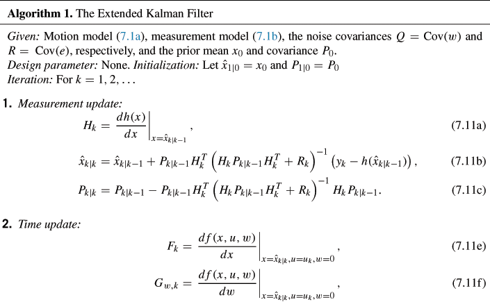
3.07.3.4 The extended Kalman filter
The Kalman filter recursions can be used for nonlinear filtering problems by applying a first order Taylor expansion of the model,

By re-arranging these equations, it can be seen as a linear model (7.10) with some additional terms in the right-hand side that do not depend on the state ![]() . Thus, the Kalman filter is easily modified for this approximate model. The resulting approximation of the Bayes optimal filter is called the extended Kalman filter.
. Thus, the Kalman filter is easily modified for this approximate model. The resulting approximation of the Bayes optimal filter is called the extended Kalman filter.
The extended Kalman filter consists of the following main steps:
![]() Define an initial Gaussian distribution
Define an initial Gaussian distribution ![]() for the state
for the state ![]() before the first observation
before the first observation ![]() is provided.
is provided.
1. Measurement update: use a Taylor approximation of (7.1b) and the analytical solution provided by the Kalman filter to get ![]() from
from ![]() .
.
2. Time update: use a Taylor approximation of (7.1a) and a simple formula from multivariate statistics to get ![]() from
from ![]() .
.
See Algorithm 1 for the details.
3.07.3.5 The unscented Kalman filter
The EKF takes care of the first two terms in a Taylor expansion of the model. The unscented Kalman filter (UKF) makes an attempt to also include the information in the quadratic term. Consider the following nonlinear mapping ![]() of a Gaussian vector x,
of a Gaussian vector x,
![]()

The unscented transform generates samples of ![]() , called sigma points, systematically on the surface of an ellipsoid centered around its mean, maps these points to
, called sigma points, systematically on the surface of an ellipsoid centered around its mean, maps these points to ![]() , and then computes the first two moments of the samples
, and then computes the first two moments of the samples ![]() . The procedure is quite similar to a Monte Carlo simulations, but there are two important differences: (1) the samples are deterministically chosen and (2) the weights in the mean and covariance estimators are not simply
. The procedure is quite similar to a Monte Carlo simulations, but there are two important differences: (1) the samples are deterministically chosen and (2) the weights in the mean and covariance estimators are not simply ![]() , where N is the number of samples.
, where N is the number of samples.
The following equations summarize the unscented transform. Let
![]() (7.12a)
(7.12a)
![]() (7.12b)
(7.12b)
where ![]() . Let
. Let ![]() , and apply
, and apply
 (7.13a)
 (7.13b)
![]() (7.13c)
(7.13c)
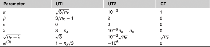
The design parameters of the UT are summarized below:
![]()
![]() controls the spread of the sigma points and is suggested to be approximately
controls the spread of the sigma points and is suggested to be approximately ![]() .
.
![]()
![]() compensates for the distribution, and should be chosen to
compensates for the distribution, and should be chosen to ![]() for Gaussian distributions.
for Gaussian distributions.
Note that ![]() when
when ![]() , and that for
, and that for ![]() the central weight
the central weight ![]() . Furthermore,
. Furthermore, ![]() . We will consider the two versions of UT in Table 7.1, corresponding to the original one in [15] and an improved one in [16]. Most interestingly, [17] describes a completely different approach yielding the same transformation with a different tuning. This approach starts from the integral defining the first two moments, and applies the cubature integration rule, hence the name cubature transform used here. It appears that this tuning gives a good result in many practically interesting cases, see Chapter 8 in [12] or [18].
. We will consider the two versions of UT in Table 7.1, corresponding to the original one in [15] and an improved one in [16]. Most interestingly, [17] describes a completely different approach yielding the same transformation with a different tuning. This approach starts from the integral defining the first two moments, and applies the cubature integration rule, hence the name cubature transform used here. It appears that this tuning gives a good result in many practically interesting cases, see Chapter 8 in [12] or [18].
As an illustration, the following mapping has a well-known distribution
![]() (7.14)
(7.14)
This distribution has mean n and variance ![]() . For the Taylor expansion, we get
. For the Taylor expansion, we get ![]() . This is of course not a useful approximation, but it is still what an EKF uses implicitly for quadratic functions. Now, the unscented transform gives
. This is of course not a useful approximation, but it is still what an EKF uses implicitly for quadratic functions. Now, the unscented transform gives ![]() and
and ![]() , respectively, for the three tunings in Table 7.1 (UT1, UT2, CT). This leads to useful approximations in filtering, except for the original UT1 for
, respectively, for the three tunings in Table 7.1 (UT1, UT2, CT). This leads to useful approximations in filtering, except for the original UT1 for ![]() (when the variance becomes negative).
(when the variance becomes negative).
Having defined the UT, the UKF can now be summarized as follows.
The unscented Kalman filter consists of the following main steps:
![]() Define an initial Gaussian distribution
Define an initial Gaussian distribution ![]() for the state
for the state ![]() before the first observation
before the first observation ![]() is provided.
is provided.
1. Measurement update: apply the unscented transform to (7.1b) and use an analytical result to get ![]() from
from ![]() .
.
2. Time update: apply the unscented transform to (7.1a) to immediately get ![]() from
from ![]() .
.
See Algorithm 2 for the details.
3.07.3.6 The particle filter
The particle filter (PF) works with a set of random trajectories. Each trajectory is formed recursively by iteratively simulating the model with some randomness, and then updating the likelihood of each trajectory based on the observed fingerprint:
The (marginalized) particle filter, (M)PF, for geolocation consists of the following main steps:
![]() Define a set of random positions (hypotheses, particles).
Define a set of random positions (hypotheses, particles).
![]() For each particle, define a random velocity vector.
For each particle, define a random velocity vector.
1. Compute the likelihood of the measurement fingerprint using the map.
2. Modify the weight (probability) of each particle.
3. Resample the set of particles.
4. Predict next position of the particles.
5. Marginalization step: update the velocity mean and covariance by a conditional Kalman filter.
See Algorithm 3 for the details.

3.07.3.6.1 Particle filter illustration
Figure 7.4 illustrates how the dynamic fingerprint depicted in Figure 7.1 is fitted to a road-map recursively in time. Initially, the particles are spread uniformly over a part of the road network corresponding to prior knowledge. The initial particle cloud can be seen in Figure 7.4b. Figure 7.4 shows how the particle cloud improves after each turn, to eventually become one single cloud, where a marker indicates that the position can be unambiguously estimated and used as input to the navigation system.
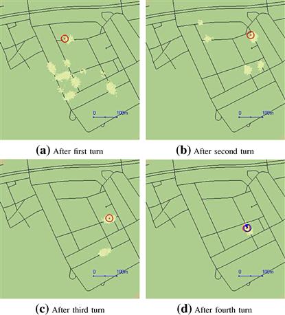
Figure 7.4 Illustration of how the particle representation of the position posterior distribution (course state is now shown) improves as the fingerprint becomes more informative. After four turns, the fingerprint is unique (unimodal posterior distribution), and a marker for geolocation is shown. The circle denotes GPS position, which is only used for evaluation purposes. Compare with Figure 7.1.
3.07.3.6.2 Particle filter details
Nonlinear filtering is the branch of statistical signal processing concerned with recursively estimating the state ![]() in (7.1) based on the measurements up to time
in (7.1) based on the measurements up to time ![]() from sample 1 to k. The most general problem it solves is to compute the Bayesian conditional posterior density
from sample 1 to k. The most general problem it solves is to compute the Bayesian conditional posterior density ![]() . The posterior distribution is in the particle filter approximated with
. The posterior distribution is in the particle filter approximated with
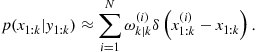 (7.16)
This is a weighted sum of Dirac distributions. A Dirac distribution is characterized with the identity ![]() for all smooth functions
for all smooth functions ![]() . This implies for instance that the mean of the trajectory is approximated with
. This implies for instance that the mean of the trajectory is approximated with
 (7.17)
Here ![]() denotes the likelihood of trajectory
denotes the likelihood of trajectory ![]() , given the observations
, given the observations ![]() . The likelihood of the dynamic fingerprint can be expressed as a conditional probability density function
. The likelihood of the dynamic fingerprint can be expressed as a conditional probability density function ![]() . Given a set of trajectories
. Given a set of trajectories ![]() with prior probabilities
with prior probabilities ![]() , the posterior probabilities become
, the posterior probabilities become
![]() (7.18)
(7.18)
This is the main principle for how the fingerprint is used to objectively compare the set of state trajectories. The particle filter does this in a recursive manner. Its simplest form is given in Algorithm 3.
Algorithm 3 gives the basic bootstrap or SIR particle filter, that works well when the sensor observations are not very accurate (of course, a relative notion). For more accurate observations, other so called proposal distributions should be used for the prediction step, and the weight update is modified accordingly, see [19] for the details. The last marginalization step will be illustrated in Section 3.07.4, when concrete motion models are given.
3.07.4 Motion models
The motion model ![]() in (7.1b) provides a description of how the object moves from time
in (7.1b) provides a description of how the object moves from time ![]() to time
to time ![]() when the next measurement is available. One interpretation is that the motion model describes how to interpolate between the position estimates computed from the measurements. It also relates position to other state variables, such as course and speed, and makes it possible to estimate these as well. The different classes of motion models are summarized below:
when the next measurement is available. One interpretation is that the motion model describes how to interpolate between the position estimates computed from the measurements. It also relates position to other state variables, such as course and speed, and makes it possible to estimate these as well. The different classes of motion models are summarized below:

We here describe a couple of specific and simple two-dimensional motion models that are typical for geolocation applications. Three-dimensional extensions do exist, but are much more complex, so we prefer to focus on horizontal position in two dimensions. See [20] or Chapters 12 and 13 in [12] for a survey on motion models.
3.07.4.1 Dead-reckoning model
A very instructive and also quite useful motion model is based on a state vector consisting of position ![]() and course (yaw angle)
and course (yaw angle) ![]() . This assumes that there are measurements of yaw rate (derivative of course)
. This assumes that there are measurements of yaw rate (derivative of course) ![]() and speed
and speed ![]() , in which case the principle of dead-reckoning can be applied. In ecology, dead-reckoning is more commonly called path integration.
, in which case the principle of dead-reckoning can be applied. In ecology, dead-reckoning is more commonly called path integration.
The dead-reckoning model can be formulated in continuous time using the following equations:
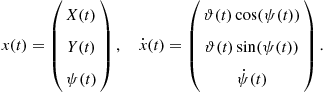 (7.20)
A discrete time model expressed at the sampling instants kT for the nonlinear dynamics is given by
 (7.21a)
 (7.21b)
![]() (7.21c)
(7.21c)
If the yaw rate ![]() is small compared to the sample interval T, then the model can be simplified. Further, assume that the speed
is small compared to the sample interval T, then the model can be simplified. Further, assume that the speed ![]() and angular velocity
and angular velocity ![]() are measured with some error
are measured with some error ![]() , with variance
, with variance ![]() and
and ![]() , respectively. This gives the following dynamic model with process noise
, respectively. This gives the following dynamic model with process noise ![]() :
:
![]() (7.22a)
(7.22a)
![]() (7.22b)
(7.22b)
![]() (7.22c)
(7.22c)
This model has the following structure:
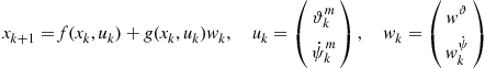 (7.22d)
that fits the particle filter perfectly. Note that the speed and the angular velocity measurements are modeled as inputs, rather than measurements. This is in accordance to many navigation systems, where inertial measurements are dead-reckoned in similar ways. The main advantage is that the state dimension is kept as small as possible, which is important for the particle filter performance and efficiency. This basic model can be used in a few different cases described next.
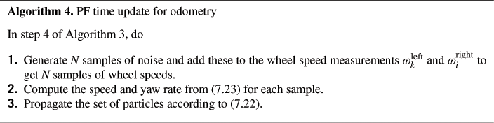
3.07.4.1.1 Odometric models
The wheel speeds ![]() and
and ![]() of two wheels with radius r on one axle of length L can be transformed to speed and yaw rate,
of two wheels with radius r on one axle of length L can be transformed to speed and yaw rate,
![]() (7.23a)
(7.23a)
![]() (7.23b)
(7.23b)
This fits the dead-reckoning model, and this special case is commonly referred to as odometry. The state vector might needs to be augmented with parameters for deviations from nominal wheel radius. For the road navigation example, the time update in Algorithm 3 can be given explicitly as in Algorithm 4
3.07.4.1.2 Inertial models
A course gyro provides ![]() and a longitudinal accelerometer give the acceleration
and a longitudinal accelerometer give the acceleration ![]() . If the state vector is extended with speed
. If the state vector is extended with speed ![]() to
to ![]() , and the state space model (7.22a–c) is extended with
, and the state space model (7.22a–c) is extended with ![]() , then we are back in the structure of (7.22d).
, then we are back in the structure of (7.22d).
3.07.4.1.3 Dynamical models
The steering and accelerator inputs to a car, or the rudder and engine commands to a vessel, can be statically mapped to speed ![]() and yaw rate
and yaw rate ![]() , and the dead-reckoning model can be applied directly. However, here the dynamics can be included to improve the motion model.
, and the dead-reckoning model can be applied directly. However, here the dynamics can be included to improve the motion model.
3.07.4.1.4 Marginalization of speed
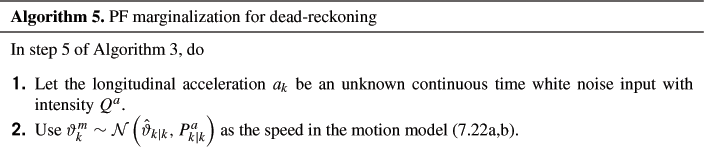
In inertial navigation, the state consists of four elements. Also in odometry and dynamical models, the speed is often used as a state. This fourth state usually increases the number of required particles in the PF substantially, and marginalization is recommended. The marginalization step 4 in Algorithm 3 can be used to eliminate the state ![]() from the PF. The marginalized particle filter is in general quite complex to implement [21], but for special cases like this the formulas become quite concrete, as shown in Algorithm 5.
from the PF. The marginalized particle filter is in general quite complex to implement [21], but for special cases like this the formulas become quite concrete, as shown in Algorithm 5.

We have only discussed two-dimensional models here, but the principles are easily extended to three dimensions. The state vector then includes the height ![]() , the roll
, the roll ![]() and the pitch
and the pitch ![]() angles. Thus, the state vector becomes about twice as large. In most practical application, the height is either trivial (surface vessels, cars) or an almost separate estimation problem (underwater vessels, aircraft), where pressure sensors provide accurate information to estimate height.
angles. Thus, the state vector becomes about twice as large. In most practical application, the height is either trivial (surface vessels, cars) or an almost separate estimation problem (underwater vessels, aircraft), where pressure sensors provide accurate information to estimate height.
3.07.4.2 Kinematic model
The simplest possible motion model, yet one of the most common ones in target tracking applications where no inertial measurements are available, is given by a two-dimensional version of Newton’s force law:
 (7.25a)
The corresponding discrete time model is given by
 (7.25b)
The time update in Algorithm 3 is here explicitly formulized in Algorithm 6.

3.07.4.2.1 Marginalization of speed
Suppose the sensor model depends on the position only, which is typical in geolocation applications,
![]() (7.26)
(7.26)
Since the motion model is linear in the state and noise, the marginalized PF applies, so the velocity component can be handled in a numerically very efficient way.
Let ![]() and
and ![]() . Then, (7.25b) and (7.26) can be rewritten as
. Then, (7.25b) and (7.26) can be rewritten as
![]() (7.27a)
(7.27a)
![]() (7.27b)
(7.27b)
![]() (7.27c)
(7.27c)
![]() (7.27d)
(7.27d)
We here use the particle filter for (7.27a,b) and the Kalman filter for (7.27c,d). Note that (7.27a) and (7.27d) are the same, but interpreted in two different ways. The time update in the particle filter becomes
![]() (7.28a)
(7.28a)
![]() (7.28b)
(7.28b)
![]() (7.28c)
(7.28c)
where we treat the velocity as a noise term. Conversely, we use the position as a measurement in the Kalman filter. For this particular structure, the general result given in Theorem 2.1 in [21] simplifies a lot, and we get a combined update
![]() (7.28d)
(7.28d)
 (7.28e)
Note that each particle has an individual velocity estimate ![]() but a common covariance
but a common covariance ![]() . Furthermore, if
. Furthermore, if ![]() , the covariance matrix converges quite quickly to zero,
, the covariance matrix converges quite quickly to zero, ![]() , and the Kalman filter is in fact not needed for the particle filter. The prediction step (7.28a,b) in the PF consists only of sampling from
, and the Kalman filter is in fact not needed for the particle filter. The prediction step (7.28a,b) in the PF consists only of sampling from ![]() in (7.28a). The Kalman and particle filters are thus decoupled.
in (7.28a). The Kalman and particle filters are thus decoupled.
3.07.5 Maps and applications
This part describes a number of applications in more detail. A summary of the applications and their features is provided in Table 7.2. The common theme of these applications is that they have been applied to real data and real maps, all using the (marginalized) particle filter. A detailed mathematical description of the particle filter and marginalized particle filter for some of these applications is provided in [19].
Table 7.2
Overview of the Illustrative Applications. The (marginalized) Particle Filter is Used in All of Them

To give some objective performance measure of the particle filter, the root mean square error (RMSE) of position (loosely speaking the standard deviation of the position error in meters) from the particle filter is in most cases below compared to a lower bound provided by the Cramer-Rao theory for nonlinear filters [14,22]. The lower bound is an information bound, that depends on the assumption in the model. Only asymptotically in information, the lower bound can be obtained. Since the same models are used in both the filter and bound, it can be used to judge the performance of the estimation method, here the particle filter. The particle filter performance can in theory never beat the lower bound. However, in practice it can, the typical case being when the actual measurements are more accurate than what is assumed in the model.
3.07.5.1 Road-bound vehicles
This application illustrates how the odometric model (7.22) with the wheel speed transformed measurements (7.23) is combined with a road map. First, the road map is discussed.
Figure 7.5 illustrates how a standard map can be converted to a likelihood function for the position. Positions on roads get the highest likelihood, and the likelihood quickly decays as the distance to the closest road increases. A small offset can be added to the likelihood function to allow for off-road driving, for instance on un-mapped roads and parking areas.

Figure 7.5 (a) Original map. (b) The road color is masked out, and local maxima over a ![]() region is computed to remove text information. (c) The resulting map is low-pass filtered to allow for small deviations from the road boarders, which yields a smooth likelihood function for on-road vehicles.
region is computed to remove text information. (c) The resulting map is low-pass filtered to allow for small deviations from the road boarders, which yields a smooth likelihood function for on-road vehicles.
The weights in the particle filter in Algorithm 3 are multiplied with the likelihood function in the measurement update (7.19a) as
![]() (7.29)
(7.29)
where one example of the likelihood function ![]() is shown graphically in Figure 7.5.
is shown graphically in Figure 7.5.
The likelihood function ![]() in (7.29), shown graphically in Figure 7.5c, is here used as a fingerprint. This summarizes the whole algorithm. This algorithm together with a complete navigation system including voice guidance was implemented in a student project on the platform shown in Figure 7.6 in 2001 [23]. Here, 15,000 particles were used in 2 Hz filter speed in this real-time GPS-free car navigation system. The conclusion from this project is that the computational complexity of the particle filter should not be overemphasized in practice.
in (7.29), shown graphically in Figure 7.5c, is here used as a fingerprint. This summarizes the whole algorithm. This algorithm together with a complete navigation system including voice guidance was implemented in a student project on the platform shown in Figure 7.6 in 2001 [23]. Here, 15,000 particles were used in 2 Hz filter speed in this real-time GPS-free car navigation system. The conclusion from this project is that the computational complexity of the particle filter should not be overemphasized in practice.

3.07.5.2 Airborne fast vehicles
Figure 7.7 illustrates the main concepts of terrain navigation [24,25]. The flying platform can compute the terrain altitude variations, and this dynamic fingerprint is matched to a terrain elevation map,
![]() (7.30)
(7.30)

Figure 7.7 (a) Framework of geolocation of airborne vehicles. The principle is that the down-looking radar provides distance to ground, while the barometer connected to the INS gives a reliable altitude estimate. The difference gives the altitude on ground. (b) The measured ground altitude is compared to a terrain elevation map, where the noise distribution models possible errors due to the radar lobe width and reflectors such as tree tops.
A separate vegetation classification map can be used to change the measurement noise distribution ![]() , where the idea is that the measurement from the radar is more reliable over an open field compared to a forest, for instance. In [24], it was shown that a Gaussian mixture is a good model for the radar altitude measurement error.
, where the idea is that the measurement from the radar is more reliable over an open field compared to a forest, for instance. In [24], it was shown that a Gaussian mixture is a good model for the radar altitude measurement error.
Figure 7.8a shows a flight trajectory overlayed on the topographic map. Figure 7.8b shows how the particle filter approximates the position distribution after the first few measurements. It is quite clear that the distribution is peaky with a lot of local maxima corresponding to positions with a good fit to the fingerprint. This is the strength of the particle filter compared to the classical Kalman filter, that can only handle one peak, or filterbanks, where the number of peaks must be specified beforehand.
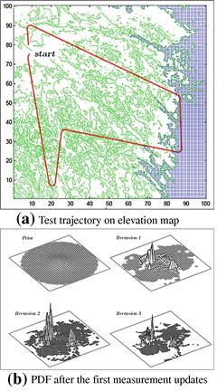
Figure 7.8 Flight trajectory overlayed the terrain elevation map (a). The position distribution after the first few iterations of the particle filter (b). Figures from [24].
Figure 7.9a shows the RMSE performance over time for the trajectory in Figure 7.8. The typical error is 10 m. One can notice that the RMSE grows when the aircraft is over the sea, since there is no information in the measurements.
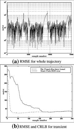
Figure 7.9 (a) RMSE as a function of sample number for the whole trajectory. (b) Zoom for the first initial phase. The RMSE is in both plots compared to the Cramer-Rao lower bound. Figures from [24].
Figure 7.9b shows the convergence of the particle filter, compared to the Cramer-Rao lower bound. Interestingly, the performance reaches the bound after 160 samples.
Finally, Figure 7.10 illustrates the information in the terrain elevation map. Figure 7.10a shows the map itself, and Figure 7.10b the RMSE bound as a function of position. One can here clearly identify the most informative areas at the highland, and the least informative over sea and lakes.

Figure 7.10 (a) Terrain elevation map. (b) Information content in the map, expressed as an expected value of the Cramer-Rao lower bound for each position. Figures from [24].
3.07.5.3 Airborne slow vehicles
The principle in the previous section assumes that the flying platform moves quickly compared to the terrain variations. For slow platforms such as unmanned aerial vehicles (UAV’s), this principle does not work. We here summarize another approach based on camera images of the ground.
Figure 7.11a shows the framework of the airborne geolocation system. A down-looking camera provides an aerial image that can in principle be compared to aerial photos in a database. However, this does not work in practice, due to large variations in light conditions and shadows, and also the seasonal variations. There is also a problem with a large dimensional search space. Even if the altitude of the platform is known, and the platform is assumed to be horizontal, there are still three degrees of freedom (two-dimensional translation and rotation). The solution described in [26] is based on the following steps:
![]() Make a circular cut of the image.
Make a circular cut of the image.
![]() Segment the image and classify each segment.
Segment the image and classify each segment.
![]() Use a histogram of the different segments as the fingerprint.
Use a histogram of the different segments as the fingerprint.
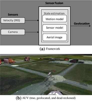
Figure 7.11 (a) Framework of geolocation of airborne vehicles. (b) Virtual reality snapshot of the AUV experiment.
Figure 7.12 summarizes some of the main steps in the particle filter. Due to the circular area of interest, the method is rotation invariant. A database of fingerprints for each position can easily be pre-computed from aerial photos. The resulting matching process is in this way computationally very attractive.

3.07.5.4 Underwater vessels
Figure 7.13 illustrates the framework for underwater navigation [27]. A sonar measures the distance to the seafloor. The control inputs (propeller speed and rudder angle) can be simulated in a dynamic model between the sampling instants in the prediction step in the particle filter. Alternatively, an inertial measurement unit can be used for the prediction step, possibly in combination with a Doppler velocity log.
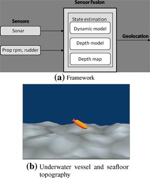
Figure 7.13 (a) Framework of geolocation of underwater vessels. (b) The principle is that a down-looking sonar provides distance to seafloor, while a pressure sensor (or up-looking sonar) gives the depth of the vessel. The difference gives the depth of the seafloor, which can be compared to a terrain elevation map.
Figure 7.14 shows an underwater map as described in [28]. Figure 7.14a shows the systematic trajectory used for mapping the seafloor using a surface vessel with sonar and GPS, together with a benchmark trajectory for evaluation purposes. Figure 7.14b shows the resulting seafloor map, with the ground truth trajectory, and the one obtained by just using the dynamical model (a simulation).
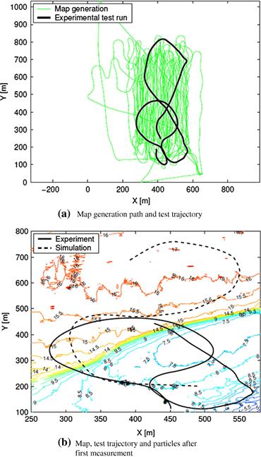
Figure 7.14 A surface vessel with GPS was used to map the area of interest in advance according to the systematic trajectory in (a), which also shows the test trajectory. The test trajectory is shown on the final map in (b).
Figure 7.15 shows the RMSE in the two position coordinates, compared to the Cramer-Rao lower bound. The performance is within a few meter error, and actually better than the bound, indicating that the measurements are more accurate than what is modeled.
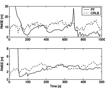
Figure 7.15 RMSE for the X and Y coordinates, respectively, for the whole trajectory in Figure 7.14.
3.07.5.5 Surface vessels
Figure 7.16a shows the framework for surface navigation using radar map matching principle [27]. Figure 7.16b shows a zoom of the sea chart in the upper left corner. The detections from a scanning radar are shown in polar coordinates in the top right corner. This is a fingerprint, which can be fitted in the area of the sea chart corresponding to our prior knowledge of position. This is a three-dimensional search (two position coordinates and one rotation). The particle filter solves this optimization for each radar scan, using a motion model to predict the motion and rotation of the radar platform.

Figure 7.16 (a) Framework of geolocation of surface vessels. (b) The principle is that the scanning radar provides a 360° view of the distance to shore, which can be compared to sea chart.
The performance of the filter is shown for one test trajectory in Figure 7.17a. The precision is most of the time in the order of 5 m, which is often more accurate than the coastline in a sea chart. Thus, this geolocation is even more useful for navigation than GPS, and in contrast to GPS it is not possible to jam. Between 50 and 60 s, the ship is moving out closer to open sea, thus decreasing the information in the radar scan. The performance is here somewhat worse than the lower bound.
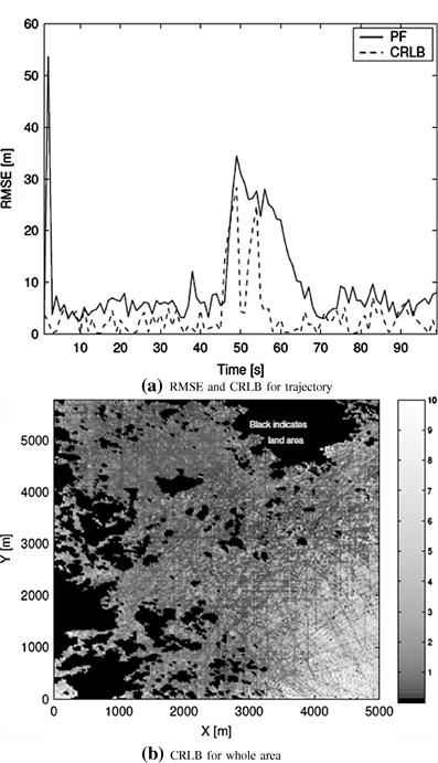
Figure 7.17 (a) RMSE for test trajectory as a function of time, in comparison to the CRLB. (b) The CRLB as a function of position, averaged over a set of straight line trajectories ending up at this spot. Figures from [27].
Figure 7.17b shows the lower bound on RMSE as a function of position. In this case, a number of random straight line trajectories are used to average the bound.
3.07.5.6 Cellular phones
Figure 7.18 shows the framework of geolocation based on received signal strength (RSS) and the transmitter’s identification number (ID). In this section, we survey results from a Wimax deployment in Brussels [29,30], but the same principle applies to all other cellular radio systems. At each time, a vector with n observed RSS values is obtained. The map provides a vector of m RSS values at each position (some grid is assumed here). A first problem is that n and m do not necessarily have to be the same, and the n ID’s do not even need to be a subset of the m ID’s in the map. One common solution is to only consider the largest set of common RSS elements. The advantage is that we can use the usual vector norms in the comparison of the measured fingerprint with the map. The disadvantage is that a missing ID gives a kind of negative information that is lost. That is, we can exclude areas based on a missing value from a certain site. A theoretically justified approach is still missing.

Figure 7.18 Framework of geolocation of cellular phones (a). The RSS map covers the highlighted road network from three sites (b) (from [29]).
3.07.5.6.1 Continuous RSS measurements
Figure 7.19 shows the RSS maps from three sites over the test area [29]. There are certain combinations of knowledge in the geolocation algorithm:
![]() One can use the static fingerprint and estimate the position independently at each time, or use a motion model and the particle filter to fit a dynamic fingerprint. We call these approaches static and dynamic, respectively.
One can use the static fingerprint and estimate the position independently at each time, or use a motion model and the particle filter to fit a dynamic fingerprint. We call these approaches static and dynamic, respectively.
![]() One can assume an arbitrary position, or that the position is constrained to the road network. We label this off-road or on-road, respectively.
One can assume an arbitrary position, or that the position is constrained to the road network. We label this off-road or on-road, respectively.
![]() The RSS vector from the map can either be an average computed from field tests, or based on generic path loss models, such as the Okamura-Hata model. The latter gives a quite course fingerprint map compared to the first one. We call these approaches OH and fingerprinting, respectively.
The RSS vector from the map can either be an average computed from field tests, or based on generic path loss models, such as the Okamura-Hata model. The latter gives a quite course fingerprint map compared to the first one. We call these approaches OH and fingerprinting, respectively.
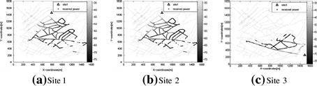
Figure 7.19 RSS fingerprint consists of the submaps from the available sites in the map. Figures from [29].
This gives in principle eight combinations, of which six ones are compared in Figure 7.20. The solid line is the same. The plots show the position error cumulative distribution function (CDF), rather than the averaged RMSE plots used otherwise. The reason is that the US FCC legislations for geolocation as required in the emergency response system. The rules are specified for the two marked levels (horizontal lines). For mobile-centric solutions, the error should be less than 50 m in 67% of all cases and less than 150 m in 95% of all cases.

Figure 7.20 RSS fingerprint consists of the submaps from the available sites in the map. Figures from [29].
Figure 7.20a shows that filtering improves the tail compared to snapshot estimation in the case of OH model for RSS. That is, filtering avoids heavy tails in the position error. The on-road constraint contributes significantly to the performance. With filtering, the FCC requirements are satisfied.
Figure 7.20b compares four different particle filters. It is here concluded that either the road constraint or the RSS fingerprint map should be used to get a significant improvement over a solution based on the OH model and arbitrary position. In that case, the FCC requirements are satisfied with margin.
3.07.5.6.2 Binary RSS measurements
A drawback with the continuous RSS map in the previous section is memory requirement. RSS is stored as integers in [0,127] for a dense grid on the road network. An alternative described in [30], is to store a binary value in larger grid areas. Figure 7.21 shows a binary dynamic fingerprint for a test drive.
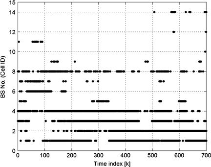
Figure 7.21 Example of dynamic fingerprint for binary RSS measurements. Figure from [30].
Figure 7.22a illustrates one grid area in the map. Each site serves two or three cells. The arrows shows the probability to get an RSS measurement from each cell averaged over the whole grid area. Figure 7.22b shows the cumulative density function when the algorithm is evaluated on a number of tests.
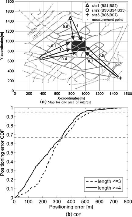
Figure 7.22 (a) Illustration of binary RSS map averaged over an area. (b) Result of binary fingerprinting. Compare with the measurement sequence in Figure 7.21. Figures from [30].
3.07.5.7 Small migrating animals
Figure 7.23 shows how the sunset or sunrise at each time defines a manifold on earth [4]. A sensor consisting of a light-logger and clock can detect these two events. This principle is applied in animal geolocation [31] using lightweight sensor units (0.5 g). The theory of geolocation by light levels is described in [6] for elephant seals, where sensitivity and geometrical relations are discussed in detail. The accuracy of the geolocation is evaluated on different sharks by comparing to a satellite navigation system, and the error is shown to be in the order of 1° in longitude and latitude. The first filter approach to this problem is presented in [32], where a particle filter is applied.
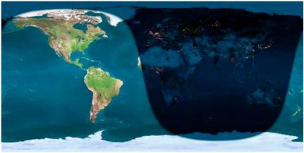
Figure 7.23 Binary day-light model for a particular time t. The shape of the dark area depends on the time of the year, and the horizontal position of the dark area depends on the time of the day. Source: Wikipedia.
The measurement model in the form of (7.1b) for the two events of sunset and sunrise, respectively, is
![]() (7.31a)
(7.31a)
![]() (7.31b)
(7.31b)
In this case, the measurement update (7.19a) in Algorithm 3 is
![]() (7.32)
(7.32)
![]()
Here, ![]() and
and ![]() denote the probability density functions for the light events.
denote the probability density functions for the light events.
If the animal is known to be at rest during the night, the two positions ![]() can be assumed the same, and the two unknowns can be solved from the two measurements uniquely, except for the two days of equinox when the sun is in the same plane as the equator, and thus the two manifolds in Figure 7.23 are vertical lines. Still, the PF gives useful information though the uncertainty in latitude increases, see Figure 7.24.
can be assumed the same, and the two unknowns can be solved from the two measurements uniquely, except for the two days of equinox when the sun is in the same plane as the equator, and thus the two manifolds in Figure 7.23 are vertical lines. Still, the PF gives useful information though the uncertainty in latitude increases, see Figure 7.24.
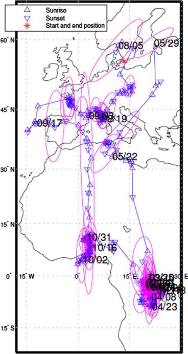
Figure 7.24 Estimated path of a Swift from 298 sunsets and sunrises, respectively. The ellipsoids illustrate a confidence interval at selected days. Figure from [32].
3.07.6 Mapping in practice
Many of the maps described here are publically or commerically available. Highly accurate topographic maps on dense grids are now available from satellite radar or laser measurements. Road maps and sea charts over whole continents are also available, though still with some absolute errors. This error will likely be corrected in the future based on aerial imagery and satellite measurements.
Maps of seafloor and magnetic field variations are still quite sparsely gridded, and not useful for geolocation. In particular the magnetic field, is time-varying, so regular updates of the map are required.
Cellular network maps of RSS or base station locations are also rapidly changing. Changes in the environment also affect the RSS values, which is particular true in indoor scenarios.
Thus, there is a need for efficient mapping algorithms that avoid manual tests to the largest possible extent. There are two main principles:
![]() Creating and adapting the map at the same time as performing geolocation. This approach is known as simultaneous localization and mapping (SLAM) in literature [33,34].
Creating and adapting the map at the same time as performing geolocation. This approach is known as simultaneous localization and mapping (SLAM) in literature [33,34].
Google Maps is an interesting project that illustrates two different principles for localization when GPS is not available. If a known WLAN is detected, whose ID is found in a database, the geolocation is based on the coverage of WLAN. The database is created by the company during street view campaigns. Second, if no WLAN is detected, the strongest RSS from the cellular network is used. Again, the ID is looked up in a map. This time, the map is created by users with GPS available. The map contains for each ID a circle covering a large fraction of the GPS reports.
The SLAM approach is best illustrated with an example, here taken from [35]. The surface navigation application based on radar scan matching to a sea chart in Section 3.07.5.5 is revisited, assuming that there is no sea chart available. This might not be a relevant example in practice, but the idea is easily extended to seafloor mapping, earth magnetic field mapping, indoor RSS mapping, etc.
Figure 7.25 shows the test trajectory (upper left), the boat (lower left) and the radar scans overlayed on eachother to form a sea chart like map (right). Here, also the estimated first half of the test trajectory is plotted. No other information than the radar scans has been used, which shows that clever algorithms can actually solve the complex mapping task autonomously.

Figure 7.25 Simultaneous geolocation of surface ships and generation of a sea chart. Figures from [35].
3.07.7 Conclusion
Geolocation is the art of innovative combination of properties of nature and sensor technology. We have provided a set of applications illustrating how different sensors and maps (geographical information systems) can be used to compute geolocation. The particle filter has been used as a general method for geolocation. Fingerprinting is a general concept for fitting measurements (along a trajectory) to a map.
Relevant Theory: Statistical Signal Processing and Machine Learning
See Vol. 1, Chapter 19 A Tutorial Introduction to Monte Carlo Methods, Markov Chain Monte Carlo and Particle Filtering
See this Volume, Chapter 1 Introduction to Statistical Signal Processing
See this Volume, Chapter 4 Bayesian Computational Methods in Signal Processing
References
1. Altizer S, Bartel R, Han BA. Animal migration and infectious disease risk. Science. 2011;331:296–302.
2. Muir JA, Van oorschot PC. Internet geolocation: evasion and counterevasion. ACM Comput Surv (CSUR). 2009;42.
3. Katz-Bassett E, John JP, Krishnamurthy A, Wetherall D, Anderson T, Chawathe Y. Towards IP geolocation using delay and topology measurements. In: Proceedings of the Sixth ACM SIGCOMM Conference on Internet, Measurement. 2006.
4. Meeus JH. Astronomical Algorithms. Willmann-Bell, Inc. 1991.
5. Tyren C. Magnetic terrain navigation. In: Fifth International Symposium on Unmanned Untethered Submersible Technology. 1987.
6. Hill Roger D. Theory of geolocation by light levels. In: Le Boeuf Burney J, Laws Richard M, eds. Elephant Seals: Population Ecology, Behavior, and Physiology. University of California Press 1994.
7. Teo SLH, Boustany A, Blackwell S, Walli A, Weng KC, Block BA. Validation of geolocation estimates based on light level and sea surface temperature from electronic tags. Mar Ecol Prog Ser. 2004;283:81–88.
8. Gustafsson F, Gunnarsson F. Mobile positioning using wireless networks: possibilities and fundamental limitations based on available wireless network measurements. IEEE Signal Process Mag. 2005;22:41–53.
9. Hui L, Darabi H, Banerjee P, Jing L. Survey of wireless indoor positioning techniques and systems. IEEE Trans Syst Man Cybern Part C Appl Rev. 2007;37(6):1067–1080.
10. Pahlavan K, Xinrong L, Makela JP. Indoor geolocation science and technology. IEEE Commun Mag. 2002;40(2):112–118.
11. Rantakokko Jouni, Rydell Joakim, Stromback Peter, et al. Accurate and reliable soldier and first responder indoor positioning: multisensor systems and cooperative localization. IEEE Wirel Commun. 2011;18(2):10–18.
12. F. Gustafsson, Statistical Sensor Fusion, Studentlitteratur, second ed., 2010.
13. Bergman N. Recursive Bayesian Estimation: Navigation and Tracking Applications. Sweden: Linköping University; 1999; Dissertation no. 579.
14. Tichavsky P, Muravchik CH, Nehorai A. Posterior Cramér-Rao bounds for discrete-time nonlinear filtering. IEEE Trans Signal Process. 1998;46(5):1386–1396.
15. Julier SJ, Uhlmann JK, Durrant-Whyte Hugh F. A new approach for filtering nonlinear systems. In: IEEE American Control Conference. 1995;1628–1632.
16. E.A. Wan, R. van der Merwe, The unscented Kalman filter for nonlinear estimation, in: Proceedings of IEEE Symposium (AS-SPCC), pp. 153–158.
17. Arasaratnam I, Haykin S, Elliot RJ. Cubature Kalman filter. IEEE Trans Autom Control. 2009;54:1254–1269.
18. Gustafsson Fredrik, Hendeby Gustaf. Some relations between extended and unscented Kalman filters. IEEE Trans Signal Process. 2012;60(2):545–555 funding agencies—Swedish research council (VR).
19. Gustafsson F. Particle filter theory and practice with positioning applications. IEEE Trans Aerosp Electron Mag. 2010;7:53–82.
20. Li XR, Jilkov VP. Survey of maneuvering target tracking Part I: dynamic models. IEEE Trans Aerosp Electron Syst. 2003;39(4):1333–1364.
21. Schön TB, Gustafsson F, Nordlund PJ. Marginalized particle filters for nonlinear state-space models. IEEE Trans Signal Process. 2005;53:2279–2289.
22. Bergman N. Posterior Cramér-Rao bounds for sequential estimation. In: Doucet A, de Freitas N, Gordon N, eds. Sequential Monte Carlo Methods in Practice. Springer-Verlag 2001.
23. Forssell U, Hall P, Ahlqvist S, Gustafsson F. Novel map-aided positioning system. In: Proceedings of FISITA, No F02-1131, Helsinki. 2002.
24. Bergman N, Ljung L, Gustafsson F. Terrain navigation using Bayesian statistics. IEEE Control Syst Mag. 1999;19(3):33–40.
25. Nordlund P-J, Gustafsson F. Marginalized particle filter for accurate and reliable terrain-aided navigation. IEEE Trans Aerosp Electron Syst. 2009.
26. Skoglar P, Orguner U, Törnqvist D, Gustafsson F. In: IEEE Aerospace Conference. 2010.
27. Karlsson R, Gustafsson F. Bayesian surface and underwater navigation. IEEE Trans Signal Process. 2006;54(11):4204–4213.
28. T. Karlsson, Terrain aided underwater navigation using Bayesian statistics, Master Thesis LiTH-ISY-EX-3292, Dept. Elec. Eng., Linköping University, S-581 83 Linköping, Sweden, 2002.
29. M. Bshara, U. Orguner, F. Gustafsson, L. Van Biesen, Fingerprinting localization in wireless networks based on received signal strength measurements: a case study on wimax networks, 2010. <http://www.control.isy.liu.se/fredrik/reports/09tvtmussa.pdf>.
30. Bshara M, Orguner U, Gustafsson F, VanBiesen L. Robust tracking in cellular networks using HMM filters and cell-ID measurements. 2011;60(3):1016–1024.
31. Alerstam T, Hedenström A, A˚kesson S. Long-distance migration: evolution and determinants. Oikos. 2003;103(2):247–260.
32. Wahlström Niklas, Gustafsson Fredrik, A˚kesson Susanne. A voyage to Africa by Mr Swift. In: Proceedings of 15th International Conference on Information Fusion, Singapore. July 2012.
33. Bailey T, Durrant-Whyte H. Simultaneous localization and mapping (SLAM): Part II. IEEE Robot Autom Mag. 2006;13(3):108–117.
34. Durrant-Whyte H, Bailey T. Simultaneous localization and mapping (SLAM): Part I. IEEE Robot Autom Mag. 2006;13(2):99–110.
35. Callmer J, Törnqvist D, Svensson H, Carlbom P, Gustafsson F. Radar SLAM using visual features. EURASIP J Adv Signal Process. 2011.