
Performance Analysis and Bounds
Brian M. Sadler and Terrence J. Moore, Army Research Laboratory, Adelphi, MD, USA
Abstract
This chapter is an overview of performance analysis in statistical signal processing, including analysis of estimators, and related performance bounds. We survey key ideas and related tools for the analysis of algorithms, including parametric and non-parametric estimators. We also consider the Cramer-Rao bound in detail, including constraints. Bounds provide fundamental limits on estimation given some assumptions on the probability laws and a model for the parameters of interest. Together, fundamental bounds and analysis of algorithms go hand in hand to provide a complete picture.
Keywords
Estimation; Maximum likelihood; Parametric model; Non-parametric model; Additive noise; Multiplicative noise; Gaussian noise; Non-Gaussian noise; Cramer-Rao bound; Constrained Cramer-Rao bound; Central limit theorem; Mean square error; Bias; Perturbation theory; Least squares estimation; Monte Carlo methods; Confidence intervals
3.08.1 Introduction
In this chapter we consider performance analysis of estimators, as well as bounds on estimation performance. We introduce key ideas and avenues for analysis, referring to the literature for detailed examples. We seek to provide a description of the analytical procedure, as well as to provide some insight, intuition, and guidelines on applicability and results.
Bounds provide fundamental limits on estimation given some assumptions on the probability laws and a model for the parameters of interest. Bounds are intended to be independent of the particular choice of estimator, although any nontrivial bound requires some assumptions, e.g., a bound may hold for some class of estimators, or may be applicable only for unbiased estimators, and so on.
On the other hand, given a specific estimation algorithm, we would like to analytically characterize its performance as a function of the relevant system parameters, such as available data length, signal-to-noise ratio (SNR), etc. Together, fundamental bounds and analysis of algorithms go hand in hand to provide a complete picture.
We begin with the specific, examining the classic theory of parameterized probability models, and the associated Cramér-Rao bounds and their relationship with maximum likelihood estimation. These ideas are fundamental to statistical signal processing, and understanding them provides a significant foundation for general understanding. We then consider mean square error analysis more generally, as well as perturbation methods for algorithm small-error analysis that is especially useful for algorithms that rely on subspace decompositions. We also describe the more recent theory of the constrained Cramér-Rao bound, and its relationship with constrained maximum-likelihood estimation.
We examine the case of a parameterized signal with both additive and multiplicative noise in detail, including Gaussian and non-Gaussian cases. The multiplicative random process introduces signal variations as commonly arise with propagation through a randomly fluctuating medium. General forms for the CRB for estimating signal parameters in multiplicative and additive noise are available that encompass many cases of interest.
We next consider asymptotic analysis, as facilitated by the law of large numbers and the central limit theorem. In particular, we consider two fundamental and broadly applied cases, the asymptotics of Fourier coefficients, and asymptotics of nonlinear least squares estimators. Under general conditions, both result in tractable expressions for the estimator distribution as it converges to a Gaussian.
Finally, we look at Monte Carlo methods for evaluating expressions involving random variables, such as numerical evaluation of the Cramér-Rao bound when obtaining an analytical expression is challenging. We close with a discussion of confidence intervals that provide statistical evidence of estimator quality, often based on asymptotic arguments, and can be computed from the given data.
3.08.2 Parametric statistical models
Let ![]() denote an N-dimensional probability density function (pdf) that depends on the parameters in the vector
denote an N-dimensional probability density function (pdf) that depends on the parameters in the vector ![]() . The vector
. The vector ![]() is a collection of random variables. For example, suppose
is a collection of random variables. For example, suppose ![]() describes a normal distribution with independent and identically distributed (iid) elements each with variance
describes a normal distribution with independent and identically distributed (iid) elements each with variance ![]() . Then the parameters describing the pdf are
. Then the parameters describing the pdf are ![]() , where
, where ![]() is the mean vector. With the iid assumption, the covariance is completely determined by the scalar variance
is the mean vector. With the iid assumption, the covariance is completely determined by the scalar variance ![]() ; see Section 3.08.2.1.4. Here,
; see Section 3.08.2.1.4. Here, ![]() are random variables from a normal distribution with the specified mean and variance. In the 1-D case, such as a scalar time series
are random variables from a normal distribution with the specified mean and variance. In the 1-D case, such as a scalar time series ![]() , the random variables may be stacked into the vector
, the random variables may be stacked into the vector ![]() , and
, and ![]() is the joint pdf of N consecutive observations of
is the joint pdf of N consecutive observations of ![]() .
.
When we have samples from the random process then we can think of the vector ![]() as containing a realization of the random process governed by the pdf; now the contents of
as containing a realization of the random process governed by the pdf; now the contents of ![]() are also often called the observations. This can be confusing because we have not altered the notation, but have altered our interpretation of
are also often called the observations. This can be confusing because we have not altered the notation, but have altered our interpretation of ![]() to be a function of
to be a function of ![]() , with a given set of observations
, with a given set of observations ![]() regarded as fixed and known constants. In this interpretation, the pdf is called the likelihood function.
regarded as fixed and known constants. In this interpretation, the pdf is called the likelihood function.
The functional description ![]() is remarkably general, incorporating knowledge of the underlying model via the functional dependence on the parameters in
is remarkably general, incorporating knowledge of the underlying model via the functional dependence on the parameters in ![]() , and expressing randomness (i.e., lack of specific knowledge about
, and expressing randomness (i.e., lack of specific knowledge about ![]() ) through the distribution. Much of the art of statistical signal processing is defining the model for a specific problem, expressed in
) through the distribution. Much of the art of statistical signal processing is defining the model for a specific problem, expressed in ![]() , that can sufficiently capture the essential nature of the observations, lead to tractable and useful signal processing algorithms, and enable performance analysis. We seek the smallest dimensionality in
, that can sufficiently capture the essential nature of the observations, lead to tractable and useful signal processing algorithms, and enable performance analysis. We seek the smallest dimensionality in ![]() such that the underlying model remains sufficiently detailed to capture the behavior of the observations, while not over-parameterizing in a way that adds too much complexity or unneeded model variation. It is important to keep in mind that a model is a useful abstraction. Over-specifying the model may be as bad as underspecification. While a large number of parameters may be appealing to better fit some observed data, the model can easily lose generality and become too cumbersome to manipulate and estimate its parameters. On the other hand, if the model is underspecified then it may be too abstract to capture essential behavior. All of this motivates exploration of families of models and levels of abstraction. A key component of performance analysis in this context is to explore the pros and cons of models in their descriptive power.
such that the underlying model remains sufficiently detailed to capture the behavior of the observations, while not over-parameterizing in a way that adds too much complexity or unneeded model variation. It is important to keep in mind that a model is a useful abstraction. Over-specifying the model may be as bad as underspecification. While a large number of parameters may be appealing to better fit some observed data, the model can easily lose generality and become too cumbersome to manipulate and estimate its parameters. On the other hand, if the model is underspecified then it may be too abstract to capture essential behavior. All of this motivates exploration of families of models and levels of abstraction. A key component of performance analysis in this context is to explore the pros and cons of models in their descriptive power.
In statistical signal processing we are often interested in a signal plus noise model. Expressed in 1-D, we have
![]() (8.1)
(8.1)
where ![]() is a deterministic parameterized signal model, and
is a deterministic parameterized signal model, and ![]() is an additive random process modeling noise and/or interference. The most basic assumptions typically begin with assuming
is an additive random process modeling noise and/or interference. The most basic assumptions typically begin with assuming ![]() are samples from a stationary independent Gaussian process, i.e., additive white Gaussian noise (AWGN). AWGN is fundamental for several reasons; it models additive thermal noise arising in sensors and their associated electronics, it arises through the combination of many small effects as described through the central limit theorem, it is often the worst case as compared with additive iid non-Gaussian noise (see Section 3.08.7), and Gaussian processes are tractable and fully specified by their first and second-order statistics. (We can generalize (8.1) so that the signal
are samples from a stationary independent Gaussian process, i.e., additive white Gaussian noise (AWGN). AWGN is fundamental for several reasons; it models additive thermal noise arising in sensors and their associated electronics, it arises through the combination of many small effects as described through the central limit theorem, it is often the worst case as compared with additive iid non-Gaussian noise (see Section 3.08.7), and Gaussian processes are tractable and fully specified by their first and second-order statistics. (We can generalize (8.1) so that the signal ![]() is also a random process, in which case it is also common to assume the noise is statistically independent of the signal.) Note that for
is also a random process, in which case it is also common to assume the noise is statistically independent of the signal.) Note that for ![]() , then information about
, then information about ![]() in the observations
in the observations ![]() is contained in the time-varying mean
is contained in the time-varying mean ![]() . If instead
. If instead ![]() is a function of the parameters in
is a function of the parameters in ![]() , then there is information about
, then there is information about ![]() in the covariance of
in the covariance of ![]() . A fundamental extension to (8.1) incorporates propagation of
. A fundamental extension to (8.1) incorporates propagation of ![]() through a linear channel, given by
through a linear channel, given by ![]() where
where ![]() denotes convolution. The observation model (8.1) is the tip of the iceberg for a vast array of models that incorporate aspects such as man-made signals or naturally occurring signals, interference, and the physics of sensors and electronics. Understanding of performance analysis for (8.1) is fundamental to these many cases.
denotes convolution. The observation model (8.1) is the tip of the iceberg for a vast array of models that incorporate aspects such as man-made signals or naturally occurring signals, interference, and the physics of sensors and electronics. Understanding of performance analysis for (8.1) is fundamental to these many cases.
Given observations ![]() , let
, let
![]() (8.2)
(8.2)
be an estimator of ![]() . Performance analysis primarily focuses on two objectives. First, we wish to find bounds on the possible performance of
. Performance analysis primarily focuses on two objectives. First, we wish to find bounds on the possible performance of ![]() , without specifying
, without specifying ![]() . To do this we typically need some further assumptions or restrictions on the possible form or behavior of
. To do this we typically need some further assumptions or restrictions on the possible form or behavior of ![]() . For example, we might consider only those estimators that are unbiased so that
. For example, we might consider only those estimators that are unbiased so that ![]() . Or, we might restrict our attention to the class of
. Or, we might restrict our attention to the class of ![]() that are linear functions of the observations, so
that are linear functions of the observations, so ![]() for some matrix H. The second objective is to analyze the performance of a specific estimator. We are given a specific estimation algorithm
for some matrix H. The second objective is to analyze the performance of a specific estimator. We are given a specific estimation algorithm ![]() and we wish to assess its performance. These two objectives are bound together, and their combination provides a clear picture; comparing algorithm performance with bounds will reveal the optimality or sub-optimality of the algorithm, and helps guide the development of good algorithms.
and we wish to assess its performance. These two objectives are bound together, and their combination provides a clear picture; comparing algorithm performance with bounds will reveal the optimality or sub-optimality of the algorithm, and helps guide the development of good algorithms.
The most commonly applied algorithm and performance framework for parametric models is maximum likelihood estimation (MLE) and the Cramér-Rao bound (CRB). These are directly related, as described in the following.
In the context of performance analysis, it can be useful to evaluate the MLE and compare it to the CRB, even if the MLE has undesirably high complexity. This gives us a benchmark to compare other algorithms against. For example, we might simplify our assumptions, or derive an approximation to the MLE, resulting in an algorithm with lower complexity. We can then explore the complexity-performance tradeoff in a meaningful way.
3.08.2.1 Cramér-Rao bound on parameter estimation
The Cramér-Rao bound (CRB) is the most widely applied technique for bounding our ability to estimate ![]() given observations from
given observations from ![]() . The basic definition is as follows. Suppose we have an observation
. The basic definition is as follows. Suppose we have an observation ![]() in
in ![]() from the pdf
from the pdf ![]() where
where ![]() is a vector of deterministic parameters in an open set
is a vector of deterministic parameters in an open set ![]() . The Fisher information matrix (FIM) for this model is given by
. The Fisher information matrix (FIM) for this model is given by
![]() (8.3)
(8.3)
where ![]() is the Fisher score defined by
is the Fisher score defined by
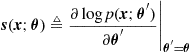 (8.4)
(8.4)
and the expectation is evaluated at ![]() , i.e.,
, i.e., ![]() . We assume certain regularity conditions, namely that the pdf is differentiable with respect to
. We assume certain regularity conditions, namely that the pdf is differentiable with respect to ![]() and satisfies
and satisfies
![]() (8.5)
(8.5)
for both ![]() and
and ![]() where
where ![]() is an unbiased estimator of
is an unbiased estimator of ![]() [1]. Intuitively, existence of the bound relies on the smoothness of the pdf in the parameters, and that the allowable range of the parameters does not have hard boundaries where the derivatives may fail to exist. Regularity and the assumption that
[1]. Intuitively, existence of the bound relies on the smoothness of the pdf in the parameters, and that the allowable range of the parameters does not have hard boundaries where the derivatives may fail to exist. Regularity and the assumption that ![]() is in an open set guarantee this.
is in an open set guarantee this.
Evaluation of ![]() in (8.3) uses the product of first derivatives of
in (8.3) uses the product of first derivatives of ![]() . Note the condition in (8.5) when
. Note the condition in (8.5) when ![]() permits us to substitute
permits us to substitute
![]() (8.6)
(8.6)
in (8.3), yielding
 (8.7)
(8.7)
Equation (8.7) provides an alternative expression for the FIM in terms of second-order derivatives of ![]() , that in some cases may be easier to evaluate.
, that in some cases may be easier to evaluate.
The regularity condition in (8.5) is assured when the Jacobian and Hessian of the density function ![]() are absolutely integrable with respect to both
are absolutely integrable with respect to both ![]() and
and ![]() [2], and this essentially permits switching the order of integration and differentiation. This is the most commonly assumed regularity condition, although other scenarios can ensure regularity is satisfied. Under these assumptions, we have the following Cramér-Rao bound theorem (sometimes referred to as the information inequality) [1–4], that was independently developed by Cramér [5] and Rao [6].
[2], and this essentially permits switching the order of integration and differentiation. This is the most commonly assumed regularity condition, although other scenarios can ensure regularity is satisfied. Under these assumptions, we have the following Cramér-Rao bound theorem (sometimes referred to as the information inequality) [1–4], that was independently developed by Cramér [5] and Rao [6].
Given appropriate regularity conditions on ![]() as above, the variance of any unbiased estimator
as above, the variance of any unbiased estimator ![]() of
of ![]() satisfies the inequality
satisfies the inequality
![]() (8.8)
(8.8)
if the inverse exists, and the variance is exactly ![]() if and only if
if and only if
![]() (8.9)
(8.9)
(in the mean-square sense). We refer to the inverse of the Fisher information matrix as the Cramér-Rao bound and denote it as
![]() (8.10)
(8.10)
where the CRB on the ith element of ![]() is given by the ith element of the diagonal of
is given by the ith element of the diagonal of ![]() .
.
3.08.2.1.1 CRB on transformations of the parameters
The performance of estimation of a function of the parameters, e.g., the transformation ![]() , is often of more interest than the performance of direct estimation of the parameters. Note that
, is often of more interest than the performance of direct estimation of the parameters. Note that ![]() and
and ![]() need not have the same dimension. If the Jacobian of the transformation function is
need not have the same dimension. If the Jacobian of the transformation function is ![]() , then the CRB on the performance of an unbiased estimator
, then the CRB on the performance of an unbiased estimator ![]() of
of ![]() is given in the following [1,4]. The variance of any unbiased estimator
is given in the following [1,4]. The variance of any unbiased estimator ![]() of
of ![]() satisfies the inequality
satisfies the inequality
![]() (8.11)
(8.11)
with equality if and only if ![]() (in the mean-square sense). Equation (8.11) relates the CRB on
(in the mean-square sense). Equation (8.11) relates the CRB on ![]() to the CRB on
to the CRB on ![]() by incorporating the Jacobian of the function
by incorporating the Jacobian of the function ![]() that transforms
that transforms ![]() to
to ![]() . Implicit in (8.11) is that
. Implicit in (8.11) is that ![]() is differentiable with respect to
is differentiable with respect to ![]() and (8.5) must also be satisfied for
and (8.5) must also be satisfied for ![]() .
.
3.08.2.1.2 The bias-informed CRB
The CRB theory above applies only to unbiased estimates. But suppose we have a particular biased estimator of ![]() , given by
, given by ![]() , with bias given by
, with bias given by ![]() . We can use (8.11) to find a bound on
. We can use (8.11) to find a bound on ![]() . Because
. Because ![]() is an unbiased estimator of the function
is an unbiased estimator of the function ![]() , it follows that
, it follows that
![]() (8.12)
(8.12)
where
![]() (8.13)
(8.13)
with ![]() . We refer to (8.12) as the bias-informed CRB.
. We refer to (8.12) as the bias-informed CRB.
The bias-informed CRB only applies to the class of estimators with the specified bias gradient ![]() , and does not provide a general bound for an arbitrary biased estimator. Because of this the bias-informed CRB has limited use and has not found broad application. An approach that seeks to overcome this to some extent is the uniform CRB, that broadens the applicability of the bias-informed CRB to the class of estimators whose bias function is nearly constant over a region [7,8]. When a closed form is not available the bias-gradient can be computed numerically, at least for problems that have relatively few parameters [7].
, and does not provide a general bound for an arbitrary biased estimator. Because of this the bias-informed CRB has limited use and has not found broad application. An approach that seeks to overcome this to some extent is the uniform CRB, that broadens the applicability of the bias-informed CRB to the class of estimators whose bias function is nearly constant over a region [7,8]. When a closed form is not available the bias-gradient can be computed numerically, at least for problems that have relatively few parameters [7].
3.08.2.1.3 A general CRB expression
The above results on parameter transformation and estimator bias are special cases of a combined general CRB expression, given by
![]() (8.14)
(8.14)
where ![]() is an estimator of
is an estimator of ![]() with bias
with bias ![]() ,
, ![]() is the CRB matrix for estimating
is the CRB matrix for estimating ![]() , and
, and
![]() (8.15)
(8.15)
is the sum of the Jacobian of the parameter transformation and the bias gradient. The previous expressions then follow as special cases. For example, the CRB on estimation of ![]() for unbiased estimators is given by (8.11) with
for unbiased estimators is given by (8.11) with ![]() since
since ![]() . Or, the CRB on estimation of
. Or, the CRB on estimation of ![]() with a biased estimator
with a biased estimator ![]() whose bias is
whose bias is ![]() , is given by (8.12) with
, is given by (8.12) with ![]() since there is no parameter transformation (i.e.,
since there is no parameter transformation (i.e., ![]() is the identity transformation). When introducing the CRB, some texts begin with (8.10), whereas others begin with (8.14) or one of the variations.
is the identity transformation). When introducing the CRB, some texts begin with (8.10), whereas others begin with (8.14) or one of the variations.
3.08.2.1.4 Normal distributions
When the density function ![]() is Gausian, denoted
is Gausian, denoted ![]() , then the Cramér-Rao bound is completely characterized by the dependence on the parameter
, then the Cramér-Rao bound is completely characterized by the dependence on the parameter ![]() of the mean
of the mean ![]() and covariance
and covariance ![]() . Assuming differentiability with respect to
. Assuming differentiability with respect to ![]() , then the CRB can be evaluated in terms of otherwise arbitrary functions for the mean
, then the CRB can be evaluated in terms of otherwise arbitrary functions for the mean ![]() and covariance
and covariance ![]() , and the CRB is given by the Slepian-Bangs formula [9,10],
, and the CRB is given by the Slepian-Bangs formula [9,10],
 (8.16)
There are many examples of application of (8.16), e.g., see Kay [4]. When the signal plus Gaussian noise model of (8.1) holds, then covariance ![]() is not a function of
is not a function of ![]() , and the second term in (8.16) vanishes.
, and the second term in (8.16) vanishes.
3.08.2.1.5 Properties of the CRB
We discuss some properties and interpretation of the CRB.
![]() CRB existence and regularity conditions: An example where the CRB does not exist due to violation of the regularity conditions occurs when estimating the parameters of a uniform distribution. Specifically, suppose we have observations
CRB existence and regularity conditions: An example where the CRB does not exist due to violation of the regularity conditions occurs when estimating the parameters of a uniform distribution. Specifically, suppose we have observations ![]() from a uniform distribution on
from a uniform distribution on ![]() , and we seek the CRB on estimation of
, and we seek the CRB on estimation of ![]() . Now, the regularity conditions do not hold and the CRB cannot be applied. This is a classic text book example, see Kay [4, Problem 3.1].
. Now, the regularity conditions do not hold and the CRB cannot be applied. This is a classic text book example, see Kay [4, Problem 3.1].
![]() The CRB is a local bound: As we know from basic calculus, the second derivative corresponds to the curvature or concavity of the function at a point on the curve. Thus the CRB, evaluated at a particular value of the parameter
The CRB is a local bound: As we know from basic calculus, the second derivative corresponds to the curvature or concavity of the function at a point on the curve. Thus the CRB, evaluated at a particular value of the parameter ![]() , can be interpreted as the expected value of the curvature of the likelihood around the parameter. This is an important interpretation since the curvature measure is local, and consequently the CRB is often referred to as a local bound. We remark on this point again when considering the asymptotic behavior of the MLE in the next section. Because it is a local bound the CRB at a parameter value
, can be interpreted as the expected value of the curvature of the likelihood around the parameter. This is an important interpretation since the curvature measure is local, and consequently the CRB is often referred to as a local bound. We remark on this point again when considering the asymptotic behavior of the MLE in the next section. Because it is a local bound the CRB at a parameter value ![]() gives us a tight lower bound on the variance of any unbiased estimator of
gives us a tight lower bound on the variance of any unbiased estimator of ![]() only when the estimation errors are small. Depending on the particular scenario, this might correspond to obtaining a large number of observations, or a high signal-to-noise ratio (SNR). This also means that the CRB can be a loose lower bound for the opposite cases, when the number of observations is low, or at low SNR.
only when the estimation errors are small. Depending on the particular scenario, this might correspond to obtaining a large number of observations, or a high signal-to-noise ratio (SNR). This also means that the CRB can be a loose lower bound for the opposite cases, when the number of observations is low, or at low SNR.
![]() Effect of adding parameters: If an additional parameter is brought into the model, so that the dimension of
Effect of adding parameters: If an additional parameter is brought into the model, so that the dimension of ![]() grows by one, then the bound on the previously existing parameters will remain the same or rise. It will remain the same if the new parameter is decoupled from the previous parameters in the model. Or, if the parameters are coupled, the bound can only increase. Intuitively, this is because the introduction of a new unknown into the model can only increase uncertainty, implying more difficulty in obtaining accurate parameter estimates, and hence a larger bound. The proof relies on linear algebra and is a standard textbook problem, e.g., see Kay [4, Problem 3.11].
grows by one, then the bound on the previously existing parameters will remain the same or rise. It will remain the same if the new parameter is decoupled from the previous parameters in the model. Or, if the parameters are coupled, the bound can only increase. Intuitively, this is because the introduction of a new unknown into the model can only increase uncertainty, implying more difficulty in obtaining accurate parameter estimates, and hence a larger bound. The proof relies on linear algebra and is a standard textbook problem, e.g., see Kay [4, Problem 3.11].
![]() Not necessarily a tight bound: Generally there is no guarantee that an estimator exists that can achieve the CRB. More typically, under certain conditions the MLE can be shown to asymptotically achieve the CRB, but there is no guarantee this will occur with finite data; see the discussion below on the MLE in Section 3.08.3. Other bounds exist that may be tighter than the CRB in the non-asymptotic region, such as bounding the mean square error; see Section 3.08.4.
Not necessarily a tight bound: Generally there is no guarantee that an estimator exists that can achieve the CRB. More typically, under certain conditions the MLE can be shown to asymptotically achieve the CRB, but there is no guarantee this will occur with finite data; see the discussion below on the MLE in Section 3.08.3. Other bounds exist that may be tighter than the CRB in the non-asymptotic region, such as bounding the mean square error; see Section 3.08.4.
![]() Identifiability: Given the parametric model, we would like the distribution function to be distinguishable by the choice of the parameters. In other words, we want a given pdf
Identifiability: Given the parametric model, we would like the distribution function to be distinguishable by the choice of the parameters. In other words, we want a given pdf ![]() to be unique on some non-zero measurable set for different choices of
to be unique on some non-zero measurable set for different choices of ![]() . If not, e.g., supposing
. If not, e.g., supposing ![]() yet
yet ![]() for almost every
for almost every ![]() , then we cannot uniquely infer anything about the parameters even with an infinite number of observations. This is the problem of identifiability. While there are various definitions and contexts for identifiability, here we can note that a fundamental requirement for the existence of the CRB is that the Fisher information matrix be full rank so that it’s inverse exists. Generally nonsingularity in the FIM evaluated at the true value of the parameter implies identifiability locally about the parameter [11], reflecting the fact that the CRB is a local bound governed by the local smooth behavior of the pdf. For example, for the Gaussian pdf case, Hochwald and Nehorai showed there exists a strong link between identifiability and nonsingularity in the FIM [12].
, then we cannot uniquely infer anything about the parameters even with an infinite number of observations. This is the problem of identifiability. While there are various definitions and contexts for identifiability, here we can note that a fundamental requirement for the existence of the CRB is that the Fisher information matrix be full rank so that it’s inverse exists. Generally nonsingularity in the FIM evaluated at the true value of the parameter implies identifiability locally about the parameter [11], reflecting the fact that the CRB is a local bound governed by the local smooth behavior of the pdf. For example, for the Gaussian pdf case, Hochwald and Nehorai showed there exists a strong link between identifiability and nonsingularity in the FIM [12].
Consider scalar cases such as ![]() , or
, or ![]() , where
, where ![]() is additive Gaussian noise and we wish to find the CRB on estimation of a and b. For both examples we find that the FIM is not full rank, hence the CRB does not exist. Studying the models for the observation x, it is apparent that we cannot uniquely identify the parameter(s). This situation can be resolved if there is additional information in the form of equality constraints on the parameters; see Section 3.08.6.
is additive Gaussian noise and we wish to find the CRB on estimation of a and b. For both examples we find that the FIM is not full rank, hence the CRB does not exist. Studying the models for the observation x, it is apparent that we cannot uniquely identify the parameter(s). This situation can be resolved if there is additional information in the form of equality constraints on the parameters; see Section 3.08.6.
![]() Biased estimators: It can happen that the MLE is a biased estimator, even with infinite data. An interesting example is the estimation of the covariance of a multivariate normal distribution. Given
Biased estimators: It can happen that the MLE is a biased estimator, even with infinite data. An interesting example is the estimation of the covariance of a multivariate normal distribution. Given ![]() , the maximum likelihood estimator for
, the maximum likelihood estimator for ![]() is the sample covariance using observations of
is the sample covariance using observations of ![]() . However, it has been shown that this estimate is biased, and so the CRB does not bound the MLE in this case, e.g., see Chen et al. [13]. For more on biased estimators see Sections 3.08.2.1.2 and 3.08.4.
. However, it has been shown that this estimate is biased, and so the CRB does not bound the MLE in this case, e.g., see Chen et al. [13]. For more on biased estimators see Sections 3.08.2.1.2 and 3.08.4.
![]() Estimation versus classification bounds: The CRB bounds continuous estimation of a continuous parameter. In this case perfect (zero-error) estimation is not possible. Suppose instead the parameter is drawn from a finite set, e.g., we draw from a finite alphabet for communicating symbols. Now, the parameter is discrete valued, and perfect estimation is possible. In such a case the CRB goes to zero; it is uninformative. The problem is now one of classification, rather than estimation, and a classification bound is needed for performance analysis, such as bit error rate bounds in digital communications [14,15].
Estimation versus classification bounds: The CRB bounds continuous estimation of a continuous parameter. In this case perfect (zero-error) estimation is not possible. Suppose instead the parameter is drawn from a finite set, e.g., we draw from a finite alphabet for communicating symbols. Now, the parameter is discrete valued, and perfect estimation is possible. In such a case the CRB goes to zero; it is uninformative. The problem is now one of classification, rather than estimation, and a classification bound is needed for performance analysis, such as bit error rate bounds in digital communications [14,15].
3.08.3 Maximum likelihood estimation and the CRB
The CRB provides a lower bound on the variance of any unbiased estimator, subject to the regularity conditions on ![]() . Next we consider the maximum-likelihood estimator, which has the remarkable property that under some basic assumptions the estimate will asymptotically achieve the CRB, and therefore achieves asymptotic optimality.
. Next we consider the maximum-likelihood estimator, which has the remarkable property that under some basic assumptions the estimate will asymptotically achieve the CRB, and therefore achieves asymptotic optimality.
The maximum likelihood approach to estimation of ![]() chooses as an estimator
chooses as an estimator ![]() that, if true, would have the highest probability (the maximum likelihood) of resulting in the given observations
that, if true, would have the highest probability (the maximum likelihood) of resulting in the given observations ![]() . Thus, the MLE results from the optimization problem
. Thus, the MLE results from the optimization problem
![]() (8.17)
(8.17)
where for convenience ![]() may be equivalently maximized since
may be equivalently maximized since ![]() is a monotonic transformation. Previously we thought of
is a monotonic transformation. Previously we thought of ![]() as fixed constants in the pdf
as fixed constants in the pdf ![]() . Now, in (8.17), we are given observations
. Now, in (8.17), we are given observations ![]() and regard
and regard ![]() as a function of
as a function of ![]() . In this case
. In this case ![]() is referred to as the likelihood function.
is referred to as the likelihood function.
Using basic optimization principles, a solution of (8.17) follows by solving the equations resulting from differentiating with respect to the parameters and setting these equations equal to zero. The derivatives of the log-likelihood are the Fisher score previously defined in (8.4), so the first-order conditions for finding the MLE are solutions ![]() of
of
![]() (8.18)
(8.18)
Applying (8.18) requires smoothness in the parameters so that the derivatives exist. The parameters lie in a (possibly infinite) set, denoted ![]() . Then, assuming the derivatives exist and provided
. Then, assuming the derivatives exist and provided ![]() is an open set,
is an open set, ![]() will satisfy (8.18). Intuitively, the solution to (8.18) relies on the smoothness of the function in the parameters, and the parameters themselves do not have hard boundaries where the derivatives may fail to exist. This is similar to the assumptions needed for the existence of the CRB on
will satisfy (8.18). Intuitively, the solution to (8.18) relies on the smoothness of the function in the parameters, and the parameters themselves do not have hard boundaries where the derivatives may fail to exist. This is similar to the assumptions needed for the existence of the CRB on ![]() ; see the discussion in Section 3.08.2.1.
; see the discussion in Section 3.08.2.1.
The principle of maximum likelihood provides a systematic approach to estimation given the parametric model ![]() . If (8.18) cannot be solved in closed form, we can fall back on optimization algorithms applied directly to (8.17). Many sophisticated tools and algorithms have been developed for this over the past several decades. Very often the maximization is non-convex, although our smoothness conditions guarantee local convexity in some neighborhood around the true value for
. If (8.18) cannot be solved in closed form, we can fall back on optimization algorithms applied directly to (8.17). Many sophisticated tools and algorithms have been developed for this over the past several decades. Very often the maximization is non-convex, although our smoothness conditions guarantee local convexity in some neighborhood around the true value for ![]() , so algorithms often consist of finding a good initial value and then seeking the local maximum.
, so algorithms often consist of finding a good initial value and then seeking the local maximum.
If the parameters take on values from a discrete set then the assumptions on the solution of (8.18) are violated. However, the MLE may still exist although estimation will generally rely directly on (8.17). Note that in this case we have a classification rather than an estimation problem: choose ![]() from a discrete set of possible values that provides the maximum in (8.17). Consequently, the CRB is not applicable and performance analysis will rely on classification bounds; see the comment in Section 3.08.2.1.5.
from a discrete set of possible values that provides the maximum in (8.17). Consequently, the CRB is not applicable and performance analysis will rely on classification bounds; see the comment in Section 3.08.2.1.5.
3.08.3.1 Asymptotic normality and consistency of the MLE
As we noted, the MLE has a fundamental link with the CRB, as described next. Let the samples ![]() be iid observations from the pdf
be iid observations from the pdf ![]() . Denote
. Denote ![]() to be the collection of these samples. Then, the likelihood is given by
to be the collection of these samples. Then, the likelihood is given by ![]() , and we denote the maximum likelihood estimate from these samples as
, and we denote the maximum likelihood estimate from these samples as ![]() .
.
Assuming appropriate regularity conditions on the pdf ![]() hold, such as described above, then the MLE of the parameter
hold, such as described above, then the MLE of the parameter ![]() is asymptotically distributed according to
is asymptotically distributed according to
![]() (8.19)
(8.19)
where ![]() is derived from the pdf
is derived from the pdf ![]() , i.e., it is the Fisher information of a single observation or sample, and
, i.e., it is the Fisher information of a single observation or sample, and ![]() denotes convergence in distribution.
denotes convergence in distribution.
This remarkable property states that the MLE is asymptotically normally distributed as observation size n goes to infinity, is unbiased so that ![]() converges to
converges to ![]() in the mean, and has covariance given by the CRB. Thus, the MLE is asymptotically optimal because the CRB is a lower bound on the variance of any unbiased estimator. Intuitively, the asymptotic normal distribution of the estimate occurs due to a central limit theorem effect. Note that only general regularity conditions (e.g., smoothness) are required on
in the mean, and has covariance given by the CRB. Thus, the MLE is asymptotically optimal because the CRB is a lower bound on the variance of any unbiased estimator. Intuitively, the asymptotic normal distribution of the estimate occurs due to a central limit theorem effect. Note that only general regularity conditions (e.g., smoothness) are required on ![]() for this to (eventually) be true. We discuss the central limit theorem more generally in Section 3.08.8.
for this to (eventually) be true. We discuss the central limit theorem more generally in Section 3.08.8.
Equation (8.19) shows that the MLE is consistent. A consistent estimator is one that converges in probability to ![]() , meaning that the distribution of
, meaning that the distribution of ![]() becomes more tightly concentrated around
becomes more tightly concentrated around ![]() as n grows. In the specific case of the MLE, as n grows the distribution of the estimator converges to a Gaussian distribution with mean given by the true parameter and covariance given by the CRB, and this distribution is collapsing around the true value as we obtain more observations. If the mean of
as n grows. In the specific case of the MLE, as n grows the distribution of the estimator converges to a Gaussian distribution with mean given by the true parameter and covariance given by the CRB, and this distribution is collapsing around the true value as we obtain more observations. If the mean of ![]() were not equal to the true value of
were not equal to the true value of ![]() , then the estimator would be converging to the wrong answer. And, since the variance of the MLE converges to the CRB, we are assured that the MLE is asymptotically optimal, implying that as the data size becomes large no other estimator will have a distribution that collapses faster around the true value.
, then the estimator would be converging to the wrong answer. And, since the variance of the MLE converges to the CRB, we are assured that the MLE is asymptotically optimal, implying that as the data size becomes large no other estimator will have a distribution that collapses faster around the true value.
3.08.4 Mean-square error bound
As we have noted the CRB is only valid for unbiased estimators, whereas we may have an estimator that is biased. If the bias is known and we can compute its gradient then we can use the bias-informed CRB, but as we noted this is rarely the case. More generally we may be interested in analyzing the bias-variance tradeoff, for example with finite data an estimator may be biased even if it is asymptotically unbiased and approaches the CRB for large data size. This naturally leads to the mean-square error (MSE) of the estimator, given by
![]() (8.20)
(8.20)
The variance and the MSE of the estimator ![]() are easily related through
are easily related through
![]() (8.21)
(8.21)
and they are equivalent in the unbiased case, so that if ![]() is unbiased then the CRB bounds both the variance and the MSE. If the estimator remains biased even as the observation size grows, then the MSE may become dominated by the bias error asymptotically.
is unbiased then the CRB bounds both the variance and the MSE. If the estimator remains biased even as the observation size grows, then the MSE may become dominated by the bias error asymptotically.
Study of the MSE can be valuable when relatively fewer observations are available. In this regime an estimator may trade off bias and variance, with the goal of minimizing the MSE. It may be tempting to say that a particular biased estimator is “better” than the CRB when MSE![]() , but the CRB only bounds unbiased estimators; it is better to refer to Eqs. (8.20) or (8.21) that quantify the relationship. Ultimately, as the number of observations grows, then it is desired to have the estimate become unbiased and the variance of the estimator diminish, otherwise the estimator will asymptotically converge to the wrong answer.
, but the CRB only bounds unbiased estimators; it is better to refer to Eqs. (8.20) or (8.21) that quantify the relationship. Ultimately, as the number of observations grows, then it is desired to have the estimate become unbiased and the variance of the estimator diminish, otherwise the estimator will asymptotically converge to the wrong answer.
The MSE and bias-variance tradeoff is also valuable for choosing a particular model, e.g., see Spall [16, Chapter 12].
In Section 3.08.2.1.5, when discussing biased estimators, we noted that the MLE for the covariance of a multivariate normal distribution is just the sample covariance, and that in this case the MLE is a biased estimator. In addition, the sample covariance is not a minimum MSE estimator for this problem, in the sense of minimizing the expected Frobenius norm squared of the error matrix. In fact, a lower MSE can be obtained by the James-Stein estimator, that uses a shrinkage-regularization estimation technique [13,17]. This example illustrates that the maximum likelihood estimator is not necessarily guaranteed to achieve the minimum MSE among biased or unbiased estimators.
3.08.5 Perturbation methods for algorithm analysis
Perturbation methods provide an approach to small-error analysis of algorithms. This is a close relative of using a Taylor expansion and dropping higher order terms. Consequently, perturbation analysis is accurate for larger data size, and so can be thought of as an asymptotic analysis, and it will generally predict asymptotic performance. The idea has been broadly applied, especially for cases when the estimation algorithm is a highly nonlinear function of the data and/or the model parameters. An important application area occurs when algorithms incorporate matrix decompositions, such as subspace methods in array processing. However, we emphasize that the ideas are general and can be readily applied in many scenarios.
3.08.5.1 Perturbations and statistical analysis
The general idea is as follows. A statistical perturbation error analysis consists of two basic steps. The first is a deterministic step, adding small perturbations into the model at the desired place. The perturbations can be applied to the original data such as occurs with additive noise. But, the perturbations can also be applied at other stages, such as perturbing the estimate itself. The perturbed model is then manipulated to obtain an expression for the estimation error as a function of the perturbations, where (typically) only the first order perturbation terms are kept, and terms that involve higher order functions of the perturbation are dropped under the assumption that they are negligible. The second step is statistical. We now assume the perturbations are random variables drawn from a stationary process with finite variance (typically zero-mean), and proceed to evaluate the statistics of the estimation error expression. This typically involves the mean and variance of the first-order perturbed estimation error expression.
Let ![]() be an estimator of parameters
be an estimator of parameters ![]() , which we write as
, which we write as ![]() , where
, where ![]() is a small perturbation. Therefore, we have the simple estimation error expression
is a small perturbation. Therefore, we have the simple estimation error expression
![]() (8.22)
(8.22)
To quantify the error in the estimator, we wish to find quantities such as the mean and variance of the estimation error expression. Thus we treat ![]() as samples from a stationary random process, commonly assumed to be zero-mean independent and identically distributed; it is not necessary to specify the pdf of the perturbation. The important point is that when deriving (8.22) for the specific estimator of interest we make use of the small error assumption and keep only first-order terms in
as samples from a stationary random process, commonly assumed to be zero-mean independent and identically distributed; it is not necessary to specify the pdf of the perturbation. The important point is that when deriving (8.22) for the specific estimator of interest we make use of the small error assumption and keep only first-order terms in ![]() . Derivation of (8.22) is the primary hurdle to this analytical approach, so that we can evaluate
. Derivation of (8.22) is the primary hurdle to this analytical approach, so that we can evaluate ![]() and
and ![]() . If
. If ![]() then the algorithm is unbiased for small error (this may mean the algorithm is asymptotically unbiased).
then the algorithm is unbiased for small error (this may mean the algorithm is asymptotically unbiased).
The perturbation method is appealing when an algorithm is biased. If ![]() then we can use it with
then we can use it with ![]() to find the MSE in Eq. (8.21). This enables study of the bias-variance tradeoff, for cases where the CRB does not apply due to the estimator bias. For example, the perturbation method has been applied to geolocation based on biased range measurements, such that the estimation of the source location is inherently biased [18].
to find the MSE in Eq. (8.21). This enables study of the bias-variance tradeoff, for cases where the CRB does not apply due to the estimator bias. For example, the perturbation method has been applied to geolocation based on biased range measurements, such that the estimation of the source location is inherently biased [18].
While the accuracy of first order perturbation analysis is generally limited to the high SNR and/or large data regime, the perturbation method can be broadened by considering second-order terms, as developed by Xu for subspace methods [19]. The resulting error expressions now contain more terms, but the resulting analyses are more accurate over a larger range of SNR and data size (roughly speaking, the second-order analyses are accurate for moderate to large SNR or data size).
3.08.5.2 Matrix perturbations
As we noted an important application of these ideas is for algorithms that involve matrix decompositions. These algorithms are typically not very amenable to error analysis because the estimation error expression becomes highly nonlinear in the parameters of interest. Instead, we can apply a perturbation to the matrix and then study the effect of the perturbation after the matrix decomposition.
Suppose we have an ![]() matrix
matrix ![]() , that is input to an algorithm for estimating some parameters
, that is input to an algorithm for estimating some parameters ![]() . Often an algorithm includes an eigendecomposition of
. Often an algorithm includes an eigendecomposition of ![]() (for
(for ![]() ), or more generally with a singular value decomposition (SVD) of
), or more generally with a singular value decomposition (SVD) of ![]() (for
(for ![]() ). To carry out the first step in the perturbation based analysis, we would like to express the matrix decomposition as a function of a perturbation on
). To carry out the first step in the perturbation based analysis, we would like to express the matrix decomposition as a function of a perturbation on ![]() .
.
Let ![]() be a perturbed version of
be a perturbed version of ![]() , where
, where ![]() is small. Regarding
is small. Regarding ![]() as deterministic, Stewart developed expressions for many important cases, carrying the perturbations along. These include the eigenvalues of
as deterministic, Stewart developed expressions for many important cases, carrying the perturbations along. These include the eigenvalues of ![]() , the singular values of
, the singular values of ![]() , the subspaces of
, the subspaces of ![]() , as well as the pseudo-inverse of
, as well as the pseudo-inverse of ![]() , projections, and linear least squares algorithms [20–22]. These expressions generally rely on keeping only first-order terms in
, projections, and linear least squares algorithms [20–22]. These expressions generally rely on keeping only first-order terms in ![]() , and dropping higher-order terms under the assumption that
, and dropping higher-order terms under the assumption that ![]() is small, where here small is meant in the sense of some appropriate matrix norm [22].
is small, where here small is meant in the sense of some appropriate matrix norm [22].
If an estimation algorithm is a function of ![]() and involves subspace decomposition say, then we can use the expressions from Stewart in our approach. Given the perturbed subspace, we then find the estimation error expression, that is now a function of
and involves subspace decomposition say, then we can use the expressions from Stewart in our approach. Given the perturbed subspace, we then find the estimation error expression, that is now a function of ![]() , again keeping only the first order terms. The analysis is then completed by finding the statistical properties of the error, such as mean and variance.
, again keeping only the first order terms. The analysis is then completed by finding the statistical properties of the error, such as mean and variance.
Many array processing methods rely on subspace decomposition and eigenvalue expressions [23], and consequently the perturbation ideas have been broadly applied to develop small error analysis [24]. Perturbations can be applied to the data, or to the estimated spatial covariance matrix, for example [19]. These applications typically use complex values, and the perturbation ideas readily go over from the real-valued to the complex-valued case.
3.08.5.3 Obtaining the CRB through perturbation analysis of the MLE
An important special case is the application of perturbation analysis to the MLE. Now, under the conditions for which the MLE is consistent, i.e., is asymptotically unbiased and attains the CRB, then the perturbation approach can yield the CRB by finding the variance of the estimation error expression as above. This follows because we are carrying out a small error (asymptotic) analysis for an algorithm that is asymptotically guaranteed to achieve a variance that is equal to the CRB. For examples, see [18,25].
3.08.6 Constrained Cramér-Rao bound and constrained MLE
In this section we show how the classic parametric statistical modeling framework from Sections 3.08.2 and 3.08.3, including the CRB and MLE, can be extended by incorporating additional information in the form equality constraints. We make the same assumptions as in Section 3.08.2, given observations ![]() from a probability density function
from a probability density function ![]() where
where ![]() is a vector of unknown deterministic parameters. Suppose now that these parameters satisfy k consistent and nonredundant continuously differentiable parametric equality constraints. These constraints can be expressed as a vector function
is a vector of unknown deterministic parameters. Suppose now that these parameters satisfy k consistent and nonredundant continuously differentiable parametric equality constraints. These constraints can be expressed as a vector function ![]() for some
for some ![]() . Equivalently, the constraints can also be stated
. Equivalently, the constraints can also be stated ![]() , i.e., the equality constraints act to restrict the parameters to a subset of the original parameter space. The constraints being consistent means that the set
, i.e., the equality constraints act to restrict the parameters to a subset of the original parameter space. The constraints being consistent means that the set ![]() is nonempty, and the constraints being nonredundant means that the Jacobian
is nonempty, and the constraints being nonredundant means that the Jacobian ![]() has rank k whenever
has rank k whenever ![]() .
.
The presence of the constraints provides further specific additional information about the model ![]() , expressed functionally as
, expressed functionally as ![]() . Equivalently, in addition to obeying
. Equivalently, in addition to obeying ![]() the parameters are also restricted to live in
the parameters are also restricted to live in ![]() . Intuitively, we can expect that more accurate estimation should be possible, and that we can incorporate the constraints into both performance bounds and estimators. This is the case, and we detail the extension of the CRB and MLE to incorporate the constraints in the following.
. Intuitively, we can expect that more accurate estimation should be possible, and that we can incorporate the constraints into both performance bounds and estimators. This is the case, and we detail the extension of the CRB and MLE to incorporate the constraints in the following.
3.08.6.1 Constrained CRB
The following relates the Fisher information ![]() for the original unconstrained model
for the original unconstrained model ![]() , to a new bound on
, to a new bound on ![]() that incorporates the constraints [26, Theorem 1]. Let
that incorporates the constraints [26, Theorem 1]. Let ![]() be an unbiased estimator of
be an unbiased estimator of ![]() , where in addition equality constraints are imposed as above so that
, where in addition equality constraints are imposed as above so that ![]() , or equivalently
, or equivalently ![]() . Then
. Then
![]() (8.23)
(8.23)
where ![]() is a matrix whose column vectors form an orthonormal basis for the null space of the Jacobian
is a matrix whose column vectors form an orthonormal basis for the null space of the Jacobian ![]() , i.e.,
, i.e.,
![]() (8.24)
(8.24)
In (8.24), ![]() is an
is an ![]() identity matrix (not to be confused with the Fisher information matrix
identity matrix (not to be confused with the Fisher information matrix ![]() ). Equation (8.23) defines the constrained Cramér-Rao bound (CCRB) on
). Equation (8.23) defines the constrained Cramér-Rao bound (CCRB) on ![]() . Equality in the bound is achieved if and only if
. Equality in the bound is achieved if and only if ![]() (in the mean-square sense), where
(in the mean-square sense), where ![]() is the Fisher score defined in (8.4). This is similar to the condition for achieving equality with the CRB noted earlier.
is the Fisher score defined in (8.4). This is similar to the condition for achieving equality with the CRB noted earlier.
The CCRB can be extended to bound transformations of parameters, just as for the CRB in Section 3.08.2.1.1. Consider a continuously differentiable function of the parameters ![]() and denote its Jacobian as
and denote its Jacobian as ![]() . Given constraints
. Given constraints ![]() , then the variance of any unbiased estimator
, then the variance of any unbiased estimator ![]() of
of ![]() satisfies the inequality
satisfies the inequality
![]() (8.25)
(8.25)
This extends the CCRB on ![]() to the parameters
to the parameters ![]() , and has a form similar to (8.11).
, and has a form similar to (8.11).
3.08.6.2 Comments and properties of the CCRB
![]() Existence and regularity conditions: It is important to recognize that the CCRB relies on the Fisher information
Existence and regularity conditions: It is important to recognize that the CCRB relies on the Fisher information ![]() expressed through the probability density
expressed through the probability density ![]() . We have not altered the construction of the Fisher score or FIM in (8.4) and (8.3). The constraints are regarded as additional side information, resulting in the CCRB.
. We have not altered the construction of the Fisher score or FIM in (8.4) and (8.3). The constraints are regarded as additional side information, resulting in the CCRB.
Note that the CCRB does not require ![]() be nonsingular, but does require that
be nonsingular, but does require that ![]() be nonsingular. Thus the addition of constraints can lead to a meaningful bound on estimation even when the original model is not identifiable. For example, constraints can lead to bounds on blind estimation problems [26,27].
be nonsingular. Thus the addition of constraints can lead to a meaningful bound on estimation even when the original model is not identifiable. For example, constraints can lead to bounds on blind estimation problems [26,27].
![]() Constrained estimators versus constrained parameters: Stoica and Ng actually developed a bound for an unbiased, constrained estimator, as opposed to a bound for an unbiased estimator of constrained parameters [26]. This is an important distinction since, in general, a parameter and its unbiased estimator will not simultaneously satisfy a constraint. The conditions for when this does occur, i.e., when
Constrained estimators versus constrained parameters: Stoica and Ng actually developed a bound for an unbiased, constrained estimator, as opposed to a bound for an unbiased estimator of constrained parameters [26]. This is an important distinction since, in general, a parameter and its unbiased estimator will not simultaneously satisfy a constraint. The conditions for when this does occur, i.e., when ![]() , are the equality conditions for Jensen’s inequality. Many of the citations of Stoica and Ng mistakenly apply the bound to the case of constrained parameters. Fortunately, the result under either assumption is the same CCRB expression, even if the interpretation is different [28].
, are the equality conditions for Jensen’s inequality. Many of the citations of Stoica and Ng mistakenly apply the bound to the case of constrained parameters. Fortunately, the result under either assumption is the same CCRB expression, even if the interpretation is different [28].
![]() Reparameterizing the model: An equally valid approach to bounding estimation performance is to reparameterize the pdf in a way that incorporates the constraints, resulting in a distribution
Reparameterizing the model: An equally valid approach to bounding estimation performance is to reparameterize the pdf in a way that incorporates the constraints, resulting in a distribution ![]() with new parameter vector
with new parameter vector ![]() . Then the Fisher information
. Then the Fisher information ![]() can be obtained for the reparameterized model, and the CRB results in Section 3.08.2 can be applied to bound estimation of
can be obtained for the reparameterized model, and the CRB results in Section 3.08.2 can be applied to bound estimation of ![]() or functions of
or functions of ![]() . Obviously
. Obviously ![]() , and it often happens that the dimension of
, and it often happens that the dimension of ![]() is less than the dimension of
is less than the dimension of ![]() because the constraints amount to a manifold reduction by requiring
because the constraints amount to a manifold reduction by requiring ![]() [29]. However, reparameterizing the model into
[29]. However, reparameterizing the model into ![]() can often be analytically impractical or numerically complex. The CCRB offers an alternative way to incorporate parametric equality constraints into the CRB and, for example, enables comparison of a variety of constraints in a straightforward way.
can often be analytically impractical or numerically complex. The CCRB offers an alternative way to incorporate parametric equality constraints into the CRB and, for example, enables comparison of a variety of constraints in a straightforward way.
![]() Inequality constraints: The CCRB directly incorporates equality constraints. In some problems, the parameters are specified to obey inequality constraints. In such a case, the conventional CRB applies so long as the specified value of
Inequality constraints: The CCRB directly incorporates equality constraints. In some problems, the parameters are specified to obey inequality constraints. In such a case, the conventional CRB applies so long as the specified value of ![]() obeys the inequality, and so is a feasible value.
obeys the inequality, and so is a feasible value.
![]() Evaluating the CCRB: Evaluating the CCRB requires evaluating
Evaluating the CCRB: Evaluating the CCRB requires evaluating ![]() , which is typically straightforward analytically, and then finding the nullspace basis
, which is typically straightforward analytically, and then finding the nullspace basis ![]() (and note that
(and note that ![]() is not unique). The matrix
is not unique). The matrix ![]() may be found analytically, or it can be readily computed numerically, e.g., using standard software packages.
may be found analytically, or it can be readily computed numerically, e.g., using standard software packages.
3.08.6.3 Constrained MLE
Just as the CRB is intimately related with maximum-likelihood estimation, the CCRB is related with constrained maximum-likelihood estimation (CMLE). The CMLE ![]() solves the constrained optimization problem given by
solves the constrained optimization problem given by
 (8.26)
We can also show that given appropriate smoothness conditions, ![]() converges in distribution to
converges in distribution to ![]() . Thus, asymptotically, the CMLE becomes normally distributed with mean equal to the true parameter and covariance given by the CCRB. This is analogous to the classic results for the MLE in (8.19). For derivations and details, including CMLE cast as a constrained scoring algorithm, see Moore et al. [30].
. Thus, asymptotically, the CMLE becomes normally distributed with mean equal to the true parameter and covariance given by the CCRB. This is analogous to the classic results for the MLE in (8.19). For derivations and details, including CMLE cast as a constrained scoring algorithm, see Moore et al. [30].
3.08.7 Multiplicative and non-Gaussian noise
In this section we consider two broad generalizations of the signal plus additive noise model in (8.1), multiplicative noise on the signal, and allowing the noise distributions to be non-Gaussian. For clarity we focus on the one-dimensional time series case, and show general CRB results. This model is broadly applicable and widely studied in many disciplines, for both man-made and naturally occurring signals.
3.08.7.1 Multiplicative and additive noise model
The signal and noise observation model in one dimension is given by
![]() (8.27)
(8.27)
where ![]() is a signal parameterized by
is a signal parameterized by ![]() , and
, and ![]() and
and ![]() are stationary random processes. We denote
are stationary random processes. We denote ![]() and
and ![]() , and similarly for
, and similarly for ![]() we have
we have ![]() and
and ![]() . With
. With ![]() we revert to (8.1).
we revert to (8.1).
Including ![]() in the model introduces random amplitude and phase fluctuations into the signal, and so is often referred to as multiplicative noise[31]. Some important applications include propagation in a randomly fluctuating medium such as aeroacoustic signals in a turbulent atmosphere [32], underwater acoustics [33], radar Doppler spreading [34], and radio communications fading due to the superposition of multipath arrivals (such as Rayleigh-Ricean distributions) [15]. The model can be generalized to
in the model introduces random amplitude and phase fluctuations into the signal, and so is often referred to as multiplicative noise[31]. Some important applications include propagation in a randomly fluctuating medium such as aeroacoustic signals in a turbulent atmosphere [32], underwater acoustics [33], radar Doppler spreading [34], and radio communications fading due to the superposition of multipath arrivals (such as Rayleigh-Ricean distributions) [15]. The model can be generalized to ![]() , where
, where ![]() is the impulse response of a linear filter and
is the impulse response of a linear filter and ![]() represents convolution, and
represents convolution, and ![]() can be modeled as having random elements.
can be modeled as having random elements.
The rate of variation in ![]() can be slow or fast relative to the signal bandwidth and the observation time. A constant but random complex amplitude is an important special case of time-varying multiplicative noise, e.g., so-called flat fading, such that each block realization of
can be slow or fast relative to the signal bandwidth and the observation time. A constant but random complex amplitude is an important special case of time-varying multiplicative noise, e.g., so-called flat fading, such that each block realization of ![]() , has a scalar random coefficient
, has a scalar random coefficient ![]() . At the other extreme, fast variation in
. At the other extreme, fast variation in ![]() can play havoc in applications, e.g., fast fading in communications, that can yield dramatic signal distortion and thus can significantly degrade estimation of
can play havoc in applications, e.g., fast fading in communications, that can yield dramatic signal distortion and thus can significantly degrade estimation of ![]() .
.
3.08.7.2 Gaussian case
A Gaussian model for ![]() is reasonable for many applications, such as those mentioned above. Propagation distortion is often the result of many small effects, culminating in a Gaussian distribution. It is typically assumed that
is reasonable for many applications, such as those mentioned above. Propagation distortion is often the result of many small effects, culminating in a Gaussian distribution. It is typically assumed that ![]() and
and ![]() are independent, arising from separate physical mechanisms, such as fluctuation caused by propagation combined with additive sensor noise.
are independent, arising from separate physical mechanisms, such as fluctuation caused by propagation combined with additive sensor noise.
Suppose ![]() and
and ![]() are iid Gaussian. Now
are iid Gaussian. Now ![]() is Gaussian and non-stationary, with mean and variance given by
is Gaussian and non-stationary, with mean and variance given by
![]() (8.28)
(8.28)
and
![]() (8.29)
(8.29)
With ![]() then
then ![]() becomes stationary in the mean, but
becomes stationary in the mean, but ![]() is generally undesirable, and from the standpoint of detection and estimation of
is generally undesirable, and from the standpoint of detection and estimation of ![]() large
large ![]() is much preferred. It is often assumed that
is much preferred. It is often assumed that ![]() , which is reasonably safe because in practice
, which is reasonably safe because in practice ![]() can be estimated and subtracted from
can be estimated and subtracted from ![]() . However, it should not be assumed that the multiplicative noise has mean
. However, it should not be assumed that the multiplicative noise has mean ![]() if in fact it does not.
if in fact it does not.
For real-valued ![]() several cases of the FIM and CRB are derived by Swami in [35]. In the iid Gaussian case, with
several cases of the FIM and CRB are derived by Swami in [35]. In the iid Gaussian case, with ![]() , then the parameter vector of size
, then the parameter vector of size ![]() is given by
is given by
![]() (8.30)
(8.30)
where ![]() are the
are the ![]() signal parameters from
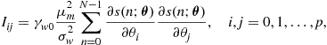
signal parameters from ![]() . Now, the elements of the Fisher information matrix
. Now, the elements of the Fisher information matrix ![]() are given by [35, Eqs. (4) and (5)]. Several foundational results are available in [35], including a polynomial signal model for
are given by [35, Eqs. (4) and (5)]. Several foundational results are available in [35], including a polynomial signal model for ![]() , as well as the iid non-Gaussian noise case (see Section 3.08.7.3).
, as well as the iid non-Gaussian noise case (see Section 3.08.7.3).
Specific signal models and estimators that have been addressed for the multiplicative and additive noise model include non-linear least squares estimation of sinusoids [36,37], the CRB for change point detection of a step-like signal [38], and Doppler shift [34,39]. Estimation of a single harmonic in multiplicative and additive noise arises in communications, radar, and other applications and has been studied extensively (e.g., see references in the above citations).
3.08.7.3 Non-Gaussian case
Next we consider the case when ![]() and
and ![]() in (8.27) may be non-Gaussian. While AWGN may always be present to some degree there are times when the central limit theorem is not applicable, such as a structured additive interference that is significantly non-Gaussian, and in such a case we might rely on a non-Gaussian pdf model for
in (8.27) may be non-Gaussian. While AWGN may always be present to some degree there are times when the central limit theorem is not applicable, such as a structured additive interference that is significantly non-Gaussian, and in such a case we might rely on a non-Gaussian pdf model for ![]() . For example, some electromagnetic interference environments are well modeled with a non-Gaussian pdf that has tails significantly heavier than Gaussian [40]. The study of the heavy-tailed non-Gaussian case is also strongly motivated to model the presence of outliers, leading to robust detection and estimation algorithms [41].
. For example, some electromagnetic interference environments are well modeled with a non-Gaussian pdf that has tails significantly heavier than Gaussian [40]. The study of the heavy-tailed non-Gaussian case is also strongly motivated to model the presence of outliers, leading to robust detection and estimation algorithms [41].
Let ![]() and
and ![]() denote the respective pdf’s of
denote the respective pdf’s of ![]() and
and ![]() in (8.27). Closed forms for
in (8.27). Closed forms for ![]() are typically not available, and it is difficult to obtain general results for the case when both
are typically not available, and it is difficult to obtain general results for the case when both ![]() and
and ![]() are present and at least one of them is non-Gaussian. However, following Swami [35], we can at least treat them separately as follows.
are present and at least one of them is non-Gaussian. However, following Swami [35], we can at least treat them separately as follows.
Consider (8.27) with ![]() a random constant so that
a random constant so that ![]() , and
, and ![]() . Let
. Let ![]() be a symmetric, not necessarily Gaussian pdf, and assume that
be a symmetric, not necessarily Gaussian pdf, and assume that ![]() is iid. Now, the FIM for
is iid. Now, the FIM for ![]() has elements given by [35, Eq. (21)]
has elements given by [35, Eq. (21)]
 (8.31)
where ![]() is the ith element of
is the ith element of ![]() , and we define [35, Eq. (20)]
, and we define [35, Eq. (20)]
 (8.32)
where x indicates the random variable with pdf ![]() , and k is integer with
, and k is integer with ![]() in (8.31). Thus the FIM
in (8.31). Thus the FIM ![]() depends on
depends on ![]() through its variance
through its variance ![]() and the value of
and the value of ![]() . In the Gaussian case
. In the Gaussian case ![]() , and (8.31) is well known, e.g., see Kay [42, Chapter 3]. For any symmetric
, and (8.31) is well known, e.g., see Kay [42, Chapter 3]. For any symmetric ![]() it follows that
it follows that ![]() , so that non-Gaussian
, so that non-Gaussian ![]() increases the Fisher information (i.e., lowers the CRB), and therefore AWGN is the worst case for estimating
increases the Fisher information (i.e., lowers the CRB), and therefore AWGN is the worst case for estimating ![]() . For example, the CRB for estimation of the parameters of an autoregressive process is minimized when the process is Gaussian [43]. On the other hand, it is often the case in practice with non-Gaussian noise that the exact form of the pdf is not known, so it may be necessary to estimate both the signal parameters and the parameters of a non-Gaussian pdf model.
. For example, the CRB for estimation of the parameters of an autoregressive process is minimized when the process is Gaussian [43]. On the other hand, it is often the case in practice with non-Gaussian noise that the exact form of the pdf is not known, so it may be necessary to estimate both the signal parameters and the parameters of a non-Gaussian pdf model.
The impact of non-Gaussian ![]() can be studied by setting
can be studied by setting ![]() . This purely multiplicative noise case has Fisher information given by [35, Eq. (25)]
. This purely multiplicative noise case has Fisher information given by [35, Eq. (25)]
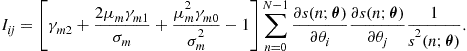 (8.33)
The FIM now depends on ![]() entirely through the first bracketed term in (8.33). This term is a function of the ratio
entirely through the first bracketed term in (8.33). This term is a function of the ratio ![]() , and
, and ![]() . Note that information is lost when
. Note that information is lost when ![]() , and that large
, and that large ![]() is desired to increase the FIM. Intuitively, when
is desired to increase the FIM. Intuitively, when ![]() , then the observed random fluctuation in
, then the observed random fluctuation in ![]() is reduced. When
is reduced. When ![]() is Gaussian, then
is Gaussian, then ![]() .
.
The preceding was limited to iid processes. The more general non-iid case is typically not very analytically tractable, because with dependence in ![]() or
or ![]() the joint pdf on all the observations is required, unlike the Gaussian case where second-order statistics are sufficient to characterize dependence. An exception is linear non-Gaussian processes, obtained as the output of a linear filter driven by an iid non-Gaussian random process. Here it may be of interest to identify the filter parameters [43], and if the filter is invertible then the problem can be returned to the iid case by a linear operation (whitening) [44,45]. Further discussion of non-iid issues in the non-Gaussian case is given by Poor and Thomas [46].
the joint pdf on all the observations is required, unlike the Gaussian case where second-order statistics are sufficient to characterize dependence. An exception is linear non-Gaussian processes, obtained as the output of a linear filter driven by an iid non-Gaussian random process. Here it may be of interest to identify the filter parameters [43], and if the filter is invertible then the problem can be returned to the iid case by a linear operation (whitening) [44,45]. Further discussion of non-iid issues in the non-Gaussian case is given by Poor and Thomas [46].
In our discussion around (8.27) we have largely focused on the signal parameters, but when we consider the non-Gaussian case we can also draw on the rich selection of parameterized non-Gaussian distributions. Well known families include Gaussian mixtures (GM) [47–50], stable distributions [51], and others [52].
The stable distributions include the normal distribution as a special limiting case, but otherwise have infinite variance. For almost all values of the stable distribution parameters simple closed form expressions are not available, with the notable exception of the Cauchy pdf. Consequently specialized tools and estimators have been developed for the case when ![]() is drawn from the stable distribution family, such as fractional lower order statistics, in order to accommodate the infinite variance of the pdf. For the case of linear (or iid) stable processes, normalized versions of conventional covariance and cumulant estimates are convergent and enable the use of many estimation algorithms originally developed for AWGN, e.g., covariance matrix based subspace algorithms [53,54].
is drawn from the stable distribution family, such as fractional lower order statistics, in order to accommodate the infinite variance of the pdf. For the case of linear (or iid) stable processes, normalized versions of conventional covariance and cumulant estimates are convergent and enable the use of many estimation algorithms originally developed for AWGN, e.g., covariance matrix based subspace algorithms [53,54].
CRBs are generally available for the cases mentioned here with additive iid non-Gaussian noise, using the expressions in [35]. Several cases are described in [50,55], generalizing the AWGN cases to non-Gaussian noise.
3.08.8 Asymptotic analysis and the central limit theorem
The CRB analysis above appeals to asymptotics, in the sense that the bound is generally tight only asymptotically, and application of the CRB requires a fully specified parametric probability model. However, we can often employ a more general asymptotic analysis without a parameteric model, and without completely specifying the pdf, by resorting to the central limit theorem (CLT) and related ideas. This approach is generally useful for analysis of algorithms. And, if there is an underlying parameteric model, then we can compare algorithm performance analysis with parameter estimation bounds such as the CRB. However, the asymptotic tools are general and apply even when there is no underlying parametric model. We consider the application of the CLT to two broad classes of algorithms in Section 3.08.9.
Given an estimation algorithm, a full statistical analysis requires the pdf of the estimate, as a function of the observations. If we know this pdf we can find meaningful measures of performance such as the mean, variance, and MSE, and compare these to benchmark bounds. We would like to do this as a function of the number of observations (data size), as well as other parameters such as the SNR. However, even if we have full statistical knowledge of the observations, it may be intractable to find the pdf of the estimates due to the often complicated and nonlinear estimation function.
An alternative approach is to appeal to asymptotics as the observation size grows [56]. The basic tools are two probability limit laws, (i) the law of large numbers (LLN) and (ii) the central limit theorem. The LLN reveals when a sample average of a sequence of n random variables converges to the expected mean as n goes to infinity, and the CLT tells us about the distribution of the sample average (or more generally about the distribution of a normalized sum of random variables).
The basic CLT theorem states that the sample average asymptotically converges in distribution to normal,
![]() (8.34)
(8.34)
where ![]() are iid,
are iid, ![]() , and Var
, and Var![]() . There are many extensions, such as the vector case, when the
. There are many extensions, such as the vector case, when the ![]() are non-identically distributed, and when the
are non-identically distributed, and when the ![]() are not independent. A generalized version of the CLT also exists for the non-Gaussian case with convergence to a stable distribution [57].
are not independent. A generalized version of the CLT also exists for the non-Gaussian case with convergence to a stable distribution [57].
Intuitively, when summing random variables, we recognize that the sum of independent random variables has pdf given by the convolution of the individual pdfs, and the repeated convolution results in smoothing to a Gaussian distribution. For example, suppose we average n random variables that are iid from a uniform distribution on ![]() . In this case
. In this case ![]() is sufficient to provide a very good fit to a normal distribution (up to the finite region of support of the ten-fold convolution) [58], so the asymptotics may be effective even for relatively small n in some cases.
is sufficient to provide a very good fit to a normal distribution (up to the finite region of support of the ten-fold convolution) [58], so the asymptotics may be effective even for relatively small n in some cases.
A physical intuition is also broadly applicable, that a combination of many small effects yields Gaussian behavior on the macro-scale, such as thermal noise in electronic devices resulting from electron motion.
3.08.8.1 Comments on application of the CLT
![]() Bounding asymptotic deviation from normality: The deviation of the asymptotic distribution from a normal pdf can be bounded. Perhaps the best known result is the Berry-Esséen theorem [56], that bounds the maximum deviation from Gaussian. The bound is proportional to
Bounding asymptotic deviation from normality: The deviation of the asymptotic distribution from a normal pdf can be bounded. Perhaps the best known result is the Berry-Esséen theorem [56], that bounds the maximum deviation from Gaussian. The bound is proportional to ![]() , the third central moment.
, the third central moment. ![]() is a measure of skewness of a pdf, i.e., it measures asymmetry in the pdf. If
is a measure of skewness of a pdf, i.e., it measures asymmetry in the pdf. If ![]() then the pdf is skewed left (e.g., has a heavier tail on left), and vice-versa. Generally then, asymmetry in the pdf of x will slow the asymptotic convergence to Gaussian.
then the pdf is skewed left (e.g., has a heavier tail on left), and vice-versa. Generally then, asymmetry in the pdf of x will slow the asymptotic convergence to Gaussian.
![]() Deviation from normality is generally worse in the tails of the pdf: The approximation to a normal process is generally more accurate when closer to the peak of the normal distribution, and may require a very large n for the fit to be accurate in the tails of the distribution. The fit between the distribution of the sample mean and its normal approximation worsens, at a given n, as we go out in the tails. This is intuitively evident in the example mentioned above, summing uniformly distributed random variables, because the convolution of multiple uniform pdfs will always have a finite support beyond which the true pdf is zero and so will always have error with respect to a normal distribution with it’s infinite support. Consequently, some care is needed when inferring from the tail behavior of the CLT Gaussian approximation. This is especially true in considering extreme tail behavior based on the form of the normal approximation, such as deriving tests of significance, confidence intervals (error bars), and rare events.
Deviation from normality is generally worse in the tails of the pdf: The approximation to a normal process is generally more accurate when closer to the peak of the normal distribution, and may require a very large n for the fit to be accurate in the tails of the distribution. The fit between the distribution of the sample mean and its normal approximation worsens, at a given n, as we go out in the tails. This is intuitively evident in the example mentioned above, summing uniformly distributed random variables, because the convolution of multiple uniform pdfs will always have a finite support beyond which the true pdf is zero and so will always have error with respect to a normal distribution with it’s infinite support. Consequently, some care is needed when inferring from the tail behavior of the CLT Gaussian approximation. This is especially true in considering extreme tail behavior based on the form of the normal approximation, such as deriving tests of significance, confidence intervals (error bars), and rare events.
![]() Applying the CLT to arbitrary functions: The various statements of the CLT usually stem from a (perhaps weighted) linear combination of random variables. However, in practice we are interested in applying the asymptotic theorem with empirical observations from an arbitrary function of the observations of the random variables, such as an estimator
Applying the CLT to arbitrary functions: The various statements of the CLT usually stem from a (perhaps weighted) linear combination of random variables. However, in practice we are interested in applying the asymptotic theorem with empirical observations from an arbitrary function of the observations of the random variables, such as an estimator ![]() . The CLT ideas are generally useful in this context when the estimator function stabilizes as n grows, i.e., given a sequence of random observations the estimator asymptotically converges to some value. If for large enough n then
. The CLT ideas are generally useful in this context when the estimator function stabilizes as n grows, i.e., given a sequence of random observations the estimator asymptotically converges to some value. If for large enough n then ![]() is reasonably Gaussian we can find its mean and variance, and the resulting normal distribution is a useful description of the pdf of the estimator. Note that, if we have a parametric model, then if
is reasonably Gaussian we can find its mean and variance, and the resulting normal distribution is a useful description of the pdf of the estimator. Note that, if we have a parametric model, then if ![]() is asymptotically normally distributed, is unbiased, and the variance approaches the CRB, then this estimator has asymptotic optimality. However, we stress that the CLT ideas are very general and don’t require an underlying parameteric model.
is asymptotically normally distributed, is unbiased, and the variance approaches the CRB, then this estimator has asymptotic optimality. However, we stress that the CLT ideas are very general and don’t require an underlying parameteric model.
![]() Tests for Gaussianity: Various statistical tests exist to determine if a random variable is well described by a Gaussian pdf, and these can and should be applied to verify the CLT effect in a particular case. For example, tests can be based on sample moments such as comparing the computed skewness and kurtosis with those expected for a normal distribution, as well as comparison through plots such as the Q-Q and P-P plots. Issues with such tests include obtaining sufficient data to accurately characterize the tail behavior, and that the test will provide some level of statistical evidence but not certainty.
Tests for Gaussianity: Various statistical tests exist to determine if a random variable is well described by a Gaussian pdf, and these can and should be applied to verify the CLT effect in a particular case. For example, tests can be based on sample moments such as comparing the computed skewness and kurtosis with those expected for a normal distribution, as well as comparison through plots such as the Q-Q and P-P plots. Issues with such tests include obtaining sufficient data to accurately characterize the tail behavior, and that the test will provide some level of statistical evidence but not certainty.
![]() Proving convergence to normality: Given an algorithm, we can rely on simulation and tests for Gaussianity to determine the validity of the asymptotic approximation. In general, it can be relatively difficult to prove convergence of the distribution of the output of a particular algorithm or estimator to normality. One approach is to show that the skewness and kurtosis converge to their expected values under a normal assumption (e.g., the skewness will approach zero because the normal distribution is symmetric). An example of this form of analysis is given by Brillinger, demonstrating that sample estimates of higher order statistics become normally distributed [59].
Proving convergence to normality: Given an algorithm, we can rely on simulation and tests for Gaussianity to determine the validity of the asymptotic approximation. In general, it can be relatively difficult to prove convergence of the distribution of the output of a particular algorithm or estimator to normality. One approach is to show that the skewness and kurtosis converge to their expected values under a normal assumption (e.g., the skewness will approach zero because the normal distribution is symmetric). An example of this form of analysis is given by Brillinger, demonstrating that sample estimates of higher order statistics become normally distributed [59].
3.08.9 Asymptotic analysis and parametric models
In the previous section we noted that asymptotic analysis of nonparametric algorithms is often facilitated by the law of large numbers and results associated with the central limit theorem. These ideas apply equally well to parameter estimators, even if we have the full parametric model specified in ![]() . While we may have the CRB or other bound that is applicable to a broad class of estimators, we would still like to carry out performance analysis for specific estimators, that may be the MLE or not.
. While we may have the CRB or other bound that is applicable to a broad class of estimators, we would still like to carry out performance analysis for specific estimators, that may be the MLE or not.
In this section we consider asymptotic analysis for two fundamentally important and widely applicable cases, Fourier based algorithms, and weighted least squares (LS) estimators. In both cases we can appeal to the CLT to show asymptotic normality, and then the algorithm performance can be characterized by the mean and covariance.
3.08.9.1 Fourier transform
The Fourier transform is a fundamental linear decomposition that can be exploited to facilitate performance analysis, because the transformation yields Fourier coefficients that tend to a complex-valued Gaussian distribution. The Fourier transform approach to analysis is particularly useful for wideband problems, such as wideband array processing [60], and bit error rate (BER) analysis of OFDM systems in a fading environment [61]. This represents an extremely small fraction of the literature using these ideas, and the basic concept can be readily extended to other signal decompositions.
We illustrate the idea in the following. Suppose we have observations from a random process ![]() , that depend on the deterministic parameters
, that depend on the deterministic parameters ![]() . We observe
. We observe ![]() over M intervals each of length T seconds. We may treat both the discrete-time and the continuous-time cases similarly. In discrete-time, samples
over M intervals each of length T seconds. We may treat both the discrete-time and the continuous-time cases similarly. In discrete-time, samples ![]() are placed in a vector and the DFT is applied. In continuous-time, we apply the short-time Fourier transform to obtain
are placed in a vector and the DFT is applied. In continuous-time, we apply the short-time Fourier transform to obtain
![]() (8.35)
(8.35)
over ![]() intervals, for
intervals, for ![]() distinct frequencies, and it is understood the integral is over successive time intervals of length T. We will drop the explicit mention of
distinct frequencies, and it is understood the integral is over successive time intervals of length T. We will drop the explicit mention of ![]() , keeping in mind the Fourier coefficients are functions of the parameters in the underlying pdf model that generates
, keeping in mind the Fourier coefficients are functions of the parameters in the underlying pdf model that generates ![]() . Asymptotically in T, the Fourier coefficients
. Asymptotically in T, the Fourier coefficients ![]() become normally distributed via the central limit theorem. In addition, in many cases, the
become normally distributed via the central limit theorem. In addition, in many cases, the ![]() become uncorrelated at different frequencies. This generally occurs when T is large compared to the time lag
become uncorrelated at different frequencies. This generally occurs when T is large compared to the time lag ![]() such that
such that ![]() and
and ![]() are weakly or completely uncorrelated, i.e.,
are weakly or completely uncorrelated, i.e., ![]() . For example, for a bandlimited random process with bandwidth B Hz, then the decorrelation time is roughly
. For example, for a bandlimited random process with bandwidth B Hz, then the decorrelation time is roughly ![]() .
.
Under the above assumptions, we place the ![]() complex-valued Fourier coefficients into L vectors
complex-valued Fourier coefficients into L vectors
![]() (8.36)
(8.36)
and let ![]() and
and ![]() be the mean and covariance matrix of
be the mean and covariance matrix of ![]() , respectively. Note that
, respectively. Note that ![]() describes the correlation at the frequency
describes the correlation at the frequency ![]() across time intervals; we are assuming that the Fourier coefficients are uncorrelated accross frequencies. Asymptotically the vectors
across time intervals; we are assuming that the Fourier coefficients are uncorrelated accross frequencies. Asymptotically the vectors ![]() are independent with a normal distribution, so the log-likelihood function can be written as
are independent with a normal distribution, so the log-likelihood function can be written as
 (8.37)
where H denotes conjugate-transpose (the Hermitian operator), and ![]() is the determinant. Recalling that
is the determinant. Recalling that ![]() and
and ![]() are functions of the parameters
are functions of the parameters ![]() , we can now use
, we can now use ![]() to find the MLE and CRB for estimation of
to find the MLE and CRB for estimation of ![]() . Note, however, that the MLE and CRB we are referring to are asymptotic approximations and were not derived directly from the original model.
. Note, however, that the MLE and CRB we are referring to are asymptotic approximations and were not derived directly from the original model.
If the original random process ![]() is Gaussian then the Fourier coefficients are also normally distributed because the Fourier transform is a linear operation. In this case, the only assumption leading to (8.37) is
is Gaussian then the Fourier coefficients are also normally distributed because the Fourier transform is a linear operation. In this case, the only assumption leading to (8.37) is ![]() , to ensure that the coefficients are uncorrelated at distinct frequencies. This does not require application of the CLT. More generally, if
, to ensure that the coefficients are uncorrelated at distinct frequencies. This does not require application of the CLT. More generally, if ![]() is non-Gaussian, then we rely on the CLT to ensure the Fourier coefficients are approaching a normal distribution. This depends on the observation interval length T (or equivalently the number of Nyquist samples when applying the DFT). For example, it is not difficult to accept that a DFT whose length is on the order of
is non-Gaussian, then we rely on the CLT to ensure the Fourier coefficients are approaching a normal distribution. This depends on the observation interval length T (or equivalently the number of Nyquist samples when applying the DFT). For example, it is not difficult to accept that a DFT whose length is on the order of ![]() or greater will produce a strong CLT effect.
or greater will produce a strong CLT effect.
As we noted in Section 3.08.8, it is important to validate the Gaussian assumption, such as using tests for Gaussianity as a function of the Fourier window time T. In addition, the assumption that the Fourier coefficients are uncorrelated should also be verified analytically or, e.g., using sample cross correlations. Note also that the Gaussian model can be readily modified to include frequency cross-correlation.
3.08.9.2 Least squares estimation
As a second example of the application of the CLT in parametric models, we consider weighted least squares nonlinear estimation, an extremely general tool. We will specifically assume the parameterized signal plus noise model in Eq. (8.1), where the noise is a stationary process with finite variance (not necessarily Gaussian). The least squares approach seeks to minimize the sum of squared errors criterion
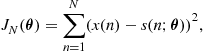 (8.38)
so that
![]() (8.39)
(8.39)
Unless ![]() is linear in
is linear in ![]() , then solving (8.39) is a nonlinear optimization problem. If the additive noise is Gaussian then (8.39) corresponds to maximum likelihood estimation, and we can appeal to classic CRB results, e.g., see [4]. If the noise pdf is unknown, then we cannot readily compute a CRB for estimation of
, then solving (8.39) is a nonlinear optimization problem. If the additive noise is Gaussian then (8.39) corresponds to maximum likelihood estimation, and we can appeal to classic CRB results, e.g., see [4]. If the noise pdf is unknown, then we cannot readily compute a CRB for estimation of ![]() .
.
The following is based on Wu [62]. Consider the parameterized signal plus additive noise model in (8.1). We assume that the additive noise is stationary with finite variance, but do not necessarily assume the noise pdf is known, nor do we assume the signal model is linear in the parameters ![]() . Putting the noisy observation into (8.38), the LS criterion seeks to fit the signal model to the noisy observations using the squared-error penalty for deviation from the model. This approach is very general and reasonable. Solution of (8.38) will require optimization, and with a nonlinear signal model there will generally be local optima, i.e., the cost function will not generally be convex. Thus the optimization algorithm may require search or a good initial estimate. For many examples of this scenario see Kay [4, Chapter 8]. Generally LS (or weighted LS) does not have any particular guaranteed finite sample optimality, but we can appeal to asymptotics.
. Putting the noisy observation into (8.38), the LS criterion seeks to fit the signal model to the noisy observations using the squared-error penalty for deviation from the model. This approach is very general and reasonable. Solution of (8.38) will require optimization, and with a nonlinear signal model there will generally be local optima, i.e., the cost function will not generally be convex. Thus the optimization algorithm may require search or a good initial estimate. For many examples of this scenario see Kay [4, Chapter 8]. Generally LS (or weighted LS) does not have any particular guaranteed finite sample optimality, but we can appeal to asymptotics.
Wu has shown the following asymptotic (as N grows) properties of LS for the case of a parametric signal in additive noise given by (8.1), resulting in (8.38). The LS estimator is consistent, i.e., it converges in probability to the true value of ![]() , meaning that the LS estimate has a probability distribution that is collapsing about the true value of
, meaning that the LS estimate has a probability distribution that is collapsing about the true value of ![]() . This assumes continuity in the pdf, and requires the LS error to grow with N except when the LS criterion is evaluated at the correct parameter. Intuitively, this last requirement implies that the signal does not die out. For example, suppose the signal undergoes an exponential decay. Then, the asymptotic properties are not guaranteed, but this is not surprising since the signal is dying off making additional observations of decreasing value. The signal must have sufficient energy and duration relative to the noise power for the asymptotic results to be meaningful. (Alternatively, we might have multiple observations of a finite length signal.)
. This assumes continuity in the pdf, and requires the LS error to grow with N except when the LS criterion is evaluated at the correct parameter. Intuitively, this last requirement implies that the signal does not die out. For example, suppose the signal undergoes an exponential decay. Then, the asymptotic properties are not guaranteed, but this is not surprising since the signal is dying off making additional observations of decreasing value. The signal must have sufficient energy and duration relative to the noise power for the asymptotic results to be meaningful. (Alternatively, we might have multiple observations of a finite length signal.)
The asymptotic results still hold when the noise is non-identically distributed (independent, but non-identical), so long as the variance is bounded. The same ideas hold even if the parameter ![]() is taken from a finite set, implying we are solving a classification problem rather than a continuous parameter estimation problem; see Section 3.08.2.1.5. Also, the average of the errors squared (the average sum of residuals squared) converges to the noise variance, so it is straightforward to asymptotically estimate the noise power.
is taken from a finite set, implying we are solving a classification problem rather than a continuous parameter estimation problem; see Section 3.08.2.1.5. Also, the average of the errors squared (the average sum of residuals squared) converges to the noise variance, so it is straightforward to asymptotically estimate the noise power.
Finally, note that the LS estimate is asymptotically normally distributed [62, Thrm. 5]. The variance of the normal distribution provides a large sample confidence level on the estimate of ![]() , which provides a probability statement about our confidence in a particular realization of the estimate, and this can be computed based on the observations. It is important to recognize that a confidence level provides statistical evidence, and should not be confused with a bound such as the CRB; see Section 3.08.11.
, which provides a probability statement about our confidence in a particular realization of the estimate, and this can be computed based on the observations. It is important to recognize that a confidence level provides statistical evidence, and should not be confused with a bound such as the CRB; see Section 3.08.11.
As with the Fourier case discussed previously, the validity of the asymptotic assumption should be carefully checked for a particular problem. For example, if the additive noise distribution strongly deviates from normal, or if there is significant dependence in the noise, then the convergence rate to the asymptotic regime may be slow.
3.08.10 Monte Carlo methods
A Monte Carlo method (MCM) is a computational algorithm that utilizes random sampling in some way during the computation, such as computing an expected value, where the algorithm uses realizations of some random process. This is a broad area of applications, and we consider some basic ideas as applied to performance analysis.
3.08.10.1 Using Monte Carlo to approximate an expectation
Consider numerically computing (or approximating) an expected value ![]() . As a simple example, suppose we wish to compute
. As a simple example, suppose we wish to compute ![]() , where x is a scalar random variable. We can generate many realizations of x and compute the sample average, which will converge to the expectation in most cases of interest based on the law of large numbers. Similar thinking applies to
, where x is a scalar random variable. We can generate many realizations of x and compute the sample average, which will converge to the expectation in most cases of interest based on the law of large numbers. Similar thinking applies to ![]() , for some function
, for some function ![]() ; generate realizations of x, and then compute the sample average of
; generate realizations of x, and then compute the sample average of ![]() . Because the expectation involves random variables, we can exploit random sampling in a straightforward averaging procedure. A particular motivation for MCM is when we are unable to carry out the expectation analytically. For example, the function
. Because the expectation involves random variables, we can exploit random sampling in a straightforward averaging procedure. A particular motivation for MCM is when we are unable to carry out the expectation analytically. For example, the function ![]() may be highly nonlinear such that no closed form is known for the expectation integral.
may be highly nonlinear such that no closed form is known for the expectation integral.
Thus we see that applying MCM is a fundamentally different sample-based approach to approximating the integral, as opposed to classic numerical methods such as using the trapezoidal rule. The integral may have infinite limits, and be of high dimension, cases that often confound classic numerical methods. Consequently, it may be more efficient and more accurate to employ MCM.
To reduce complexity, and to avoid excessive sampling in regions of small probability, additional sophistication can be employed in the sampling strategy; an example is importance sampling.
3.08.10.2 Computing the CRB via Monte Carlo
The MCM can be applied to numerically computing the CRB at a specified value of the parameter ![]() . Realizations of
. Realizations of ![]() are generated according to
are generated according to ![]() . These are then plugged into the Fisher score in (8.4), followed by averaging to estimate the FIM given by (8.3). Note that the averaging is over
. These are then plugged into the Fisher score in (8.4), followed by averaging to estimate the FIM given by (8.3). Note that the averaging is over ![]() for a fixed value of
for a fixed value of ![]() .
.
An alternative is to use the realizations of ![]() in (8.7). Note that in (8.7) the expectation is over the Hessian (the matrix of second derivatives). Thus, in this case, each realization of
in (8.7). Note that in (8.7) the expectation is over the Hessian (the matrix of second derivatives). Thus, in this case, each realization of ![]() results in a realization of the Hessian, and the Hessian matrices are averaged to approximate the FIM in (8.7).
results in a realization of the Hessian, and the Hessian matrices are averaged to approximate the FIM in (8.7).
Using either (8.3) or (8.7) assumes that the score or Hessian are known in closed form. If these derivatives are not known, then a Monte Carlo method may first be applied to estimate the derivatives for a given ![]() and
and ![]() . Then, these are averaged over the realizations
. Then, these are averaged over the realizations ![]() . This procedure is described in detail by Spall [16,63, chapter 12].
. This procedure is described in detail by Spall [16,63, chapter 12].
3.08.11 Confidence intervals
As described in Sections 3.08.8 and 3.08.9, in many cases we can exploit asymptotics to obtain an approximate (typically Gaussian) distribution for an estimate. For example, under the normal assumption, then an interval can be defined around the mean based on the variance ![]() of say,
of say, ![]() . While the mean of the distribution is our estimate, the variance provides a measure of confidence or reliability in the estimate, because it provides a statistical picture of the range over which the estimate might reasonably deviate given a new set of observations.
. While the mean of the distribution is our estimate, the variance provides a measure of confidence or reliability in the estimate, because it provides a statistical picture of the range over which the estimate might reasonably deviate given a new set of observations.
Note that the distribution parameters, and hence the confidence interval, are derived from the observations. So, the estimate and the confidence interval will change given a new set of observations. This should not be confused with a bound such as the CRB. The CRB is based on complete statistical knowledge of the underlying probability model ![]() .
.
Confidence intervals have been extensively applied in regression analysis, especially for additive Gaussian noise, but also more generally in the asymptotic sense with additive noise modeled as samples from an arbitrary stationary process. For example, see the comprehensive treatment by Draper and Smith [64].
An interesting alternative to estimating confidence levels is to use the bootstrap method; see Efron [65]. This approach does not rely on asymptotics, instead using resampling of the data. The approach is relatively simple to implement using the given observations, and does not require extensive knowledge of the underlying probability model, although it can be computationally demanding due to extensive resampling. An overview of the bootstrap in statistical signal processing is given by Zoubir [66].
3.08.12 Conclusion
We have introduced many key concepts in performance analysis for statistical signal processing. But of course, given the decades of developments in statistics and signal processing, there are many topics left untouched. These include treatment of random parameters, for example see the edited paper collection, Van Trees and Bell [67]. These are often referred to as Bayesian bounds. Alternatives to the CRB include the Ziv-Zakai bound [68,69], and the Chapman-Robbins bound [70]. These may be more challenging to derive analyically, but typically result in a tighter bound in the non-asymptotic region.
Relevant Theory: Signal Processing Theory, Machine Learning, and Statistical Signal Processing
See Vol. 1, Chapter 11 Parametric Estimation
See Vol. 1, Chapter 19 A Tutorial Introduction to Monte Carlo Methods, Markov Chain Monte Carlo and Particle Filtering
See Vol. 1, Chapter 25 Model Selection
See this Volume, Chapter 2 Model Order Selection
See this Volume, Chapter 4 Bayesian Computational Methods in Signal Processing
References
1. Shao Jun. Mathematical Statistics. New York, NY: Springer-Verlag; 2003.
2. Van Trees Harry L. Detection, Estimation, and Modulation Theory, Part I. Wiley 1968.
3. Casella George, Berger Roger L. Statistical Inference. second ed. Boca-Raton, FL: Duxbury Press; 2002.
4. Kay SM. Fundamentals of Statistical Signal Processing: Estimation Theory. Englewood Cliffs, NJ: Prentice Hall; 1993.
5. Cramér H. Mathematical Methods of Statistics. Princeton, NJ: Princeton University Press; 1946.
6. Radakrishna Rao Calyampudi. Information and the accuracy attainable in the estimation of statistical parameters. Bull Calcutta Math Soc. 1945;37:81–89.
7. Hero AO, Fessler JA, Usman M. Exploring estimator bias-variance tradeoffs using the uniform CR bound. IEEE Trans Signal Process. 1996;44(8):2026–2042.
8. A.O. Hero, J.A. Fessler, M. Usman, Bias-resolution-variance tradeoffs for single pixel estimation tasks using the uniform Cramér-Rao bound, in: Proc. of IEEE Nuclear Science, Symposium, vol. 2, pp. 296–298.
9. W.J. Bangs. Array processing with generalized beamformers. PhD Thesis, Yale University, New Haven, CT, 1971.
10. Slepian D. Estimation of signal parameters in the presence of noise. Trans IRE Prof Group Inform Theory PG IT-3 1954;68–69.
11. Rothenberg Thomas J. Identification in parametric models. Econometrica. 1971;39(3):577–591 May.
12. Hochwald B, Nehorai A. On identifiability and information-regularity in parameterized normal distributions. Circ Syst Signal Process. 1997;16(1):83–89.
13. Chen Y, Wiesel A, Eldar YC, Hero AO. Shrinkage algorithms for MMSE covariance estimation. IEEE Trans Signal Process. 2010;58(10):5016–5029.
14. Proakis JG, Salehi M. Digital Communications. fifth ed. McGraw-Hill 2007.
15. Simon MK, Alouini M-S. Digital Communications Over Fading Channels. second ed. Wiley 2005.
16. Spall JC. Introduction to Stochastic Search and Optimization. Wiley 2003.
17. Chen Y, Wiesel A, Hero AO. Robust shrinkage estimation of high dimensional covariance matrices. IEEE Trans Signal Process. 2011;59(9):4097–4107.
18. Liu N, Xu Z, Sadler BM. Geolocation performance with biased range measurements. IEEE Trans Signal Process. 2012;60(5):2315–2329.
19. Xu Z. Perturbation analysis for subspace decomposition with applications in subspace-based algorithms. IEEE Trans Signal Process. 2002;50(11):2820–2830.
20. Stewart GW. Error and perturbation bounds for subspaces associated with certain eigenvalue problems. SIAM Rev. 1973;15(4):727–764.
21. Stewart GW. On the perturbation of psuedo-inverses, projections and linear least squares problems. SIAM Rev. 1977;19(4):634–662.
22. Stewart GW, Sun J. Matric Perturbation Theory. Academic Press 1990.
23. Van Trees Harry L. Optimum Array Processing. Wiley 2002.
24. Li F, Liu H, Vaccaro RJ. Performance analysis for DOA estimation algorithms: unification, simplification, and observations. IEEE Trans Aerosp Electron Syst. 1993;29(4):1170–1184.
25. Weiss AJ, Picard J. Maximum-likelihood position estimation of network nodes using range measurements. IET Signal Process. 2008;2(4):394–404.
26. Stoica Petre, Chong Ng Boon. On the Cramér-Rao bound under parametric constraints. IEEE Signal Process Lett. 1998;5(7):177–179.
27. Moore Terrence J, Sadler Brian M. Sufficient conditions for regularity and strict identifiability in MIMO systems. IEEE Trans Signal Process. 2004;52(9):2650–2655.
28. Ben-Haim Zvika, Eldar Yonina. On the constrained Cramér-Rao bound with a singular Fisher information matrix. IEEE Signal Process Lett. 2009;16(6):453–456.
29. Moore Terrence J, Kozick Richard J, Sadler Brian M. The constrained Cramér-Rao bound from the perspective of fitting a model. IEEE Signal Process Lett. 2007;14(8):564–567.
30. Moore Terrence J, Sadler Brian M, Kozick Richard J. Maximum-likelihood estimation, the Cramér-Rao bound, and the method of scoring with parameter constraints. IEEE Trans Signal Process. 2008;56(3):895–908.
31. Rajasekaran PK, Satyanarayana N, Srinath MD. Optimum linear estimation of stochastic signals in the presence of multiplicative noise. IEEE Trans Aerosp Electron Syst. 1971;7(3):462–468.
32. Kozick RJ, Sadler BM, Wilson DK. Signal Processing and Propagation for Aeroacoustic Networks in Distributed Sensor Networks. CRC Press 2004.
33. Stoica Petre, Besson Olivier, Gershman Alex B. Direction-of-arrival estimation of an amplitude-distorted wavefront. IEEE Trans Signal Process. 2001;49(2):269–276.
34. Ghogho M, Swami A, Durrani TS. Frequency estimation in the presence of Doppler spread: performance analysis. IEEE Trans Signal Process. 2001;49(4):777–789.
35. Swami A. Cramer-Rao bounds for deterministic signals in additive and multiplicative noise. Signal Process. 1996;53:231–244.
36. Giannakis GB, Zhou G. Harmonics in Gaussian multiplicative and additive noise: Cramer-Rao bounds. IEEE Trans Signal Process. 1995;43(5):1217–1231.
37. Ghogho M, Swami A, Nandi AK. Non-linear least squares estimation for harmonics in multiplicative and additive noise. Signal Process. 1999;78:43–60.
38. Tourneret JY, Ferrari A, Swami A. Cramer-Rao lower bounds for change points in additive and multiplicative noise. Signal Process. 2004;84:1071–1088.
39. Ciblat P, Ghogho M, Forster P, Larzabal P. Harmonic retrieval in the presence of non-circular Gaussian multiplicative noise: performance bounds. Signal Process. 2005;85:737–749.
40. Middleton D, Spaulding AD. Elements of weak signal detection in non-gaussian noise environments. In: JAI Press 1993; Advances in Statistical Signal Processing. vol. 2.
41. Huber PJ, Ronchetti EM. Robust Statistics. second ed. Wiley 2009.
42. Kay SM. Fundamentals of Statistical Signal Processing: Estimation Theory. Prentice-Hall 1993.
43. Sengupta D, Kay S. Efficient estimation of parameters for a non-Gaussian autoregressive process. IEEE Trans Acoust Speech Signal Process. 1989;37(6):785–794.
44. Sadler BM, Giannakis GB, Lii K-S. Estimation and detection in non-Gaussian noise using higher order statistics. IEEE Trans Signal Process. 1994;42(10):2729–2741.
45. Sadler BM. Detection in correlated impulsive noise using fourth-order cumulants. IEEE Trans Signal Process. 1996;44(11):2793–2800.
46. Poor HV, Thomas JB. Signal detection in dependent non-gaussian noise. In: JAI Press 1993; Advances in Statistical Signal Processing. vol. 2.
47. Duda RO, Hart PE, Stork DG. Pattern Classification. second ed. Wiley 2001.
48. Kozick RJ, Blum RS, Sadler BM. Signal processing in non-Gaussian noise using mixture distributions and the EM algorithm. In: 1997;438–442. Proc 31st Asilomar Conference on Signals, Systems, and Computers. vol. 1.
49. Blum RS, Kozick RJ, Sadler BM. An adaptive spatial diversity receiver for non-gaussian interference and noise. IEEE Trans Signal Process. 1999;47(8):2100–2111.
50. Kozick RJ, Sadler BM. Maximum-likelihood array processing in non-Gaussian noise with Gaussian mixtures. IEEE Trans Signal Process. 2000;48(12):3520–3535.
51. Samorodnitsky G, Taqqu MS. Stable Non-Gaussian Random Processes: Stochastic Models with Infinite Variance. Chapman and Hall 1994.
52. Kassam SA, Thomas JB. Signal Detection in Non-Gaussian Noise. Springer 1987.
53. Davis RA, Resnick SI. Limit theory for the sample covariances and correlation functions of moving averages. Ann Stat. 1986;14:533–558.
54. Swami A, Sadler BM. On some detection and estimation problems in heavy-tailed noise. Signal Process. 2002;82:1829–1846.
55. Swami A, Sadler BM. Parameter estimation for linear alpha-stable processes. IEEE Signal Process Lett. 1998;5(2):48–50.
56. Serfling Robert J. Approximation Theorems of Mathematical Statistics. Wiley 1980.
57. Feller W. In: Wiley 1971; An Introduction to Probability Theory and Its Applications. vol. II.
58. Marsaglia G. Ratios of normal variables and ratios of sums of uniform variables. J Am Statist Assoc. 1965;60:193–204.
59. Brillinger DR, Rosenblatt M. Spectral analysis of time series. In: Harris B, ed. Asymptotic Theory of Estimates of k-th Order Spectra. Wiley 2002;153–188. Chapter 7.
60. Schultheiss PM, Messer H. Optimal and sub-optimal broad-band source location estimation. IEEE Trans Signal Process. 1993;41(9):2752–2763.
61. Siriwongpairat WP, Liu KJR. Ultra-Wideband Communications Systems. Wiley: IEEE Press; 2008.
62. Wu Chien-Fu. Asymptotic theory of nonlinear least squares estimation. Ann Stat. 1981;9(3):501–513.
63. Spall JC. On Monte Carlo methods for estimating the Fisher information matrix in difficult problems. In: 43rd Annual Conference on Information Sciences and Systems. 2009;741–746.
64. Draper NR, Smith H. Applied Regression Analysis. third ed. Wiley 1998.
65. Efron B, Tibshirani R. An Introduction to the Bootstrap. Chapman and Hall 1993.
66. Zoubir AM, Iskander DR. Bootstrap methods and applications. IEEE Signal Process Mag. 2007;24(4):10–19.
67. Van Trees HL, Bell KL. Bayesian Bounds for Parameter Estimation and Nonlinear/Filtering Tracking. IEEE Press, Wiley 2007.
68. Ziv J, Zakai M. Some lower bounds on signal parameter estimation. IEEE Trans Inform Theory 1969;386–391.
69. Chazan D, Zakai M, Ziv J. Improved lower bounds on signal parameter estimation. IEEE Trans Inform Theory. 1975;21(1):90–93.
70. Chapman DG, Robbins H. Minimum variance estimation without regularity assumptions. Ann Math Stat. 1951;22(6):581–586.