
Adaptive and Robust Beamforming*
Sergiy A. Vorobyov, Department of Signal Processing and Acoustics, Aalto University, FI-00076 AALTO, Finland and Department of Electrical and Computer Engineering, University of Alberta, Edmonton, AB T6G 2V4, Canada
Abstract
This chapter is dedicated to the overview of the main results in the fields of adaptive beamforming and robust adaptive beamforming. The basic principles and main approaches to adaptive and robust adaptive beamforming are explained based on the narrowband point source signal model. In addition, the extensions of the basic principles and approaches to the general rank source model and wideband signal are given. The particular numerical algorithms for adaptive beamforming such as the gradient algorithm, the sample matrix inversion algorithm, and the projection adaptive beamforming algorithm are reviewed. The particular robust adaptive beamforming techniques are the diagonally loaded sample matrix inversion beamforming technique, the robust adaptive beamforming techniques with point and derivative mainbeam constraints, the generalized sidelobe canceler, the adaptive beamforming techniques robust against the correlation between the signal of interest and interferences such as spatial and forward-backward smoothing, the adaptive beamforming techniques robust against rapidly moving interferences, the eigenspace-based beamforming technique, the worst-case-based and doubly constrained robust adaptive beamforming techniques, the probabilistically constrained robust adaptive beamforming technique, the robust adaptive beamforming that uses as little as possible prior information, and others.
Keywords
Adaptive beamforming; Robustness; Array processing; Convex optimization
Acknowledgments
The author of this chapter would like to acknowledge the input of Prof. Alex B. Gershman (formerly of Darmstadt University of Technology, Germany). While still alive, Prof. Gershman has shared with the author some materials on adaptive beamforming including a number of figures used in this chapter. Without these figures, the presentation would be significantly less illustrative.
3.12.1 Introduction
Adaptive beamforming is a versatile approach to detect and estimate the signal-of-interest (SOI) at the output of sensor array using data adaptive spatial or spatio-temporal filtering and interference cancellation [1–3]. Being a very central problem of array processing (see [4]), adaptive beamforming has found numerous application to radar [5,6], sonar [7], speech processing [8], radio astronomy [9,10], biomedicine [11,12], wireless communications [13–15], cognitive communications [16], and other fields. The connection of adaptive beamforming to adaptive filtering is emphasized in [4]. The major differences, however, come from the fact that adaptive filtering is based on temporal processing of a signal, while adaptive beamforming stresses on spatial processing. The latter indicates also that the signal is sampled in space, i.e., the signal is measured/observed by an array of spatially distributed antenna elements/sensors. Electronic beamforming design problem consists of computing optimal (in some sense that will be specified) complex beamforming weights for sensor measurements of the signal. If such complex beamforming weights are optimized based on the input/output array data/measurements, the corresponding beamforming is called adaptive to distinguish it from the conventional beamforming where the beamforming weights do not depend on input/output array data.
The traditional approach to the design of adaptive beamforming is to maximize the beamformer output signal-to-interference-plus-noise ratio (SINR) assuming that there is no SOI component in the beamforming training data [2,3]. Although such SOI-free data assumption may be relevant to certain radar applications, in typical practical applications, the beamforming training snapshots also include the SOI [17,18]. In the latter case, the SINR performance of adaptive beamforming can severely degrade even in the presence of small signal steering vector errors/mismatches, because the SOI component in the beamformer training data can be mistakenly interpreted by the adaptive beamforming algorithm as an interferer and, consequently, it can be suppressed rather than being protected. The steering vector errors are, however, very common in practice and can be caused by a number of reasons such as signal look direction/pointing errors; array calibration imperfections; non-linearities in amplifiers, A/D converters, modulators and other hardware; distorted antenna shape; unknown wavefront distortions/fluctuations; signal fading; near-far wavefront mismodeling; local scattering; and many other effects. The performance degradation of adaptive beamformer can also take place even when the SOI steering vector is precisely known, but the sample size (the number of samples at the training stage) is small [18]. One more reason for performance degradation is the environmental non-stationarities because of the fast variations of the propagation channel and rapid motion of interfering sources or antenna array [19]. As a result, the environment can significantly change from the beamforming training stage, at which the adaptive beamforming weights are computed, to the beamforming testing stage, at which the beamforming weights are used. This may severely limit the training sample size and increase the required frequency of beamforming weights updates. To protect against the aforementioned imperfections, the robust adaptive beamforming is considered.
This chapter is dedicated to the review of the main results in the fields of adaptive beamforming and robust adaptive beamforming. We start by introducing the array data and beamforming models for both cases on narrowband and wideband signals. Adaptive beamforming techniques are then reviewed including the basic principles of adaptive beamforming design, minimum variance distortionless response adaptive beamforming technique, analysis of optimal SINR, adaptive beamforming technique for general rank sources. The general numerical algorithms for solving the adaptive beamforming problem such as the gradient algorithm, the sample matrix inversion algorithm, and the projection adaptive beamforming algorithm are also reviewed. Finally, the reduced complexity approaches to adaptive beamforming and some techniques for wideband adaptive beamforming are explained. The motivations for robust adaptive beamforming then follow. The particular robust adaptive beamforming techniques explained in this chapter include the diagonally loaded sample matrix inversion beamforming technique, the robust adaptive beamforming techniques with point and derivative mainbeam constraints, the generalized sidelobe canceler, the adaptive beamforming techniques robust against the correlation between the SOI and interferences such as spatial and forward-backward smoothing, the adaptive beamforming techniques robust against rapidly moving interferences. A unified principle to minimum variance distortionless response robust adaptive beamforming design is given and several most popular robust adaptive beamforming techniques based on this principle are explained including the eigenspace-based beamforming technique, the worst-case-based and doubly constrained robust adaptive beamforming techniques, the probabilistically constrained robust adaptive beamforming, and the recently proposed robust adaptive beamforming that uses as little as possible prior information, and others. Robust adaptive beamforming for general-rank source model and robust adaptive wideband beamforming are also considered.
3.12.2 Data and beamforming models
In this chapter, the discussion is focussed on adaptive and robust adaptive beamforming and is based on the assumptions of linear antenna geometry consisting of omni-directional antenna elements. Other considerations, which are not directly related to the adaptive beamforming problem, such as non-linear multi-dimensional antenna geometries and antenna elements with directional beampattern stay outside of the scope of this chapter.
3.12.2.1 Narrowband case
3.12.2.1.1 Point source
Consider an antenna array with M omni-directional antenna elements see also the introduction to array processing in this encyclopedia [4]. The narrowband signal received by the antenna array at the time instant k can be mathematically represented as
![]() (12.1)
(12.1)
where ![]() , and
, and ![]() denote the
denote the ![]() vectors of the SOI, interference, and noise, respectively. The interference signal is generated by other than SOI sources that are not of interest (interferers and possibly a jammer). For simplicity, all these components of the received signal (12.1) are assumed to be statistically independent to each other. This assumption is fairly practical since the SOI and the signals from interferers (other objects or users) are typically independent. The case of correlated/coherent SOI and interference signals, however, can occur in practice, for example, because of the scattering effect. This case will be considered separately in the chapter as well. The noise is typically isotropic or diffuse and it can be accurately modeled as spatially white Gaussian noise (i.e., the noise components are spatially uncorrelated at different antenna elements with the same noise power at each antenna element). In other words, the
vectors of the SOI, interference, and noise, respectively. The interference signal is generated by other than SOI sources that are not of interest (interferers and possibly a jammer). For simplicity, all these components of the received signal (12.1) are assumed to be statistically independent to each other. This assumption is fairly practical since the SOI and the signals from interferers (other objects or users) are typically independent. The case of correlated/coherent SOI and interference signals, however, can occur in practice, for example, because of the scattering effect. This case will be considered separately in the chapter as well. The noise is typically isotropic or diffuse and it can be accurately modeled as spatially white Gaussian noise (i.e., the noise components are spatially uncorrelated at different antenna elements with the same noise power at each antenna element). In other words, the ![]() covariance matrix of the noise at the antenna array can be expressed as
covariance matrix of the noise at the antenna array can be expressed as ![]() , where
, where ![]() is the noise variance/power at a single antenna element,
is the noise variance/power at a single antenna element, ![]() denotes the identity matrix of the same size as the number of antenna elements in the array, and
denotes the identity matrix of the same size as the number of antenna elements in the array, and ![]() and
and ![]() stand for the Hermitian transpose and mathematical expectation, respectively. As such, the noise is statistically independent from the SOI and interference signals.
stand for the Hermitian transpose and mathematical expectation, respectively. As such, the noise is statistically independent from the SOI and interference signals.
In the case of point source, it is assumed that the SOI ![]() arrives at the antenna array as a single plane wave and it can be mathematically represented as
arrives at the antenna array as a single plane wave and it can be mathematically represented as
![]() (12.2)
(12.2)
where ![]() is the signal waveform,
is the signal waveform, ![]() is the
is the ![]() steering vector associated with the SOI, and
steering vector associated with the SOI, and ![]() is the direction-of-arrival (DOA) of the SOI. Although the steering vector
is the direction-of-arrival (DOA) of the SOI. Although the steering vector ![]() is expressed only as a function of the DOA
is expressed only as a function of the DOA ![]() , which is the source characteristic in the case of far distant point source, one should keep in mind that it is in fact also a function of array geometry as well as propagation media characteristics. The covariance matrix of the SOI for the case of point source can be, therefore, expressed in the form of the following
, which is the source characteristic in the case of far distant point source, one should keep in mind that it is in fact also a function of array geometry as well as propagation media characteristics. The covariance matrix of the SOI for the case of point source can be, therefore, expressed in the form of the following ![]() rank-one matrix:
rank-one matrix: ![]() , where
, where ![]() is the SOI power.
is the SOI power.
The beamformer output is a weighted (with complex weights) linear combination of the signals received by different antenna elements (see also Figure 1.3 in Chapter 1 of this book [4]) at the time instant k and it can be mathematically expressed as
 (12.3)
where ![]() is the complex weight corresponding to the mth antenna element,
is the complex weight corresponding to the mth antenna element, ![]() in the signal received by the mth antenna element at the time instant
in the signal received by the mth antenna element at the time instant ![]() is the
is the ![]() complex weight (beamforming) vector of the antenna array, and
complex weight (beamforming) vector of the antenna array, and ![]() and
and ![]() denote the transpose and conjugate, respectively. The expression (12.3) is in fact a linear spatial filter. The beamforming complex weights
denote the transpose and conjugate, respectively. The expression (12.3) is in fact a linear spatial filter. The beamforming complex weights ![]() can be applied to the signals received by the correspondent antenna elements right at these antenna elements or at the receiver electronics. The weights
can be applied to the signals received by the correspondent antenna elements right at these antenna elements or at the receiver electronics. The weights ![]() must be designed so that the SOI would be presumed/amplified at the beamformer output, the interference signals would be canceled, and the noise would be suppressed.
must be designed so that the SOI would be presumed/amplified at the beamformer output, the interference signals would be canceled, and the noise would be suppressed.
If only the SOI component is present, the beamformer output in the case of point source becomes ![]() . From the latter expression the interpretation of the beamformer in terms of a special filter becomes intuitive. Indeed,
. From the latter expression the interpretation of the beamformer in terms of a special filter becomes intuitive. Indeed, ![]() can be thought as the spatial transfer function from
can be thought as the spatial transfer function from ![]() at the direction
at the direction ![]() to
to ![]() . The magnitude
. The magnitude ![]() is the gain of the spatial filter towards the SOI. It is similar to the finite impulse response (FIR) filtering in the temporal domain where instead of the spatial steering vector
is the gain of the spatial filter towards the SOI. It is similar to the finite impulse response (FIR) filtering in the temporal domain where instead of the spatial steering vector ![]() we have a vector of time-delayed values of the input signal. For more details see the introduction to array processing in this encyclopedia [4].
we have a vector of time-delayed values of the input signal. For more details see the introduction to array processing in this encyclopedia [4].
Under the assumption that the SOI steering vector ![]() is known precisely, the optimal beamforming vector
is known precisely, the optimal beamforming vector ![]() can be obtained by maximizing the beamformer output signal-to-noise-plus-interference ratio (SINR) given as
can be obtained by maximizing the beamformer output signal-to-noise-plus-interference ratio (SINR) given as
 (12.4)
where ![]() is the
is the ![]() interference-plus-noise covariance matrix.
interference-plus-noise covariance matrix.
Because of the fact that ![]() is unknown in practice, it is typically substituted in (12.4) by the following data sample covariance matrix
is unknown in practice, it is typically substituted in (12.4) by the following data sample covariance matrix
 (12.5)
where K is the number of training data samples which also include the desired signal component. Other estimates of the data covariance matrix than (12.5) can be used [20]. It is worth mentioning here that since the noise is spatially white Gaussian and uncorrelated with the SOI and interference signals, the actual data covariance matrix can be found as
![]() (12.6)
(12.6)
where ![]() is the
is the ![]() matrix of steering vectors of the SOI and the interference sources under the assumption that all sources are the point sources, L is the number of interference sources,
matrix of steering vectors of the SOI and the interference sources under the assumption that all sources are the point sources, L is the number of interference sources, ![]() is the
is the ![]() source covariance matrix. The matrix
source covariance matrix. The matrix ![]() is diagonal if the SOI and all interference signals are uncorrelated.
is diagonal if the SOI and all interference signals are uncorrelated.
3.12.2.1.2 General-rank source
Typical situations in practice, however, are when the source signal is incoherently scattered (spatially distributed) [21,22] and/or when it is characterized by fluctuating (randomly distorted) wavefronts [23,24]. Such situations are very typical, for example, for sonar and wireless communications. Particularly in sonar, effects of signal propagation through a randomly inhomogeneous underwater channel lead to a substantial perturbation of a regular wakefield in a random way and cause its coherence loss. The result of such coherence loss is that the SOI may be subject to fast fluctuations that destroy the point source structure (12.2). In wireless communications, the common situation is the fast fading due to local scattering in the vicinity of the mobile user. Local scattering also destroys the point source structure (12.2). In such applications, the SOI can no longer be viewed by the antenna array as a point source and the source model needs to be modified. Typically, the SOI is modeled as a spatially distributed source with some central angle and angular spread. The source covariance matrix is, therefore, no longer a rank-one matrix and, for example, in the incoherently scattered source case can be given as [25]
![]() (12.7)
(12.7)
where ![]() is the normalized angular power density (i.e.,
is the normalized angular power density (i.e., ![]() ). The name “general rank source” is reflecting the fact that the covariance matrix (12.7) can have any rank from 1 in a degenerate case to M.
). The name “general rank source” is reflecting the fact that the covariance matrix (12.7) can have any rank from 1 in a degenerate case to M.
In the case of general-rank SOI, the SINR expression is given as
![]() (12.8)
(12.8)
Since the matrix ![]() is not known in practice it is substituted by the data sample covariance matrix (12.5) in practice.
is not known in practice it is substituted by the data sample covariance matrix (12.5) in practice.
3.12.2.2 Wideband case
In the wideband case, the SOI and/or the interference signals are widely spread in the frequency domain. As a result, it is not possible to factorize the processing in temporal and spatial parts. Therefore, joint space-time adaptive processing (STAP) has to be performed. The name STAP stresses on the fact that the adaptive beamforming in the wideband case is no longer a spatial filtering technique as for the narrowband case, but rather a joint spatial and temporal filtering. For more details see the chapter on broadband beamforming in this encyclopedia [26].
Let the number of taps in the time domain be denoted as P. Let also the M array sensors be uniformly spaced with the inter-element spacing less than or equal to ![]() , where
, where ![]() is the maximum frequency of the SOI/maximum passband frequency,
is the maximum frequency of the SOI/maximum passband frequency, ![]() is the carrier frequency,
is the carrier frequency, ![]() is the signal bandwidth, and c is the wave propagation speed. The general case of not necessarily uniform linear array (ULA) is considered in a specialized chapter on broadband beamforming of this encyclopedia [26]. The received signal at the mth antenna element goes to a wideband presteering delay filter with the delay
is the signal bandwidth, and c is the wave propagation speed. The general case of not necessarily uniform linear array (ULA) is considered in a specialized chapter on broadband beamforming of this encyclopedia [26]. The received signal at the mth antenna element goes to a wideband presteering delay filter with the delay ![]() . Let the output of the wideband presteering delay filter be sampled with the sampling frequency
. Let the output of the wideband presteering delay filter be sampled with the sampling frequency ![]() , where
, where ![]() in the sampling time and
in the sampling time and ![]() is greater than or equal to
is greater than or equal to ![]() . Then the
. Then the ![]() stacked snapshot vector containing P delayed presteered data vectors is the data vector
stacked snapshot vector containing P delayed presteered data vectors is the data vector ![]() . The beamformer output
. The beamformer output ![]() is then given by [27]
is then given by [27]
![]() (12.9)
(12.9)
where ![]() is the real-valued
is the real-valued ![]() beamformer weight vector, i.e.,
beamformer weight vector, i.e., ![]() and, thus,
and, thus, ![]() is equivalently substituted by
is equivalently substituted by ![]() .
.
In the wideband case, the steering vector also depends on frequency and in the case of a ULA is given as
![]() (12.10)
(12.10)
where ![]() is the mth antenna element location that for ULA is given as
is the mth antenna element location that for ULA is given as ![]() with d denoting the inter-element spacing. The overall
with d denoting the inter-element spacing. The overall ![]() steering vector can be expressed as
steering vector can be expressed as
![]() (12.11)
(12.11)
where ![]() , and
, and ![]() denotes the Kronecker product. Then the array response to a plane wave with the frequency f and angle or arrival
denotes the Kronecker product. Then the array response to a plane wave with the frequency f and angle or arrival ![]() is
is
![]() (12.12)
(12.12)
The presteering delays are selected so that the SOI arriving from the look direction ![]() appears coherently at the output of the M presteering filters so that [27]
appears coherently at the output of the M presteering filters so that [27]
![]() (12.13)
(12.13)
where ![]() is the
is the ![]() vector containing all ones. Then the steering vector towards the look direction
vector containing all ones. Then the steering vector towards the look direction ![]() becomes
becomes
![]() (12.14)
(12.14)
and the array response towards such signal becomes
![]() (12.15)
(12.15)
where ![]() .
.
3.12.3 Adaptive beamforming
3.12.3.1 Basic principles
The signal-to-noise ratio (SNR) gain due to coherent processing of the signal ![]() received at the antenna array, i.e., due to receive beamforming, is proportional to the quantity
received at the antenna array, i.e., due to receive beamforming, is proportional to the quantity ![]() in the case of a point source. Here
in the case of a point source. Here ![]() is the presumed SOI DOA. Using the Cauchy-Schwarz inequality, it can be easily found that
is the presumed SOI DOA. Using the Cauchy-Schwarz inequality, it can be easily found that ![]() , where equality holds when
, where equality holds when
![]() (12.16)
(12.16)
The expression (12.16) is referred to as the conventional nonadaptive beamforming. In the case when a single point source signal is observed in the background of white Gaussian noise, the conventional nonadaptive beamformer (12.16) is known to be optimal in the sense that it provides the highest possible output SNR gain [3]. The idealistic condition of a single point source (no interferences) is, however, impractical. Moreover, the precise estimate of the SOI steering vector ![]() is required in (12.16). In the presence of interferences, (12.16) is no longer optimal and, thus, adaptive beamforming technique are of interest.
is required in (12.16). In the presence of interferences, (12.16) is no longer optimal and, thus, adaptive beamforming technique are of interest.
The goal of adaptive beamforming as a spatial adaptive filter is to filter out (suppress) the undesired interference and noise components ![]() and
and ![]() as much as possible, and to detect and obtain as good as possible approximation/estimation of the desired signal
as much as possible, and to detect and obtain as good as possible approximation/estimation of the desired signal ![]() , the estimate is denoted as
, the estimate is denoted as ![]() . The beamforming weight vector
. The beamforming weight vector ![]() is optimized based on the received data
is optimized based on the received data ![]() for a number of time instants
for a number of time instants ![]() during the training interval. Since the adaptive beamforming problem consists of optimizing the beamforming weight vector
during the training interval. Since the adaptive beamforming problem consists of optimizing the beamforming weight vector ![]() , the optimization criterion must be defined.
, the optimization criterion must be defined.
One of the standard in filter design and estimation theory criteria is the mean-square error (MSE). In the context of adaptive beamforming design, the MSE criterion can be expressed as
![]() (12.17)
(12.17)
where ![]() is the desired signal copy. The corresponding optimization problem is then formulated as follows:
is the desired signal copy. The corresponding optimization problem is then formulated as follows:
![]() (12.18)
(12.18)
The solution of the minimum MSE problem is well known to be the Wiener-Hopf equation, which for the optimization problem (12.18) becomes
![]() (12.19)
(12.19)
where ![]() is the data covariance matrix and
is the data covariance matrix and ![]() in the correlation vector between the data vector
in the correlation vector between the data vector ![]() and the reference signal d.
and the reference signal d.
The block scheme of the adaptive beamformer based on MSE minimization (12.19) is shown in Figure 12.1. The adaptive beamformer consists of the “master” and “slave” beamformers. The beamforming weights are adjusted at the “master” beamformer based on minimizing the difference between the desired signal copy and the computed (using the antenna array measurements) output of the adaptive beamformer. These weights are then passed to the “slave” beamformer for computing the estimate of the desired signal ![]() . The main limitation of such adaptive beamformer is the necessity to know the desired signal copy
. The main limitation of such adaptive beamformer is the necessity to know the desired signal copy ![]() . In Figure 12.1, this necessity is reflected by introducing the generator of desired signal copy. Although the knowledge of the desired signal copy is common in adaptive filtering, in adaptive beamforming the SOI is unknown. Thus, the adaptive beamformer based on MSE minimization is impractical in most of the situations of interest.
. In Figure 12.1, this necessity is reflected by introducing the generator of desired signal copy. Although the knowledge of the desired signal copy is common in adaptive filtering, in adaptive beamforming the SOI is unknown. Thus, the adaptive beamformer based on MSE minimization is impractical in most of the situations of interest.

The practically appealing criterion for adaptive beamforming design is the SINR (12.4) for the case of a point source or (12.8) for the case of a general-rank source. Obviously, the SINR does not depend on re-scaling of the beamforming vector ![]() , that is, if
, that is, if ![]() is an optimal weight vector then
is an optimal weight vector then ![]() is another optimal weight vector as well. Here
is another optimal weight vector as well. Here ![]() is a scaling factor. Therefore, in the case of point source, the maximization of the SINR (12.4) is equivalent to the following constrained optimization problem
is a scaling factor. Therefore, in the case of point source, the maximization of the SINR (12.4) is equivalent to the following constrained optimization problem
![]() (12.20)
(12.20)
where “![]() ” is any constant, for example,
” is any constant, for example, ![]() . The optimization problem (12.20) and its solution are known under the name of minimum variance distortionless response (MVDR) adaptive beamforming. Here the “minimum variance” stands for the fact that the objective of the optimization problem (12.20) corresponds to the variance minimization of the signal at the output of the adaptive beamformer. The term “distortionless response” refers to the constraint of the optimization problem (12.20), which requires the response of the adaptive beamformer towards the direction of the SOI steering vector
. The optimization problem (12.20) and its solution are known under the name of minimum variance distortionless response (MVDR) adaptive beamforming. Here the “minimum variance” stands for the fact that the objective of the optimization problem (12.20) corresponds to the variance minimization of the signal at the output of the adaptive beamformer. The term “distortionless response” refers to the constraint of the optimization problem (12.20), which requires the response of the adaptive beamformer towards the direction of the SOI steering vector ![]() to be fixed and undistorted.
to be fixed and undistorted.
The optimization problem (12.20) can be solved in closed-form using the Lagrange multiplier method. Specifically, the Lagrangian for the problem (12.20) is given as
![]() (12.21)
(12.21)
where ![]() is a Lagrange multiplier. The solution of (12.20) is then obtained by finding the gradient of the Lagrangian (12.21), equating it to zero, and solving the so-obtained equation. This equation is
is a Lagrange multiplier. The solution of (12.20) is then obtained by finding the gradient of the Lagrangian (12.21), equating it to zero, and solving the so-obtained equation. This equation is
![]() (12.22)
(12.22)
and it can be rewritten equivalently as
![]() (12.23)
(12.23)
Then, the solution of (12.23) can be easily found as
![]() (12.24)
(12.24)
This is a spatial version of the Wiener-Hopf equation. Compared to (12.19), there is the SOI spatial signature/steering vector ![]() in (12.24) instead of the correlation vector
in (12.24) instead of the correlation vector ![]() . Moreover, there is the interference-plus-noise covariance matrix
. Moreover, there is the interference-plus-noise covariance matrix ![]() instead of the data covariance matrix
instead of the data covariance matrix ![]() . The Lagrange multiplier
. The Lagrange multiplier ![]() can be easily found by substituting (12.24) in the distortionless response constraint of the original optimization problem (12.20) and solving the corresponding equation for
can be easily found by substituting (12.24) in the distortionless response constraint of the original optimization problem (12.20) and solving the corresponding equation for ![]() . The result is
. The result is
![]() (12.25)
(12.25)
Finally, substituting (12.25) in (12.24), the closed-form expression for the MVDR beamforming can be obtained in the following form:
![]() (12.26)
(12.26)
The block scheme of the adaptive beamformer based on SINR maximization is shown in Figure 12.2. According to this block scheme, the beamforming weights are computed at the adaptive processor, which implements the estimation of the covariance matrix ![]() and then computes the beamforming weight vector according to (12.26). The input data for the adaptive processor are the antenna array measurements
and then computes the beamforming weight vector according to (12.26). The input data for the adaptive processor are the antenna array measurements ![]() , while the output, which is passed to the antenna elements, is the vector of optimal beamforming weights
, while the output, which is passed to the antenna elements, is the vector of optimal beamforming weights ![]() . If the received signal is free of the desired signal component, the sample estimate of the covariance matrix
. If the received signal is free of the desired signal component, the sample estimate of the covariance matrix ![]() can be obtained based on the expression (12.5). Otherwise, only the sample estimate of the data covariance matrix
can be obtained based on the expression (12.5). Otherwise, only the sample estimate of the data covariance matrix ![]() can be found by using (12.5). The latter case when the signal of interest is present in the data vector
can be found by using (12.5). The latter case when the signal of interest is present in the data vector ![]() is, however, common in practice.
is, however, common in practice.

3.12.3.2 MVDR beamforming with data covariance matrix
Even if the SOI is present in the data vector ![]() , but the estimate of the data covariance matrix is perfect and the steering vector of the SOI
, but the estimate of the data covariance matrix is perfect and the steering vector of the SOI ![]() is known precisely, the resulting beamformer that uses the data covariance matrix instead of the interference-plus-noise covariance matrix is equivalent to the MVDR beamformer of (12.26). Indeed, the data covariance matrix in the case of point source can be represented by explicitly using the interference-plus-noise covariance matrix as
is known precisely, the resulting beamformer that uses the data covariance matrix instead of the interference-plus-noise covariance matrix is equivalent to the MVDR beamformer of (12.26). Indeed, the data covariance matrix in the case of point source can be represented by explicitly using the interference-plus-noise covariance matrix as
![]() (12.27)
(12.27)
Ignoring the immaterial for the SINR at the output of the adaptive beamformer coefficient ![]() in (12.26), using the data covariance matrix (12.27) instead of the interference-plus-noise covariance matrix, and applying consequently the matrix inversion lemma, it can be shown that
in (12.26), using the data covariance matrix (12.27) instead of the interference-plus-noise covariance matrix, and applying consequently the matrix inversion lemma, it can be shown that
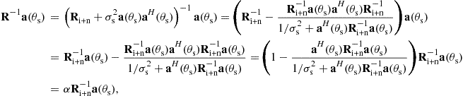 (12.28)
where the coefficient ![]() is immaterial for the output SINR of the adaptive beamformer.
is immaterial for the output SINR of the adaptive beamformer.
3.12.3.3 Optimal SINR
The optimal output SINR is the maximum SINR obtained by substituting the optimal MVDR beamforming vector (12.26) in the SINR expression (12.4). Specifically, the optimal SINR in the case of a point source is given by
 (12.29)
The expression (12.29) is in fact an upper bound for the output SINR, obtained for the case of no interference.
For rough estimation of the optimal SINR in the case when there are only a few uncorrelated interferences and the signal is well separated from them, the interference-plus-noise covariance matrix can be approximated by a scaled identity matrix with a scaling coefficient representing the aggregate power of the interferences and noise denoted as ![]() . Then the upper bound for the optimal SINR (12.29) is
. Then the upper bound for the optimal SINR (12.29) is
![]() (12.30)
(12.30)
where for obtaining the last equality, the fact that the squared norm of the steering vector equals to the number of sensors in the antenna array, i.e., ![]() , has been used. Thus, roughly, the optimal SINR is upper bounded by the product of the input SINRs at the individual antenna elements and the total number of antenna elements in the antenna array.
, has been used. Thus, roughly, the optimal SINR is upper bounded by the product of the input SINRs at the individual antenna elements and the total number of antenna elements in the antenna array.
3.12.3.4 Adaptive beamforming for general-rank source
In the case of general-rank source, the SINR expression (12.8) is the one that has to be used. The corresponding MVDR-type optimization problem can be then formulated as
![]() (12.31)
(12.31)
The solution of the optimization problem (12.31) is well known to be the principal eigenvector of the matrix product ![]() , that is mathematically expressed as
, that is mathematically expressed as
![]() (12.32)
(12.32)
where ![]() denotes the operator that computes the principal eigenvector of a matrix. The solution (12.32) is of a limited practical use because in most applications, the matrix
denotes the operator that computes the principal eigenvector of a matrix. The solution (12.32) is of a limited practical use because in most applications, the matrix ![]() is unknown, and often no reasonable estimate of it is available. However, if the estimate of
is unknown, and often no reasonable estimate of it is available. However, if the estimate of ![]() is available as well as the estimate of
is available as well as the estimate of ![]() , (12.32) provides a simple solution to the adaptive beamforming problem for the general-rank source. The solution of (12.32) can be equivalently found as the solution of the characteristic equation for the matrix
, (12.32) provides a simple solution to the adaptive beamforming problem for the general-rank source. The solution of (12.32) can be equivalently found as the solution of the characteristic equation for the matrix ![]() , that is,
, that is, ![]() , if the matrix
, if the matrix ![]() is full-rank invertible. In practice, however, the rank of the desired source can be smaller than the number of sensors in the antenna array and the source covariance matrix
is full-rank invertible. In practice, however, the rank of the desired source can be smaller than the number of sensors in the antenna array and the source covariance matrix ![]() may not be invertible, while the matrix
may not be invertible, while the matrix ![]() is guaranteed to be invertible due to the presence of the noise component. Therefore, the solution (12.32) is always preferred practically.
is guaranteed to be invertible due to the presence of the noise component. Therefore, the solution (12.32) is always preferred practically.
3.12.3.5 Gradient adaptive beamforming algorithms
The interference-plus-noise and data covariance matrices are unknown in practice. Assuming that there is a finite number of training snapshots ![]() that do not contain the SOI component and that the SOI steering vector
that do not contain the SOI component and that the SOI steering vector ![]() is known precisely, the historically first adaptive beamforming method is the gradient algorithm developed back in the 1960s of the last century [28]. Similar to the least-mean square (LMS) adaptive filtering, the gradient adaptive beamforming algorithm can be mathematically expresed as
is known precisely, the historically first adaptive beamforming method is the gradient algorithm developed back in the 1960s of the last century [28]. Similar to the least-mean square (LMS) adaptive filtering, the gradient adaptive beamforming algorithm can be mathematically expresed as
![]() (12.33)
(12.33)
where ![]() stands for the beamforming weight vector at the kth iteration, i.e., after processing the kth data snapshot, and
stands for the beamforming weight vector at the kth iteration, i.e., after processing the kth data snapshot, and ![]() is the step size of the LMS algorithm. The convergence condition for the gradient adaptive beamforming algorithm is similar to that of the LMS convergence condition and is formulated as follows. The beamforming vector
is the step size of the LMS algorithm. The convergence condition for the gradient adaptive beamforming algorithm is similar to that of the LMS convergence condition and is formulated as follows. The beamforming vector ![]() converges to the MVDR beamforming solution (12.26) if
converges to the MVDR beamforming solution (12.26) if
![]() (12.34)
(12.34)
where ![]() denotes the maximum eigenvalue of a square matrix. Finding the maximum eigenvalue required in (12.34) is computationally complex. Hence, using the property that the maximum eigenvalue of a positive semi-definite square matrix is smaller or equal to the trace of such matrix, (12.34) can be simplified as
denotes the maximum eigenvalue of a square matrix. Finding the maximum eigenvalue required in (12.34) is computationally complex. Hence, using the property that the maximum eigenvalue of a positive semi-definite square matrix is smaller or equal to the trace of such matrix, (12.34) can be simplified as
![]() (12.35)
(12.35)
where ![]() stands for the trace of a square matrix.
stands for the trace of a square matrix.
The covariance matrix ![]() is, however, not known in practice. Thus, the choice of the step size
is, however, not known in practice. Thus, the choice of the step size ![]() that guarantees the convergence of the algorithm (12.33) is a nontrivial practical issue. Another main disadvantage of the gradient adaptive beamforming algorithm is that the convergence depends on eigenvalue spread of the matrix
that guarantees the convergence of the algorithm (12.33) is a nontrivial practical issue. Another main disadvantage of the gradient adaptive beamforming algorithm is that the convergence depends on eigenvalue spread of the matrix ![]() and may be very slow. To demonstrate it, the following simulation example is considered.
and may be very slow. To demonstrate it, the following simulation example is considered.
A ULA consists of ![]() omni-directional sensors spaced half-wavelength apart from each other. A single SOI impinges on the antenna array form the direction
omni-directional sensors spaced half-wavelength apart from each other. A single SOI impinges on the antenna array form the direction ![]() with
with ![]() dB, while a single interference impinges on the antenna array form the direction
dB, while a single interference impinges on the antenna array form the direction ![]() with interference-to-noise ratio
with interference-to-noise ratio ![]() dB. The gradient adaptive beamforming algorithm (12.33) is tested for three different values of the step size:
dB. The gradient adaptive beamforming algorithm (12.33) is tested for three different values of the step size: ![]() , and
, and ![]() . The results are shown in Figure 12.3 which demonstrates the convergence of (12.33) for different values of
. The results are shown in Figure 12.3 which demonstrates the convergence of (12.33) for different values of ![]() in terms of the output SINR in (dB) versus the number of snapshots, i.e., the number of algorithm iterations. The optimal SINR (12.29) that provides an absolute upper bound for the output SINR of an adaptive beamformer is also shown. It can be seen from Figure 12.3 that the convergence is faster for larger
in terms of the output SINR in (dB) versus the number of snapshots, i.e., the number of algorithm iterations. The optimal SINR (12.29) that provides an absolute upper bound for the output SINR of an adaptive beamformer is also shown. It can be seen from Figure 12.3 that the convergence is faster for larger ![]() , but the variance of the output SINR values distribution is significantly higher compared to the case of small
, but the variance of the output SINR values distribution is significantly higher compared to the case of small ![]() . Moreover, even in the case of fastest convergence, the number of iterations required for convergence, i.e., the required number of training snapshots is well above 1000 which is too large number in most practical applications. As an extreme example, in radar field only a single snapshot may be available.
. Moreover, even in the case of fastest convergence, the number of iterations required for convergence, i.e., the required number of training snapshots is well above 1000 which is too large number in most practical applications. As an extreme example, in radar field only a single snapshot may be available.

3.12.3.6 Sample matrix inversion adaptive beamformer
The sample matrix inversion (SMI) adaptive beamformer [29] is obtained by replacing the interference-plus-noise covariance matrix ![]() in the MVDR beamformer (12.26) with the sample estimate of the data covariance matrix (12.5). Then the expression for the corresponding beamformer is given as
in the MVDR beamformer (12.26) with the sample estimate of the data covariance matrix (12.5). Then the expression for the corresponding beamformer is given as
![]() (12.36)
(12.36)
Under the assumption shared by all traditional adaptive beamforming techniques that the SOI component is not present in the training data, the requirement of the SMI beamformer on the number of training snapshots is given by the so-called Reed-Mallett-Brennan (RMB) rule [29]. It states that the mean losses (relative to the optimal SINR) due to the SMI approximation of ![]() (12.26) do not exceed 3 dB if
(12.26) do not exceed 3 dB if
![]() (12.37)
(12.37)
Hence, the SMI beamformer has in general fast convergence rate that is much faster than that of the gradient adaptive bemforming algorithm.
3.12.3.7 Projection adaptive beamforming methods
Although the RMB rule for the SMI beamformer provides a significantly faster convergence rate compared to the gradient adaptive beamforming algorithm, the number of required training snapshots may be still quite significant especially for large arrays. The so-called Hung-Turner or projection adaptive beamformer allows to reduce the number of training snapshots even further [30].
Under the standard for traditional adaptive beamforming techniques assumption that the SOI component is not present in the training data and also under the assumption that the noise power is negligible, the inverse of the data covariance matrix ![]() can be closely approximated by the orthogonal projection matrix
can be closely approximated by the orthogonal projection matrix ![]() where the matrix
where the matrix ![]() in the absence of the SOI becomes
in the absence of the SOI becomes ![]() , i.e., it only consists of L interference steering vectors. The interference steering vectors are unknown in practice and, thus,
, i.e., it only consists of L interference steering vectors. The interference steering vectors are unknown in practice and, thus, ![]() is also unknown. However, under the aforementioned assumptions of no SOI and negligible noise power,
is also unknown. However, under the aforementioned assumptions of no SOI and negligible noise power, ![]() can be closely approximated by the data-orthogonal projection matrix
can be closely approximated by the data-orthogonal projection matrix ![]() , where
, where ![]() is the matrix of available training snapshots. Thus, the following train of approximate equalities holds:
is the matrix of available training snapshots. Thus, the following train of approximate equalities holds:
![]() (12.38)
(12.38)
Replacing ![]() in (12.26) by the data-orthogonal projection matrix as in (12.38), the Hung-Turner adaptive beamforming algorithm can be written as
in (12.26) by the data-orthogonal projection matrix as in (12.38), the Hung-Turner adaptive beamforming algorithm can be written as
![]() (12.39)
(12.39)
For this method, a satisfactory performance can be achieved with [30]
![]() (12.40)
(12.40)
The optimal value of K is [30]
![]() (12.41)
(12.41)
which may be significantly smaller than the value given by the RMB rule for the SMI beamformer especially for large antenna arrays and for the scenarios with small number of interferences. The drawback of the projection adaptive beamformer is, however, that the number of interference sources should be known a priori.
3.12.3.8 Reduced complexity approaches to adaptive beamforming
The Hung-Turner adaptive beamforming algorithm (12.39) is especially efficient when the number of sensors in the array is much larger than the number of interferences. However, in some applications the number of sensors in the array, or equivalently, the number of adaptive degrees of freedom (adaptive beamforming weights) is so large that the computational complexity of the beamformer (12.39) becomes high. For example, the over-the-horizon radar may consists of hundreds and thousands of antenna elements [31], while the number of interferences may be relatively few. In such cases, partially adaptive arrays can be used to reduce the amount of computations [3].
The idea of partially adaptive array is to use nonadaptive (data-independent) preprocessor to reduce the number of adaptive channels. Mathematically, such nonadaptive preprocessor can be expressed as
![]() (12.42)
(12.42)
where ![]() is an
is an ![]()
![]() fixed preprocessing full-rank matrix and
fixed preprocessing full-rank matrix and ![]() has a reduced dimension of
has a reduced dimension of ![]() relative to
relative to ![]() for the original data vector
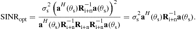
for the original data vector ![]() . The block scheme of the partially adaptive beamformer is shown in Figure 12.4 where the M measurements of the antenna array are first preprocessed by multiplying the vector
. The block scheme of the partially adaptive beamformer is shown in Figure 12.4 where the M measurements of the antenna array are first preprocessed by multiplying the vector ![]() to the preprocessing matrix
to the preprocessing matrix ![]() . Then the adaptive beamformer is applied to the preprocessed vector
. Then the adaptive beamformer is applied to the preprocessed vector ![]() .
.
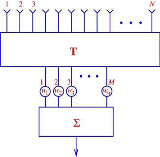
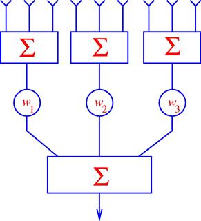
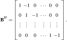
There are two type of preprocessors: subarray preprocessing and beamspace preprocessing. An example of partially adaptive beamformer with subarray preprocessor is shown in Figure 12.5. In this example, the matrix ![]() takes a form of
takes a form of
 (12.43)
It can be easily seen that ![]() for (12.43). It is a desired property since the preprocessing may lead to colored noise if
for (12.43). It is a desired property since the preprocessing may lead to colored noise if ![]() . However, the noise remains spatially white if
. However, the noise remains spatially white if ![]() .
.
The preprocessing of type (12.43) or a general preprocessing that follows (12.42) changes the array manifold. We say that the element-space of the antenna array is transformed into the beam-space of a smaller dimension to stress on the fact that the resulting array manifold is changed and, thus, the new SOI steering vector is
![]() (12.44)
(12.44)
The relationship between the element-space and beam-space is also shown in Figure 12.6 for a certain partially adaptive beamformer based on subarray preprocessing. For an arbitrary preprocessor, the covariance matrix of the preprocessed data ![]() can be expressed as
can be expressed as
![]() (12.45)
(12.45)
Substituting the expression (12.6) for the actual data covariance matrix in (12.45), we obtain
![]() (12.46)
(12.46)
where
![]() (12.47)
(12.47)
![]() (12.48)
(12.48)
and the noise covariance matrix for the preprocessed data ![]() may not be a scaled identity matrix in general. Thus, while designing the preprocessing matrix the condition
may not be a scaled identity matrix in general. Thus, while designing the preprocessing matrix the condition
![]() (12.49)
(12.49)
has to be ensured.
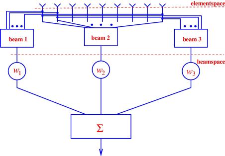
Figure 12.6 Element-space and beam-space of a partially adaptive beamformer based on subarray preprocessing.
Existing designs for the preprocessing matrix ![]() that satisfy the condition (12.49) are the discrete Fourier transform (DFT)-based beamspace preprocessing technique and the spheroidal sequences technique [3,32,33]. Both techniques consider an angular sector
that satisfy the condition (12.49) are the discrete Fourier transform (DFT)-based beamspace preprocessing technique and the spheroidal sequences technique [3,32,33]. Both techniques consider an angular sector ![]() where the SOI is likely to be located, i.e.,
where the SOI is likely to be located, i.e., ![]() , and attempt to design a set of vectors that are orthonormal in this sector. Such orthonormal vectors form the preprocessing matrix
, and attempt to design a set of vectors that are orthonormal in this sector. Such orthonormal vectors form the preprocessing matrix ![]() and guarantee that the property (12.49) is satisfied.
and guarantee that the property (12.49) is satisfied.
The DFT-based beamspace preprocessing matrix is expressed as
![]() (12.50)
(12.50)
where all vectors are DFT orthonormal vectors covering the angular sector ![]() with an angular sampling interval
with an angular sampling interval ![]() .
.
The essence of the spheroidal sequence technique [33] to the design of the preprocessing matrix ![]() (beamspace transformation) [32] is to take the principal eigenvectors of the matrix
(beamspace transformation) [32] is to take the principal eigenvectors of the matrix
![]() (12.51)
(12.51)
as columns of ![]() . Since these columns are the eigenvectors, they will be orthonormal as desired.
. Since these columns are the eigenvectors, they will be orthonormal as desired.
3.12.3.9 Wideband adaptive beamforming
One popular approach to wideband beamforming is to decompose the baseband waveforms into narrowband frequency components by the means of fast Fourier transform (FFT) [34,35]. Subsequently, the subbands can be processed independently from each other using narrowband beamforming techniques as it is shown in Figure 12.7. Then any of the above discussed adaptive beamforming methods can be used to solve each narrowband beamforming problem. Thus, P adaptive beamforming problems, each for the beamforming vector of length M, are needed to be solved. The time-domain beamformer output samples are obtained by applying an inverse FFT (IFFT) of the output samples of the individual narrowband beamformers. However, such FFT-based wideband beamforming technique is not optimal, since correlations between the frequency domain snapshot vectors of different subbands are not taken into account. Although these correlations can be reduced by increasing the FFT length, the latter requires a larger training data set [34].
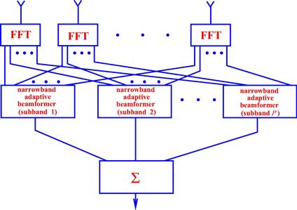
Based on the wideband data and beamforming models introduced in Section 3.12.2.2, another approach to wideband beamforming that does not require subband decomposition has been developed [27]. The block scheme of such adaptive beamformer is shown in Figure 12.8. As explained in Section 3.12.2.2, this beamformer uses a presteering delay front-end consisting of presteering delay filters to time-align the desired signal components in different sensors. Then the presteering delays are followed by FIR filters, each of length P. The beamformer output is then the sum of the filtered waveforms. The weights of such spatial-temporal filter for the wideband MVDR beamformer are designed to minimize the output power subject to the distortionless response constraint for the SOI. Multiple mainbeam constraints are required to protect the SOI in the frequency band of interest. The distortionless response constraint is formulated for the steering vector (12.14) after the SOI components in different sensors are made identical at the presteering stage. Then the narrowband adaptive beamforming algorithms introduced in this section can be extended relatively straightforwardly for the STAP shown in Figure 12.8. Moreover, the so-called generalized sidelobe canceler-type of techniques that will be explained in Section 3.12.4.4 can be straightforwardly used [27]. For more details and designs for wideband adaptive beamforming see also the specialized chapter on broadband beamforming in this encyclopedia [26].

3.12.4 Robust adaptive beamforming
3.12.4.1 Motivations
The result (12.28) on the equivalence between the MVDR adaptive beamformer with the interference-to-noise covariance matrix and the one with the data covariance matrix holds true only under the conditions that
• there is infinite number of snapshots available at the training stage and the data covariance matrix can be estimated exactly or at least with high accuracy,
However, these conditions are not satisfied in practice since the data covariance matrix ![]() cannot be known exactly and its estimate
cannot be known exactly and its estimate ![]() typically contains the SOI component where the desired signal steering vector
typically contains the SOI component where the desired signal steering vector ![]() may be known imprecisely. The applications where the SOI component is always present in the training data include mobile communications, passive source location, microphone array speech processing, medical imaging, radio astronomy, etc. The inaccuracies in the knowledge of the SOI steering vector may appear for multiple reasons associated with imperfect knowledge of the source characteristics, propagation media or antenna array itself. For example, even small look direction/signal pointing errors can lead to significant degradation of the adaptive beamformer performance [36,37]. Similarly, an imperfect array calibration and distorted antenna shape can also lead to significant degradations [38]. Other common causes of the adaptive beamformer’s performance degradation are the array manifold mismodeling due to source wavefront distortions resulting from environmental inhomogeneities [39], nea-far problem [40], source spreading and local scattering [41–43], and so on.
may be known imprecisely. The applications where the SOI component is always present in the training data include mobile communications, passive source location, microphone array speech processing, medical imaging, radio astronomy, etc. The inaccuracies in the knowledge of the SOI steering vector may appear for multiple reasons associated with imperfect knowledge of the source characteristics, propagation media or antenna array itself. For example, even small look direction/signal pointing errors can lead to significant degradation of the adaptive beamformer performance [36,37]. Similarly, an imperfect array calibration and distorted antenna shape can also lead to significant degradations [38]. Other common causes of the adaptive beamformer’s performance degradation are the array manifold mismodeling due to source wavefront distortions resulting from environmental inhomogeneities [39], nea-far problem [40], source spreading and local scattering [41–43], and so on.
All the aforementioned issues are addressed in the field of robust adaptive beamforming. One of the earlier excellent reviews of the field is [44]. However, many new techniques and approaches have been developed since this review. This section aims at revising the most significant robust adaptive beamforming techniques.
3.12.4.2 Diagonally loaded SMI beamformer
Even in the ideal case when the SOI steering vector is precisely known, the SOI presence in the training data may dramatically reduce the convergence rates of adaptive beamforming algorithms as compared with the SOI-free training data case [18]. This may cause a much more substantial degradation of the performance of adaptive beamforming techniques in situations of small training sample size compared to the prediction given, for example, by the RMB rule (12.37) for the SMI adaptive beamformer (12.36).
By adding a regularization term in the objective function of the optimization problem (12.20) that penalizes the imperfections in the data covariance matrix estimate due to small sample size and other effects, the problem (12.20) can be reformulated as
![]() (12.52)
(12.52)
where ![]() is some penalty parameter. The solution to the problem (12.52) is given by the well known diagonally loaded or shortly just loaded SMI (LSMI) beamformer [17,45,46]
is some penalty parameter. The solution to the problem (12.52) is given by the well known diagonally loaded or shortly just loaded SMI (LSMI) beamformer [17,45,46]
![]() (12.53)
(12.53)
where the empirically-optimal penalty weight ![]() equals to double the noise power [17]. LSMI beamformer allows to converge faster than in
equals to double the noise power [17]. LSMI beamformer allows to converge faster than in ![]() snapshots suggested by the RMB rule.
snapshots suggested by the RMB rule.
LSMI convergence rule: the mean losses (relative to the optimal SINR) due to the LSMI approximation of ![]() in (12.26) do not exceed a few dB’s if
in (12.26) do not exceed a few dB’s if
![]() (12.54)
(12.54)
Interestingly, for properly selected ![]() , the LSMI beamformer is also efficient in the case when the desired signal steering vector is mismatched. This fact will be explained in details later. However, the choice of
, the LSMI beamformer is also efficient in the case when the desired signal steering vector is mismatched. This fact will be explained in details later. However, the choice of ![]() is not a trivial problem for the LSMI beamformer. Another important observation is that the convergence rule for the LSMI beamformer coincides with that of the Hung-Turner beamformer. Thus, the Hung-Turner beamformer can also be classified as robust against small sample size.
is not a trivial problem for the LSMI beamformer. Another important observation is that the convergence rule for the LSMI beamformer coincides with that of the Hung-Turner beamformer. Thus, the Hung-Turner beamformer can also be classified as robust against small sample size.
To demonstrate the efficiency of the LSMI beamformer compared to the SMI beamformer, the following simulation example is considered. A ULA consists of 10 omni-directional sensors spaced half wavelength apart from each other. The DOA of a single SOI is ![]() and
and ![]() dB, while the DOA of a single interference is
dB, while the DOA of a single interference is ![]() and
and ![]() dB. Figures 12.9 and 12.10 show the beampatterns of the SMI and LSMI beamformers, respectively. The number of training snapshots for the SMI beamformer equals to
dB. Figures 12.9 and 12.10 show the beampatterns of the SMI and LSMI beamformers, respectively. The number of training snapshots for the SMI beamformer equals to ![]() that satisfies the RMB rule (12.37), while the number of training snapshots for the LSMI beamformer equals only
that satisfies the RMB rule (12.37), while the number of training snapshots for the LSMI beamformer equals only ![]() that satisfies the LSMI convergence rule (12.54). It can be seen from the figures that despite the fact that the number of training snapshots for the LSMI beamformer is 10 times smaller than that for the SMI beamformer, the beampattern corresponding to the LSMI beamformer has a significantly higher mainlobe and lower sidelobes. The parameter
that satisfies the LSMI convergence rule (12.54). It can be seen from the figures that despite the fact that the number of training snapshots for the LSMI beamformer is 10 times smaller than that for the SMI beamformer, the beampattern corresponding to the LSMI beamformer has a significantly higher mainlobe and lower sidelobes. The parameter ![]() for the LSMI beamformer has been selected as double the noise power.
for the LSMI beamformer has been selected as double the noise power.

Figure 12.9 Beampattern of the SMI beamformer for the number of snapshots ![]() that satisfies the RMB rule (12.37).
that satisfies the RMB rule (12.37).

Figure 12.10 Beampattern of the LSMI beamformer for the number of snapshots ![]() that satisfies the LSMI convergence rule (12.54).
that satisfies the LSMI convergence rule (12.54).
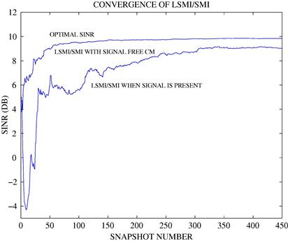
In addition, Figure 12.11 demonstrates the convergence rate for the SMI beamformer for two cases when the SOI component is not present in the training snapshots and when it is present. The same simulation set up as above has been used. It can be seen from this figure that the presence of the SOI component in the training snapshots significantly slows down the convergence of the SMI beamformer. The same conclusion is true for the LSMI beamformer with fixed diagonal loading factor ![]() that is selected as double the noise power.
that is selected as double the noise power.
3.12.4.3 Look direction mismatch (pointing error) problem
Although the mismatch in the desired signal steering vector can be caused by a number of reasons, the look direction mismatch (pointing error) has been considered historically first. Even a very slight look direction mismatch can lead to the effect that is known as the signal cancellation phenomenon. This phenomenon is schematically demonstrated in Figure 12.12 where the presumed DOA of the SOI differs from the real DOA by few degrees. The adaptive beamformer misinterprets the desired signal with an interference and puts the null in the direction of the SOI. The signal cancellation phenomenon may cause a performance breakdown for adaptive beamformer and, thus, robust adaptive beamforming techniques become vital.
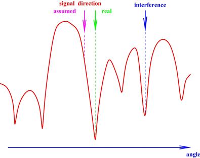
Figure 12.12 Look direction mismatch (pointing error) problem. The SOI arrives from a different direction than the presumed direction.
To stabilize the mainbeam response of adaptive beamformer in the case of pointing error, additional constraints are required. If all additional constraints are of the same type as the destortionless response constraint, i.e., linear constraints, the optimization problem can be reformulated as
![]() (12.55)
(12.55)
where ![]() and
and ![]() are some
are some ![]() and
and ![]() matrix and vector, respectively. Depending on the choice of
matrix and vector, respectively. Depending on the choice of ![]() or
or ![]() , we may have point or derivative mainbeam constraints [27,47].
, we may have point or derivative mainbeam constraints [27,47].
Point mainbeam constraints: In this case, the matrix of constrained directions is given as
![]() (12.56)
(12.56)
where ![]() are all taken in the neighborhood of the steering vector in the presumed direction
are all taken in the neighborhood of the steering vector in the presumed direction ![]() and include the steering vector in the presumed direction as well. Then the vector of constraints
and include the steering vector in the presumed direction as well. Then the vector of constraints ![]() is
is
![]() (12.57)
(12.57)
The constraint in the optimization problem (12.55) consists of multiple point constraints similar to the distortionless response constraints, but covers not only the presumed direction, but also the directions in the neighborhood of the presumed direction. The work principle of the point mainlobe constraint is demonstrated in Figure 12.13.

The disadvantage of using multiple distortionless response constraints is that additional degrees of freedom are used by the beamformer in order to satisfy these constraints. Since for an antenna array of M sensors, the number of degrees of freedom is M, the use of each additional degree of freedom for satisfying additional distortionless response constraints limits the remaining degrees of freedom that may be needed for suppressing interference signals.
Derivative mainbeam constraints: In this case, the matrix of constrained directions is given as
 (12.58)
and the vector of constraints is
![]() (12.59)
(12.59)
Here
 (12.60)
where ![]() is the matrix that depends on the SOI presumed DOA
is the matrix that depends on the SOI presumed DOA ![]() and the array geometry.
and the array geometry.
The solution of the optimization problem can be found in a similar way as the solution of the MVDR beamformer, and it can be written as
![]() (12.61)
(12.61)
Since the data covariance matrix is unknown in practice, its sample estimate has to be used. Then the SMI version of the beamformer (12.61) is
![]() (12.62)
(12.62)
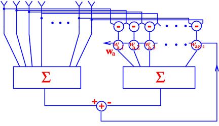
3.12.4.4 Generalized sidelobe canceler
The solution (12.61) can be decomposed into two components, one in the constrained subspace and the other in the orthogonal subspace to the constrained subspace, as follows [27]:
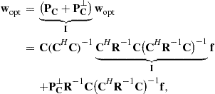 (12.63)
where ![]() and
and ![]() are the projection matrix on the constrained subspace and the orthogonal projection matrix on the constrained subspace, respectively.
are the projection matrix on the constrained subspace and the orthogonal projection matrix on the constrained subspace, respectively.
The decomposition (12.63) can be written in a general form as
![]() (12.64)
(12.64)
where
![]() (12.65)
(12.65)
is the so-called quiescent beamforming vector, which is independent of the input/output data of the antenna array. The matrix ![]() in (12.64) must be selected so that
in (12.64) must be selected so that
![]() (12.66)
(12.66)
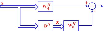
and it is called the blocking matrix. The vector ![]() is the new adaptive weight vector, while
is the new adaptive weight vector, while ![]() is non-adaptive. The beamformer (12.64) is called the generalized sidelobe canceler (GSC). Its block scheme is shown in Figure 12.14 and it consists of the non-adaptive branch and adaptive branch, in which the adaptive beamforming vector is applied to the data vector
is non-adaptive. The beamformer (12.64) is called the generalized sidelobe canceler (GSC). Its block scheme is shown in Figure 12.14 and it consists of the non-adaptive branch and adaptive branch, in which the adaptive beamforming vector is applied to the data vector ![]() after the blocking matrix
after the blocking matrix ![]() that blocks the constrained directions.
that blocks the constrained directions.
The choice of the blocking matrix ![]() in the GSC (12.64) is not unique. In (12.63), for example, the blocking matrix
in the GSC (12.64) is not unique. In (12.63), for example, the blocking matrix ![]() is used. However, in this case,
is used. However, in this case, ![]() is not a full-rank matrix. Therefore, it is more common to select an
is not a full-rank matrix. Therefore, it is more common to select an ![]() full-rank matrix
full-rank matrix ![]() . Then, the vectors
. Then, the vectors ![]() and
and ![]() both have shorter length of
both have shorter length of ![]() relative to the
relative to the ![]() vectors
vectors ![]() and
and ![]() . Since the non-adaptive component
. Since the non-adaptive component ![]() is data independent and has to be pre-computed only once, the GSC reduces the computational complexity by requiring to compute only the adaptive component
is data independent and has to be pre-computed only once, the GSC reduces the computational complexity by requiring to compute only the adaptive component ![]() of a shorter length. Moreover, the blocking matrix can be interpreted as a spatial filter and designed accordingly, which is a very fruitful approach especially in non-ideal situations when the assumptions of the plane waves and identical channels from air into digital processor do not hold [48].
of a shorter length. Moreover, the blocking matrix can be interpreted as a spatial filter and designed accordingly, which is a very fruitful approach especially in non-ideal situations when the assumptions of the plane waves and identical channels from air into digital processor do not hold [48].
In order to find the adaptive component ![]() , it can be observed that since the constrained directions are blocked by the matrix
, it can be observed that since the constrained directions are blocked by the matrix ![]() , it is guaranteed that the SOI cannot be suppressed and, therefore, the weight vector
, it is guaranteed that the SOI cannot be suppressed and, therefore, the weight vector ![]() can adapt freely to suppress interferences by minimizing the output GSC power
can adapt freely to suppress interferences by minimizing the output GSC power
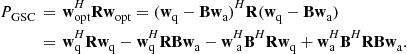 (12.67)
The unconstrained minimization of (12.67) results in the following expression for the adaptive component of the GSC:
![]() (12.68)
(12.68)
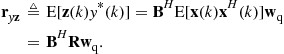
Noting that
![]() (12.69)
(12.69)
the following covariance matrix of the data vector ![]() and the correlation vector between
and the correlation vector between ![]() and
and ![]() can be introduced:
can be introduced:
![]() (12.70)
(12.70)
 (12.71)
Using the notations (12.70) and (12.71), the expression (12.68) can be finally written as
![]() (12.72)
(12.72)
which is again the Wiener-Hopf equation for finding optimal ![]() of a shorter length than
of a shorter length than ![]() .
.
The remaining question is how to choice the blocking matrix ![]() , if it is different from the projection matrix
, if it is different from the projection matrix ![]() . The blocking matrix
. The blocking matrix ![]() must satisfy the condition (12.66). In addition, it is desired that the dimension of the data vector at the output of
must satisfy the condition (12.66). In addition, it is desired that the dimension of the data vector at the output of ![]() , i.e., the dimension of the vector
, i.e., the dimension of the vector ![]() , be smaller than the dimension of the data vector
, be smaller than the dimension of the data vector ![]() . Thus, the matrix
. Thus, the matrix ![]() should be composed by linearly independent vectors
should be composed by linearly independent vectors ![]() so that
so that ![]() and the condition (12.66) becomes
and the condition (12.66) becomes
![]() (12.73)
(12.73)
where ![]() is the kth column of the matrix
is the kth column of the matrix ![]() .
.
There are many possible choices of ![]() . For example, for the GSC shown in Figure 12.15, the matrix
. For example, for the GSC shown in Figure 12.15, the matrix ![]() becomes a vector
becomes a vector
![]() (12.74)
(12.74)
while the blocking matrix ![]() is of the form
is of the form
 (12.75)
The corresponding vectors ![]() and
and ![]() are
are
![]() (12.76)
(12.76)
![]() (12.77)
(12.77)
and the vector ![]() has a shorter length then the vector
has a shorter length then the vector ![]() by one element.
by one element.
3.12.4.5 Correlated (coherent) SOI and interferences: spatial smoothing
Correlation between the SOI and interferences can occur, for example, because of signal multipath propagation (this effect is shown in Figure 12.16) or because of “smart” jammers [49]. The correlation between the SOI and interferences leads to a strong signal cancellation effect. It is because the optimal beamforming vector is obtained by minimizing the array output power subject to the SOI distortionless response constraint. If an interference is correlated (coherent) with the SOI, the minimum will be achieved if the array gain toward the interference is such that the interfering source exactly cancels the SOI. The distortionless response constraint is of no help in such a situation, since the array output does not have already the SOI component. As a result, robust techniques which would specifically address the situation of such correlation have been developed [49,50].

Figure 12.16 Correlated (coherent) signal and interferences occurring because of multipath propagation.
The following example visualizes the destructive effect of coherence (when the SOI and interference are correlated with the correlation coefficient 1). A ULA with ![]() omni-directional sensors spaced half-wavelength apart from each other is assumed. The DOA of a single SOI is
omni-directional sensors spaced half-wavelength apart from each other is assumed. The DOA of a single SOI is ![]() and
and ![]() dB, while the DOA of a single interference is
dB, while the DOA of a single interference is ![]() and
and ![]() dB. Figure 12.17 depicts the beampattern of the SMI adaptive beamformer for two cases of no correlation between the SOI and interference and full coherence between the SOI and interference. It can be seen that in the incoherent case, the directional pattern of the SMI beamformer has perfect mainlobe, low sidelobes and a deep null in the direction of the interference. However, in the coherent case, the directional pattern is completely destroyed.
dB. Figure 12.17 depicts the beampattern of the SMI adaptive beamformer for two cases of no correlation between the SOI and interference and full coherence between the SOI and interference. It can be seen that in the incoherent case, the directional pattern of the SMI beamformer has perfect mainlobe, low sidelobes and a deep null in the direction of the interference. However, in the coherent case, the directional pattern is completely destroyed.

The main idea of adaptive beamforming techniques robust against the SOI and interferences correlation is a decorrelation of the SOI and interferences by the means of electronic subaperture motion. Such technique is called spatial smoothing and it is demonstrated in Figure 12.18. On the left, the antenna array partitioned into subarrays is shown, while on the right, the blocks of the data covariance matrix that correspond to different subarrays are singled out.
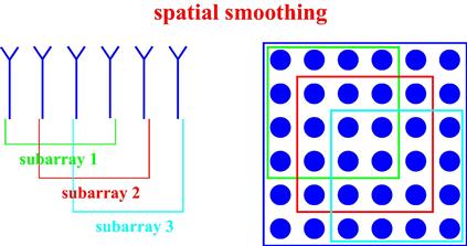
Figure 12.18 Decorrelation of the desired signal and interference by the means of electronic subaperture motion. The array consists of 6 sensors which form 3 subarrays of 4 sensors (on the left). A block of the data covariance matrix corresponds to each subarray (on the right). There are 3 covariance matrices for 3 subarrays.
Recall that the snapshot model is
 (12.78)
where ![]() is the vector of the waveforms of the SOI and the interferences.
is the vector of the waveforms of the SOI and the interferences.
According to Figure 12.18, the data vector in the pth subarray is
![]() (12.79)
(12.79)
where ![]() has a reduced dimension relative to
has a reduced dimension relative to ![]() and for the ULA configuration
and for the ULA configuration
![]() (12.80)
(12.80)
is a diagonal matrix, where ![]() are the DOA’s of the SOI and L interferences and d is the distance between any two adjacent antenna elements in ULA.
are the DOA’s of the SOI and L interferences and d is the distance between any two adjacent antenna elements in ULA.
Let the number of subarrays be
![]() (12.81)
(12.81)
where J is the subarray dimension, i.e., the number of antenna elements in one subarray. Then the ![]() spatially smoothed covariance matrix can be determined as
spatially smoothed covariance matrix can be determined as
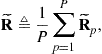 (12.82)
where
![]() (12.83)
(12.83)
is the covariance matrix for the pth subarray.
Substituting (12.79) in (12.83) and then substituting the result in (12.82), we obtain that
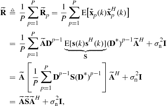 (12.84)
where the new notation
 (12.85)
is introduced.
Coherence between the SOI and interferences leads to a singular source covariance matrix ![]() . It is straightforward to see from (12.85) that even in the case of singular
. It is straightforward to see from (12.85) that even in the case of singular ![]() , the matrix
, the matrix ![]() becomes nonsingular if the number of subarrays is greater then the number of sources, that is,
becomes nonsingular if the number of subarrays is greater then the number of sources, that is,
![]() (12.86)
(12.86)
The decorrelation factor between sources i and l due to spatial smoothing can also be found and it is expressed as [51]
![]() (12.87)
(12.87)
Then the ![]() th elements of the matrices
th elements of the matrices ![]() and
and ![]() are given, respectively, as
are given, respectively, as
![]() (12.88)
(12.88)
where ![]() and
and ![]() are the variances of ith and lth sources, respectively, and
are the variances of ith and lth sources, respectively, and ![]() is the correlation coefficient between the ith and lth sources.
is the correlation coefficient between the ith and lth sources.
3.12.4.6 Forward-backward averaging and spatial smoothing
The spatial smoothing source decorrelation method, however, severely reduces the antenna array length because the number of subarrays must be larger than the number of correlated sources according to (12.81). Moreover, the spatial smoothing method does not exploit the structure of ULA or, in general, any array with centro-symmetric geometry, in a full measure. The antenna array length can be enlarged by the means of the so-called forward-backward ![]() FB
FB![]() spatial smoothing [52]. It is based on the observation that for any array with centro-symmetric geometry, we have
spatial smoothing [52]. It is based on the observation that for any array with centro-symmetric geometry, we have
 (12.89)
where ![]() is the exchange matrix.
is the exchange matrix.
In application to the covariance matrix for uncorrelated sources, the observation (12.89) leads to the following interesting result:
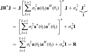 (12.90)
that is, the covariance matrix ![]() is the so-called centro-Hermitian matrix, satisfying
is the so-called centro-Hermitian matrix, satisfying ![]() .
.
Using (12.90), the idea of the FB averaging is to decorrelate the coherent/correlated sources by the means of enforcing the centro-Hermitian property, i.e., by computing the following FB covariance matrix:
![]() (12.91)
(12.91)
Combining the FB averaging with spatial smoothing, it is possible to double the number of subarrays while keeping the subarray length the same as in the conventional spatial smoothing. Then the covariance matrix for the FB spatial smoothing is defined as
 (12.92)
As a result, the same decorrelation factor can be archived by the FB spatial smoothing with the use of subarrays of a bigger size as the one achieved by the conventional spatial smoothing with subarrays of a smaller size.
The FB spatial smoothing method can be further generalized by introducing the weights ![]()
![]() as follows
as follows
 (12.93)
and optimizing these weights to minimize the source decorrelation factor further.
One more simple source decorrelation method, named redundancy averaging [53], is based on the fact that the true data covariance matrix in a ULA must be a Toeplitz matrix. The sample estimate of the data covarince matrix is in general not a Toeplitz matrix. However, the Toeplitz structure can be enforced, for example, by averaging the diagonals of the sample covariance matrix as it is shown in Figure 12.19. In addition to enforcing the Toeplitz structure, such redundancy averaging also leads to source decorrelation.

3.12.4.7 Rapidly moving interferences
If the rate/vilosity of interference motion is faster than the rate of adaptation of the adaptive array, the antenna array may be unable to follow such rapid changes of the interference position. The situation of fast moving interference is, however, common in a large number of applications [19]. An example of such situation is shown in Figure 12.20. The nulls of the beampattern are very narrow and even relatively slow interference motion may lead to the situation when the interference leaks to the output of adaptive beamformer through a sidelobe that may significantly reduce the output SINR of adaptive beamformer.

The situation of rapidly moving interferences is typically addressed in terms of broadening the adaptive pattern nulls towards the interfering sources. The main difficulty here is that the DOAs of interfering sources are unknown. However, the null width even towards interfering sources with unknown DOAs can be increased by replacing the sample covariance matrix with the modified covariance matrix of the form [19,54]
![]() (12.94)
(12.94)
where ![]() stands for element-wise Hadamard product of matrices and the matrix
stands for element-wise Hadamard product of matrices and the matrix ![]() is a positive semi-definite matrix that is called a taper matrix. The choice of tapper is not unique. In the most popular tapper proposed in [54], the
is a positive semi-definite matrix that is called a taper matrix. The choice of tapper is not unique. In the most popular tapper proposed in [54], the ![]() th element of the taper matrix
th element of the taper matrix ![]() is given by
is given by
![]() (12.95)
(12.95)
where ![]() defines the required null width.
defines the required null width.
Broadening the adaptive pattern nulls can also be archived by the means of enforcing the so-called data-dependent derivative constraints [55]. The resulting covariance matrix takes the form
![]() (12.96)
(12.96)
where ![]() is the known diagonal matrix of sensor coordinates and the parameter
is the known diagonal matrix of sensor coordinates and the parameter ![]() defines the tradeoff between null depth and width. It has been shown that the null broadening method based on (12.96) can be also interpreted in terms of the covariance tapering method of (12.94) (see [55]).
defines the tradeoff between null depth and width. It has been shown that the null broadening method based on (12.96) can be also interpreted in terms of the covariance tapering method of (12.94) (see [55]).
3.12.4.8 Unified principle to MVDR robust adaptive beamforming design
As we have seen earlier, the SMI beamformer is not robust to an imperfect knowledge of the SOI steering vector. Different robust adaptive beamforming techniques which use different specific notions of robustness such as robustness against small sample size, pointing error, coherence between the SOI and interferences, and rapid interference motion have been revised. Each of these notions of robustness is very specific. For example, the point or derivative mainbeam constraint-based beamforming technique is very useful for overcoming pointing error problem, but it does not help in the general case of mismatched SOI wavefront and finite sample size when the SOI is present in the antenna array measurements.
The general meaning of robustness for any robust adaptive beamforming technique can be, however, defined as the ability of such technique to compute the beamforming vector so that the SINR is maximized despite possibly imperfect and incomplete knowledge of required prior information. More specifically, the aforementioned signal cancellation effect for the SMI beamformer occurs in the situation when the SOI steering vector is misinterpreted with any of the interference steering vectors of their linear combinations. Thus, if with incomplete and/or imperfect prior information, a robust adaptive beamforming technique is able to estimate the SOI steering vector so that the estimate does not converge to any of the interferences and their linear combinations, such technique is called robust. Using this notion of robustness, the unified principle to robust adaptive beamforming design based on MVDR beamformer can be formulated as follows. Use the standard SMI beamformer (12.36) in tandem with SOI steering vector estimation performed based on some possibly incomplete and inaccurate prior information. The difference between different MVDR robust adaptive beamforming techniques can be then shown to boil down to the differences in the assumed prior information, the specific notions of robustness, and the corresponding steering vector estimation techniques used.
Hereafter, the imperfectly known presumed SOI steering vector is denoted as ![]() , while
, while ![]() stands for the actual SOI steering vector that is different from
stands for the actual SOI steering vector that is different from ![]() , i.e.,
, i.e., ![]() . The estimate of the actual SOI steering vector is denoted as
. The estimate of the actual SOI steering vector is denoted as ![]() . In the techniques that follow, the estimate
. In the techniques that follow, the estimate ![]() is found by using different prior information and based on different principles. Other than that, all the techniques are based on the aforementioned unified principle.
is found by using different prior information and based on different principles. Other than that, all the techniques are based on the aforementioned unified principle.
Many modern robust adaptive beamforming techniques are based on convex optimization theory [16,56,57]. Most of such robust beamformers cannot be expressed in closed-form, i.e., cannot be written in terms of the covariance matrix inversion or eigenvalue decomposition. However, the complexity of solving optimization problems that correspond to such beamforming techniques is comparable to the complexity of matrix inversion. Thus, there is no significant difference in terms of computational complexity between the so-called closed-form solutions and numerical solutions of convex problems.
3.12.4.9 Eigenspace-based beamformer
Using the a priori knowledge of the presumed SOI steering vector ![]() , the eigenspace-based beamformer computes and uses the projection of
, the eigenspace-based beamformer computes and uses the projection of ![]() onto the sample signal-plus-interference subspace as a corrected estimate of the actual SOI steering vector. The eigendecomposition of (12.5) yields
onto the sample signal-plus-interference subspace as a corrected estimate of the actual SOI steering vector. The eigendecomposition of (12.5) yields
![]() (12.97)
(12.97)
where the ![]() matrix
matrix ![]() and
and ![]() matrix
matrix ![]() contain the signal-plus-interference subspace eigenvectors of
contain the signal-plus-interference subspace eigenvectors of ![]() and the noise subspace eigenvectors, respectively, while the
and the noise subspace eigenvectors, respectively, while the ![]() matrix
matrix ![]() and
and ![]() matrix
matrix ![]() contain the eigenvalues corresponding to
contain the eigenvalues corresponding to ![]() and
and ![]() , respectively, and as before L stands for the number of interfering signals.
, respectively, and as before L stands for the number of interfering signals.
The estimate of the actual SOI steering vector is found as
![]() (12.98)
(12.98)
where ![]() is the projection matrix to the desired signal-plus-interference subspace. Then the eigenspace-based beamformer is obtained by substituting the so-obtained estimate of the steering vector to the SMI beamformer (12.36), and it can be expressed as [58]
is the projection matrix to the desired signal-plus-interference subspace. Then the eigenspace-based beamformer is obtained by substituting the so-obtained estimate of the steering vector to the SMI beamformer (12.36), and it can be expressed as [58]
![]() (12.99)
(12.99)
where the fact that
![]() (12.100)
(12.100)
has been used for obtaining the last equality and ![]() because
because ![]() and
and ![]() are orthogonal (see the decomposition (12.97)).
are orthogonal (see the decomposition (12.97)).
Summarizing, the essence of the eigenspace-based beamforming technique is to project the presumed SOI steering vector onto the measured signal-plus-interference subspace prior to processing in order to reduce the signal wavefront mismatch. Then, the estimate of the actual SOI steering vector is plugged to the standard SMI beamformer. The interference rejection part remains unchanged for this beamformer as compared to the SMI beamformer. The prior information used is the presumed steering vector ![]() and the number of interfering sources L. The notion of robustness is the projection of the presumed steering vector to the signal-plus-interference subspace. It is, however, well known that at low SNR, the eigenspace-based beamformer suffers from a high probability of subspace swap and incorrect estimation of the signal-plus-interference subspace dimension [59].
and the number of interfering sources L. The notion of robustness is the projection of the presumed steering vector to the signal-plus-interference subspace. It is, however, well known that at low SNR, the eigenspace-based beamformer suffers from a high probability of subspace swap and incorrect estimation of the signal-plus-interference subspace dimension [59].
3.12.4.10 Worst-case-based robust adaptive beamforming
This approach is based on explicitly modeling of the actual SOI steering vector ![]() as a sum of the presumed steering vector and a deterministic norm bounded mismatch vector
as a sum of the presumed steering vector and a deterministic norm bounded mismatch vector ![]() , that is,
, that is,
![]() (12.101)
(12.101)
where ![]() is some a priori known bound. Thus, the worst-case-based robust adaptive beamformer uses the prior information about the presumed steering vector and the information that the mismatch vector is norm bounded [60]. An ellipsoidal uncertainty region can also be considered instead of the mentioned in (12.101) spherical uncertainty [61]. However, a more sophisticated prior information has to be available in the case of ellipsoidal uncertainty. Assuming spherical uncertainty for
is some a priori known bound. Thus, the worst-case-based robust adaptive beamformer uses the prior information about the presumed steering vector and the information that the mismatch vector is norm bounded [60]. An ellipsoidal uncertainty region can also be considered instead of the mentioned in (12.101) spherical uncertainty [61]. However, a more sophisticated prior information has to be available in the case of ellipsoidal uncertainty. Assuming spherical uncertainty for ![]() , i.e., introducing the uncertainty set
, i.e., introducing the uncertainty set
![]() (12.102)
(12.102)
the worst-case-based robust adaptive beamforming aims at solving the following optimization problem [60]
![]() (12.103)
(12.103)
The optimization problem (12.103) is equivalent to the following second-order cone (SOC) programming problem [60]
![]() (12.104)
(12.104)
which can be solved efficiently using standard numerical optimization methods with complexity comparable to the complexity of matrix inversion.
The worst-case-based robust adaptive beamforming technique (12.103) can be equivalently interpreted as the standard SMI beamformer used in tandem with the SOI steering vector estimate obtained by solving the following covariance fitting problem [62]
![]() (12.105)
(12.105)
Summarizing, the prior information used in the worst-case-based robust adaptive beamforming techniques is the presumed steering vector and the value ![]() , which may be difficult to obtain in practice. The notion of robustness is the uncertainty region for the presumed steering vector. The robustness to the rapidly moving interference sources can also be added to the worst-case-based robust adaptive beamforming [63].
, which may be difficult to obtain in practice. The notion of robustness is the uncertainty region for the presumed steering vector. The robustness to the rapidly moving interference sources can also be added to the worst-case-based robust adaptive beamforming [63].
3.12.4.11 Relationship between the worst-case-based and the LSMI adaptive beamformers
Note that the constraint in the optimization problem (12.103) must be satisfied with equality at optimality. Indeed, if the constraint is not satisfied with equality, then the minimum of the objective function in (12.103) is achieved when ![]() . However, by replacing
. However, by replacing ![]() with
with ![]() , the objective function of (12.103) can be decreased by the factor of
, the objective function of (12.103) can be decreased by the factor of ![]() , whereas the constraint in (12.103) will be still satisfied. This contradicts the original statement that the objective function is minimized when
, whereas the constraint in (12.103) will be still satisfied. This contradicts the original statement that the objective function is minimized when ![]() . Therefore, the minimum of the objective function is achieved at
. Therefore, the minimum of the objective function is achieved at ![]() , and the inequality constraint in (12.103) is equivalent to the equality constraint. This also means that
, and the inequality constraint in (12.103) is equivalent to the equality constraint. This also means that ![]() is real-valued and positive. Using these facts, the problem (12.103) can be rewritten as
is real-valued and positive. Using these facts, the problem (12.103) can be rewritten as
![]() (12.106)
(12.106)
The solution to (12.106) can be found by using the method Lagrange multipliers, i.e., by optimizing the following Lagrangian:
![]() (12.107)
(12.107)
where ![]() is a Lagrange multiplier. Taking the gradient of (12.107) and equating it to zero, it can be found that
is a Lagrange multiplier. Taking the gradient of (12.107) and equating it to zero, it can be found that
![]() (12.108)
(12.108)
Furthermore, applying the matrix inversion lemma to (12.108), the beamforming vector can be expressed as [60]
![]() (12.109)
(12.109)
which is the LSMI beamformer with adaptive diagonal loading factor. The expression (12.109) cannot be used practically since the optimal value of ![]() has to be first found. The numerical algorithms designed in [61] are particularly based on finding
has to be first found. The numerical algorithms designed in [61] are particularly based on finding ![]() numerically, while the general SOC programming is used in [60]. The complexity of both type of methods is, however, the same and is comparable to the matrix inversion as in SMI and LSMI beamformers.
numerically, while the general SOC programming is used in [60]. The complexity of both type of methods is, however, the same and is comparable to the matrix inversion as in SMI and LSMI beamformers.
3.12.4.12 Doubly constrained robust adaptive beamforming
The doubly constrained robust adaptive beamforming [64] is similar to the worst-case-based one (12.103) (equivalently (12.105)), but it exposes also an additional constraint to the norm of the steering vector estimate, that is, ![]() . Then the corresponding optimization problem for finding
. Then the corresponding optimization problem for finding ![]() is
is
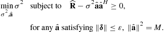 (12.110)
This method uses the same prior information as the worst-case-based robust adaptive beamforming method and obviously fits under the aforementioned unified framework. Although the spherical uncertainty region is considered in [64], it can be relatively straightforwardly extended to the ellipsoidal uncertainty region [65]. Clearly, the notion of robustness for this method is the same as for the worst-case-based one. Due to the constraint ![]() , the doubly constrained robust adaptive beamforming provides a better estimate of the SOI than the worst-case-based robust adaptive beamforming. It can be important in the applications where such estimate is needed.
, the doubly constrained robust adaptive beamforming provides a better estimate of the SOI than the worst-case-based robust adaptive beamforming. It can be important in the applications where such estimate is needed.
3.12.4.13 Probabilistically constrained robust adaptive beamforming
Another approach to robust adaptive beamforming is based on the assumption that the mismatch vector ![]() is random. Then the problem has to be formulated in probabilistic terms in contrast to the deterministic terms used in the worst-case-based design. Specifically, the probabilistically constrained robust adaptive beamforming problem is formulated as [66]
is random. Then the problem has to be formulated in probabilistic terms in contrast to the deterministic terms used in the worst-case-based design. Specifically, the probabilistically constrained robust adaptive beamforming problem is formulated as [66]
![]() (12.111)
(12.111)
where ![]() denotes probability and
denotes probability and ![]() is preselected probability value. In this case, the prior information is the presumed steering vector
is preselected probability value. In this case, the prior information is the presumed steering vector ![]() as before, but since the steering vector mismatch is assumed to be random, the other prior information is the distribution type and the distribution variance of
as before, but since the steering vector mismatch is assumed to be random, the other prior information is the distribution type and the distribution variance of ![]() as well as the non-outage probability
as well as the non-outage probability ![]() for the distortionless response constraint. In two cases when
for the distortionless response constraint. In two cases when ![]() is Gaussian distributed and the distribution of
is Gaussian distributed and the distribution of ![]() is unknown and assumed to be the worst possible, it has been shown that the problem (12.111) can be closely approximated by the following problem [66]:
is unknown and assumed to be the worst possible, it has been shown that the problem (12.111) can be closely approximated by the following problem [66]:
![]() (12.112)
(12.112)
where ![]() is the covariance matrix of the random mismatch vector
is the covariance matrix of the random mismatch vector ![]() and
and ![]() if
if ![]() is Gaussian distributed and
is Gaussian distributed and ![]() if the distribution of
if the distribution of ![]() is unknown. Thus, the latter problem boils down mathematically to the same form as the worst-case-based robust adaptive beamforming problem and can also be considered as a part of the earlier explained unified framework. However, the prior information required for the probabilistically constrained robust adaptive beamforming may be easier to obtain than that for the worst-case-based approach since it is typically easier to estimate the statistics of the mismatch distribution reliably, while
is unknown. Thus, the latter problem boils down mathematically to the same form as the worst-case-based robust adaptive beamforming problem and can also be considered as a part of the earlier explained unified framework. However, the prior information required for the probabilistically constrained robust adaptive beamforming may be easier to obtain than that for the worst-case-based approach since it is typically easier to estimate the statistics of the mismatch distribution reliably, while ![]() has a clear physical meaning. The non-outage probability
has a clear physical meaning. The non-outage probability ![]() for the distortionless response constraint is the specific notion of robustness used in this approach.
for the distortionless response constraint is the specific notion of robustness used in this approach.
3.12.4.14 Sequential quadratic programming-based robust adaptive beamforming
The title of this approach refers to the optimization technique used, but its essence is significantly different from the above approaches that are based on the same aforementioned unified principle to robust MVDR beamforming design. According to this approach the estimate of the actual steering vector ![]() is found so that the beamformer output power is maximized while the convergence of the estimate
is found so that the beamformer output power is maximized while the convergence of the estimate ![]() to any interference steering vector is prohibited [67]. The rationale behind maximization of the beamformer output power is the following. In the steering vector mismatched case, the solution (12.36) can be re-written as a function of unknown
to any interference steering vector is prohibited [67]. The rationale behind maximization of the beamformer output power is the following. In the steering vector mismatched case, the solution (12.36) can be re-written as a function of unknown ![]() , that is,
, that is, ![]() . Using
. Using ![]() , the beamformer output power can be also written as a function of the mismatch
, the beamformer output power can be also written as a function of the mismatch ![]() as
as
![]() (12.113)
(12.113)
Thus, the estimate of ![]() or, equivalently, the estimate of
or, equivalently, the estimate of ![]() that maximizes (12.113) will be the best estimate of the actual steering vector
that maximizes (12.113) will be the best estimate of the actual steering vector ![]() under the constraints that the norm of
under the constraints that the norm of ![]() equals
equals ![]() and
and ![]() does not converge to any of the interference steering vectors. The latter is guaranteed in this method by requiring that
does not converge to any of the interference steering vectors. The latter is guaranteed in this method by requiring that
![]() (12.114)
(12.114)
where ![]() are the T dominant eigenvectors of the matrix
are the T dominant eigenvectors of the matrix ![]() is the steering vector associated with direction
is the steering vector associated with direction ![]() and having the structure defined by the antenna geometry,
and having the structure defined by the antenna geometry, ![]() is the angular sector in which the SOI is located,
is the angular sector in which the SOI is located, ![]() and
and ![]() stand for the estimates of the steering vector mismatch and the actual SOI steering vector, respectively. The optimization problem for finding the estimate
stand for the estimates of the steering vector mismatch and the actual SOI steering vector, respectively. The optimization problem for finding the estimate ![]() can be written as [67]
can be written as [67]
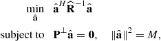 (12.115)
![]()
where ![]() and the sector
and the sector ![]() is the complement of the sector
is the complement of the sector ![]() . The last constraint in (12.115) limits the noise power collected in
. The last constraint in (12.115) limits the noise power collected in ![]() .
.
Since the optimization problem (12.115) is non-convex and difficult to solve, it is modified so that the orthogonal component of ![]() (here
(here ![]() is decomposed to colinear and orthogonal components) is estimated iteratively as shown in Figure 12.21, while at each iteration the following quadratic (convex) optimization problem is solved
is decomposed to colinear and orthogonal components) is estimated iteratively as shown in Figure 12.21, while at each iteration the following quadratic (convex) optimization problem is solved
 (12.116)
![]()
where ![]() is the component of
is the component of ![]() that is orthogonal to
that is orthogonal to ![]() and the orthogonality between
and the orthogonality between ![]() and
and ![]() is imposed by adding the constraint
is imposed by adding the constraint ![]() . Because the quadratic programming problem (12.116) has to be solved sequentially, the corresponding method is called the sequential quadratic programming (SQP)-based robust adaptive beamforming.
. Because the quadratic programming problem (12.116) has to be solved sequentially, the corresponding method is called the sequential quadratic programming (SQP)-based robust adaptive beamforming.

It can be seen that the prior information used in this approach is the presumed steering vector and the angular sector ![]() in which the desired signal is located. Note that if the constraint (12.114) is replaced by the constraint
in which the desired signal is located. Note that if the constraint (12.114) is replaced by the constraint ![]() , the convergence to an interference steering vector is also be avoided, but the problem then becomes equivalent to the worst-case-based robust adaptive beamforming (see [64]). This technique can be simplified for more structured uncertainties, for example, when it is known that the array is partially calibrated [68]. However, the amount of required prior information about the uncertainty then increases.
, the convergence to an interference steering vector is also be avoided, but the problem then becomes equivalent to the worst-case-based robust adaptive beamforming (see [64]). This technique can be simplified for more structured uncertainties, for example, when it is known that the array is partially calibrated [68]. However, the amount of required prior information about the uncertainty then increases.
3.12.4.15 Eigenvalue beamforming using multi-rank MVDR beamformer
If the desired signal and interference steering vectors lie in known signal subspaces and the rank of the signal correlation matrix is known, the eigenvalue beamforming using multi-rank MVDR beamformer can be efficient [69]. The multi-rank beamformer matrix is computed as
![]() (12.117)
(12.117)
where ![]() is a data dependent left-orthogonal matrix, i.e.,
is a data dependent left-orthogonal matrix, i.e., ![]() , and
, and ![]() is the matrix with the columns that span the linear subspace in which the SOI lies. For example, for resolving a signal with a rank-one covariance matrix and an unknown but fixed DOA, the columns of
is the matrix with the columns that span the linear subspace in which the SOI lies. For example, for resolving a signal with a rank-one covariance matrix and an unknown but fixed DOA, the columns of ![]() should be selected as the dominant eigenvectors of the mismatch covariance matrix, i.e.,
should be selected as the dominant eigenvectors of the mismatch covariance matrix, i.e.,
![]() (12.118)
(12.118)
If it is assumed that the signal lies in a known subspace, but the DOA is unknown and unfixed (randomly changes from snapshot to snapshot), it is the subdominant eigenvectors of the mismatch covariance matrix that should be used as the columns of the matrix ![]() .
.
The prior information required for this beamforming technique is the linear subspace in which the desired signal lies and the rank of the desired signal covariance matrix. The main disadvantages are that a very specific modeling of the covariance matrix is used and the signal subspace has to be known.
3.12.4.16 Robust adaptive beamforming based on steering vector estimation with as little as possible prior information
The essence of robustness can be practically viewed as an ability of adaptive beamformer to achieve acceptably high output SINR despite imprecise and perhaps very limited prior information. This beamforming technique aims at fulfilling such most general notion of robustness. Assume that the SOI lies in the known angular sector ![]() that is distinguishable from general locations of the interfering signals. The estimate
that is distinguishable from general locations of the interfering signals. The estimate ![]() can be forced not to converge to any vector with DOAs within the complement of
can be forced not to converge to any vector with DOAs within the complement of ![]() including the interference steering vectors and their linear combinations by the means of the following constraint [70,71]:
including the interference steering vectors and their linear combinations by the means of the following constraint [70,71]:
![]() (12.119)
(12.119)
where ![]() is a uniquely selected value for a given angular sector
is a uniquely selected value for a given angular sector ![]() , that is,
, that is,
![]() (12.120)
(12.120)
It is worth stressing that no restrictions/assumptions on the structure of the interferences are needed. Moreover, the interferences do not need to have the same structure as the SOI.
In order to illustrate how the quadratic constraint (12.119) works, let us consider the following example. Consider ULA of 10 omni-directional antenna elements spaced half wavelength apart from each other. Let the range of the SOI angular locations be ![]() . Figure 12.22 depicts the values of the quadratic term
. Figure 12.22 depicts the values of the quadratic term ![]() for different angles. The rectangular bar in the figure marks the directions within the angular sector
for different angles. The rectangular bar in the figure marks the directions within the angular sector ![]() . It can be observed from this figure that the term
. It can be observed from this figure that the term ![]() takes the smallest values within the angular sector
takes the smallest values within the angular sector ![]() and increases outside of the sector. Therefore, if
and increases outside of the sector. Therefore, if ![]() is selected to be equal to the maximum value of the term
is selected to be equal to the maximum value of the term ![]() within the angular sector
within the angular sector ![]() , the constraint (12.119) guarantees that the estimate of the desired signal steering vector does not converge to any of the interference steering vectors and their linear combinations. The equality
, the constraint (12.119) guarantees that the estimate of the desired signal steering vector does not converge to any of the interference steering vectors and their linear combinations. The equality ![]() must occur at one of the edges of
must occur at one of the edges of ![]() . However, the value of the quadratic term might be smaller than
. However, the value of the quadratic term might be smaller than ![]() at the other edge of
at the other edge of ![]() . Therefore, a possibly larger sector
. Therefore, a possibly larger sector ![]() has to be defined, at which the equality
has to be defined, at which the equality ![]() holds at both edges.
holds at both edges.
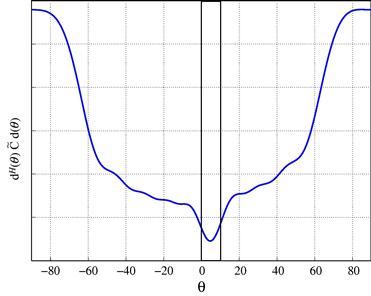
Figure 12.22 Values of the term ![]() in the constraint (12.119) for different angles.
in the constraint (12.119) for different angles.
Although for computing the matrix ![]() , the presumed knowledge of the antenna array geometry is used, an inaccurate information about the antenna array geometry is sufficient. It further stresses on the robustness of such beamforming design to the imperfect prior information [71]. Taking into account the normalization constraint and the constraint (12.119), the problem of estimating the SOI steering vector based on the knowledge of the sector
, the presumed knowledge of the antenna array geometry is used, an inaccurate information about the antenna array geometry is sufficient. It further stresses on the robustness of such beamforming design to the imperfect prior information [71]. Taking into account the normalization constraint and the constraint (12.119), the problem of estimating the SOI steering vector based on the knowledge of the sector ![]() can be formulated as the following optimization problem:
can be formulated as the following optimization problem:
 (12.121)
![]()
Compared to the other MVDR robust adaptive beamforming methods, which require the knowledge of the presumed steering vector and, thus, the knowledge of the presumed antenna array geometry and propagation media and source characteristics, only imprecise knowledge of the antenna array geometry and approximate knowledge of the angular sector ![]() are needed for the robust adaptive beamformer (12.121).
are needed for the robust adaptive beamformer (12.121).
As cooperated to the SQP-based beamformer (12.116), where the constraint ![]() enforces the estimated steering vector to be a linear combination of T dominant eigenvectors
enforces the estimated steering vector to be a linear combination of T dominant eigenvectors ![]() , the steering vector in (12.121) is not restricted by such linear combination requirement, while the convergence to any of the interference steering vectors and their linear combinations is avoided by the means of the constraint (12.119). As a result, the beamformer (12.121) has more degrees of freedom compared to the SQP-based beamformer. Thus, it is expected that it outperform the latter one. Finally, due to the non-convex equality constraint, the problem (12.121) is non-convex and NP-hard in general. The efficient polynomial-time solution to this problem is developed in [71] based on the semi-definite programming relaxation theory [57,72,73].
, the steering vector in (12.121) is not restricted by such linear combination requirement, while the convergence to any of the interference steering vectors and their linear combinations is avoided by the means of the constraint (12.119). As a result, the beamformer (12.121) has more degrees of freedom compared to the SQP-based beamformer. Thus, it is expected that it outperform the latter one. Finally, due to the non-convex equality constraint, the problem (12.121) is non-convex and NP-hard in general. The efficient polynomial-time solution to this problem is developed in [71] based on the semi-definite programming relaxation theory [57,72,73].
3.12.4.17 Comparison by simulation
To compare a number of aforementioned MVDR robust adaptive beamforming methods based on the unified approach, the following example is considered. A ULA of 10 omni-directional sensors with the inter-element spacing of half wavelength is used. Additive noise in antenna elements is modeled as spatially and temporally independent complex Gaussian noise with zero mean and unit variance. Two interfering sources are assumed to impinge on the antenna array from the directions ![]() and
and ![]() , while the presumed direction towards the SOI is assumed to be
, while the presumed direction towards the SOI is assumed to be ![]() . The INR equals 30 dB and the desired signal is always present in the training data.
. The INR equals 30 dB and the desired signal is always present in the training data.
The robust adaptive beamforming (12.121) is compared with the eigenspace-based, the worst-case-based, the SQP-based, and the LSMI robust adaptive beamforming techniques. For the beamformer (12.121) and the SQP-based one, the angular sector of interest ![]() is assumed to be
is assumed to be ![]() , where
, where ![]() is the presumed DOA of the SOI. The difference between the presumed and actual positions of each antenna element is modeled as a uniform random variable distributed in the interval
is the presumed DOA of the SOI. The difference between the presumed and actual positions of each antenna element is modeled as a uniform random variable distributed in the interval ![]() measured in wavelength. In addition to the antenna element displacements, the signal steering vector is distorted by wave propagation effects in an inhomogeneous medium. Independent-increment phase distortions are accumulated by the components of the presumed steering vector. It is assumed that the phase increments remain fixed in each simulation run.
measured in wavelength. In addition to the antenna element displacements, the signal steering vector is distorted by wave propagation effects in an inhomogeneous medium. Independent-increment phase distortions are accumulated by the components of the presumed steering vector. It is assumed that the phase increments remain fixed in each simulation run.
Figure 12.23 depict the output SINR performance of the aforementioned robust adaptive beamforming techniques tested versus the SNR for fixed training data size ![]() . As it can be observed from the figures, the beamformer (12.121) has a better performance even if there is an error in the knowledge of the antenna array geometry.
. As it can be observed from the figures, the beamformer (12.121) has a better performance even if there is an error in the knowledge of the antenna array geometry.

3.12.4.18 Robust adaptive beamforming for the general-rank signal model
Robust adaptive beamforming techniques for general-rank signal model address the situation when the desired signal covariance matrix ![]() is not known precisely as well as the sample estimate of the data covariance matrix (12.5) is inaccurate because of small sample size.
is not known precisely as well as the sample estimate of the data covariance matrix (12.5) is inaccurate because of small sample size.
In order to provide robustness against the norm-bounded mismatches ![]() and
and ![]() (where
(where ![]() and
and ![]() are some preselected bounds) in the SOI and data sample covariance matrices, respectively, the following worst-case-based robust adaptive beamformer has been derived [74,75]
are some preselected bounds) in the SOI and data sample covariance matrices, respectively, the following worst-case-based robust adaptive beamformer has been derived [74,75]
![]() (12.122)
(12.122)
Although it is a simple closed-form solution, it is overly conservative due to the fact that the negatively diagonally loaded signal covariance matrix ![]() can be indefinite. A less conservative robust adaptive beamforming problem formulation, which enforces the matrix
can be indefinite. A less conservative robust adaptive beamforming problem formulation, which enforces the matrix ![]() to be positive semi-definite has been considered in [76]. Defining
to be positive semi-definite has been considered in [76]. Defining ![]() , which is for example the Cholesky decomposition, the corresponding robust adaptive beamforming problem for a norm bounded-mismatch
, which is for example the Cholesky decomposition, the corresponding robust adaptive beamforming problem for a norm bounded-mismatch ![]() (where
(where ![]() is some value found based on the bound value
is some value found based on the bound value ![]() ) to the matrix
) to the matrix ![]() is given as [76]
is given as [76]
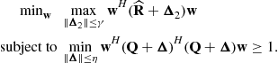 (12.123)
If the mismatch of the signal covariance matrix is small enough, the optimization problem (12.123) can be equivalently recast as
![]() (12.124)
(12.124)
Due to the non-convex (difference-of-convex functions (DC)) constraint, the problem (12.124) is non-convex. Although the DC programming problems are believed to be NP-hard in general, the problem (12.124) is shown to have very efficient polynomial-time solution [77].
3.12.4.19 Wideband robust adaptive beamforming
In the wideband case (see Figure 12.8), the SOI components at different frequencies are typically not perfectly phased-aligned by the presteering delays because of multiple practical imperfections. The reasons for imperfections are accentually the same as in the narrowband case with an addition of more error sources such as the presteering delay quantization effects. Therefore, there are errors that can be modeled in terms of the phase error vector ![]() that is the function of the frequency f. Then the actual components of the SOI arriving from DOA
that is the function of the frequency f. Then the actual components of the SOI arriving from DOA ![]() after the presteering delay filter are [78]
after the presteering delay filter are [78]
![]() (12.125)
(12.125)
instead of (12.13) in the case of no mismatch. Here ![]() is a common time delay at each of the M sensors and
is a common time delay at each of the M sensors and ![]() is the minimum frequency of the SOI.
is the minimum frequency of the SOI.
Defining the mismatch set that contains all possible phase error vectors at the frequency f as ![]() , the wideband robust adaptive beamforming problem can be written as
, the wideband robust adaptive beamforming problem can be written as
![]() (12.126)
(12.126)
Using (12.15) and (12.125), the array response towards DOA ![]() can be written as [78]
can be written as [78]
![]() (12.127)
(12.127)
where ![]() is
is ![]() matrix.
matrix.
Using the triangular and then Cauchy-Schwarz inequalities, the magnitude of the lower bound for the array responde (12.127) can be found as
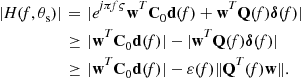 (12.128)
Finally, using the lower bound (12.128) for the constraint ![]() in (12.126) and imposing a linear phase constraint on each of the M FIR filters of the array processor Figure 12.8, the optimization problem (12.126) can be reformulated as the following output power minimization problem:
in (12.126) and imposing a linear phase constraint on each of the M FIR filters of the array processor Figure 12.8, the optimization problem (12.126) can be reformulated as the following output power minimization problem:
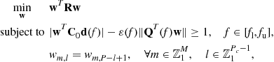 (12.129)
where ![]() is the covariance matrix of the stacked snapshot vectors,
is the covariance matrix of the stacked snapshot vectors, ![]() , and
, and ![]() denotes the ring of integers from i to j. The last constraint in the optimization problem (12.129) ensures the linear phase at each of the M FIR filters and it provides additional robustness against presteering errors [78]. The problem (12.129) is non-convex, but it can be reformulated to a convex problem that can be solved efficiently [78]. The disadvantage is, however, that the constraint on the magnitude of the array response is strengthened by using the triangular and Cauchy-Schwarz inequalities (see (12.128)). More sophisticated wideband robust adaptive beamforming designs can be also found in [79,80].
denotes the ring of integers from i to j. The last constraint in the optimization problem (12.129) ensures the linear phase at each of the M FIR filters and it provides additional robustness against presteering errors [78]. The problem (12.129) is non-convex, but it can be reformulated to a convex problem that can be solved efficiently [78]. The disadvantage is, however, that the constraint on the magnitude of the array response is strengthened by using the triangular and Cauchy-Schwarz inequalities (see (12.128)). More sophisticated wideband robust adaptive beamforming designs can be also found in [79,80].
3.12.4.20 Summary
The applicability of different robust adaptive beamforming techniques is mainly defined by the corresponding notions of robustness used for designing a particular method and by the required prior information needed to run a method. A majority of the existing robust adaptive beamforming techniques such as the above mentioned techniques as eigenspace-based, worst-case-based, doubly constrained, probabilistically constrained techniques as well as the eigenvalue beamforming using multi-rank MVDR beamformer and their various modifications require the knowledge of the presumed steering vector. In turn, the availability of this knowledge implies that the source and propagation media characteristics as well as antenna geometry are known with a certain accuracy. Each method also requires some additional information. For example, the eigenspace-based beamformer needs to know the number of interferences, which may be a challenging practical problem. The worst-case-based and the doubly constrained beamforming techniques need to know the upper-bound to the norm of the steering vector mismatch, which is fortunately irrelevant to specific causes of mismatch and which is practically easy to guess or estimate in a particular application. It is important that the performance of these methods is not very sensitive to the over- or under-estimation of upper-bound to the norm of the steering vector mismatch that makes these approaches practically attractive and widely applicable. The probabilistically constrained robust adaptive beamforming enables to quantify the upper-bound to the norm of the steering vector mismatch in terms of the variance of the steering vector estimation and the practically tolerable outage probability that the distortionless response constraint is satisfied. This may be an advantage in a number of applications especially when the variance of the steering vector/channel estimation is already the existing information that does not require any additional efforts to obtain. However, the least restrictive in terms of the required prior information is the robust adaptive beamforming technique based on steering vector estimation with as little as possible prior information. It does not need the information about the presumed steering vector, but only needs a very approximate knowledge of the array geometry, which is easy to have even in such challenging applications as sonar. Similarly, it does not need any nearly accurate estimates of the source characteristics, but rather needs only the very approximate knowledge of a sector where the source of interest is located. In this respect, the latter technique can be most appropriately called “robust.” Moreover, it outperforms other existing technique in terms of the beamformer output SINR. However, the complexity of the latter technique is equivalent to the complexity of solving SDP problem that may be higher than the complexity of matrix inversion, i.e., the complexity of SMI and LSMI beamformers, and nearly the complexity of the worst-case-based and other aforementioned beamforming techniques. Finally, the notion of robustness used by the robust adaptive beamforming technique based on steering vector estimation with as little as possible prior information is the most general that makes its applicability essentially unlimited (limited only by the source model as the source is assumed to be narrowband). The extension of this technique to the wideband case is the topic of future promising research.
The field of robust adaptive beamforming is an actively developing research field which is strongly connected to the progress in optimization theory. While the notion of robustness used in [71] is the most general as mentioned above, new methods have been actively developing within the other approaches to robust adaptive beamforming design with more specific notions of robustness. As an example, within the worst-case-based approach, it has been recently noticed in [81] that although the above described worst-case-based beamforming designs can be formulated as 1D covariance fitting problems (as explained in this section), these beamformers lead to inherently non-optimum results in the presence of interferers. To mitigate the detrimental effect of interferers, the 1D covariance fitting approach is extended to multi-dimensional (MD) covariance fitting in [81].
The adaptive and robust beamforming problem is originated from array processing, but it has found a number of very fruitful applications in other actively developing fields which successfully applied the ideas and designs developed first in array processing framework. To mention just a few of such applications we refer the reader to such wireless communication problems as downlink beamforming in cellular wireless networks [82], code-division multiple-access (CDMA) multiuser detection [83–85], linear receiver design for multi-access space-time codded systems [86,87], multicast beamforming [15,88], secondary multicast beamforming for spectrum sharing in cognitive radio systems [16], relay network beamforming [89], etc. For more details on such applications see [90] and other sections of the Encyclopedia.
Relevant Theory: Array Signal Processing
See this volume, Chapter 13, Broadband Beamforming and Optimisation
See this volume, Chapter 15, Subspace Methods and Exploitation of Special Array Structures
See this volume, Chapter 17, DOA Estimation of Nonstationary Signals
See this volume, Chapter 19, Array Processing in the Face of Nonidealities
See this volume, Chapter 20, Applications of Array Signal Processing
References
1. Widrow B, Mantey PE, Griffiths JL, Goode BB. Adaptive antenna systems. Proc IEEE. 1967;55:2143–2159.
2. Monzingo RA, Miller TW. Introduction to Adaptive Arrays. NY: Wiley; 1980.
3. Van Trees HL. Optimum Array Processing. NY: Wiley; 2002.
4. Viberg M. Introduction to array processing. Signal Processing Encyclopedia 2013.
5. Haykin S, Litva J, Shepherd T, eds. Radar Array Processing. Springer-Verlag 1992.
6. Farina A. Antenna-Based Signal Processing Techniques for Radar Systems. Norwood, MA: Artech Hause; 1992.
7. Vaccaro RJ, ed. The Past, Present, and the Future of Underwater Acoustic Signal Processing. IEEE Signal Process Mag. 1998;15:21–51.
8. Kameda Y, Ohga J. Adaptive microphone-array system for noise reduction. IEEE Trans Acoust Speech Signal Process. 1986;34:1391–1400.
9. Ellingson SW, Hampson GA. A subspace-tracking approach to interference nulling for phased array-based radio telescopes. IEEE Trans Antennas Propag. 2002;50:25–30.
10. Leshem A, Christou J, Jeffs BD, Kuruoglu E, van der Veen AJ, eds. Issue on Signal Processing for Space Research and Astronomy. IEEE J Sel Top Signal Process. 2008;2.
11. Sekihara K. Performance of an MEG adaptive beamformer source reconstruction technique in the presence of adaptive low-rank interference. IEEE Trans Biomed Eng. 2004;51:90–99.
12. Chen K-M, Misra D, Wang H, Chuang H-R, Postow E. An X-band microwave life-detection system. IEEE Trans Biomed Eng. 1986;33:697–701.
13. Rapapport TS, ed. Smart Antennas: Adaptive Arrays, Algorithms, and Wireless Position Location. IEEE Press 1998.
14. Gershaman AB, Sidiropoulos ND, eds. Space-Time Processing for MIMO Communications. John Wiley and Sons 2005.
15. Sidiropoulos ND, Davidson TN, Luo Z-Q. Transmit beamforming for physical-layer multicasting. IEEE Trans Signal Process. 2006;54:2239–2251.
16. Phan KT, Vorobyov SA, Sidiropoulos ND, Tellambura C. Spectrum sharing in wireless networks via QoS-aware secondary multicast beamforming. IEEE Trans Signal Process. 2009;57:2323–2335.
17. Cox H, Zeskind RM, Owen MH. Robust adaptive beamforming. IEEE Trans Acoust Speech Signal Process. 1987;35:1365–1376.
18. Feldman DD, Griffiths LJ. A projection approach to robust adaptive beamforming. IEEE Trans Signal Process. 1994;42:867–876.
19. Guerci JR. Theory and application of covariance matrix tapers to robust adaptive beamforming. IEEE Trans Signal Process. 2000;47:977–985.
20. Leodit O, Wolf M. Improved estimation of the covariance matrix of the stock returns with an application to portfolio selection. J Empirical Finance. 2003;10:603–621.
21. Pedersen KI, Mogensen PE, Fleury BH. A stochastic model of the temporal and azimuthal dispersion seen at the base station in outdoor propagation environments. IEEE Trans Veh Technol. 2000;49:437–447.
22. Besson O, Stoica P. Decoupled estimation of DOA and angular spread for a spatially distributed source. IEEE Trans Signal Process. 2000;48:1872–1882.
23. Cox H. Line array performance when the signal coherence is spatially dependent. J Acoust Soc Am. 1973;54:1743–1746.
24. Gershman AB, Turchin VI, Zverev VA. Experimental results of localization of moving underwater signal by adaptive beamforming. IEEE Trans Signal Process. 1995;43:2249–2257.
25. Gershman AB, Mecklenbräuker CF, Boehme JF. Matrix fitting approach to direction of arrival estimation with imperfect spatial coherence of wavefronts. IEEE Trans Signal Process. 1997;45:1894–1899.
26. Nordholm SE, Dam HH, Lai CC, Lehmann EA. Broadband Beamforming and Optimization. Signal Process Encyclopedia 2013.
27. Frost OL. An algorithm for linearly constrained adaptive array processing. Proc IEEE. 1972;60:926–935.
28. Widrow B, Stearns SD. Adaptive Signal Processing. Englewood Cliffs, NJ: Prentice Hall; 1985.
29. Reed IS, Mallett JD, Brennan LE. Rapid convergence rate in adaptive arrays. IEEE Trans Aerosp Electron Syst. 1974;10:853–863.
30. Hung EK, Turner RM. A fast beamforming algorithm for large arrays. IEEE Trans Aerosp Electron Syst. 1983;19:598–607.
31. Fabrizio GA, Gershman AB, Turley MD. Robust adaptive beamforming for HF surface wave over-the-horizon radar. IEEE Trans Aerosp Electron Syst. 2004;40:510–625.
32. Forster P, Vezzosi G. Application of spheroidal sequences to array processing. In: Proc IEEE Int Conf Acoust Speech Signal Process., Dallas, TX. May 1987;2268–2271.
33. Slepian D. Prolate spheroidal wave functions, Fourier analysis, and uncertainty V—the discrete case. Bell Syst Tech J. 1978;1371–1430.
34. Cornwell TJ. A novel principle for optimization of the instantaneous Fourier plane coverage of correlation arrays. IEEE Trans Antennas Propag. 1988;36(8):1165–1167.
35. Wang Z, Li J, Stoica P, Nishida T, Sheplak M. Constantbeamwidth and constant-powerwidth wideband robust Capon beamformers for acoustic imaging. J Acoust Soc Am. 2004;116(3):1621–1631.
36. Godara LC. The effect of phase-shift errors on the performance of an antenna-array beamformer. IEEE J Ocean Eng. 1985;10:278–284.
37. Kim JW, Un CK. An adaptive array robust to beam pointing error. IEEE Trans Signal Process. 1992;40:1582–1584.
38. Jablon NK. Adaptive beamforming with the generalized sidelobe canceller in the presence of array imperfections. IEEE Trans Antennas Propag. 1986;34:996–1012.
39. Gershman AB, Turchin VI, Zverev VA. Experimental results of localization of moving underwater signal by adaptive beamforming. IEEE Trans Signal Process. 1995;43:2249–2257.
40. Hong YJ, Yeh CC, Ucci DR. The effect of a finite-distance signal source on a far-field steering Applebaum array: two dimensional array case. IEEE Trans Antennas Propag. 1988;36:468–475.
41. Goldberg J, Messer H. Inherent limitations in the localization of a coherently scattered source. IEEE Trans Signal Process. 1998;46:3441–3444.
42. Besson O, Stoica P. Decoupled estimation of DOA and angular spread for a spatially distributed source. IEEE Trans Signal Process. 2000;48:1872–1882.
43. Astely D, Ottersten B. The effects of local scattering on direction of arrival estimation with MUSIC. IEEE Trans Signal Process. 1999;47:3220–3234.
44. Gershman AB. Robust adaptive beamforming in sensor arrays. Int J Electron Commun. 1999;53:305–314 (invited paper).
45. Abramovich YI. Controlled method for adaptive optimization of filters using the criterion of maximum SNR. Radio Eng Electron Phys. 1981;26:87–95.
46. Carlson BD. Covariance matrix estimation errors and diagonal loading in adaptive arrays. IEEE Trans Aerosp Electron Syst. 1988;24(7):397–401.
47. Gabriel WF, ed. Special issue on adaptive antennas. IEEE Trans Antennas Propag. 1976;24.
48. Claesson I, Nordholm S. A spatial filtering approach to robust adaptive beamforming. IEEE Trans Antennas Propag. 1992;40:1093–1096.
49. Shan TJ, Kailath T. Adaptive beamforming for coherent signals and interferece. IEEE Trans Acoust Speech Signal Process. 1985;33:527–536.
50. Zoltowski MD. On the performance of the MVDR beamformer in the presence of correlated interference. IEEE Trans Acoust Speech Signal Process. 1988;36:945–947.
51. Gershman AB, Ermolaev VT. Optimal subarray size for spatial smoothing. IEEE Signal Process Lett. 1995;2:28–30.
52. Williams RT, Prasad S, Mahalanabis AK, Sibul L. An improved spatial smoothing technique for bearing estimation in a multipath enviroment. IEEE Trans Acoust Speech Signal Process. 1988;36:425–432.
53. Takao K, Kikuma N, Yano T. Toeplization of correlation matrix in multipath enviroment. In: Proc ICASSP’86, Tokyo, Japan. 1986;1873–1876.
54. Mallioux RJ. Covariance matrix augmentation to produce adaptive array pattern thrughs. Electron Lett. 1995;31:771–772.
55. Gershman AB, Nickel U, Boehme JF. Adaptive beamforming algorithms with robustness against jammer motion. IEEE Trans Signal Process. 1997;45:1878–1885.
56. Luo Z-Q, Yu W. An introduction to convex optimization for communications and signal processing. IEEE J Sel Areas Commun. 2006;24:20–34.
57. Luo Z-Q, Ma W-K, So AM-C, Ye Y, Zhang S. Semidefinite relaxation of quadratic optimization problems. IEEE Signal Process Mag. 2010;27(3):20–34.
58. Chang L, Yeh CC. Performance of DMI and eigenspace-based beamformers. IEEE Trans Antennas Propag. 1992;40:1336–1347.
59. Thomas JK, Scharf LL, Tufts DW. The probability of a subspace swap in the SVD. IEEE Trans Signal Process. 1995;43:730–736.
60. Vorobyov SA, Gershman AB, Luo Z-Q. Robust adaptive beamforming using worst-case performance optimization: a solution to the signal mismatch problem. IEEE Trans Signal Process. 2003;51:313–324.
61. Lorenz RG, Boyd SP. Robust minimum variance beamforming. IEEE Trans Signal Process. 2005;53:1684–1696.
62. Li J, Stoica P, Wang Z. On robust Capon beamforming and diagonal loading. IEEE Trans Signal Process. 2003;51:1702–1715.
63. Vorobyov SA, Gershman AB, Luo Z-Q, Ma N. Adaptive beamforming with joint robustness against mismatched signal steering vector and interference nonstationarity. IEEE Signal Process Lett. 2004;11:108–111.
64. Li J, Stoica P, Wang Z. Doubly constrained robust capon beamformer. IEEE Trans Signal Process. 2004;52:2407–2423.
65. Beck A, Eldar Y. Doubly constrained robust Capon beamformer with ellipsoidal uncertainty set. IEEE Trans Signal Process. 2007;55:753–758.
66. Vorobyov SA, Chen H, Gershman AB. On the relationship between robust minimum variance beamformers with probabilistic and worst-case distrortionless response constraints. IEEE Trans Signal Process. 2008;56:5719–5724.
67. Hassanien A, Vorobyov SA, Wong KM. Robust adaptive beamforming using sequential programming: an iterative solution to the mismatch problem. IEEE Signal Process Lett. 2008;15:733–736.
68. Lei L, Lie JP, Gershman AB, See CMS. Robust adaptive beamforming in partly calibrated sparse sensor arrays. IEEE Trans Signal Process. 2010;58:1661–1667.
69. Pezeshki A, Van Veen BD, Scharf LL, Cox H, Lundberg M. Eigenvalue beamforming using a multi-rank MVDR beamformer and subspace selection. IEEE Trans Signal Process. 2008;56(5):1954–1967.
70. Khabbazibasmenj A, Vorobyov SA, Hassanien A. Robust adaptive beamforming via estimating steering vector based on semidefinite relaxation. In: Proc 44th Asilomar Conference on Signals, Systems and Computers, Pacific Grove, California. November 2010;1102–1106.
71. Khabbazibasmenj A, Vorobyov SA, Hassanien A. Robust adaptive beamforming based on steering vector estimation with as littele as possible prior information. IEEE Trans Signal Process. 2012;60:2974–2987.
72. Nesterov YS. Semidefinite relaxation and nonconvex quadratic optimization. Optim Methods Softw. 1998;9(1–3):141–160.
73. Zhang S. Quadratic maximization and semidefinite relaxation. Math Program A. 2000;87:453–465.
74. Shahbazpanahi S, Gershman AB, Luo Z-Q, Wong KM. Robust adaptive beamforming for general-rank signal models. IEEE Trans Signal Process. 2003;51:2257–2269.
75. Gershman AB, Luo Z-Q, Shahbazpanahi S. Robust adaptive beamforming based on worst-case performance optimization. In: Stoica P, Li J, eds. Robust Adaptive Beamforming. Hoboken, NJ: Wiley; 2006;49–89.
76. Chen HH, Gershman AB. Robust adaptive beamforming for general-rank signal models with positive semi-definite constraints. In: Proc IEEE Int Conf Acoustic, Speech, and Signal Processing, Las Vegas, USA. April 2008;2341–2344.
77. Khabbazibasmenj A, Vorobyov SA. A computationally efficient robust adaptive beamforming for general-rank signal model with positive semi-definite constraint. In: Proc Inter Workshop Comp Advances in Multi-Sensor Adaptive Processing, San Juan, Puerto Rico. 2011;185–188.
78. El-Keyi A, Kirubarajan T, Gershman AB. Adaptive wideband beamforming with robustness against presteering errors. In: Proc IEEE Workshop on Sensor Arrays and Multi-Channel Processing, Waltham, MA, USA. July 2006;11–15.
79. Ruebsamen M, El-Keyi A, Gershman AB, Kirubarajan T. Robust broadband adaptive beamforming using convex optimization. In: Palomar DP, Eldar YC, eds. Convex Optimization in Signal Processing and Communications. Cambridge University Press 2010;315–339. (Chapter 9).
80. M. Ruebsamen, Advanced Direction-of-Arrival Estimation and Beamforming Techniques for Multiple Antenna Systems, Ph.D. Thesis, Darmstadt University of Technology, 2011 (Chapter 5).
81. Ruebsamen M, Gershman AB. Robust adaptive beamforming using multi0dimentions covariance fitting. IEEE Trans Signal Process. 2012;60:740–753.
82. Bengtsson M, Ottersten B. Optimal and suboptimal transmit beamforming. In: Godara L, ed. Handbook of Antennas in Wireless Communications. Boca Raton, FL: CRC Press; 2001; (Chapter 18).
83. Verdu S. Multiuser Detection. Cambridge, UK: Cambridge University Press; 1998.
84. Zarifi K, Shahbazpanahi S, Gershman AB, Luo Z-Q. Robust blind multiuser detection based on the worst-case performance optimization of the MMSE receiver. IEEE Trans Signal Process. 2005;53:295–305.
85. Vorobyov SA. Robust CDMA multiuser detectors: probability-constrained versus the worst-case based design. IEEE Signal Process Lett. 2008;15:273–276.
86. Shahbazpanahi S, Beheshti M, Gershman AB, Gharavi-Alkhansari M, Wong KM. Minimum variance linear receivers for multi-access MIMO wireless systems with space-time block coding. IEEE Trans Signal Process. 2004;52:3306–3313.
87. Rong Y, Vorobyov SA, Gershman AB. Robust linear receivers for multi-access space-time block coded MIMO systems: a probabilistically constrained approach. IEEE J Sel Areas Commun. 2006;24:1560–1570.
88. Karipidis E, Sidiropoulos ND, Luo Z-Q. Far-field multicast beamforming for uniform linear antenna arrays. IEEE Trans Signal Process. 2007;55:4916–4927.
89. Havary-Nassab V, Shahbazpanahi S, Grami A, Luo Z-Q. Distributed beamforming for relay networks based on second-order statistics of the channel state information. IEEE Trans Signal Process. 2008;56:4306–4316.
90. Gershman AB, Sidiropoulos ND, Shahbazpanahi S, Bengtsson M, Ottersten B. Convex optimization-based beamforming. IEEE Signal Process Mag. 2010;27(3):62–75.
*Dedicated to the memory of Professor Alex B. Gershman.