
Diffusion Adaptation Over Networks*
Ali H. Sayed, Electrical Engineering Department, University of California at Los Angeles, USA, [email protected]
Abstract
Adaptive networks are well-suited to perform decentralized information processing and optimization tasks and to model various types of self-organized and complex behavior encountered in nature. Adaptive networks consist of a collection of agents with processing and learning abilities. The agents are linked together through a connection topology, and they cooperate with each other through local interactions to solve distributed optimization, estimation, and inference problems in real-time. The continuous diffusion of information across the network enables agents to adapt their performance in relation to streaming data and network conditions; it also results in improved adaptation and learning performance relative to non-cooperative agents. This article provides an overview of diffusion strategies for adaptation and learning over networks, with emphasis on mean-square-error designs. Stability and performance analyses are provided and the benefits of cooperation are highlighted. Several supporting appendices are included in an effort to make the presentation self-contained for most readers.
Keywords
Distributed estimation; Distributed optimization; Diffusion adaptation; Distributed filtering; Diffusion strategy; Consensus strategy; Cooperative strategy; Adaptation; Learning; Adaptive networks; Cooperative networks; Diffusion networks; Steepest-descent; Stochastic gradient approximation; Mean-square-error; Energy conservation; LMS filter; RLS filter; Kalman filter; Combination rules; Graphs; Noisy links; Block maximum norm
Acknowledgments
The development of the theory and applications of diffusion adaptation over networks has benefited greatly from the insights and contributions of several UCLA Ph.D. students, and several visiting graduate students to the UCLA Adaptive Systems Laboratory (http://www.ee.ucla.edu/asl). The assistance and contributions of all students are hereby gratefully acknowledged, including Cassio G. Lopes, Federico S. Cattivelli, Sheng-Yuan Tu, Jianshu Chen, Xiaochuan Zhao, Zaid Towfic, Chung-Kai Yu, Noriyuki Takahashi, Jae-Woo Lee, Alexander Bertrand, and Paolo Di Lorenzo. The author is also particularly thankful to S.-Y. Tu, J. Chen, X. Zhao, Z. Towfic, and C.-K. Yu for their assistance in reviewing an earlier draft of this chapter.
Adaptive networks are well-suited to perform decentralized information processing and optimization tasks and to model various types of self-organized and complex behavior encountered in nature. Adaptive networks consist of a collection of agents with processing and learning abilities. The agents are linked together through a connection topology, and they cooperate with each other through local interactions to solve distributed optimization, estimation, and inference problems in real-time. The continuous diffusion of information across the network enables agents to adapt their performance in relation to streaming data and network conditions; it also results in improved adaptation and learning performance relative to non-cooperating agents. This chapter provides an overview of diffusion strategies for adaptation and learning over networks. The chapter is divided into several sections and includes appendices with supporting material intended to make the presentation rather self-contained for the benefit of the reader.
3.09.1 Motivation
Consider a collection of ![]() agents interested in estimating the same parameter vector,
agents interested in estimating the same parameter vector, ![]() , of size
, of size ![]() . The vector is the minimizer of some global cost function, denoted by
. The vector is the minimizer of some global cost function, denoted by ![]() , which the agents seek to optimize, say,
, which the agents seek to optimize, say,
![]() (9.1)
(9.1)
We are interested in situations where the individual agents have access to partial information about the global cost function. In this case, cooperation among the agents becomes beneficial. For example, by cooperating with their neighbors, and by having these neighbors cooperate with their neighbors, procedures can be devised that would enable all agents in the network to converge towards the global optimum ![]() through local interactions. The objective of decentralized processing is to allow spatially distributed agents to achieve a global objective by relying solely on local information and on in-network processing. Through a continuous process of cooperation and information sharing with neighbors, agents in a network can be made to approach the global performance level despite the localized nature of their interactions.
through local interactions. The objective of decentralized processing is to allow spatially distributed agents to achieve a global objective by relying solely on local information and on in-network processing. Through a continuous process of cooperation and information sharing with neighbors, agents in a network can be made to approach the global performance level despite the localized nature of their interactions.
3.09.1.1 Networks and neighborhoods
In this chapter we focus mainly on connected networks, although many of the results hold even if the network graph is separated into disjoint subgraphs. In a connected network, if we pick any two arbitrary nodes, then there will exist at least one path connecting them: the nodes may be connected directly by an edge if they are neighbors, or they may be connected by a path that passes through other intermediate nodes. Figure 9.1 provides a graphical representation of a connected network with ![]() nodes. Nodes that are able to share information with each other are connected by edges. The sharing of information over these edges can be unidirectional or bi-directional. The neighborhood of any particular node is defined as the set of nodes that are connected to it by edges; we include in this set the node itself. The figure illustrates the neighborhood of node 3, which consists of the following subset of nodes:
nodes. Nodes that are able to share information with each other are connected by edges. The sharing of information over these edges can be unidirectional or bi-directional. The neighborhood of any particular node is defined as the set of nodes that are connected to it by edges; we include in this set the node itself. The figure illustrates the neighborhood of node 3, which consists of the following subset of nodes: ![]() . For each node, the size of its neighborhood defines its degree. For example, node
. For each node, the size of its neighborhood defines its degree. For example, node ![]() in the figure has degree
in the figure has degree ![]() , while node 8 has degree
, while node 8 has degree ![]() . Nodes that are well connected have higher degrees. Note that we are denoting the neighborhood of an arbitrary node
. Nodes that are well connected have higher degrees. Note that we are denoting the neighborhood of an arbitrary node ![]() by
by ![]() and its size by
and its size by ![]() . We shall also use the notation
. We shall also use the notation ![]() to refer to
to refer to ![]() .
.

Figure 9.1 A network consists of a collection of cooperating nodes. Nodes that are linked by edges can share information. The neighborhood of any particular node consists of all nodes that are connected to it by edges (including the node itself). The figure illustrates the neighborhood of node ![]() , which consists of nodes
, which consists of nodes ![]() . Accordingly, node
. Accordingly, node ![]() has degree
has degree ![]() , which is the size of its neighborhood.
, which is the size of its neighborhood.
The neighborhood of any node ![]() therefore consists of all nodes with which node
therefore consists of all nodes with which node ![]() can exchange information. We assume a symmetric situation in relation to neighbors so that if node
can exchange information. We assume a symmetric situation in relation to neighbors so that if node ![]() is a neighbor of node
is a neighbor of node ![]() , then node
, then node ![]() is also a neighbor of node
is also a neighbor of node ![]() . This does not necessarily mean that the flow of information between these two nodes is symmetrical. For instance, in future sections, we shall assign pairs of nonnegative weights to each edge connecting two neighboring nodes—see Figure 9.2. In particular, we will assign the coefficient
. This does not necessarily mean that the flow of information between these two nodes is symmetrical. For instance, in future sections, we shall assign pairs of nonnegative weights to each edge connecting two neighboring nodes—see Figure 9.2. In particular, we will assign the coefficient ![]() to denote the weight used by node
to denote the weight used by node ![]() to scale the data it receives from node
to scale the data it receives from node ![]() ; this scaling can be interpreted as a measure of trustworthiness or reliability that node
; this scaling can be interpreted as a measure of trustworthiness or reliability that node ![]() assigns to its interaction with node
assigns to its interaction with node ![]() . Note that we are using two subscripts,
. Note that we are using two subscripts, ![]() , with the first subscript denoting the source node (where information originates from) and the second subscript denoting the sink node (where information moves to) so that:
, with the first subscript denoting the source node (where information originates from) and the second subscript denoting the sink node (where information moves to) so that:
![]() (9.2)
(9.2)
In this way, the alternative coefficient ![]() will denote the weight used to scale the data sent from node
will denote the weight used to scale the data sent from node ![]() to
to ![]() :
:
![]() (9.3)
(9.3)
The weights ![]() can be different, and one or both of them can be zero, so that the exchange of information over the edge connecting the neighboring nodes
can be different, and one or both of them can be zero, so that the exchange of information over the edge connecting the neighboring nodes ![]() need not be symmetric. When one of the weights is zero, say,
need not be symmetric. When one of the weights is zero, say, ![]() , then this situation means that even though nodes
, then this situation means that even though nodes ![]() are neighbors, node
are neighbors, node ![]() is either not receiving data from node
is either not receiving data from node ![]() or the data emanating from node
or the data emanating from node ![]() is being annihilated before reaching node
is being annihilated before reaching node ![]() . Likewise, when
. Likewise, when ![]() , then node
, then node ![]() scales its own data, whereas
scales its own data, whereas ![]() corresponds to the situation when node
corresponds to the situation when node ![]() does not use its own data. Usually, in graphical representations like those in Figure 9.1, edges are drawn between neighboring nodes that can share information. And, it is understood that the actual sharing of information is controlled by the values of the scaling weights that are assigned to the edge; these values can turn off communication in one or both directions and they can also scale one direction more heavily than the reverse direction, and so forth.
does not use its own data. Usually, in graphical representations like those in Figure 9.1, edges are drawn between neighboring nodes that can share information. And, it is understood that the actual sharing of information is controlled by the values of the scaling weights that are assigned to the edge; these values can turn off communication in one or both directions and they can also scale one direction more heavily than the reverse direction, and so forth.

Figure 9.2 In the top part, and for emphasis purposes, we are representing the edge between nodes ![]() and
and ![]() by two separate directed links: one moving from
by two separate directed links: one moving from ![]() to
to ![]() and the other moving from
and the other moving from ![]() to
to ![]() . Two nonnegative weights are used to scale the sharing of information over these directed links. The scalar
. Two nonnegative weights are used to scale the sharing of information over these directed links. The scalar ![]() denotes the weight used to scale data sent from node
denotes the weight used to scale data sent from node ![]() to
to ![]() , while
, while ![]() denotes the weight used to scale data sent from node
denotes the weight used to scale data sent from node ![]() to
to ![]() . The weights
. The weights ![]() can be different, and one or both of them can be zero, so that the exchange of information over the edge connecting any two neighboring nodes need not be symmetric. The bottom part of the figure illustrates directed links arriving to node
can be different, and one or both of them can be zero, so that the exchange of information over the edge connecting any two neighboring nodes need not be symmetric. The bottom part of the figure illustrates directed links arriving to node ![]() from its neighbors
from its neighbors ![]() (left) and leaving from node
(left) and leaving from node ![]() towards these same neighbors (right).
towards these same neighbors (right).
3.09.1.2 Cooperation among agents
Now, depending on the application under consideration, the solution vector ![]() from (9.1) may admit different interpretations. For example, the entries of
from (9.1) may admit different interpretations. For example, the entries of ![]() may represent the location coordinates of a nutrition source that the agents are trying to find, or the location of an accident involving a dangerous chemical leak. The nodes may also be interested in locating a predator and tracking its movements over time. In these localization applications, the vector
may represent the location coordinates of a nutrition source that the agents are trying to find, or the location of an accident involving a dangerous chemical leak. The nodes may also be interested in locating a predator and tracking its movements over time. In these localization applications, the vector ![]() is usually two or three-dimensional. In other applications, the entries of
is usually two or three-dimensional. In other applications, the entries of ![]() may represent the parameters of some model that the network wishes to learn, such as identifying the model parameters of a biological process or the occupied frequency bands in a shared communications medium. There are also situations where different agents in the network may be interested in estimating different entries of
may represent the parameters of some model that the network wishes to learn, such as identifying the model parameters of a biological process or the occupied frequency bands in a shared communications medium. There are also situations where different agents in the network may be interested in estimating different entries of ![]() , or even different parameter vectors
, or even different parameter vectors ![]() altogether, say,
altogether, say, ![]() for node
for node ![]() , albeit with some relation among the different vectors so that cooperation among the nodes can still be rewarding. In this chapter, however, we focus exclusively on the special (yet frequent and important) case where all agents are interested in estimating the same parameter vector
, albeit with some relation among the different vectors so that cooperation among the nodes can still be rewarding. In this chapter, however, we focus exclusively on the special (yet frequent and important) case where all agents are interested in estimating the same parameter vector ![]() .
.
Since the agents have a common objective, it is natural to expect cooperation among them to be beneficial in general. One important question is therefore how to develop cooperation strategies that can lead to better performance than when each agent attempts to solve the optimization problem individually. Another important question is how to develop strategies that endow networks with the ability to adapt and learn in real-time in response to changes in the statistical properties of the data. This chapter provides an overview of results in the area of diffusion adaptation with illustrative examples. Diffusion strategies are powerful methods that enable adaptive learning and cooperation over networks. There have been other useful works in the literature on the use of alternative consensus strategies to develop distributed optimization solutions over networks. Nevertheless, we explain in Appendix E why diffusion strategies outperform consensus strategies in terms of their mean-square-error stability and performance. For this reason, we focus in the body of the chapter on presenting the theoretical foundations for diffusion strategies and their performance.
3.09.1.3 Notation
In our treatment, we need to distinguish between random variables and deterministic quantities. For this reason, we use boldface letters to represent random variables and normal font to represent deterministic (non-random) quantities. For example, the boldface letter ![]() denotes a random quantity, while the normal font letter
denotes a random quantity, while the normal font letter ![]() denotes an observation or realization for it. We also need to distinguish between matrices and vectors. For this purpose, we use CAPITAL letters to refer to matrices and small letters to refer to both vectors and scalars; Greek letters always refer to scalars. For example, we write
denotes an observation or realization for it. We also need to distinguish between matrices and vectors. For this purpose, we use CAPITAL letters to refer to matrices and small letters to refer to both vectors and scalars; Greek letters always refer to scalars. For example, we write ![]() to denote a covariance matrix and
to denote a covariance matrix and ![]() to denote a vector of parameters. We also write
to denote a vector of parameters. We also write ![]() to refer to the variance of a random variable. To distinguish between a vector
to refer to the variance of a random variable. To distinguish between a vector ![]() (small letter) and a scalar
(small letter) and a scalar ![]() (also a small letter), we use parentheses to index scalar quantities and subscripts to index vector quantities. Thus, we write
(also a small letter), we use parentheses to index scalar quantities and subscripts to index vector quantities. Thus, we write ![]() to refer to the value of a scalar quantity
to refer to the value of a scalar quantity ![]() at time
at time ![]() , and
, and ![]() to refer to the value of a vector quantity
to refer to the value of a vector quantity ![]() at time
at time ![]() . Thus,
. Thus, ![]() denotes a scalar while
denotes a scalar while ![]() denotes a vector. All vectors in our presentation are column vectors, with the exception of the regression vector (denoted by the letter
denotes a vector. All vectors in our presentation are column vectors, with the exception of the regression vector (denoted by the letter ![]() ), which will be taken to be a row vector for convenience of presentation. The symbol
), which will be taken to be a row vector for convenience of presentation. The symbol ![]() denotes transposition, and the symbol
denotes transposition, and the symbol ![]() denotes complex conjugation for scalars and complex-conjugate transposition for matrices. The notation
denotes complex conjugation for scalars and complex-conjugate transposition for matrices. The notation ![]() denotes a column vector with entries
denotes a column vector with entries ![]() and
and ![]() stacked on top of each other, and the notation
stacked on top of each other, and the notation ![]() denotes a diagonal matrix with entries
denotes a diagonal matrix with entries ![]() and
and ![]() . Likewise, the notation
. Likewise, the notation ![]() vectorizes its matrix argument and stacks the columns of
vectorizes its matrix argument and stacks the columns of ![]() on top of each other. The notation
on top of each other. The notation ![]() denotes the Euclidean norm of its vector argument, while
denotes the Euclidean norm of its vector argument, while ![]() denotes the block maximum norm of a block vector (defined in Appendix D). Similarly, the notation
denotes the block maximum norm of a block vector (defined in Appendix D). Similarly, the notation ![]() denotes the weighted square value,
denotes the weighted square value, ![]() . Moreover,
. Moreover, ![]() denotes the block maximum norm of a matrix (also defined in Appendix D), and
denotes the block maximum norm of a matrix (also defined in Appendix D), and ![]() denotes the spectral radius of the matrix (i.e., the largest absolute magnitude among its eigenvalues). Finally,
denotes the spectral radius of the matrix (i.e., the largest absolute magnitude among its eigenvalues). Finally, ![]() denotes the identity matrix of size
denotes the identity matrix of size ![]() ; sometimes, for simplicity of notation, we drop the subscript
; sometimes, for simplicity of notation, we drop the subscript ![]() from
from ![]() when the size of the identity matrix is obvious from the context. Table 9.1 provides a summary of the symbols used in the chapter for ease of reference.
when the size of the identity matrix is obvious from the context. Table 9.1 provides a summary of the symbols used in the chapter for ease of reference.

3.09.2 Mean-square-error estimation
Readers interested in the development of the distributed optimization strategies and their adaptive versions can move directly to Section 3.09.3. The purpose of the current section is to motivate the virtues of distributed in-network processing, and to provide illustrative examples in the context of mean-square-error estimation. Advanced readers may skip this section.
We start our development by associating with each agent ![]() an individual cost (or utility) function,
an individual cost (or utility) function, ![]() . Although the algorithms presented in this chapter apply to more general situations, we nevertheless assume in our presentation that the cost functions
. Although the algorithms presented in this chapter apply to more general situations, we nevertheless assume in our presentation that the cost functions ![]() are strictly convex so that each one of them has a unique minimizer. We further assume that, for all costs
are strictly convex so that each one of them has a unique minimizer. We further assume that, for all costs ![]() , the minimum occurs at the same value
, the minimum occurs at the same value ![]() . Obviously, the choice of
. Obviously, the choice of ![]() is limitless and is largely dependent on the application. It is sufficient for our purposes to illustrate the main concepts underlying diffusion adaptation by focusing on the case of mean-square-error (MSE) or quadratic cost functions. In the sequel, we provide several examples to illustrate how such quadratic cost functions arise in applications and how cooperative processing over networks can be beneficial. At the same time, we note that most of the arguments in this chapter can be extended beyond MSE optimization to more general cost functions and to situations where the minimizers of the individual costs
is limitless and is largely dependent on the application. It is sufficient for our purposes to illustrate the main concepts underlying diffusion adaptation by focusing on the case of mean-square-error (MSE) or quadratic cost functions. In the sequel, we provide several examples to illustrate how such quadratic cost functions arise in applications and how cooperative processing over networks can be beneficial. At the same time, we note that most of the arguments in this chapter can be extended beyond MSE optimization to more general cost functions and to situations where the minimizers of the individual costs ![]() need not agree with each other—as already shown in [1–3]; see also Section 3.09.10.4 for a brief summary.
need not agree with each other—as already shown in [1–3]; see also Section 3.09.10.4 for a brief summary.
In non-cooperative solutions, each agent would operate individually on its own cost function ![]() and optimize it to determines
and optimize it to determines ![]() , without any interaction with the other nodes. However, the analysis and derivations in future sections will reveal that nodes can benefit from cooperation between them in terms of better performance (such as converging faster to
, without any interaction with the other nodes. However, the analysis and derivations in future sections will reveal that nodes can benefit from cooperation between them in terms of better performance (such as converging faster to ![]() or tracking a changing
or tracking a changing ![]() more effectively)—see, e.g., Theorems 9.6.3–9.6.5 and Section 3.09.7.3.
more effectively)—see, e.g., Theorems 9.6.3–9.6.5 and Section 3.09.7.3.
3.09.2.1 Application: autoregressive modeling
Our first example relates to identifying the parameters of an auto-regressive (AR) model from noisy data. Thus, consider a situation where agents are spread over some geographical region and each agent ![]() is observing realizations
is observing realizations ![]() of an AR zero-mean random process
of an AR zero-mean random process ![]() , which satisfies a model of the form:
, which satisfies a model of the form:
 (9.4)
(9.4)
The scalars ![]() represent the model parameters that the agents wish to identify, and
represent the model parameters that the agents wish to identify, and ![]() represents an additive zero-mean white noise process with power:
represents an additive zero-mean white noise process with power:
![]() (9.5)
(9.5)
It is customary to assume that the noise process is temporally white and spatially independent so that noise terms across different nodes are independent of each other and, at the same node, successive noise samples are also independent of each other with a time-independent variance ![]() :
:
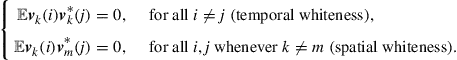 (9.6)
(9.6)
The noise process ![]() is further assumed to be independent of past signals
is further assumed to be independent of past signals ![]() across all nodes
across all nodes ![]() . Observe that we are allowing the noise power profile,
. Observe that we are allowing the noise power profile, ![]() , to vary with
, to vary with ![]() . In this way, the quality of the measurements is allowed to vary across the network with some nodes collecting noisier data than other nodes. Figure 9.3 illustrates an example of a network consisting of
. In this way, the quality of the measurements is allowed to vary across the network with some nodes collecting noisier data than other nodes. Figure 9.3 illustrates an example of a network consisting of ![]() nodes spread over a region in space. The figure shows the neighborhood of node
nodes spread over a region in space. The figure shows the neighborhood of node ![]() , which consists of nodes
, which consists of nodes ![]() .
.
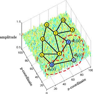
Figure 9.3 A collection of nodes, spread over a geographic region, observes realizations of an AR random process and cooperates to estimate the underlying model parameters ![]() in the presence of measurement noise. The noise power profile can vary over space.
in the presence of measurement noise. The noise power profile can vary over space.
3.09.2.1.1 Linear model
To illustrate the difference between cooperative and non-cooperative estimation strategies, let us first explain that the data can be represented in terms of a linear model. To do so, we collect the model parameters ![]() into an
into an ![]() column vector
column vector ![]() :
:
![]() (9.7)
(9.7)
and the past data into a ![]() row regression vector
row regression vector ![]() :
:
![]() (9.8)
(9.8)
Then, we can rewrite the measurement equation (9.4) at each node ![]() in the equivalent linear model form:
in the equivalent linear model form:
![]() (9.9)
(9.9)
Linear relations of the form (9.9) are common in applications and arise in many other contexts (as further illustrated by the next three examples in this section).
We assume the stochastic processes ![]() in (9.9) have zero means and are jointly wide-sense stationary. We denote their second-order moments by:
in (9.9) have zero means and are jointly wide-sense stationary. We denote their second-order moments by:
![]() (9.10)
(9.10)
![]() (9.11)
(9.11)
![]() (9.12)
(9.12)
As was the case with the noise power profile, we are allowing the moments ![]() to depend on the node index
to depend on the node index ![]() so that these moments can vary with the spatial dimension as well. The covariance matrix
so that these moments can vary with the spatial dimension as well. The covariance matrix ![]() is, by definition, always nonnegative definite. However, for convenience of presentation, we shall assume that
is, by definition, always nonnegative definite. However, for convenience of presentation, we shall assume that ![]() is actually positive-definite (and, hence, invertible):
is actually positive-definite (and, hence, invertible):
![]() (9.13)
(9.13)
3.09.2.1.2 Non-cooperative mean-square-error solution
One immediate result that follows from the linear model (9.9) is that the unknown parameter vector ![]() can be recovered exactly by each individual node from knowledge of the local moments
can be recovered exactly by each individual node from knowledge of the local moments ![]() alone. To see this, note that if we multiply both sides of (9.9) by
alone. To see this, note that if we multiply both sides of (9.9) by ![]() and take expectations we obtain
and take expectations we obtain
![]() (9.14)
(9.14)
so that
![]() (9.15)
(9.15)
It is seen from (9.15) that ![]() is the solution to a linear system of equations and that this solution can be computed by every node directly from its moments
is the solution to a linear system of equations and that this solution can be computed by every node directly from its moments ![]() . It is useful to re-interpret construction (9.15) as the solution to a minimum mean-square-error (MMSE) estimation problem [4,5]. Indeed, it can be verified that the quantity
. It is useful to re-interpret construction (9.15) as the solution to a minimum mean-square-error (MMSE) estimation problem [4,5]. Indeed, it can be verified that the quantity ![]() that appears in (9.15) is the unique solution to the following MMSE problem:
that appears in (9.15) is the unique solution to the following MMSE problem:
![]() (9.16)
(9.16)
To verify this claim, we denote the cost function that appears in (9.16) by
![]() (9.17)
(9.17)
and expand it to find that
![]() (9.18)
(9.18)
The cost function ![]() is quadratic in
is quadratic in ![]() and it has a unique minimizer since
and it has a unique minimizer since ![]() . Differentiating
. Differentiating ![]() with respect to
with respect to ![]() we find its gradient vector:
we find its gradient vector:
![]() (9.19)
(9.19)
It is seen that this gradient vector is annihilated at the same value ![]() given by (9.15). Therefore, we can equivalently state that if each node
given by (9.15). Therefore, we can equivalently state that if each node ![]() solves the MMSE problem (9.16), then the solution vector coincides with the desired parameter vector
solves the MMSE problem (9.16), then the solution vector coincides with the desired parameter vector ![]() . This observation explains why it is often justified to consider mean-square-error cost functions when dealing with estimation problems that involve data that satisfy linear models similar to (9.9).
. This observation explains why it is often justified to consider mean-square-error cost functions when dealing with estimation problems that involve data that satisfy linear models similar to (9.9).
Besides ![]() , the solution of the MMSE problem (9.16) also conveys information about the noise level in the data. Note that by substituting
, the solution of the MMSE problem (9.16) also conveys information about the noise level in the data. Note that by substituting ![]() from (9.15) into expression (9.16) for
from (9.15) into expression (9.16) for ![]() , the resulting minimum mean-square-error value that is attained by node
, the resulting minimum mean-square-error value that is attained by node ![]() is found to be:
is found to be:
 (9.20)
![]()
We shall use the notation ![]() and
and ![]() interchangeably to denote the minimum cost value of
interchangeably to denote the minimum cost value of ![]() . The above result states that, when each agent
. The above result states that, when each agent ![]() recovers
recovers ![]() from knowledge of its moments
from knowledge of its moments ![]() using expression (9.15), then the agent attains an MSE performance level that is equal to the noise power at its location,
using expression (9.15), then the agent attains an MSE performance level that is equal to the noise power at its location, ![]() . An alternative useful expression for the minimum cost can be obtained by substituting expression (9.15) for
. An alternative useful expression for the minimum cost can be obtained by substituting expression (9.15) for ![]() into (9.18) and simplifying the expression to find that
into (9.18) and simplifying the expression to find that
![]() (9.21)
(9.21)
This second expression is in terms of the data moments ![]() .
.
3.09.2.1.3 Non-cooperative adaptive solution
The optimal MMSE implementation (9.15) for determining ![]() requires knowledge of the statistical information
requires knowledge of the statistical information ![]() . This information is usually not available beforehand. Instead, the agents are more likely to have access to successive time-indexed observations
. This information is usually not available beforehand. Instead, the agents are more likely to have access to successive time-indexed observations ![]() of the random processes
of the random processes ![]() for
for ![]() . In this case, it becomes necessary to devise a scheme that would allow each node to use its measurements to approximate
. In this case, it becomes necessary to devise a scheme that would allow each node to use its measurements to approximate ![]() . It turns out that an adaptive solution is possible. In this alternative implementation, each node
. It turns out that an adaptive solution is possible. In this alternative implementation, each node ![]() feeds its observations
feeds its observations ![]() into an adaptive filter and evaluates successive estimates for
into an adaptive filter and evaluates successive estimates for ![]() . As time passes by, the estimates would get closer to
. As time passes by, the estimates would get closer to ![]() .
.
The adaptive solution operates as follows. Let ![]() denote an estimate for
denote an estimate for ![]() that is computed by node
that is computed by node ![]() at time
at time ![]() based on all the observations
based on all the observations ![]() it has collected up to that time instant. There are many adaptive algorithms that can be used to compute
it has collected up to that time instant. There are many adaptive algorithms that can be used to compute ![]() ; some filters are more accurate than others (usually, at the cost of additional complexity) [4–7]. It is sufficient for our purposes to consider one simple (yet effective) filter structure, while noting that most of the discussion in this chapter can be extended to other structures. One of the simplest choices for an adaptive structure is the least-mean-squares (LMS) filter, where the data are processed by each node
; some filters are more accurate than others (usually, at the cost of additional complexity) [4–7]. It is sufficient for our purposes to consider one simple (yet effective) filter structure, while noting that most of the discussion in this chapter can be extended to other structures. One of the simplest choices for an adaptive structure is the least-mean-squares (LMS) filter, where the data are processed by each node ![]() as follows:
as follows:
![]() (9.22)
(9.22)
![]() (9.23)
(9.23)
Starting from some initial condition, say, ![]() , the filter iterates over
, the filter iterates over ![]() . At each time instant,
. At each time instant, ![]() , the filter uses the local data
, the filter uses the local data ![]() at node
at node ![]() to compute a local estimation error,
to compute a local estimation error, ![]() , via (9.22). The error is then used to update the existing estimate from
, via (9.22). The error is then used to update the existing estimate from ![]() to
to ![]() via (9.23). The factor
via (9.23). The factor ![]() that appears in (9.23) is a constant positive step-size parameter; usually chosen to be sufficiently small to ensure mean-square stability and convergence, as discussed further ahead in the chapter. The step-size parameter can be selected to vary with time as well; one popular choice is to replace
that appears in (9.23) is a constant positive step-size parameter; usually chosen to be sufficiently small to ensure mean-square stability and convergence, as discussed further ahead in the chapter. The step-size parameter can be selected to vary with time as well; one popular choice is to replace ![]() in (9.23) with the following construction:
in (9.23) with the following construction:
![]() (9.24)
(9.24)
where ![]() is a small positive parameter and
is a small positive parameter and ![]() . The resulting filter implementation is known as normalized LMS [5] since the step-size is normalized by the squared norm of the regression vector. Other choices include step-size sequences
. The resulting filter implementation is known as normalized LMS [5] since the step-size is normalized by the squared norm of the regression vector. Other choices include step-size sequences ![]() that satisfy both conditions:
that satisfy both conditions:
![]() (9.25)
(9.25)
Such sequences converge slowly towards zero. One example is the choice ![]() . However, by virtue of the fact that such step-sizes die out as
. However, by virtue of the fact that such step-sizes die out as ![]() , then these choices end up turning off adaptation. As such, step-size sequences satisfying (9.25) are not generally suitable for applications that require continuous learning, especially under non-stationary environments. For this reason, in this chapter, we shall focus exclusively on the constant step-size case (9.23) in order to ensure continuous adaptation and learning.
, then these choices end up turning off adaptation. As such, step-size sequences satisfying (9.25) are not generally suitable for applications that require continuous learning, especially under non-stationary environments. For this reason, in this chapter, we shall focus exclusively on the constant step-size case (9.23) in order to ensure continuous adaptation and learning.
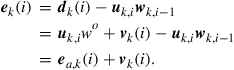
Equations (9.22) and (9.23) are written in terms of the observed quantities ![]() ; these are deterministic values since they correspond to observations of the random processes
; these are deterministic values since they correspond to observations of the random processes ![]() . Often, when we are interested in highlighting the random nature of the quantities involved in the adaptation step, especially when we study the mean-square performance of adaptive filters, it becomes more useful to rewrite the recursions using the boldface notation to highlight the fact that the quantities that appear in (9.22) and (9.23) are actually realizations of random variables. Thus, we also write:
. Often, when we are interested in highlighting the random nature of the quantities involved in the adaptation step, especially when we study the mean-square performance of adaptive filters, it becomes more useful to rewrite the recursions using the boldface notation to highlight the fact that the quantities that appear in (9.22) and (9.23) are actually realizations of random variables. Thus, we also write:
![]() (9.26)
(9.26)
![]() (9.27)
(9.27)
where ![]() will be random variables as well.
will be random variables as well.
The performance of adaptive implementations of this kind are well-understood for both cases of stationary ![]() and changing
and changing ![]() [4–7]. For example, in the stationary case, if the adaptive implementation (9.26) and (9.27) were to succeed in having its estimator
[4–7]. For example, in the stationary case, if the adaptive implementation (9.26) and (9.27) were to succeed in having its estimator ![]() tend to
tend to ![]() with probability one as
with probability one as ![]() , then we would expect the error signal
, then we would expect the error signal ![]() in (9.26) to tend towards the noise signal
in (9.26) to tend towards the noise signal ![]() (by virtue of the linear model (9.9)). This means that, under this ideal scenario, the variance of the error signal
(by virtue of the linear model (9.9)). This means that, under this ideal scenario, the variance of the error signal ![]() would be expected to tend towards the noise variance,
would be expected to tend towards the noise variance, ![]() , as
, as ![]() . Recall from (9.20) that the noise variance is the least cost that the MSE solution can attain. Therefore, such limiting behavior by the adaptive filter would be desirable. However, it is well-known that there is always some loss in mean-square-error performance when adaptation is employed due to the effect of gradient noise, which is caused by the algorithm’s reliance on observations (or realizations)
. Recall from (9.20) that the noise variance is the least cost that the MSE solution can attain. Therefore, such limiting behavior by the adaptive filter would be desirable. However, it is well-known that there is always some loss in mean-square-error performance when adaptation is employed due to the effect of gradient noise, which is caused by the algorithm’s reliance on observations (or realizations) ![]() rather than on the actual moments
rather than on the actual moments ![]() . In particular, it is known that for LMS filters, the variance of
. In particular, it is known that for LMS filters, the variance of ![]() in steady-state will be larger than
in steady-state will be larger than ![]() by a small amount, and the size of the offset is proportional to the step-size parameter
by a small amount, and the size of the offset is proportional to the step-size parameter ![]() (so that smaller step-sizes lead to better mean-square-error (MSE) performance albeit at the expense of slower convergence). It is easy to see why the variance of
(so that smaller step-sizes lead to better mean-square-error (MSE) performance albeit at the expense of slower convergence). It is easy to see why the variance of ![]() will be larger than
will be larger than ![]() from the definition of the error signal in (9.26). Introduce the weight-error vector
from the definition of the error signal in (9.26). Introduce the weight-error vector
![]() (9.28)
(9.28)
and the so-called a priori error signal
![]() (9.29)
(9.29)
This second error measures the difference between the uncorrupted term ![]() and its estimator prior to adaptation,
and its estimator prior to adaptation, ![]() . It then follows from the data model (9.9) and from the defining expression (9.26) for
. It then follows from the data model (9.9) and from the defining expression (9.26) for ![]() that
that
 (9.30)
Since the noise component, ![]() , is assumed to be zero-mean and independent of all other random variables, we conclude that
, is assumed to be zero-mean and independent of all other random variables, we conclude that
![]() (9.31)
(9.31)
This relation holds for any time instant ![]() ; it shows that the variance of the output error,
; it shows that the variance of the output error, ![]() is larger than
is larger than ![]() by an amount that is equal to the variance of the a priori error,
by an amount that is equal to the variance of the a priori error, ![]() . We define the filter mean-square-error (MSE) and excess-mean-square-error (EMSE) as the following steady-state measures:
. We define the filter mean-square-error (MSE) and excess-mean-square-error (EMSE) as the following steady-state measures:
![]() (9.32)
(9.32)
![]() (9.33)
(9.33)
so that, for the adaptive implementation (compare with (9.20)):
![]() (9.34)
(9.34)
Therefore, the EMSE term quantifies the size of the offset in the MSE performance of the adaptive filter. We also define the filter mean-square-deviation (MSD) as the steady-state measure:
![]() (9.35)
(9.35)
which measures how far ![]() is from
is from ![]() in the mean-square-error sense in steady-state. It is known that the MSD and EMSE of LMS filters of the form (9.26) and (9.27) can be approximated for sufficiently small-step sizes by the following expressions [4–7]:
in the mean-square-error sense in steady-state. It is known that the MSD and EMSE of LMS filters of the form (9.26) and (9.27) can be approximated for sufficiently small-step sizes by the following expressions [4–7]:
![]() (9.36)
(9.36)
![]() (9.37)
(9.37)
It is seen that the smaller the step-size parameter is, the better the performance of the adaptive solution.
3.09.2.1.4 Cooperative adaptation through diffusion
Observe from (9.36) and (9.37) that even if all nodes employ the same step-size, ![]() , and even if the regression data are spatially uniform so that
, and even if the regression data are spatially uniform so that ![]() for all
for all ![]() , the mean-square-error performance across the nodes still varies in accordance with the variation of the noise power profile,
, the mean-square-error performance across the nodes still varies in accordance with the variation of the noise power profile, ![]() , across the network. Nodes with larger noise power will perform worse than nodes with smaller noise power. However, since all nodes are observing data arising from the same underlying model
, across the network. Nodes with larger noise power will perform worse than nodes with smaller noise power. However, since all nodes are observing data arising from the same underlying model ![]() , it is natural to expect cooperation among the nodes to be beneficial. By cooperation we mean that neighboring nodes can share information (such as measurements or estimates) with each other as permitted by the network topology. Starting in the next section, we will motivate and describe algorithms that enable nodes to carry out adaptation and learning in a cooperative manner to enhance performance.
, it is natural to expect cooperation among the nodes to be beneficial. By cooperation we mean that neighboring nodes can share information (such as measurements or estimates) with each other as permitted by the network topology. Starting in the next section, we will motivate and describe algorithms that enable nodes to carry out adaptation and learning in a cooperative manner to enhance performance.
Specifically, we are going to see that one way to achieve cooperation is by developing adaptive algorithms that enable the nodes to optimize the following global cost function in a distributed manner:
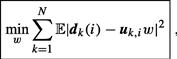 (9.38)
where the global cost is the aggregate objective:
 (9.39)
Comparing (9.38) with (9.16), we see that we are now adding the individual costs, ![]() , from across all nodes. Note that since the desired
, from across all nodes. Note that since the desired ![]() satisfies (9.15) at every node
satisfies (9.15) at every node ![]() , then it also satisfies
, then it also satisfies
 (9.40)
But it can be verified that the optimal solution to (9.38) is given by the same ![]() that satisfies (9.40). Therefore, solving the global optimization problem (9.38) also leads to the desired
that satisfies (9.40). Therefore, solving the global optimization problem (9.38) also leads to the desired ![]() . In future sections, we will show how cooperative and distributed adaptive schemes for solving (9.38), such as (9.153) or (9.154) further ahead, lead to improved performance in estimating
. In future sections, we will show how cooperative and distributed adaptive schemes for solving (9.38), such as (9.153) or (9.154) further ahead, lead to improved performance in estimating ![]() (in terms of smaller mean-square-deviation and faster convergence rate) than the non-cooperative mode (9.26) and (9.27), where each agent runs its own individual adaptive filter—see, e.g., Theorems 9.6.3–9.6.5 and Section 3.09.7.3.
(in terms of smaller mean-square-deviation and faster convergence rate) than the non-cooperative mode (9.26) and (9.27), where each agent runs its own individual adaptive filter—see, e.g., Theorems 9.6.3–9.6.5 and Section 3.09.7.3.
3.09.2.2 Application: tapped-delay-line models
Our second example to motivate MSE cost functions, ![]() , and linear models relates to identifying the parameters of a moving-average (MA) model from noisy data. MA models are also known as finite-impulse-response (FIR) or tapped-delay-line models. Thus, consider a situation where agents are interested in estimating the parameters of an FIR model, such as the taps of a communications channel or the parameters of some (approximate) model of interest in finance or biology. Assume the agents are able to independently probe the unknown model and observe its response to excitations in the presence of additive noise; this situation is illustrated in Figure 9.4, with the probing operation highlighted for one of the nodes (node 4).
, and linear models relates to identifying the parameters of a moving-average (MA) model from noisy data. MA models are also known as finite-impulse-response (FIR) or tapped-delay-line models. Thus, consider a situation where agents are interested in estimating the parameters of an FIR model, such as the taps of a communications channel or the parameters of some (approximate) model of interest in finance or biology. Assume the agents are able to independently probe the unknown model and observe its response to excitations in the presence of additive noise; this situation is illustrated in Figure 9.4, with the probing operation highlighted for one of the nodes (node 4).
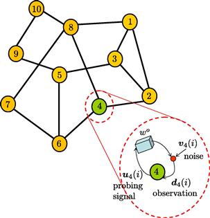
Figure 9.4 The network is interested in estimating the parameter vector ![]() that describes an underlying tapped-delay-line model. The agents are assumed to be able to independently probe the unknown system, and observe its response to excitations, under noise, as indicated in the highlighted diagram for node
that describes an underlying tapped-delay-line model. The agents are assumed to be able to independently probe the unknown system, and observe its response to excitations, under noise, as indicated in the highlighted diagram for node ![]() .
.
The schematics inside the enlarged diagram in Figure 9.4 is meant to convey that each node ![]() probes the model with an input sequence
probes the model with an input sequence ![]() and measures the resulting response sequence,
and measures the resulting response sequence, ![]() , in the presence of additive noise. The system dynamics for each agent
, in the presence of additive noise. The system dynamics for each agent ![]() is assumed to be described by a MA model of the form:
is assumed to be described by a MA model of the form:
 (9.41)
In this model, the term ![]() again represents an additive zero-mean noise process that is assumed to be temporally white and spatially independent; it is also assumed to be independent of the input process,
again represents an additive zero-mean noise process that is assumed to be temporally white and spatially independent; it is also assumed to be independent of the input process, ![]() , for all
, for all ![]() , and
, and ![]() . The scalars
. The scalars ![]() represent the model parameters that the agents seek to identify. If we again collect the model parameters into an
represent the model parameters that the agents seek to identify. If we again collect the model parameters into an ![]() column vector
column vector ![]() :
:
![]() (9.42)
(9.42)
and the input data into a ![]() row regression vector:
row regression vector:
![]() (9.43)
(9.43)
then, we can again express the measurement equation (9.41) at each node ![]() in the same linear model as (9.9), namely,
in the same linear model as (9.9), namely,
![]() (9.44)
(9.44)
As was the case with model (9.9), we can likewise verify that, in view of (9.44), the desired parameter vector ![]() satisfies the same normal equations (9.15), i.e.,
satisfies the same normal equations (9.15), i.e.,
![]() (9.45)
(9.45)
where the moments ![]() continue to be defined by expressions (9.11) and (9.12) with
continue to be defined by expressions (9.11) and (9.12) with ![]() now defined by (9.43). Therefore, each node
now defined by (9.43). Therefore, each node ![]() can determine
can determine ![]() on its own by solving the same MMSE estimation problem (9.16). This solution method requires knowledge of the moments
on its own by solving the same MMSE estimation problem (9.16). This solution method requires knowledge of the moments ![]() and, according to (9.20), each agent
and, according to (9.20), each agent ![]() would then attain an MSE level that is equal to the noise power level at its location.
would then attain an MSE level that is equal to the noise power level at its location.
Alternatively, when the statistical information ![]() is not available, each agent
is not available, each agent ![]() can estimate
can estimate ![]() iteratively by feeding data
iteratively by feeding data ![]() into the adaptive implementation (9.26) and (9.27). In this way, each agent
into the adaptive implementation (9.26) and (9.27). In this way, each agent ![]() will achieve the same performance level shown earlier in (9.36) and (9.37), with the limiting performance being again dependent on the local noise power level,
will achieve the same performance level shown earlier in (9.36) and (9.37), with the limiting performance being again dependent on the local noise power level, ![]() . Therefore, nodes with larger noise power will perform worse than nodes with smaller noise power. However, since all nodes are observing data arising from the same underlying model
. Therefore, nodes with larger noise power will perform worse than nodes with smaller noise power. However, since all nodes are observing data arising from the same underlying model ![]() , it is natural to expect cooperation among the nodes to be beneficial. As we are going to see, starting from the next section, one way to achieve cooperation and improve performance is by developing algorithms that optimize the same global cost function (9.38) in an adaptive and distributed manner, such as algorithms (9.153) and (9.154) further ahead.
, it is natural to expect cooperation among the nodes to be beneficial. As we are going to see, starting from the next section, one way to achieve cooperation and improve performance is by developing algorithms that optimize the same global cost function (9.38) in an adaptive and distributed manner, such as algorithms (9.153) and (9.154) further ahead.
3.09.2.3 Application: target localization
Our third example relates to the problem of locating a destination of interest (such as the location of a nutrition source or a chemical leak) or locating and tracking an object of interest (such as a predator or a projectile). In several such localization applications, the agents in the network are allowed to move towards the target or away from it, in which case we would end up with a mobile adaptive network [8]. Biological networks behave in this manner such as networks representing fish schools, bird formations, bee swarms, bacteria motility, and diffusing particles [8–12]. The agents may move towards the target (e.g., when it is a nutrition source) or away from the target (e.g., when it is a predator). In other applications, the agents may remain static and are simply interested in locating a target or tracking it (such as tracking a projectile).
To motivate mean-square-error estimation in the context of localization problems, we consider the situation corresponding to a static target and static nodes. Thus, assume that the unknown location of the target in the cartesian plane is represented by the ![]() vector
vector ![]() . The agents are spread over the same region of space and are interested in locating the target. The location of every agent
. The agents are spread over the same region of space and are interested in locating the target. The location of every agent ![]() is denoted by the
is denoted by the ![]() vector
vector ![]() in terms of its
in terms of its ![]() and
and ![]() coordinates—see Figure 9.5. We assume the agents are aware of their location vectors. The distance between agent
coordinates—see Figure 9.5. We assume the agents are aware of their location vectors. The distance between agent ![]() and the target is denoted by
and the target is denoted by ![]() and is equal to:
and is equal to:
![]() (9.46)
(9.46)
The ![]() unit-norm direction vector pointing from agent
unit-norm direction vector pointing from agent ![]() towards the target is denoted by
towards the target is denoted by ![]() and is given by:
and is given by:
![]() (9.47)
(9.47)
Observe from (9.46) and (9.47) that ![]() can be expressed in the following useful inner-product form:
can be expressed in the following useful inner-product form:
![]() (9.48)
(9.48)

Figure 9.5 The distance from node ![]() to the target is denoted by
to the target is denoted by ![]() and the unit-norm direction vector from the same node to the target is denoted by
and the unit-norm direction vector from the same node to the target is denoted by ![]() . Node
. Node ![]() is assumed to have access to noisy measurements of
is assumed to have access to noisy measurements of ![]() .
.
In practice, agents have noisy observations of both their distance and direction vector towards the target. We denote the noisy distance measurement collected by node ![]() at time
at time ![]() by:
by:
![]() (9.49)
(9.49)
where ![]() denotes noise and is assumed to be zero-mean, and temporally white and spatially in-dependent with variance
denotes noise and is assumed to be zero-mean, and temporally white and spatially in-dependent with variance
![]() (9.50)
(9.50)
We also denote the noisy direction vector that is measured by node ![]() at time
at time ![]() by
by ![]() . This vector is a perturbed version of
. This vector is a perturbed version of ![]() . We assume that
. We assume that ![]() continues to start from the location of the node at
continues to start from the location of the node at ![]() , but that its tip is perturbed slightly either to the left or to the right relative to the tip of
, but that its tip is perturbed slightly either to the left or to the right relative to the tip of ![]() —see Figure 9.6. The perturbation to the tip of
—see Figure 9.6. The perturbation to the tip of ![]() is modeled as being the result of two effects: a small deviation that occurs along the direction that is perpendicular to
is modeled as being the result of two effects: a small deviation that occurs along the direction that is perpendicular to ![]() , and a smaller deviation that occurs along the direction of
, and a smaller deviation that occurs along the direction of ![]() . Since we are assuming that the tip of
. Since we are assuming that the tip of ![]() is only slightly perturbed relative to the tip of
is only slightly perturbed relative to the tip of ![]() , then it is reasonable to expect the amount of perturbation along the parallel direction to be small compared to the amount of perturbation along the perpendicular direction.
, then it is reasonable to expect the amount of perturbation along the parallel direction to be small compared to the amount of perturbation along the perpendicular direction.
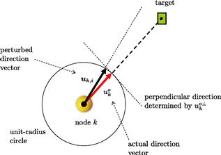
Figure 9.6 The tip of the noisy direction vector is modeled as being approximately perturbed away from the actual direction by two effects: a larger effect caused by a deviation along the direction that is perpendicular to ![]() , and a smaller deviation along the direction that is parallel to
, and a smaller deviation along the direction that is parallel to ![]() .
.
Thus, we write
![]() (9.51)
(9.51)
where ![]() denotes a unit-norm row vector that lies in the same plane and whose direction is perpendicular to
denotes a unit-norm row vector that lies in the same plane and whose direction is perpendicular to ![]() . The variables
. The variables ![]() and
and ![]() denote zero-mean independent random noises that are temporally white and spatially independent with variances:
denote zero-mean independent random noises that are temporally white and spatially independent with variances:
![]() (9.52)
(9.52)
We assume the contribution of ![]() is small compared to the contributions of the other noise sources,
is small compared to the contributions of the other noise sources, ![]() and
and ![]() , so that
, so that
![]() (9.53)
(9.53)
The random noises ![]() are further assumed to be independent of each other.
are further assumed to be independent of each other.
Using (9.48) we find that the noisy measurements ![]() are related to the unknown
are related to the unknown ![]() via:
via:
![]() (9.54)
(9.54)
where the modified noise term ![]() is defined in terms of the noises in
is defined in terms of the noises in ![]() and
and ![]() as follows:
as follows:
 (9.55)
since, by construction,
![]() (9.56)
(9.56)
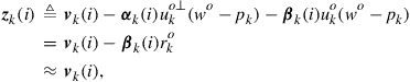
and the contribution by ![]() is assumed to be sufficiently small. If we now introduce the adjusted signal:
is assumed to be sufficiently small. If we now introduce the adjusted signal:
![]() (9.57)
(9.57)
then we arrive again from (9.54) and (9.55) at the following linear model for the available measurement variables ![]() in terms of the target location
in terms of the target location ![]() :
:
![]() (9.58)
(9.58)
There is one important difference in relation to the earlier linear models (9.9) and (9.44), namely, the variables ![]() in (9.58) do not have zero means any longer. It is nevertheless straightforward to determine the first and second-order moments of the variables
in (9.58) do not have zero means any longer. It is nevertheless straightforward to determine the first and second-order moments of the variables ![]() . First, note from (9.49), (9.51), and (9.57) that
. First, note from (9.49), (9.51), and (9.57) that
![]() (9.59)
(9.59)
Even in this case of non-zero means, and in view of (9.58), the desired parameter vector ![]() can still be shown to satisfy the same normal equations (9.15), i.e.,
can still be shown to satisfy the same normal equations (9.15), i.e.,
![]() (9.60)
(9.60)
where the moments ![]() continue to be defined as
continue to be defined as
![]() (9.61)
(9.61)
To verify that (9.60) holds, we simply multiply both sides of (9.58) by ![]() from the left, compute the expectations of both sides, and use the fact that
from the left, compute the expectations of both sides, and use the fact that ![]() has zero mean and is assumed to be independent of
has zero mean and is assumed to be independent of ![]() for all times
for all times ![]() and nodes
and nodes ![]() . However, the difference in relation to the earlier normal equations (9.15) is that the matrix
. However, the difference in relation to the earlier normal equations (9.15) is that the matrix ![]() is not the actual covariance matrix of
is not the actual covariance matrix of ![]() any longer. When
any longer. When ![]() is not zero mean, its covariance matrix is instead defined as:
is not zero mean, its covariance matrix is instead defined as:
![]() (9.62)
(9.62)
so that
![]() (9.63)
(9.63)
We conclude from this relation that ![]() is positive-definite (and, hence, invertible) so that expression (9.60) is justified. This is because the covariance matrix,
is positive-definite (and, hence, invertible) so that expression (9.60) is justified. This is because the covariance matrix, ![]() , is itself positive-definite. Indeed, some algebra applied to the difference
, is itself positive-definite. Indeed, some algebra applied to the difference ![]() from (9.51) shows that
from (9.51) shows that
 (9.64)
where the matrix
 (9.65)
is full rank since the rows ![]() are linearly independent vectors.
are linearly independent vectors.
Therefore, each node ![]() can determine
can determine ![]() on its own by solving the same minimum mean-square-error estimation problem (9.16). This solution method requires knowledge of the moments
on its own by solving the same minimum mean-square-error estimation problem (9.16). This solution method requires knowledge of the moments ![]() and, according to (9.20), each agent
and, according to (9.20), each agent ![]() would then attain an MSE level that is equal to the noise power level,
would then attain an MSE level that is equal to the noise power level, ![]() , at its location.
, at its location.
Alternatively, when the statistical information ![]() is not available beforehand, each agent
is not available beforehand, each agent ![]() can estimate
can estimate ![]() iteratively by feeding data
iteratively by feeding data ![]() into the adaptive implementation (9.26) and (9.27). In this case, each agent
into the adaptive implementation (9.26) and (9.27). In this case, each agent ![]() will achieve the performance level shown earlier in (9.36) and (9.37), with the limiting performance being again dependent on the local noise power level,
will achieve the performance level shown earlier in (9.36) and (9.37), with the limiting performance being again dependent on the local noise power level, ![]() . Therefore, nodes with larger noise power will perform worse than nodes with smaller noise power. However, since all nodes are observing distances and direction vectors towards the same target location
. Therefore, nodes with larger noise power will perform worse than nodes with smaller noise power. However, since all nodes are observing distances and direction vectors towards the same target location ![]() , it is natural to expect cooperation among the nodes to be beneficial. As we are going to see, starting from the next section, one way to achieve cooperation and improve performance is by developing algorithms that solve the same global cost function (9.38) in an adaptive and distributed manner, by using algorithms such as (9.153) and (9.154) further ahead.
, it is natural to expect cooperation among the nodes to be beneficial. As we are going to see, starting from the next section, one way to achieve cooperation and improve performance is by developing algorithms that solve the same global cost function (9.38) in an adaptive and distributed manner, by using algorithms such as (9.153) and (9.154) further ahead.
3.09.2.3.1 Role of adaptation
The localization application helps highlight one of the main advantages of adaptation, namely, the ability of adaptive implementations to learn and track changing statistical conditions. For example, in the context of mobile networks, where nodes can move closer or further away from a target, the location vector for each agent ![]() becomes time-dependent, say,
becomes time-dependent, say, ![]() . In this case, the actual distance and direction vector between agent
. In this case, the actual distance and direction vector between agent ![]() and the target also vary with time and become:
and the target also vary with time and become:
![]() (9.66)
(9.66)
The noisy distance measurement to the target is then:
![]() (9.67)
(9.67)
where the variance of ![]() now depends on time as well:
now depends on time as well:
![]() (9.68)
(9.68)
In the context of mobile networks, it is reasonable to assume that the variance of ![]() varies both with time and with the distance to the target: the closer the node is to the target, the less noisy the measurement of the distance is expected to be. Similar remarks hold for the variances of the noises
varies both with time and with the distance to the target: the closer the node is to the target, the less noisy the measurement of the distance is expected to be. Similar remarks hold for the variances of the noises ![]() and
and ![]() that perturb the measurement of the direction vector, say,
that perturb the measurement of the direction vector, say,
![]() (9.69)
(9.69)
where now
![]() (9.70)
(9.70)
The same arguments that led to (9.58) can be repeated to lead to the same model, except that now the means of the variables ![]() become time-dependent as well:
become time-dependent as well:
![]() (9.71)
(9.71)
Nevertheless, adaptive solutions (whether cooperative or non-cooperative), are able to track such time-variations because these solutions work directly with the observations ![]() and the successive observations will reflect the changing statistical profile of the data. In general, adaptive solutions are able to track changes in the underlying signal statistics rather well [4,5], as long as the rate of non-stationarity is slow enough for the filter to be able to follow the changes.
and the successive observations will reflect the changing statistical profile of the data. In general, adaptive solutions are able to track changes in the underlying signal statistics rather well [4,5], as long as the rate of non-stationarity is slow enough for the filter to be able to follow the changes.
3.09.2.4 Application: collaborative spectral sensing
Our fourth and last example to illustrate the role of mean-square-error estimation and cooperation relates to spectrum sensing for cognitive radio applications. Cognitive radio systems involve two types of users: primary users and secondary users. To avoid causing harmful interference to incumbent primary users, unlicensed cognitive radio devices need to detect unused frequency bands even at low signal-to-noise (SNR) conditions [13–16]. One way to carry out spectral sensing is for each secondary user to estimate the aggregated power spectrum that is transmitted by all active primary users, and to locate unused frequency bands within the estimated spectrum. This step can be performed by the secondary users with or without cooperation.
Thus, consider a communications environment consisting of ![]() primary users and
primary users and ![]() secondary users. Let
secondary users. Let ![]() denote the power spectrum of the signal transmitted by primary user
denote the power spectrum of the signal transmitted by primary user ![]() . To facilitate estimation of the spectral profile by the secondary users, we assume that each
. To facilitate estimation of the spectral profile by the secondary users, we assume that each ![]() can be represented as a linear combination of some basis functions,
can be represented as a linear combination of some basis functions, ![]() , say,
, say, ![]() of them [17]:
of them [17]:
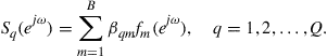 (9.72)
In this representation, the scalars ![]() denote the coefficients of the basis expansion for user
denote the coefficients of the basis expansion for user ![]() . The variable
. The variable ![]() denotes the normalized angular frequency measured in radians/sample. The power spectrum is often symmetric about the vertical axis,
denotes the normalized angular frequency measured in radians/sample. The power spectrum is often symmetric about the vertical axis, ![]() , and therefore it is sufficient to focus on the interval
, and therefore it is sufficient to focus on the interval ![]() . There are many ways by which the basis functions,
. There are many ways by which the basis functions, ![]() , can be selected. The following is one possible construction for illustration purposes. We divide the interval
, can be selected. The following is one possible construction for illustration purposes. We divide the interval ![]() into
into ![]() identical intervals and denote their center frequencies by
identical intervals and denote their center frequencies by ![]() . We then place a Gaussian pulse at each location
. We then place a Gaussian pulse at each location ![]() and control its width through the selection of its standard deviation,
and control its width through the selection of its standard deviation, ![]() , i.e.,
, i.e.,
![]() (9.73)
(9.73)
Figure 9.7 illustrates this construction. The parameters ![]() are selected by the designer and are assumed to be known. For a sufficiently large number,
are selected by the designer and are assumed to be known. For a sufficiently large number, ![]() , of basis functions, the representation (9.72) can approximate well a large class of power spectra.
, of basis functions, the representation (9.72) can approximate well a large class of power spectra.

Figure 9.7 The interval ![]() is divided into
is divided into ![]() sub-intervals of equal width; the center frequencies of the sub-intervals are denoted by
sub-intervals of equal width; the center frequencies of the sub-intervals are denoted by ![]() . A power spectrum
. A power spectrum ![]() is approximated as a linear combination of Gaussian basis functions centered on the
is approximated as a linear combination of Gaussian basis functions centered on the ![]() .
.
We collect the combination coefficients ![]() for primary user
for primary user ![]() into a column vector
into a column vector ![]() :
:
![]() (9.74)
(9.74)
and collect the basis functions into a row vector:
![]() (9.75)
(9.75)
Then, the power spectrum (9.72) can be expressed in the alternative inner-product form:
![]() (9.76)
(9.76)
Let ![]() denote the path loss coefficient from primary user
denote the path loss coefficient from primary user ![]() to secondary user
to secondary user ![]() . When the transmitted spectrum
. When the transmitted spectrum ![]() travels from primary user
travels from primary user ![]() to secondary user
to secondary user ![]() , the spectrum that is sensed by node
, the spectrum that is sensed by node ![]() is
is ![]() . We assume in this example that the path loss factors
. We assume in this example that the path loss factors ![]() are known and that they have been determined during a prior training stage involving each of the primary users with each of the secondary users. The training is usually repeated at regular intervals of time to accommodate the fact that the path loss coefficients can vary (albeit slowly) over time. Figure 9.8 depicts a cognitive radio system with
are known and that they have been determined during a prior training stage involving each of the primary users with each of the secondary users. The training is usually repeated at regular intervals of time to accommodate the fact that the path loss coefficients can vary (albeit slowly) over time. Figure 9.8 depicts a cognitive radio system with ![]() primary users and
primary users and ![]() secondary users. One of the secondary users (user
secondary users. One of the secondary users (user ![]() ) is highlighted and the path loss coefficients from the primary users to its location are indicated; similar path loss coefficients can be assigned to all other combinations involving primary and secondary users.
) is highlighted and the path loss coefficients from the primary users to its location are indicated; similar path loss coefficients can be assigned to all other combinations involving primary and secondary users.
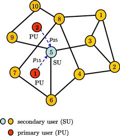
Figure 9.8 A network of secondary users in the presence of two primary users. One of the secondary users is highlighted and the path loss coefficients from the primary users to its location are indicated as ![]() and
and ![]() .
.
Each user ![]() senses the aggregate effect of the power spectra that are transmitted by all active primary users. Therefore, adding the effect of all primary users, we find that the power spectrum that arrives at secondary user
senses the aggregate effect of the power spectra that are transmitted by all active primary users. Therefore, adding the effect of all primary users, we find that the power spectrum that arrives at secondary user ![]() is given by:
is given by:
 (9.77)
where ![]() denotes the receiver noise power at node
denotes the receiver noise power at node ![]() , and where we introduced the following vector quantities:
, and where we introduced the following vector quantities:
![]() (9.78)
(9.78)
![]() (9.79)
(9.79)
The vector ![]() is the collection of all combination coefficients for all
is the collection of all combination coefficients for all ![]() primary users. The vector
primary users. The vector ![]() contains the path loss coefficients from all primary users to user
contains the path loss coefficients from all primary users to user ![]() . Now, at every time instant
. Now, at every time instant ![]() , user
, user ![]() observers its received power spectrum,
observers its received power spectrum, ![]() , over a discrete grid of frequencies,
, over a discrete grid of frequencies, ![]() , in the interval
, in the interval ![]() in the presence of additive measurement noise. We denote these measurements by:
in the presence of additive measurement noise. We denote these measurements by:
![]() (9.80)
(9.80)
The term ![]() denotes sampling noise and is assumed to have zero mean and variance
denotes sampling noise and is assumed to have zero mean and variance ![]() ; it is also assumed to be temporally white and spatially independent; and is also independent of all other random variables. Since the row vectors
; it is also assumed to be temporally white and spatially independent; and is also independent of all other random variables. Since the row vectors ![]() in (9.79) are defined in terms of the path loss coefficients
in (9.79) are defined in terms of the path loss coefficients ![]() , and since these coefficients are estimated and subject to noisy distortions, we model the
, and since these coefficients are estimated and subject to noisy distortions, we model the ![]() as zero-mean random variables in (9.80) and use the boldface notation for them.
as zero-mean random variables in (9.80) and use the boldface notation for them.
Observe that in this application, each node ![]() collects
collects ![]() measurements at every time instant
measurements at every time instant ![]() and not only a single measurement, as was the case with the three examples discussed in the previous sections (AR modeling, MA modeling, and localization). The implication of this fact is that we now deal with an estimation problem that involves vector measurements instead of scalar measurements at each node. The solution structure continues to be the same. We collect the
and not only a single measurement, as was the case with the three examples discussed in the previous sections (AR modeling, MA modeling, and localization). The implication of this fact is that we now deal with an estimation problem that involves vector measurements instead of scalar measurements at each node. The solution structure continues to be the same. We collect the ![]() measurements at node
measurements at node ![]() at time
at time ![]() into vectors and introduce the
into vectors and introduce the ![]() quantities:
quantities:
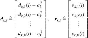 (9.81)
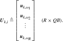 (9.82)
The time subscript in ![]() is used to model the fact that the path loss coefficients can change over time due to the possibility of node mobility. With the above notation, expression (9.80) is equivalent to the linear model:
is used to model the fact that the path loss coefficients can change over time due to the possibility of node mobility. With the above notation, expression (9.80) is equivalent to the linear model:
![]() (9.83)
(9.83)
Compared to the earlier examples (9.9), (9.44), and (9.58), the main difference now is that each agent ![]() collects a vector of measurements,
collects a vector of measurements, ![]() , as opposed to the scalar
, as opposed to the scalar ![]() , and its regression data are represented by the matrix quantity,
, and its regression data are represented by the matrix quantity, ![]() , as opposed to the row vector
, as opposed to the row vector ![]() . Nevertheless, the estimation approach will continue to be the same. In cognitive network applications, the secondary users are interested in estimating the aggregate power spectrum of the primary users in order for the secondary users to identify vacant frequency bands that can be used by them. In the context of model (9.83), this amounts to determining the parameter vector
. Nevertheless, the estimation approach will continue to be the same. In cognitive network applications, the secondary users are interested in estimating the aggregate power spectrum of the primary users in order for the secondary users to identify vacant frequency bands that can be used by them. In the context of model (9.83), this amounts to determining the parameter vector ![]() since knowledge of its entries allows each secondary user to reconstruct the aggregate power spectrum defined by:
since knowledge of its entries allows each secondary user to reconstruct the aggregate power spectrum defined by:
 (9.84)
where the notation ![]() denotes the Kronecker product operation, and
denotes the Kronecker product operation, and ![]() denotes a
denotes a ![]() vector whose entries are all equal to one.
vector whose entries are all equal to one.
As before, we can again verify that, in view of (9.83), the desired parameter vector ![]() satisfies the same normal equations:
satisfies the same normal equations:
![]() (9.85)
(9.85)
where the moments ![]() are now defined by
are now defined by
![]() (9.86)
(9.86)
![]() (9.87)
(9.87)
Therefore, each secondary user ![]() can determine
can determine ![]() on its own by solving the following minimum mean-square-error estimation problem:
on its own by solving the following minimum mean-square-error estimation problem:
![]() (9.88)
(9.88)
This solution method requires knowledge of the moments ![]() and, in an argument similar to the one that led to (9.20), it can be verified that each agent
and, in an argument similar to the one that led to (9.20), it can be verified that each agent ![]() would attain an MSE performance level that is equal to the noise power level,
would attain an MSE performance level that is equal to the noise power level, ![]() , at its location.
, at its location.
Alternatively, when the statistical information ![]() is not available, each secondary user
is not available, each secondary user ![]() can estimate
can estimate ![]() iteratively by feeding data
iteratively by feeding data ![]() into an adaptive implementation similar to (9.26) and (9.27), such as the following vector LMS recursion:
into an adaptive implementation similar to (9.26) and (9.27), such as the following vector LMS recursion:
![]() (9.89)
(9.89)
![]() (9.90)
(9.90)
In this case, each secondary user ![]() will achieve performance levels similar to (9.36) and (9.37) with
will achieve performance levels similar to (9.36) and (9.37) with ![]() replaced by
replaced by ![]() and
and ![]() replaced by
replaced by ![]() . The performance will again be dependent on the local noise level,
. The performance will again be dependent on the local noise level, ![]() . As a result, secondary users with larger noise power will perform worse than secondary users with smaller noise power. However, since all secondary users are observing data arising from the same underlying model
. As a result, secondary users with larger noise power will perform worse than secondary users with smaller noise power. However, since all secondary users are observing data arising from the same underlying model ![]() , it is natural to expect cooperation among the users to be beneficial. As we are going to see, starting from the next section, one way to achieve cooperation and improve performance is by developing algorithms that solve the following global cost function in an adaptive and distributed manner:
, it is natural to expect cooperation among the users to be beneficial. As we are going to see, starting from the next section, one way to achieve cooperation and improve performance is by developing algorithms that solve the following global cost function in an adaptive and distributed manner:
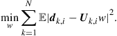 (9.91)
3.09.3 Distributed optimization via diffusion strategies
The examples in the previous section were meant to illustrate how MSE cost functions and linear models are useful design tools and how they arise frequently in applications. We now return to problem (9.1) and study the distributed optimization of global cost functions such as (9.39), where ![]() is assumed to consist of the sum of individual components. Specifically, we are now interested in solving optimization problems of the type:
is assumed to consist of the sum of individual components. Specifically, we are now interested in solving optimization problems of the type:
 (9.92)
where each ![]() is assumed to be differentiable and convex over
is assumed to be differentiable and convex over ![]() . Although the algorithms presented in this chapter apply to more general situations, we shall nevertheless focus on mean-square-error cost functions of the form:
. Although the algorithms presented in this chapter apply to more general situations, we shall nevertheless focus on mean-square-error cost functions of the form:
![]() (9.93)
(9.93)
where ![]() is an
is an ![]() column vector, and the random processes
column vector, and the random processes ![]() are assumed to be jointly wide-sense stationary with zero-mean and second-order moments:
are assumed to be jointly wide-sense stationary with zero-mean and second-order moments:
![]() (9.94)
(9.94)
![]() (9.95)
(9.95)
![]() (9.96)
(9.96)
It is clear that each ![]() is quadratic in
is quadratic in ![]() since, after expansion, we get
since, after expansion, we get
![]() (9.97)
(9.97)
A completion-of-squares argument shows that ![]() can be expressed as the sum of two squared terms, i.e.,
can be expressed as the sum of two squared terms, i.e.,
![]() (9.98)
(9.98)
or, more compactly,
![]() (9.99)
(9.99)
where ![]() denotes the minimizer of
denotes the minimizer of ![]() and is given by
and is given by
![]() (9.100)
(9.100)
and ![]() denotes the minimum value of
denotes the minimum value of ![]() when evaluated at
when evaluated at ![]() :
:
![]() (9.101)
(9.101)
Observe that this value is necessarily nonnegative since it can be viewed as the Schur complement of the following covariance matrix:
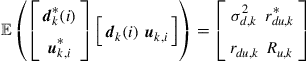 (9.102)
and covariance matrices are nonnegative-definite.
The choice of the quadratic form (9.93) or (9.97) for ![]() is useful for many applications, as was already illustrated in the previous section for examples involving AR modeling, MA modeling, localization, and spectral sensing. Other choices for
is useful for many applications, as was already illustrated in the previous section for examples involving AR modeling, MA modeling, localization, and spectral sensing. Other choices for ![]() are of course possible and these choices can even be different for different nodes. It is sufficient in this chapter to illustrate the main concepts underlying diffusion adaptation by focusing on the useful case of MSE cost functions of the form (9.97); still, most of the derivations and arguments in the coming sections can be extended beyond MSE optimization to more general cost functions and to situations where the minimizers of the individual costs do not necessarily occur at the same location—as already shown in [1–3]; see also Section 3.09.10.4.
are of course possible and these choices can even be different for different nodes. It is sufficient in this chapter to illustrate the main concepts underlying diffusion adaptation by focusing on the useful case of MSE cost functions of the form (9.97); still, most of the derivations and arguments in the coming sections can be extended beyond MSE optimization to more general cost functions and to situations where the minimizers of the individual costs do not necessarily occur at the same location—as already shown in [1–3]; see also Section 3.09.10.4.
The positive-definiteness of the covariance matrices ![]() ensures that each
ensures that each ![]() in (9.97) is strictly convex, as well as
in (9.97) is strictly convex, as well as ![]() from (9.39). Moreover, all these cost functions have a unique minimum at the same
from (9.39). Moreover, all these cost functions have a unique minimum at the same ![]() , which satisfies the normal equations:
, which satisfies the normal equations:
![]() (9.103)
(9.103)
Therefore, given knowledge of ![]() , each node can determine
, each node can determine ![]() on its own by solving (9.103). One then wonders about the need to seek distributed cooperative and adaptive solutions in this case. There are a couple of reasons:
on its own by solving (9.103). One then wonders about the need to seek distributed cooperative and adaptive solutions in this case. There are a couple of reasons:
a. First, even for MSE cost functions, it is often the case that the required moments ![]() are not known beforehand. In this case, the optimal
are not known beforehand. In this case, the optimal ![]() cannot be determined from the solution of the normal equations (9.103). The alternative methods that we shall describe will lead to adaptive techniques that enable each node
cannot be determined from the solution of the normal equations (9.103). The alternative methods that we shall describe will lead to adaptive techniques that enable each node ![]() to estimate
to estimate ![]() directly from data realizations.
directly from data realizations.
b. Second, since adaptive strategies rely on instantaneous data, these strategies possess powerful tracking abilities. Even when the moments vary with time due to non-stationary behavior (such as ![]() changing with time), these changes will be reflected in the observed data and will in turn influence the behavior of the adaptive construction. This is one of the key advantages of adaptive strategies: they enable learning and tracking in real-time.
changing with time), these changes will be reflected in the observed data and will in turn influence the behavior of the adaptive construction. This is one of the key advantages of adaptive strategies: they enable learning and tracking in real-time.
c. Third, cooperation among nodes is generally beneficial. When nodes act individually, their performance is limited by the noise power level at their location. In this way, some nodes can perform significantly better than other nodes. On the other hand, when nodes cooperate with their neighbors and share information during the adaptation process, we will see that performance can be improved across the network.
3.09.3.1 Relating the global cost to neighborhood costs
Let us therefore consider the optimization of the following global cost function:
 (9.104)
where ![]() is given by (9.93) or (9.97)(9.93) or (9.97). Our strategy to optimize
is given by (9.93) or (9.97)(9.93) or (9.97). Our strategy to optimize ![]() in a distributed manner is based on two steps [2,18]. First, using a completion-of-squares argument (or, equivalently, a second-order Taylor series expansion), we approximate the global cost function (9.104) by an alternative local cost that is amenable to distributed optimization. Then, each node will optimize the alternative cost via a steepest-descent method.
in a distributed manner is based on two steps [2,18]. First, using a completion-of-squares argument (or, equivalently, a second-order Taylor series expansion), we approximate the global cost function (9.104) by an alternative local cost that is amenable to distributed optimization. Then, each node will optimize the alternative cost via a steepest-descent method.
To motivate the distributed diffusion-based approach, we start by introducing a set of nonnegative coefficients ![]() that satisfy two conditions:
that satisfy two conditions:
 (9.105)
where ![]() denotes the neighborhood of node
denotes the neighborhood of node ![]() . Condition (9.105) means that for every node
. Condition (9.105) means that for every node ![]() , the sum of the coefficients
, the sum of the coefficients ![]() that relate it to its neighbors is one. The coefficients
that relate it to its neighbors is one. The coefficients ![]() are free parameters that are chosen by the designer; obviously, as shown later in Theorem 9.6.8, their selection will have a bearing on the performance of the resulting algorithms. If we collect the entries
are free parameters that are chosen by the designer; obviously, as shown later in Theorem 9.6.8, their selection will have a bearing on the performance of the resulting algorithms. If we collect the entries ![]() into an
into an ![]() matrix
matrix ![]() , so that the
, so that the ![]() th row of
th row of ![]() is formed of
is formed of ![]() , then condition (9.105) translates into saying that each of row of
, then condition (9.105) translates into saying that each of row of ![]() adds up to one, i.e.,
adds up to one, i.e.,
![]() (9.106)
(9.106)
where the notation ![]() denotes an
denotes an ![]() column vector with all its entries equal to one:
column vector with all its entries equal to one:
![]() (9.107)
(9.107)
We say that ![]() is a right stochastic matrix. Using the coefficients
is a right stochastic matrix. Using the coefficients ![]() so defined, we associate with each node
so defined, we associate with each node ![]() , a local cost function of the following form:
, a local cost function of the following form:
![]() (9.108)
(9.108)
This cost consists of a weighted combination of the individual costs of the neighbors of node ![]() (including
(including ![]() itself)—see Figure 9.9. Since the
itself)—see Figure 9.9. Since the ![]() are all nonnegative and each
are all nonnegative and each ![]() is strictly convex, then
is strictly convex, then ![]() is also strictly convex and its minimizer occurs at the same
is also strictly convex and its minimizer occurs at the same ![]() . Using the alternative representation (9.99) for the individual
. Using the alternative representation (9.99) for the individual ![]() , we can re-express the local cost
, we can re-express the local cost ![]() as
as
![]() (9.109)
(9.109)
or, equivalently,
![]() (9.110)
(9.110)
where ![]() corresponds to the minimum value of
corresponds to the minimum value of ![]() at the minimizer
at the minimizer ![]() :
:
![]() (9.111)
(9.111)
and ![]() is a positive-definite weighting matrix defined by:
is a positive-definite weighting matrix defined by:
![]() (9.112)
(9.112)
That is, ![]() is a weighted combination of the covariance matrices in the neighborhood of node
is a weighted combination of the covariance matrices in the neighborhood of node ![]() . Equality (9.110) amounts to a (second-order) Taylor series expansion of
. Equality (9.110) amounts to a (second-order) Taylor series expansion of ![]() around
around ![]() . Note that the right-hand side consists of two terms: the minimum cost and a weighted quadratic term in the difference
. Note that the right-hand side consists of two terms: the minimum cost and a weighted quadratic term in the difference ![]() .
.
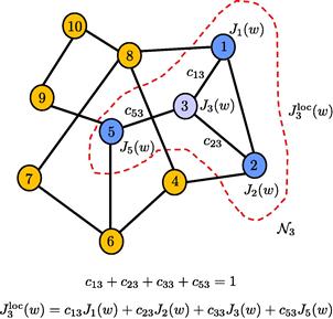
Figure 9.9 A network with ![]() nodes. The nodes in the neighborhood of node 3 are highlighted with their individual cost functions, and with the combination weights
nodes. The nodes in the neighborhood of node 3 are highlighted with their individual cost functions, and with the combination weights ![]() along the connecting edges; there is also a combination weight associated with node 3 and is denoted by
along the connecting edges; there is also a combination weight associated with node 3 and is denoted by ![]() . The expression for the local cost function,
. The expression for the local cost function, ![]() , is also shown in the figure.
, is also shown in the figure.
Now note that we can express ![]() from (9.104) as follows:
from (9.104) as follows:
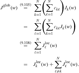 (9.113)
Substituting (9.110) into the second term on the right-hand side of the above expression gives:
![]() (9.114)
(9.114)
The last term in the above expression does not depend on ![]() . Therefore, minimizing
. Therefore, minimizing ![]() over
over ![]() is equivalent to minimizing the following alternative global cost:
is equivalent to minimizing the following alternative global cost:
![]() (9.115)
(9.115)
Expression (9.115) relates the optimization of the original global cost function, ![]() or its equivalent
or its equivalent ![]() , to the newly-introduced local cost function
, to the newly-introduced local cost function ![]() . The relation is through the second term on the right-hand side of (9.115), which corresponds to a sum of quadratic factors involving the minimizer
. The relation is through the second term on the right-hand side of (9.115), which corresponds to a sum of quadratic factors involving the minimizer ![]() ; this term tells us how the local cost
; this term tells us how the local cost ![]() can be corrected to the global cost
can be corrected to the global cost ![]() . Obviously, the minimizer
. Obviously, the minimizer ![]() that appears in the correction term is not known since the nodes wish to determine its value. Likewise, not all the weighting matrices
that appears in the correction term is not known since the nodes wish to determine its value. Likewise, not all the weighting matrices ![]() are available to node
are available to node ![]() ; only those matrices that originate from its neighbors can be assumed to be available. Still, expression (9.115) suggests a useful way to replace
; only those matrices that originate from its neighbors can be assumed to be available. Still, expression (9.115) suggests a useful way to replace ![]() by another local cost that is closer to
by another local cost that is closer to ![]() . This alternative cost will be shown to lead to a powerful distributed solution to optimize
. This alternative cost will be shown to lead to a powerful distributed solution to optimize ![]() through localized interactions.
through localized interactions.
Our first step is to limit the summation on the right-hand side of (9.115) to the neighbors of node ![]() (since every node
(since every node ![]() can only have access to information from its neighbors). We thus introduce the modified cost function at node
can only have access to information from its neighbors). We thus introduce the modified cost function at node ![]() :
:
![]() (9.116)
(9.116)
The cost functions ![]() and
and ![]() are both associated with node
are both associated with node ![]() ; the difference between them is that the expression for the latter is closer to the global cost function (9.115) that we want to optimize.
; the difference between them is that the expression for the latter is closer to the global cost function (9.115) that we want to optimize.
The weighting matrices ![]() that appear in (9.116) may or may not be available because the second-order moments
that appear in (9.116) may or may not be available because the second-order moments ![]() may or may not be known beforehand. If these moments are known, then we can proceed with the analysis by assuming knowledge of the
may or may not be known beforehand. If these moments are known, then we can proceed with the analysis by assuming knowledge of the ![]() . However, the more interesting case is when these moments are not known. This is generally the case in practice, especially in the context of adaptive solutions and problems involving non-stationary data. Often, nodes can only observe realizations
. However, the more interesting case is when these moments are not known. This is generally the case in practice, especially in the context of adaptive solutions and problems involving non-stationary data. Often, nodes can only observe realizations ![]() of the regression data
of the regression data ![]() arising from distributions whose covariance matrices are the unknown
arising from distributions whose covariance matrices are the unknown ![]() . One way to address the difficulty is to replace each of the weighted norms
. One way to address the difficulty is to replace each of the weighted norms ![]() in (9.116) by a scaled multiple of the un-weighted norm, say,
in (9.116) by a scaled multiple of the un-weighted norm, say,
![]() (9.117)
(9.117)
where ![]() is some nonnegative coefficient; we are even allowing its value to change with the node index
is some nonnegative coefficient; we are even allowing its value to change with the node index ![]() . The above substitution amounts to having each node
. The above substitution amounts to having each node ![]() approximate the
approximate the ![]() from its neighbors by multiples of the identity matrix
from its neighbors by multiples of the identity matrix
![]() (9.118)
(9.118)
Approximation (9.117) is reasonable in view of the fact that all vector norms are equivalent [19–21]; this norm property ensures that we can bound the weighted norm ![]() by some constants multiplying the un-weighted norm
by some constants multiplying the un-weighted norm ![]() say, as:
say, as:
![]() (9.119)
(9.119)
for some positive constants ![]() . Using the fact that the
. Using the fact that the ![]() are Hermitian positive-definite matrices, and calling upon the Rayleigh-Ritz characterization of eigenvalues [19,20], we can be more specific and replace the above inequalities by
are Hermitian positive-definite matrices, and calling upon the Rayleigh-Ritz characterization of eigenvalues [19,20], we can be more specific and replace the above inequalities by
![]() (9.120)
(9.120)
We note that approximations similar to (9.118) are common in stochastic approximation theory and they mark the difference between using a Newton’s iterative method or a stochastic gradient method [5,22]; the former uses Hessian matrices as approximations for ![]() and the latter uses multiples of the identity matrix. Furthermore, as the derivation will reveal, we do not need to worry at this stage about how to select the scalars
and the latter uses multiples of the identity matrix. Furthermore, as the derivation will reveal, we do not need to worry at this stage about how to select the scalars ![]() ; they will end up being embedded into another set of coefficients
; they will end up being embedded into another set of coefficients ![]() that will be set by the designer or adjusted by the algorithm—see (9.132) further ahead.
that will be set by the designer or adjusted by the algorithm—see (9.132) further ahead.
Thus, we replace (9.116) by
![]() (9.121)
(9.121)
The argument so far has suggested how to modify ![]() from (9.108) and replace it by the cost (9.121) that is closer in form to the global cost function (9.115). If we replace
from (9.108) and replace it by the cost (9.121) that is closer in form to the global cost function (9.115). If we replace ![]() by its definition (9.108), we can rewrite (9.121) as
by its definition (9.108), we can rewrite (9.121) as
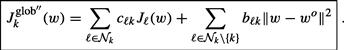 (9.122)
With the exception of the variable ![]() , this approximate cost at node
, this approximate cost at node ![]() relies solely on information that is available to node
relies solely on information that is available to node ![]() from its neighborhood. We will soon explain how to handle the fact that
from its neighborhood. We will soon explain how to handle the fact that ![]() is not known beforehand to node
is not known beforehand to node ![]() .
.
3.09.3.2 Steepest-descent iterations
Node ![]() can apply a steepest-descent iteration to minimize
can apply a steepest-descent iteration to minimize ![]() . Let
. Let ![]() denote the estimate for the minimizer
denote the estimate for the minimizer ![]() that is evaluated by node
that is evaluated by node ![]() at time
at time ![]() . Starting from an initial condition
. Starting from an initial condition ![]() , node
, node ![]() can compute successive estimates iteratively as follows:
can compute successive estimates iteratively as follows:
![]() (9.123)
(9.123)
where ![]() is a small positive step-size parameter, and the notation
is a small positive step-size parameter, and the notation ![]() denotes the gradient vector of the function
denotes the gradient vector of the function ![]() relative to
relative to ![]() and evaluated at
and evaluated at ![]() . The step-size parameter
. The step-size parameter ![]() can be selected to vary with time as well. One choice that is common in the optimization literature [5,22,23] is to replace
can be selected to vary with time as well. One choice that is common in the optimization literature [5,22,23] is to replace ![]() in (9.123) by step-size sequences
in (9.123) by step-size sequences ![]() that satisfy the two conditions (9.25). However, such step-size sequences are not suitable for applications that require continuous learning because they turn off adaptation as
that satisfy the two conditions (9.25). However, such step-size sequences are not suitable for applications that require continuous learning because they turn off adaptation as ![]() ; the steepest-descent iteration (9.123) would stop updating since
; the steepest-descent iteration (9.123) would stop updating since ![]() would be tending towards zero. For this reason, we shall focus mainly on the constant step-size case described by (9.123) since we are interested in developing distributed algorithms that will endow networks with continuous adaptation abilities.
would be tending towards zero. For this reason, we shall focus mainly on the constant step-size case described by (9.123) since we are interested in developing distributed algorithms that will endow networks with continuous adaptation abilities.
Returning to (9.123) and computing the gradient vector of (9.122) we get:
![]() (9.124)
(9.124)
Using the expression for ![]() from (9.97) we arrive at
from (9.97) we arrive at
![]() (9.125)
(9.125)
This iteration indicates that the update from ![]() to
to ![]() involves adding two correction terms to
involves adding two correction terms to ![]() . Among many other forms, we can implement the update in two successive steps by adding one correction term at a time, say, as follows:
. Among many other forms, we can implement the update in two successive steps by adding one correction term at a time, say, as follows:
![]() (9.126)
(9.126)
![]() (9.127)
(9.127)
Step (9.126) updates ![]() to an intermediate value
to an intermediate value ![]() by using local gradient vectors from the neighborhood of node
by using local gradient vectors from the neighborhood of node ![]() . Step (9.127) further updates
. Step (9.127) further updates ![]() to
to ![]() . Two issues stand out from examining (9.127):
. Two issues stand out from examining (9.127):
a. First, iteration (9.127) requires knowledge of the minimizer ![]() . Neither node
. Neither node ![]() nor its neighbors know the value of the minimizer; each of these nodes is actually performing steps similar to (9.126) and (9.127) to estimate the minimizer. However, each node
nor its neighbors know the value of the minimizer; each of these nodes is actually performing steps similar to (9.126) and (9.127) to estimate the minimizer. However, each node ![]() has a readily available approximation for
has a readily available approximation for ![]() , which is its local intermediate estimate
, which is its local intermediate estimate ![]() . Therefore, we replace
. Therefore, we replace ![]() in (9.127) by
in (9.127) by ![]() . This step helps diffuse information throughout the network. This is because each neighbor of node
. This step helps diffuse information throughout the network. This is because each neighbor of node ![]() determines its estimate
determines its estimate ![]() by processing information from its own neighbors, which process information from their neighbors, and so forth.
by processing information from its own neighbors, which process information from their neighbors, and so forth.
b. Second, the intermediate value ![]() at node
at node ![]() is generally a better estimate for
is generally a better estimate for ![]() than
than ![]() since it is obtained by incorporating information from the neighbors through the first step (9.126). Therefore, we further replace
since it is obtained by incorporating information from the neighbors through the first step (9.126). Therefore, we further replace ![]() in (9.127) by
in (9.127) by ![]() . This step is reminiscent of incremental-type approaches to optimization, which have been widely studied in the literature [24–27].
. This step is reminiscent of incremental-type approaches to optimization, which have been widely studied in the literature [24–27].
With the substitutions described in items (a) and (b) above, we replace the second step (9.127) by
 (9.128)
Introduce the weighting coefficients:
![]() (9.129)
(9.129)
![]() (9.130)
(9.130)
![]() (9.131)
(9.131)
and observe that, for sufficiently small step-sizes ![]() , these coefficients are nonnegative and, moreover, they satisfy the conditions:
, these coefficients are nonnegative and, moreover, they satisfy the conditions:
 (9.132)
Condition (9.132) means that for every node ![]() , the sum of the coefficients
, the sum of the coefficients ![]() that relate it to its neighbors is one. Just like the
that relate it to its neighbors is one. Just like the ![]() , from now on, we will treat the coefficients
, from now on, we will treat the coefficients ![]() as free weighting parameters that are chosen by the designer according to (9.132); their selection will also have a bearing on the performance of the resulting algorithms—see Theorem 9.6.8. If we collect the entries
as free weighting parameters that are chosen by the designer according to (9.132); their selection will also have a bearing on the performance of the resulting algorithms—see Theorem 9.6.8. If we collect the entries ![]() into an
into an ![]() matrix
matrix ![]() , such that the
, such that the ![]() th column of
th column of ![]() consists of
consists of ![]() , then condition (9.132) translates into saying that each column of
, then condition (9.132) translates into saying that each column of ![]() adds up to one:
adds up to one:
![]() (9.133)
(9.133)
We say that ![]() is a left stochastic matrix.
is a left stochastic matrix.
3.09.3.3 Adapt-then-Combine (ATC) diffusion strategy
Using the coefficients ![]() so defined, we replace (9.126) and (9.128) by the following recursions for
so defined, we replace (9.126) and (9.128) by the following recursions for ![]() :
:
 (9.134)
for some nonnegative coefficients ![]() that satisfy conditions (9.106) and (9.133), namely,
that satisfy conditions (9.106) and (9.133), namely,
![]() (9.135)
(9.135)
or, equivalently,
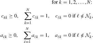 (9.136)
To run algorithm (9.134), we only need to select the coefficients ![]() that satisfy (9.135) or (9.136); there is no need to worry about the intermediate coefficients
that satisfy (9.135) or (9.136); there is no need to worry about the intermediate coefficients ![]() any longer since they have been blended into the
any longer since they have been blended into the ![]() . The scalars
. The scalars ![]() that appear in (9.134) correspond to weighting coefficients over the edge linking node
that appear in (9.134) correspond to weighting coefficients over the edge linking node ![]() to its neighbors
to its neighbors ![]() . Note that two sets of coefficients are used to scale the data that are being received by node
. Note that two sets of coefficients are used to scale the data that are being received by node ![]() : one set of coefficients,
: one set of coefficients, ![]() is used in the first step of (9.134) to scale the moment data
is used in the first step of (9.134) to scale the moment data ![]() , and a second set of coefficients,
, and a second set of coefficients, ![]() is used in the second step of (9.134) to scale the estimates
is used in the second step of (9.134) to scale the estimates ![]() . Figure 9.10 explains what the entries on the columns and rows of the combination matrices
. Figure 9.10 explains what the entries on the columns and rows of the combination matrices ![]() stand for using an example with
stand for using an example with ![]() and the matrix
and the matrix ![]() for illustration. When the combination matrix is right-stochastic (as is the case with
for illustration. When the combination matrix is right-stochastic (as is the case with ![]() ), each of its rows would add up to one. On the other hand, when the matrix is left-stochastic (as is the case with
), each of its rows would add up to one. On the other hand, when the matrix is left-stochastic (as is the case with ![]() ), each of its columns would add up to one.
), each of its columns would add up to one.

Figure 9.10 Interpretation of the columns and rows of combination matrices. The pair of entries ![]() correspond to weighting coefficients used over the edge connecting nodes
correspond to weighting coefficients used over the edge connecting nodes ![]() and
and ![]() . When nodes
. When nodes ![]() are not neighbors, then these weights are zero.
are not neighbors, then these weights are zero.
At every time instant ![]() , the ATC strategy (9.134) performs two steps. The first step is an information exchange step where node
, the ATC strategy (9.134) performs two steps. The first step is an information exchange step where node ![]() receives from its neighbors their moments
receives from its neighbors their moments ![]() . Node
. Node ![]() combines this information and uses it to update its existing estimate
combines this information and uses it to update its existing estimate ![]() to an intermediate value
to an intermediate value ![]() . All other nodes in the network are performing a similar step and updating their existing estimates
. All other nodes in the network are performing a similar step and updating their existing estimates ![]() into intermediate estimates
into intermediate estimates ![]() by using information from their neighbors. The second step in (9.134) is an aggregation or consultation step where node
by using information from their neighbors. The second step in (9.134) is an aggregation or consultation step where node ![]() combines the intermediate estimates of its neighbors to obtain its updated estimate
combines the intermediate estimates of its neighbors to obtain its updated estimate ![]() . Again, all other nodes in the network are simultaneously performing a similar step. The reason for the name Adapt-then-Combine (ATC) strategy is that the first step in (9.134) will be shown to lead to an adaptive step, while the second step in (9.134) corresponds to a combination step. Hence, strategy (9.134) involves adaptation followed by combination or ATC for short. The reason for the qualification “diffusion” is that the combination step in (9.134) allows information to diffuse through the network in real time. This is because each of the estimates
. Again, all other nodes in the network are simultaneously performing a similar step. The reason for the name Adapt-then-Combine (ATC) strategy is that the first step in (9.134) will be shown to lead to an adaptive step, while the second step in (9.134) corresponds to a combination step. Hence, strategy (9.134) involves adaptation followed by combination or ATC for short. The reason for the qualification “diffusion” is that the combination step in (9.134) allows information to diffuse through the network in real time. This is because each of the estimates ![]() is influenced by data beyond the immediate neighborhood of node
is influenced by data beyond the immediate neighborhood of node ![]() .
.
In the special case when ![]() , so that no information exchange is performed but only the aggregation step, the ATC strategy (9.134) reduces to:
, so that no information exchange is performed but only the aggregation step, the ATC strategy (9.134) reduces to:
 (9.137)
where the first step relies solely on the information ![]() that is available locally at node
that is available locally at node ![]() .
.
Observe in passing that the term that appears in the information exchange step of (9.134) is related to the gradient vectors of the local costs ![]() evaluated at
evaluated at ![]() , i.e., it holds that
, i.e., it holds that
![]() (9.138)
(9.138)
so that the ATC strategy (9.134) can also be written in the following equivalent form:
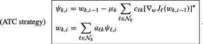 (9.139)
The significance of this general form is that it is applicable to optimization problems involving more general local costs ![]() that are not necessarily quadratic in
that are not necessarily quadratic in ![]() , as detailed in [1–3]—see also Section 3.09.10.4. The top part of Figure 9.11 illustrates the two steps involved in the ATC procedure for a situation where node
, as detailed in [1–3]—see also Section 3.09.10.4. The top part of Figure 9.11 illustrates the two steps involved in the ATC procedure for a situation where node ![]() has three other neighbors labeled
has three other neighbors labeled ![]() . In the first step, node
. In the first step, node ![]() evaluates the gradient vectors of its neighbors at
evaluates the gradient vectors of its neighbors at ![]() , and subsequently aggregates the estimates
, and subsequently aggregates the estimates ![]() from its neighbors. The dotted arrows represent flow of information towards node
from its neighbors. The dotted arrows represent flow of information towards node ![]() from its neighbors. The solid arrows represent flow of information from node
from its neighbors. The solid arrows represent flow of information from node ![]() to its neighbors. The CTA diffusion strategy is discussed next.
to its neighbors. The CTA diffusion strategy is discussed next.
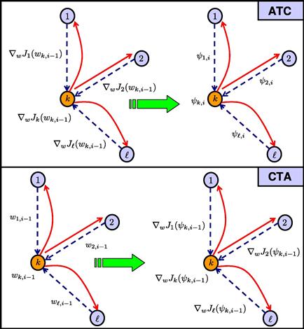
Figure 9.11 Illustration of the ATC and CTA strategies for a node ![]() with three other neighbors
with three other neighbors ![]() . The updates involve two steps: information exchange followed by aggregation in ATC and aggregation followed by information exchange in CTA. The dotted arrows represent the data received from the neighbors of node
. The updates involve two steps: information exchange followed by aggregation in ATC and aggregation followed by information exchange in CTA. The dotted arrows represent the data received from the neighbors of node ![]() , and the solid arrows represent the data sent from node
, and the solid arrows represent the data sent from node ![]() to its neighbors.
to its neighbors.
3.09.3.4 Combine-then-Adapt (CTA) diffusion strategy
Similarly, if we return to (9.125) and add the second correction term first, then (9.126) and (9.127) are replaced by:
![]() (9.140)
(9.140)
![]() (9.141)
(9.141)
Following similar reasoning to what we did before in the ATC case, we replace ![]() in step (9.140) by
in step (9.140) by ![]() and replace
and replace ![]() in (9.141) by
in (9.141) by ![]() . We then introduce the same coefficients
. We then introduce the same coefficients ![]() and arrive at the following Combine-then-Adapt (CTA) strategy:
and arrive at the following Combine-then-Adapt (CTA) strategy:
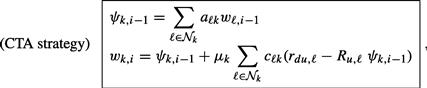 (9.142)
where the nonnegative coefficients ![]() satisfy the same conditions (9.106) and (9.133), namely,
satisfy the same conditions (9.106) and (9.133), namely,
![]() (9.143)
(9.143)
 (9.144)
At every time instant ![]() , the CTA strategy (9.142) also consists of two steps. The first step is an aggregation step where node
, the CTA strategy (9.142) also consists of two steps. The first step is an aggregation step where node ![]() combines the existing estimates of its neighbors to obtain the intermediate estimate
combines the existing estimates of its neighbors to obtain the intermediate estimate ![]() . All other nodes in the network are simultaneously performing a similar step and aggregating the estimates of their neighbors. The second step in (9.142) is an information exchange step where node
. All other nodes in the network are simultaneously performing a similar step and aggregating the estimates of their neighbors. The second step in (9.142) is an information exchange step where node ![]() receives from its neighbors their moments
receives from its neighbors their moments ![]() and uses this information to update its intermediate estimate to
and uses this information to update its intermediate estimate to ![]() . Again, all other nodes in the network are simultaneously performing a similar information exchange step. The reason for the name Combine-then-Adapt (CTA) strategy is that the first step in (9.142) involves a combination step, while the second step will be shown to lead to an adaptive step. Hence, strategy (9.142) involves combination followed by adaptation or CTA for short. The reason for the qualification “diffusion” is that the combination step of (9.142) allows information to diffuse through the network in real time.
. Again, all other nodes in the network are simultaneously performing a similar information exchange step. The reason for the name Combine-then-Adapt (CTA) strategy is that the first step in (9.142) involves a combination step, while the second step will be shown to lead to an adaptive step. Hence, strategy (9.142) involves combination followed by adaptation or CTA for short. The reason for the qualification “diffusion” is that the combination step of (9.142) allows information to diffuse through the network in real time.
In the special case when ![]() , so that no information exchange is performed but only the aggregation step, the CTA strategy (9.142) reduces to:
, so that no information exchange is performed but only the aggregation step, the CTA strategy (9.142) reduces to:
 (9.145)
where the second step relies solely on the information ![]() that is available locally at node
that is available locally at node ![]() . Again, the CTA strategy (9.142) can be rewritten in terms of the gradient vectors of the local costs
. Again, the CTA strategy (9.142) can be rewritten in terms of the gradient vectors of the local costs ![]() as follows:
as follows:
 (9.146)
The bottom part of Figure 9.11 illustrates the two steps involved in the CTA procedure for a situation where node ![]() has three other neighbors labeled
has three other neighbors labeled ![]() . In the first step, node
. In the first step, node ![]() aggregates the estimates
aggregates the estimates ![]() from its neighbors, and subsequently performs information exchange by evaluating the gradient vectors of its neighbors at
from its neighbors, and subsequently performs information exchange by evaluating the gradient vectors of its neighbors at ![]() .
.
3.09.3.5 Useful properties of diffusion strategies
Note that the structure of the ATC and CTA diffusion strategies (9.134) and (9.142) are fundamentally the same: the difference between the implementations lies in which variable we choose to correspond to the updated weight estimate ![]() . In the ATC case, we choose the result of the combination step to be
. In the ATC case, we choose the result of the combination step to be ![]() , whereas in the CTA case we choose the result of the adaptation step to be
, whereas in the CTA case we choose the result of the adaptation step to be ![]() .
.
For ease of reference, Table 9.2 lists the steepest-descent diffusion algorithms derived in the previous sections. The derivation of the ATC and CTA strategies (9.134) and (9.142) followed the approach proposed in [18,28]. CTA estimation schemes were first proposed in the works [29–33], and later extended in [18,28,34,35]. The earlier versions of CTA in [29–31] used the choice ![]() . This form of the algorithm with
. This form of the algorithm with ![]() , and with the additional constraint that the step-sizes
, and with the additional constraint that the step-sizes ![]() should be time-dependent and decay towards zero as time progresses, was later applied by [36,37] to solve distributed optimization problems that require all nodes to reach consensus or agreement. Likewise, special cases of the ATC estimation scheme (9.134), involving an information exchange step followed by an aggregation step, first appeared in the work [38] on diffusion least-squares schemes and subsequently in the works [18,34,35,39–41] on distributed mean-square-error and state-space estimation methods. A special case of the ATC strategy (9.134) corresponding to the choice
should be time-dependent and decay towards zero as time progresses, was later applied by [36,37] to solve distributed optimization problems that require all nodes to reach consensus or agreement. Likewise, special cases of the ATC estimation scheme (9.134), involving an information exchange step followed by an aggregation step, first appeared in the work [38] on diffusion least-squares schemes and subsequently in the works [18,34,35,39–41] on distributed mean-square-error and state-space estimation methods. A special case of the ATC strategy (9.134) corresponding to the choice ![]() with decaying step-sizes was adopted in [42] to ensure convergence towards a consensus state. Diffusion strategies of the form (9.134) and (9.142) (or, equivalently, (9.139) and (9.146)) are general in several respects:
with decaying step-sizes was adopted in [42] to ensure convergence towards a consensus state. Diffusion strategies of the form (9.134) and (9.142) (or, equivalently, (9.139) and (9.146)) are general in several respects:
1. These strategies do not only diffuse the local weight estimates, but they can also diffuse the local gradient vectors. In other words, two sets of combination coefficients ![]() can be used.
can be used.
2. In the derivation that led to the diffusion strategies, the combination matrices ![]() and
and ![]() are only required to be right-stochastic (for
are only required to be right-stochastic (for ![]() ) and left-stochastic (for
) and left-stochastic (for ![]() ). In comparison, it is common in consensus-type strategies to require the corresponding combination matrix
). In comparison, it is common in consensus-type strategies to require the corresponding combination matrix ![]() to be doubly stochastic (i.e., its rows and columns should add up to one)—see, e.g., Appendix E and [36,43–45].
to be doubly stochastic (i.e., its rows and columns should add up to one)—see, e.g., Appendix E and [36,43–45].
3. As the analysis in Section 3.09.6 will reveal, ATC and CTA strategies do not force nodes to converge to an agreement about the desired parameter vector ![]() , as is common in consensus-type strategies (see Appendix E and [36,46–52]). Forcing nodes to reach agreement on
, as is common in consensus-type strategies (see Appendix E and [36,46–52]). Forcing nodes to reach agreement on ![]() ends up limiting the adaptation and learning abilities of these nodes, as well as their ability to react to information in real-time. Nodes in diffusion networks enjoy more flexibility in the learning process, which allows their individual estimates,
ends up limiting the adaptation and learning abilities of these nodes, as well as their ability to react to information in real-time. Nodes in diffusion networks enjoy more flexibility in the learning process, which allows their individual estimates, ![]() , to tend to values that lie within a reasonable mean-square-deviation (MSD) level from the optimal solution,
, to tend to values that lie within a reasonable mean-square-deviation (MSD) level from the optimal solution, ![]() . Multi-agent systems in nature behave in this manner; they do not require exact agreement among their agents (see, e.g., [8–10]).
. Multi-agent systems in nature behave in this manner; they do not require exact agreement among their agents (see, e.g., [8–10]).
4. The step-size parameters ![]() are not required to depend on the time index
are not required to depend on the time index ![]() and are not required to vanish as
and are not required to vanish as ![]() (as is common in many works on distributed optimization, e.g., [22,23,36,53]). Instead, the step-sizes can assume constant values, which is a critical property to endow networks with continuous adaptation and learning abilities. An important contribution in the study of diffusion strategies is to show that distributed optimization is still possible even for constant step-sizes, in addition to the ability to perform adaptation, learning, and tracking. Sections 3.09.5 and 3.09.6 highlight the convergence properties of the diffusion strategies—see also [1–3] for results pertaining to more general cost functions.
(as is common in many works on distributed optimization, e.g., [22,23,36,53]). Instead, the step-sizes can assume constant values, which is a critical property to endow networks with continuous adaptation and learning abilities. An important contribution in the study of diffusion strategies is to show that distributed optimization is still possible even for constant step-sizes, in addition to the ability to perform adaptation, learning, and tracking. Sections 3.09.5 and 3.09.6 highlight the convergence properties of the diffusion strategies—see also [1–3] for results pertaining to more general cost functions.
5. Even the combination weights ![]() can be adapted, as we shall discuss later in Section 3.09.8.3. In this way, diffusion strategies allow multiple layers of adaptation: the nodes perform adaptive processing, the combination weights can be adapted, and even the topology can be adapted especially for mobile networks [8].
can be adapted, as we shall discuss later in Section 3.09.8.3. In this way, diffusion strategies allow multiple layers of adaptation: the nodes perform adaptive processing, the combination weights can be adapted, and even the topology can be adapted especially for mobile networks [8].
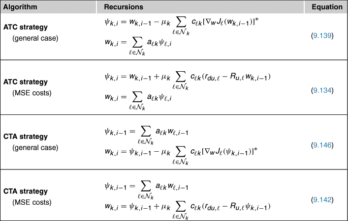
3.09.4 Adaptive diffusion strategies
The distributed ATC and CTA steepest-descent strategies (9.134) and (9.142) for determining the ![]() that solves (9.92) and (9.93) require knowledge of the statistical information
that solves (9.92) and (9.93) require knowledge of the statistical information ![]() . These moments are needed in order to be able to evaluate the gradient vectors that appear in (9.134) and (9.142), namely, the terms:
. These moments are needed in order to be able to evaluate the gradient vectors that appear in (9.134) and (9.142), namely, the terms:
![]() (9.147)
(9.147)
![]() (9.148)
(9.148)
for all ![]() . However, the moments
. However, the moments ![]() are often not available beforehand, which means that the true gradient vectors are generally not available. Instead, the agents have access to observations
are often not available beforehand, which means that the true gradient vectors are generally not available. Instead, the agents have access to observations ![]() of the random processes
of the random processes ![]() . There are many ways by which the true gradient vectors can be approximated by using these observations. Recall that, by definition,
. There are many ways by which the true gradient vectors can be approximated by using these observations. Recall that, by definition,
![]() (9.149)
(9.149)
One common stochastic approximation method is to drop the expectation operator from the definitions of ![]() and to use the following instantaneous approximations instead [4–7]:
and to use the following instantaneous approximations instead [4–7]:
![]() (9.150)
(9.150)
In this case, the approximate gradient vectors become:
![]() (9.151)
(9.151)
![]() (9.152)
(9.152)
Substituting into the ATC and CTA steepest-descent strategies (9.134) and (9.142), we arrive at the following adaptive implementations of the diffusion strategies for ![]() :
:
 (9.153)
and
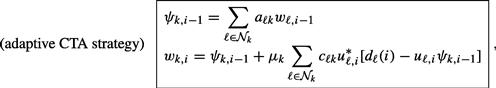 (9.154)
where the coefficients ![]() are chosen to satisfy:
are chosen to satisfy:
 (9.155)
The adaptive implementations usually start from the initial conditions ![]() for all
for all ![]() , or from some other convenient initial values. Clearly, in view of the approximations (9.151) and (9.152), the successive iterates
, or from some other convenient initial values. Clearly, in view of the approximations (9.151) and (9.152), the successive iterates ![]() that are generated by the above adaptive implementations are different from the iterates that result from the steepest-descent implementations (9.134) and (9.142). Nevertheless, we shall continue to use the same notation for these variables for ease of reference. One key advantage of the adaptive implementations (9.153) and (9.154) are that they enable the agents to react to changes in the underlying statistical information
that are generated by the above adaptive implementations are different from the iterates that result from the steepest-descent implementations (9.134) and (9.142). Nevertheless, we shall continue to use the same notation for these variables for ease of reference. One key advantage of the adaptive implementations (9.153) and (9.154) are that they enable the agents to react to changes in the underlying statistical information ![]() and to changes in
and to changes in ![]() . This is because these changes end up being reflected in the data realizations
. This is because these changes end up being reflected in the data realizations ![]() . Therefore, adaptive implementations have an innate tracking and learning ability that is of paramount significance in practice.
. Therefore, adaptive implementations have an innate tracking and learning ability that is of paramount significance in practice.
We say that the stochastic gradient approximations (9.151) and (9.152) introduce gradient noise into each step of the recursive updates (9.153) and (9.154). This is because the updates (9.153) and (9.154) can be interpreted as corresponding to the following forms:
 (9.156)
and
 (9.157)
where the true gradient vectors, ![]() , have been replaced by approximations,
, have been replaced by approximations, ![]() —compare with (9.139) and (9.146). The significance of the alternative forms (9.156) and (9.157) is that they are applicable to optimization problems involving more general local costs
—compare with (9.139) and (9.146). The significance of the alternative forms (9.156) and (9.157) is that they are applicable to optimization problems involving more general local costs ![]() that are not necessarily quadratic, as detailed in [1–3]; see also Section 3.09.10.4. In the next section, we examine how gradient noise affects the performance of the diffusion strategies and how close the successive estimates
that are not necessarily quadratic, as detailed in [1–3]; see also Section 3.09.10.4. In the next section, we examine how gradient noise affects the performance of the diffusion strategies and how close the successive estimates ![]() get to the desired optimal solution
get to the desired optimal solution ![]() . Table 9.3 lists several of the adaptive diffusion algorithms derived in this section.
. Table 9.3 lists several of the adaptive diffusion algorithms derived in this section.
Table 9.3
Summary of Adaptive Diffusion Strategies for the Distributed Optimization of Problems of the form (9.92), and their Specialization to the Case of Mean- Square-Error (MSE) Individual Cost Functions Given by (9.93). These Adaptive Solutions Rely on Stochastic Approximations
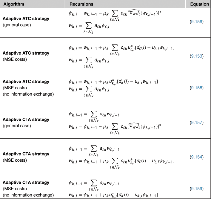
The operation of the adaptive diffusion strategies is similar to the operation of the steepest-descent diffusion strategies of the previous section. Thus, note that at every time instant ![]() , the ATC strategy (9.153) performs two steps; as illustrated in Figure 9.12. The first step is an information exchange step where node
, the ATC strategy (9.153) performs two steps; as illustrated in Figure 9.12. The first step is an information exchange step where node ![]() receives from its neighbors their information
receives from its neighbors their information ![]() . Node
. Node ![]() combines this information and uses it to update its existing estimate
combines this information and uses it to update its existing estimate ![]() to an intermediate value
to an intermediate value ![]() . All other nodes in the network are performing a similar step and updating their existing estimates
. All other nodes in the network are performing a similar step and updating their existing estimates ![]() into intermediate estimates
into intermediate estimates ![]() by using information from their neighbors. The second step in (9.153) is an aggregation or consultation step where node
by using information from their neighbors. The second step in (9.153) is an aggregation or consultation step where node ![]() combines the intermediate estimates
combines the intermediate estimates ![]() of its neighbors to obtain its updated estimate
of its neighbors to obtain its updated estimate ![]() . Again, all other nodes in the network are simultaneously performing a similar step. In the special case when
. Again, all other nodes in the network are simultaneously performing a similar step. In the special case when ![]() , so that no information exchange is performed but only the aggregation step, the ATC strategy (9.153) reduces to:
, so that no information exchange is performed but only the aggregation step, the ATC strategy (9.153) reduces to:
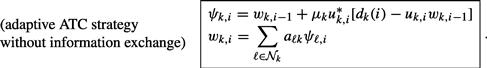 (9.158)

Figure 9.12 Illustration of the adaptive ATC strategy, which involves two steps: information exchange followed by aggregation.
Likewise, at every time instant ![]() , the CTA strategy (9.154) also consists of two steps—see Figure 9.13. The first step is an aggregation step where node
, the CTA strategy (9.154) also consists of two steps—see Figure 9.13. The first step is an aggregation step where node ![]() combines the existing estimates of its neighbors to obtain the intermediate estimate
combines the existing estimates of its neighbors to obtain the intermediate estimate ![]() . All other nodes in the network are simultaneously performing a similar step and aggregating the estimates of their neighbors. The second step in (9.154) is an information exchange step where node
. All other nodes in the network are simultaneously performing a similar step and aggregating the estimates of their neighbors. The second step in (9.154) is an information exchange step where node ![]() receives from its neighbors their information
receives from its neighbors their information ![]() and uses this information to update its intermediate estimate to
and uses this information to update its intermediate estimate to ![]() . Again, all other nodes in the network are simultaneously performing a similar information exchange step. In the special case when
. Again, all other nodes in the network are simultaneously performing a similar information exchange step. In the special case when ![]() , so that no information exchange is performed but only the aggregation step, the CTA strategy (9.154) reduces to:
, so that no information exchange is performed but only the aggregation step, the CTA strategy (9.154) reduces to:
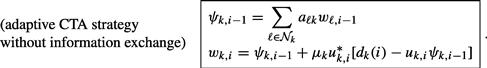 (9.159)

Figure 9.13 Illustration of the adaptive CTA strategy, which involves two steps: aggregation followed by information exchange.
We further note that the adaptive ATC and CTA strategies (9.153) and (9.154) reduce to the non-cooperative adaptive solution (9.22) and (9.23), where each node k runs its own individual LMS filter, when the coefficients ![]() are selected as
are selected as
![]() (9.160)
(9.160)
where ![]() denotes the Kronecker delta function:
denotes the Kronecker delta function:
 (9.161)
In terms of the combination matrices ![]() and
and ![]() , this situation corresponds to setting
, this situation corresponds to setting
![]() (9.162)
(9.162)
3.09.5 Performance of steepest-descent diffusion strategies
Before studying in some detail the mean-square performance of the adaptive diffusion implementations (9.153) and (9.154), and the influence of gradient noise, we examine first the convergence behavior of the steepest-descent diffusion strategies (9.134) and (9.142), which employ the true gradient vectors. Doing so will help introduce the necessary notation and highlight some features of the analysis in preparation for the more challenging treatment of the adaptive strategies in Section 3.09.6.
3.09.5.1 General diffusion model
Rather than study the performance of the ATC and CTA steepest-descent strategies (9.134) and (9.142) separately, it is useful to introduce a more general description that includes the ATC and CTA recursions as special cases. Thus, consider a distributed steepest-descent diffusion implementation of the following general form for ![]() :
:
![]() (9.163)
(9.163)
![]() (9.164)
(9.164)
![]() (9.165)
(9.165)
where the scalars ![]() denote three sets of nonnegative real coefficients corresponding to the
denote three sets of nonnegative real coefficients corresponding to the ![]() entries of
entries of ![]() combination matrices
combination matrices ![]() , respectively. These matrices are assumed to satisfy the conditions:
, respectively. These matrices are assumed to satisfy the conditions:
![]() (9.166)
(9.166)
so that ![]() are left stochastic and
are left stochastic and ![]() is right-stochastic, i.e.,
is right-stochastic, i.e.,
 (9.167)
As indicated in Table 9.4, different choices for ![]() correspond to different cooperation modes. For example, the choice
correspond to different cooperation modes. For example, the choice ![]() and
and ![]() corresponds to the ATC implementation (9.134), while the choice
corresponds to the ATC implementation (9.134), while the choice ![]() and
and ![]() corresponds to the CTA implementation (9.142). Likewise, the choice
corresponds to the CTA implementation (9.142). Likewise, the choice ![]() corresponds to the case in which the nodes only share weight estimates and the distributed diffusion recursions (9.163) to (9.165) become:
corresponds to the case in which the nodes only share weight estimates and the distributed diffusion recursions (9.163) to (9.165) become:
![]() (9.168)
(9.168)
![]() (9.169)
(9.169)
![]() (9.170)
(9.170)
Furthermore, the choice ![]() corresponds to the non-cooperative mode of operation, in which case the recursions reduce to the classical (stand-alone) steepest-descent recursion [4–7], where each node minimizes individually its own quadratic cost
corresponds to the non-cooperative mode of operation, in which case the recursions reduce to the classical (stand-alone) steepest-descent recursion [4–7], where each node minimizes individually its own quadratic cost ![]() , defined earlier in (9.97):
, defined earlier in (9.97):
![]() (9.171)
(9.171)
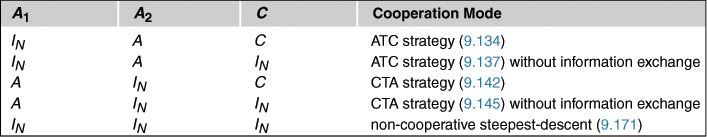
3.09.5.2 Error recursions
Our objective is to examine whether, and how fast, the weight estimates ![]() from the distributed implementation (9.163)–(9.165) converge towards the solution
from the distributed implementation (9.163)–(9.165) converge towards the solution ![]() of (9.92) and (9.93). To do so, we introduce the
of (9.92) and (9.93). To do so, we introduce the ![]() error vectors:
error vectors:
![]() (9.172)
(9.172)
![]() (9.173)
(9.173)
![]() (9.174)
(9.174)
Each of these error vectors measures the residual relative to the desired minimizer ![]() . Now recall from (9.100) that
. Now recall from (9.100) that
![]() (9.175)
(9.175)
Then, subtracting ![]() from both sides of relations in (9.163)–(9.165) we get
from both sides of relations in (9.163)–(9.165) we get
![]() (9.176)
(9.176)
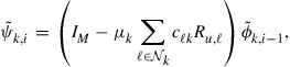 (9.177)
![]() (9.178)
(9.178)
We can describe these relations more compactly by collecting the information from across the network into block vectors and matrices. We collect the error vectors from across all nodes into the following ![]() block vectors, whose individual entries are of size
block vectors, whose individual entries are of size ![]() each:
each:
 (9.179)
The block quantities ![]() represent the state of the errors across the network at time
represent the state of the errors across the network at time ![]() . Likewise, we introduce the following
. Likewise, we introduce the following ![]() block diagonal matrices, whose individual entries are of size
block diagonal matrices, whose individual entries are of size ![]() each:
each:
![]() (9.180)
(9.180)
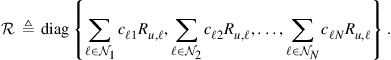 (9.181)
Each block diagonal entry of ![]() , say, the
, say, the ![]() th entry, contains the combination of the covariance matrices in the neighborhood of node
th entry, contains the combination of the covariance matrices in the neighborhood of node ![]() . We can simplify the notation by denoting these neighborhood combinations as follows:
. We can simplify the notation by denoting these neighborhood combinations as follows:
![]() (9.182)
(9.182)
so that ![]() becomes
becomes
![]() (9.183)
(9.183)
In the special case when ![]() , the matrix
, the matrix ![]() reduces to
reduces to
![]() (9.184)
(9.184)
with the individual covariance matrices appearing on its diagonal; we denote ![]() by
by ![]() in this special case. We further introduce the Kronecker products
in this special case. We further introduce the Kronecker products
![]() (9.185)
(9.185)
The matrix ![]() is an
is an ![]() block matrix whose
block matrix whose ![]() block is equal to
block is equal to ![]() . Likewise, for
. Likewise, for ![]() . In other words, the Kronecker transformation defined above simply replaces the matrices
. In other words, the Kronecker transformation defined above simply replaces the matrices ![]() by block matrices
by block matrices ![]() where each entry
where each entry ![]() in the original matrices is replaced by the diagonal matrices
in the original matrices is replaced by the diagonal matrices ![]() . For ease of reference, Table 9.5 lists the various symbols that have been defined so far, and others that will be defined in the sequel.
. For ease of reference, Table 9.5 lists the various symbols that have been defined so far, and others that will be defined in the sequel.
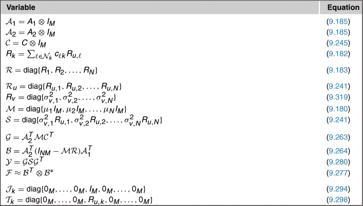
Returning to (9.176)–(9.178), we conclude that the following relations hold for the block quantities:
![]() (9.186)
(9.186)
![]() (9.187)
(9.187)
![]() (9.188)
(9.188)
so that the network weight error vector, ![]() , ends up evolving according to the following dynamics:
, ends up evolving according to the following dynamics:
![]() (9.189)
(9.189)
For comparison purposes, if each node in the network minimizes its own cost function, ![]() , separately from the other nodes and uses the non-cooperative steepest-descent strategy (9.171), then the weight error vector across all
, separately from the other nodes and uses the non-cooperative steepest-descent strategy (9.171), then the weight error vector across all ![]() nodes would evolve according to the following alternative dynamics:
nodes would evolve according to the following alternative dynamics:
![]() (9.190)
(9.190)
where the matrices ![]() and
and ![]() do not appear, and
do not appear, and ![]() is replaced by
is replaced by ![]() from (9.184). This recursion is a special case of (9.189) when
from (9.184). This recursion is a special case of (9.189) when ![]() .
.
3.09.5.3 Convergence behavior
Note from (9.189) that the evolution of the weight error vector involves block vectors and block matrices; this will be characteristic of the distributed implementations that we consider in this chapter. To examine the stability and convergence properties of recursions that involve such block quantities, it becomes useful to rely on a certain block vector norm. In Appendix D, we describe a so-called block maximum norm and establish some of its useful properties. The results of the appendix will be used extensively in our exposition. It is therefore advisable for the reader to review the properties stated in the appendix at this stage.
Using the result of Lemma D.6, we can establish the following useful statement about the convergence of the steepest-descent diffusion strategy (9.163)–(9.165). The result establishes that all nodes end up converging to the optimal solution ![]() if the nodes employ positive step-sizes
if the nodes employ positive step-sizes ![]() that are small enough; the lemma provides a sufficient bound on the
that are small enough; the lemma provides a sufficient bound on the ![]() .
.
Theorem 9.5.1
Convergence to Optimal Solution
Consider the problem of optimizing the global cost (9.92) with the individual cost functions given by (9.93). Pick a right stochastic matrix ![]() and left stochastic matrices
and left stochastic matrices ![]() and
and ![]() satisfying (9.166) or (9.167); these matrices define the network topology and how information is shared over neighborhoods. Assume each node in the network runs the (distributed) steepest-descent diffusion algorithm (9.163)–(9.165). Then, all estimates
satisfying (9.166) or (9.167); these matrices define the network topology and how information is shared over neighborhoods. Assume each node in the network runs the (distributed) steepest-descent diffusion algorithm (9.163)–(9.165). Then, all estimates ![]() across the network converge to the optimal solution
across the network converge to the optimal solution ![]() if the positive step-size parameters
if the positive step-size parameters ![]() satisfy
satisfy
![]() (9.191)
(9.191)
where the neighborhood covariance matrix ![]() is defined by (9.182).
is defined by (9.182).
Proof.
The weight error vector ![]() converges to zero if, and only if, the coefficient matrix
converges to zero if, and only if, the coefficient matrix ![]() in (9.189) is a stable matrix (meaning that all its eigenvalues lie strictly inside the unit disc). From property (9.605) established in Appendix D, we know that
in (9.189) is a stable matrix (meaning that all its eigenvalues lie strictly inside the unit disc). From property (9.605) established in Appendix D, we know that ![]() is stable if the block diagonal matrix
is stable if the block diagonal matrix ![]() is stable. It is now straightforward to verify that condition (9.191) ensures the stability of
is stable. It is now straightforward to verify that condition (9.191) ensures the stability of ![]() . It follows that
. It follows that
![]() (9.192)
(9.192)
![]()
Observe that the stability condition (9.191) does not depend on the specific combination matrices ![]() and
and ![]() . Thus, as long as these matrices are chosen to be left-stochastic, the weight-error vectors will converge to zero under condition (9.191) no matter what
. Thus, as long as these matrices are chosen to be left-stochastic, the weight-error vectors will converge to zero under condition (9.191) no matter what ![]() are. Only the combination matrix
are. Only the combination matrix ![]() influences the condition on the step-size through the neighborhood covariance matrices
influences the condition on the step-size through the neighborhood covariance matrices ![]() . Observe further that the statement of the lemma does not require the network to be connected. Moreover, when
. Observe further that the statement of the lemma does not require the network to be connected. Moreover, when ![]() , in which case the nodes only share weight estimates and do not share the neighborhood moments
, in which case the nodes only share weight estimates and do not share the neighborhood moments ![]() , as in (9.168)–(9.170), condition (9.191) becomes
, as in (9.168)–(9.170), condition (9.191) becomes
![]() (9.193)
(9.193)
in terms of the actual covariance matrices ![]() . Conditions (9.191) and (9.193) are reminiscent of a classical result for stand-alone steepest-descent algorithms, as in the non-cooperative case (9.171), where it is known that the estimate by each individual node in this case will converge to
. Conditions (9.191) and (9.193) are reminiscent of a classical result for stand-alone steepest-descent algorithms, as in the non-cooperative case (9.171), where it is known that the estimate by each individual node in this case will converge to ![]() if, and only if, its positive step-size satisfies
if, and only if, its positive step-size satisfies
![]() (9.194)
(9.194)
This is the same condition as (9.193) for the case ![]() .
.
The following statement provides a bi-directional statement that ensures convergence of the (distributed) steepest-descent diffusion strategy (9.163)–(9.165) for any choice of left-stochastic combination matrices ![]() and
and ![]() .
.
Theorem 9.5.2
Convergence for Arbitrary Combination Matrices
Consider the problem of optimizing the global cost (9.92) with the individual cost functions given by (9.93). Pick a right stochastic matrix ![]() satisfying (9.166). Then, the estimates
satisfying (9.166). Then, the estimates ![]() generated by (9.163)–(9.165) converge to
generated by (9.163)–(9.165) converge to ![]() , for all choices of left-stochastic matrices
, for all choices of left-stochastic matrices ![]() and
and ![]() satisfying (9.166) if, and only if,
satisfying (9.166) if, and only if,
![]() (9.195)
(9.195)
Proof.
The result follows from property (b) of Corollary D.1, which is established in Appendix D. ![]()
More importantly, we can verify that under fairly general conditions, employing the steepest-descent diffusion strategy (9.163)–(9.165) enhances the convergence rate of the error vector towards zero relative to the non-cooperative strategy (9.171). The next three results establish this fact when ![]() is a doubly stochastic matrix, i.e., it has nonnegative entries and satisfies
is a doubly stochastic matrix, i.e., it has nonnegative entries and satisfies
![]() (9.196)
(9.196)
with both its rows and columns adding up to one. Compared to the earlier right-stochastic condition on ![]() in (9.105), we are now requiring
in (9.105), we are now requiring
![]() (9.197)
(9.197)
For example, these conditions are satisfied when ![]() is right stochastic and symmetric. They are also automatically satisfied for
is right stochastic and symmetric. They are also automatically satisfied for ![]() , when only weight estimates are shared as in (9.168)–(9.170); this latter case covers the ATC and CTA diffusion strategies (9.137) and (9.145), which do not involve information exchange.
, when only weight estimates are shared as in (9.168)–(9.170); this latter case covers the ATC and CTA diffusion strategies (9.137) and (9.145), which do not involve information exchange.
Theorem 9.5.3
Convergence Rate is Enhanced: Uniform Step-Sizes
Consider the problem of optimizing the global cost (9.92) with the individual cost functions given by (9.93). Pick a doubly stochastic matrix ![]() satisfying (9.196) and left stochastic matrices
satisfying (9.196) and left stochastic matrices ![]() and
and ![]() satisfying (9.166). Consider two modes of operation. In one mode, each node in the network runs the (distributed) steepest-descent diffusion algorithm (9.163)–(9.165). In the second mode, each node operates individually and runs the non-cooperative steepest-descent algorithm (9.171). In both cases, the positive step-sizes used by all nodes are assumed to be the same, say,
satisfying (9.166). Consider two modes of operation. In one mode, each node in the network runs the (distributed) steepest-descent diffusion algorithm (9.163)–(9.165). In the second mode, each node operates individually and runs the non-cooperative steepest-descent algorithm (9.171). In both cases, the positive step-sizes used by all nodes are assumed to be the same, say, ![]() for all
for all ![]() , and the value of
, and the value of ![]() is chosen to satisfy the required stability conditions (9.191) and (9.194), which are met by selecting
is chosen to satisfy the required stability conditions (9.191) and (9.194), which are met by selecting
![]() (9.198)
(9.198)
It then holds that the magnitude of the error vector, ![]() , in the diffusion case decays to zero more rapidly than in the non-cooperative case. In other words, diffusion cooperation enhances convergence rate.
, in the diffusion case decays to zero more rapidly than in the non-cooperative case. In other words, diffusion cooperation enhances convergence rate.
Proof.
Let us first establish that any positive step-size ![]() satisfying (9.198) will satisfy both stability conditions (9.191) and (9.194). It is obvious that (9.194) is satisfied. We verify that (9.191) is also satisfied when
satisfying (9.198) will satisfy both stability conditions (9.191) and (9.194). It is obvious that (9.194) is satisfied. We verify that (9.191) is also satisfied when ![]() is doubly stochastic. In this case, each neighborhood covariance matrix,
is doubly stochastic. In this case, each neighborhood covariance matrix, ![]() , becomes a convex combination of individual covariance matrices
, becomes a convex combination of individual covariance matrices ![]() , i.e.,
, i.e.,
![]()
where now
![]()
To proceed, we recall that the spectral norm (maximum singular value) of any matrix ![]() is a convex function of
is a convex function of ![]() [54]. Moreover, for Hermitian matrices
[54]. Moreover, for Hermitian matrices ![]() , their spectral norms coincide with their spectral radii (largest eigenvalue magnitude). Then, Jensen’s inequality [54] states that for any convex function
, their spectral norms coincide with their spectral radii (largest eigenvalue magnitude). Then, Jensen’s inequality [54] states that for any convex function ![]() it holds that
it holds that

for Hermitian matrices ![]() and nonnegative scalars
and nonnegative scalars ![]() that satisfy
that satisfy
![]()
Choosing ![]() as the spectral radius function, and applying it to the definition of
as the spectral radius function, and applying it to the definition of ![]() above, we get
above, we get
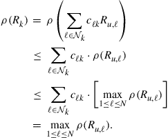
In other words,
![]()
It then follows from (9.198) that
![]()
so that (9.191) is satisfied as well.
Let us now examine the convergence rate. To begin with, we note that the matrix ![]() that appears in the weight-error recursion (9.189) is block diagonal:
that appears in the weight-error recursion (9.189) is block diagonal:
![]()
and each individual block entry, ![]() , is a stable matrix since
, is a stable matrix since ![]() satisfies (9.191). Moreover, each of these entries can be written as
satisfies (9.191). Moreover, each of these entries can be written as
![]()
which expresses ![]() as a convex combination of stable terms
as a convex combination of stable terms ![]() . Applying Jensen’s inequality again we get
. Applying Jensen’s inequality again we get
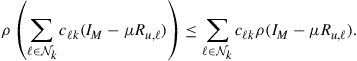
Now, we know from (9.189) that the rate of decay of ![]() to zero in the diffusion case is determined by the spectral radius of the coefficient matrix
to zero in the diffusion case is determined by the spectral radius of the coefficient matrix ![]() . Likewise, we know from (9.190) that the rate of decay of
. Likewise, we know from (9.190) that the rate of decay of ![]() to zero in the non-cooperative case is determined by the spectral radius of the coefficient matrix
to zero in the non-cooperative case is determined by the spectral radius of the coefficient matrix ![]() . Then, note that
. Then, note that
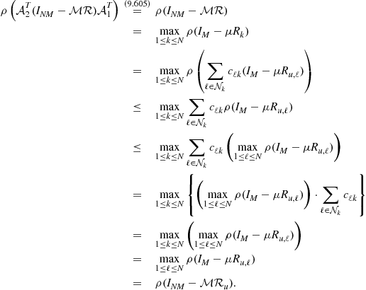
Therefore, the spectral radius of ![]() is at most as large as the largest individual spectral radius in the non-cooperative case.
is at most as large as the largest individual spectral radius in the non-cooperative case. ![]()
The argument can be modified to handle different step-sizes across the nodes if we assume uniform covariance data across the network, as stated below.
Theorem 9.5.4
Convergence Rate is Enhanced: Uniform Covariance Data
Consider the same setting of Theorem 9.5.3. Assume the covariance data are uniform across all nodes, say, ![]() is independent of
is independent of ![]() . Assume further that the nodes in both modes of operation employ steps-sizes
. Assume further that the nodes in both modes of operation employ steps-sizes ![]() that are chosen to satisfy the required stability conditions (9.191) and (9.194), which in this case are met by:
that are chosen to satisfy the required stability conditions (9.191) and (9.194), which in this case are met by:
![]() (9.199)
(9.199)
It then holds that the magnitude of the error vector, ![]() , in the diffusion case decays to zero more rapidly than in the non-cooperative case. In other words, diffusion enhances convergence rate.
, in the diffusion case decays to zero more rapidly than in the non-cooperative case. In other words, diffusion enhances convergence rate.
Proof.
Since ![]() for all
for all ![]() and
and ![]() is doubly stochastic, we get
is doubly stochastic, we get ![]() and
and ![]() . Then,
. Then,

![]()
The next statement considers the case of ATC and CTA strategies (9.137) and (9.145) without information exchange, which corresponds to the case ![]() . The result establishes that these strategies always enhance the convergence rate over the non-cooperative case, without the need to assume uniform step-sizes or uniform covariance data.
. The result establishes that these strategies always enhance the convergence rate over the non-cooperative case, without the need to assume uniform step-sizes or uniform covariance data.
Theorem 9.5.5
Convergence Rate is Enhanced when ![]()
Consider the problem of optimizing the global cost (9.92) with the individual cost functions given by (9.93). Pick left stochastic matrices ![]() and
and ![]() satisfying (9.166) and set
satisfying (9.166) and set ![]() . This situation covers the ATC and CTA strategies (9.137) and (9.145), which do not involve information exchange. Consider two modes of operation. In one mode, each node in the network runs the (distributed) steepest-descent diffusion algorithm (9.168)–(9.170). In the second mode, each node operates individually and runs the non-cooperative steepest-descent algorithm (9.171). In both cases, the positive step-sizes are chosen to satisfy the required stability conditions (9.193) and (9.194), which in this case are met by
. This situation covers the ATC and CTA strategies (9.137) and (9.145), which do not involve information exchange. Consider two modes of operation. In one mode, each node in the network runs the (distributed) steepest-descent diffusion algorithm (9.168)–(9.170). In the second mode, each node operates individually and runs the non-cooperative steepest-descent algorithm (9.171). In both cases, the positive step-sizes are chosen to satisfy the required stability conditions (9.193) and (9.194), which in this case are met by
![]() (9.200)
(9.200)
It then holds that the magnitude of the error vector, ![]() , in the diffusion case decays to zero more rapidly than in the non-cooperative case. In other words, diffusion cooperation enhances convergence rate.
, in the diffusion case decays to zero more rapidly than in the non-cooperative case. In other words, diffusion cooperation enhances convergence rate.
Proof.
When ![]() , we get
, we get ![]() and, therefore,
and, therefore, ![]() and
and ![]() . Then,
. Then,
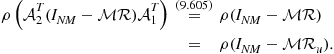
![]()
The results of the previous theorems highlight the following important facts about the role of the combination matrices ![]() in the convergence behavior of the diffusion strategy (9.163)–(9.165):
in the convergence behavior of the diffusion strategy (9.163)–(9.165):
a. The matrix ![]() influences the stability of the network through its influence on the bound in (9.191). This is because the matrices
influences the stability of the network through its influence on the bound in (9.191). This is because the matrices ![]() depend on the entries of
depend on the entries of ![]() . The matrices
. The matrices ![]() do not influence network stability in that they can be chosen arbitrarily and the network will remain stable under (9.191).
do not influence network stability in that they can be chosen arbitrarily and the network will remain stable under (9.191).
b. The matrices ![]() influence the rate of convergence of the network since they influence the spectral radius of the matrix
influence the rate of convergence of the network since they influence the spectral radius of the matrix ![]() , which controls the dynamics of the weight error vector in (9.189).
, which controls the dynamics of the weight error vector in (9.189).
3.09.6 Performance of adaptive diffusion strategies
We now move on to examine the behavior of the adaptive diffusion implementations (9.153) and (9.154), and the influence of both gradient noise and measurement noise on convergence and steady-state performance. Due to the random nature of the perturbations, it becomes necessary to evaluate the behavior of the algorithms on average, using mean-square convergence analysis. For this reason, we shall study the convergence of the weight estimates both in the mean and mean-square sense. To do so, we will again consider a general diffusion structure that includes the ATC and CTA strategies (9.153) and (9.154) as special cases. We shall further resort to the boldface notation to refer to the measurements and weight estimates in order to highlight the fact that they are now being treated as random variables. In this way, the update equations become stochastic updates. Thus, consider the following general adaptive diffusion strategy for ![]() :
:
![]() (9.201)
(9.201)
![]() (9.202)
(9.202)
![]() (9.203)
(9.203)
As before, the scalars ![]() are nonnegative real coefficients corresponding to the
are nonnegative real coefficients corresponding to the ![]() entries of
entries of ![]() combination matrices
combination matrices ![]() , respectively. These matrices are assumed to satisfy the same conditions (9.166) or (9.167). Again, different choices for
, respectively. These matrices are assumed to satisfy the same conditions (9.166) or (9.167). Again, different choices for ![]() correspond to different cooperation modes. For example, the choice
correspond to different cooperation modes. For example, the choice ![]() and
and ![]() corresponds to the adaptive ATC implementation (9.153), while the choice
corresponds to the adaptive ATC implementation (9.153), while the choice ![]() and
and ![]() corresponds to the adaptive CTA implementation (9.154). Likewise, the choice
corresponds to the adaptive CTA implementation (9.154). Likewise, the choice ![]() corresponds to the case in which the nodes only share weight estimates and the distributed diffusion recursions (9.201)–(9.203) become
corresponds to the case in which the nodes only share weight estimates and the distributed diffusion recursions (9.201)–(9.203) become
![]() (9.204)
(9.204)
![]() (9.205)
(9.205)
![]() (9.206)
(9.206)
Furthermore, the choice ![]() corresponds to the non-cooperative mode of operation, where each node runs the classical (stand-alone) least-mean-squares (LMS) filter independently of the other nodes [4–7]:
corresponds to the non-cooperative mode of operation, where each node runs the classical (stand-alone) least-mean-squares (LMS) filter independently of the other nodes [4–7]:
![]() (9.207)
(9.207)
3.09.6.1 Data model
When we studied the performance of the steepest-descent diffusion strategy (9.163)–(9.165) we exploited result (9.175), which indicated how the moments ![]() that appeared in the recursions related to the optimal solution
that appeared in the recursions related to the optimal solution ![]() . Likewise, in order to be able to analyze the performance of the adaptive diffusion strategy (9.201)–(9.203), we need to know how the data
. Likewise, in order to be able to analyze the performance of the adaptive diffusion strategy (9.201)–(9.203), we need to know how the data ![]() across the network relate to
across the network relate to ![]() . Motivated by the several examples presented earlier in Section 3.09.2, we shall assume that the data satisfy a linear model of the form:
. Motivated by the several examples presented earlier in Section 3.09.2, we shall assume that the data satisfy a linear model of the form:
![]() (9.208)
(9.208)
where ![]() is measurement noise with variance
is measurement noise with variance ![]() :
:
![]() (9.209)
(9.209)
and where the stochastic processes ![]() are assumed to be jointly wide-sense stationary with moments:
are assumed to be jointly wide-sense stationary with moments:
![]() (9.210)
(9.210)
![]() (9.211)
(9.211)
![]() (9.212)
(9.212)
All variables are assumed to be zero-mean. Furthermore, the noise process ![]() is assumed to be temporally white and spatially independent, as described earlier by (9.6), namely,
is assumed to be temporally white and spatially independent, as described earlier by (9.6), namely,
 (9.213)
The noise process ![]() is further assumed to be independent of the regression data
is further assumed to be independent of the regression data ![]() for all
for all ![]() and
and ![]() so that:
so that:
![]() (9.214)
(9.214)
We shall also assume that the regression data are temporally white and spatially independent so that:
![]() (9.215)
(9.215)
Although we are going to derive performance measures for the network under this independence assumption on the regression data, it turns out that the resulting expressions continue to match well with simulation results for sufficiently small step-sizes, even when the independence assumption does not hold (in a manner similar to the behavior of stand-alone adaptive filters) [4,5].
3.09.6.2 Performance measures
Our objective is to analyze whether, and how fast, the weight estimates ![]() from the adaptive diffusion implementation (9.201)–(9.203) converge towards
from the adaptive diffusion implementation (9.201)–(9.203) converge towards ![]() . To do so, we again introduce the
. To do so, we again introduce the ![]() weight error vectors:
weight error vectors:
![]() (9.216)
(9.216)
![]() (9.217)
(9.217)
![]() (9.218)
(9.218)
Each of these error vectors measures the residual relative to the desired ![]() in (9.208). We further introduce two scalar error measures:
in (9.208). We further introduce two scalar error measures:
![]() (9.219)
(9.219)
![]() (9.220)
(9.220)
The first error measures how well the term ![]() approximates the measured data,
approximates the measured data, ![]() ; in view of (9.208), this error can be interpreted as an estimator for the noise term
; in view of (9.208), this error can be interpreted as an estimator for the noise term ![]() . If node
. If node ![]() is able to estimate
is able to estimate ![]() well, then
well, then ![]() would get close to
would get close to ![]() . Therefore, under ideal conditions, we would expect the variance of
. Therefore, under ideal conditions, we would expect the variance of ![]() to tend towards the variance of
to tend towards the variance of ![]() . However, as remarked earlier in (9.31), there is generally an offset term for adaptive implementations that is captured by the variance of the a priori error,
. However, as remarked earlier in (9.31), there is generally an offset term for adaptive implementations that is captured by the variance of the a priori error, ![]() . This second error measures how well
. This second error measures how well ![]() approximates the uncorrupted term
approximates the uncorrupted term ![]() . Using the data model (9.208), we can relate
. Using the data model (9.208), we can relate ![]() as
as
![]() (9.221)
(9.221)
Since the noise component, ![]() , is assumed to be zero-mean and independent of all other random variables, we recover (9.31):
, is assumed to be zero-mean and independent of all other random variables, we recover (9.31):
![]() (9.222)
(9.222)
This relation confirms that the variance of the output error, ![]() is at least as large as
is at least as large as ![]() and away from it by an amount that is equal to the variance of the a priori error,
and away from it by an amount that is equal to the variance of the a priori error, ![]() . Accordingly, in order to quantify the performance of any particular node in the network, we define the mean-square-error (MSE) and excess-mean-square-error (EMSE) for node
. Accordingly, in order to quantify the performance of any particular node in the network, we define the mean-square-error (MSE) and excess-mean-square-error (EMSE) for node ![]() as the following steady-state measures:
as the following steady-state measures:
![]() (9.223)
(9.223)
![]() (9.224)
(9.224)
Then, it holds that
![]() (9.225)
(9.225)
Therefore, the EMSE term quantifies the size of the offset in the MSE performance of each node. We also define the mean-square-deviation (MSD) of each node as the steady-state measure:
![]() (9.226)
(9.226)
which measures how far ![]() is from
is from ![]() in the mean-square-error sense.
in the mean-square-error sense.
We indicated earlier in (9.36) and (9.37) how the MSD and EMSE of stand-alone LMS filters in the non-cooperative case depend on ![]() . In this section, we examine how cooperation among the nodes influences their performance. Since cooperation couples the operation of the nodes, with data originating from one node influencing the behavior of its neighbors and their neighbors, the study of the network performance requires more effort than in the non-cooperative case. Nevertheless, when all is said and done, we will arrive at expressions that approximate well the network performance and reveal some interesting conclusions.
. In this section, we examine how cooperation among the nodes influences their performance. Since cooperation couples the operation of the nodes, with data originating from one node influencing the behavior of its neighbors and their neighbors, the study of the network performance requires more effort than in the non-cooperative case. Nevertheless, when all is said and done, we will arrive at expressions that approximate well the network performance and reveal some interesting conclusions.
3.09.6.3 Error recursions
Using the data model (9.208) and subtracting ![]() from both sides of the relations in (9.201)–(9.203) we get
from both sides of the relations in (9.201)–(9.203) we get
![]() (9.227)
(9.227)
 (9.228)
![]() (9.229)
(9.229)
Comparing the second recursion with the corresponding recursion in the steepest-descent case (9.176)–(9.178), we see that two new effects arise: the effect of gradient noise, which replaces the covariance matrices ![]() by the instantaneous approximation
by the instantaneous approximation ![]() , and the effect of measurement noise,
, and the effect of measurement noise, ![]() .
.
We again describe the above relations more compactly by collecting the information from across the network in block vectors and matrices. We collect the error vectors from across all nodes into the following ![]() block vectors, whose individual entries are of size
block vectors, whose individual entries are of size ![]() each:
each:
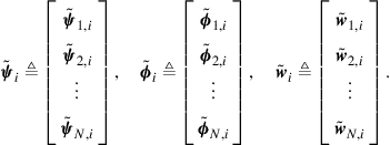 (9.230)
The block quantities ![]() represent the state of the errors across the network at time
represent the state of the errors across the network at time ![]() . Likewise, we introduce the following
. Likewise, we introduce the following ![]() block diagonal matrices, whose individual entries are of size
block diagonal matrices, whose individual entries are of size ![]() each:
each:
![]() (9.231)
(9.231)
 (9.232)
Each block diagonal entry of ![]() , say, the
, say, the ![]() th entry, contains a combination of rank-one regression terms collected from the neighborhood of node
th entry, contains a combination of rank-one regression terms collected from the neighborhood of node ![]() . In this way, the matrix
. In this way, the matrix ![]() is now stochastic and dependent on time, in contrast to the matrix
is now stochastic and dependent on time, in contrast to the matrix ![]() in the steepest-descent case in (9.181), which was a constant matrix. Nevertheless, it holds that
in the steepest-descent case in (9.181), which was a constant matrix. Nevertheless, it holds that
![]() (9.233)
(9.233)
so that, on average, ![]() agrees with
agrees with ![]() . We can simplify the notation by denoting the neighborhood combinations as follows:
. We can simplify the notation by denoting the neighborhood combinations as follows:
![]() (9.234)
(9.234)
![]() (9.235)
(9.235)
Again, compared with the matrix ![]() defined in (9.182), we find that
defined in (9.182), we find that ![]() is now both stochastic and time-dependent. Nevertheless, it again holds that
is now both stochastic and time-dependent. Nevertheless, it again holds that
![]() (9.236)
(9.236)
In the special case when ![]() , the matrix
, the matrix ![]() reduces to
reduces to
![]() (9.237)
(9.237)
with
![]() (9.238)
(9.238)
where ![]() was defined earlier in (9.184).
was defined earlier in (9.184).
We further introduce the following ![]() block column vector, whose entries are of size
block column vector, whose entries are of size ![]() each:
each:
![]() (9.239)
(9.239)
Obviously, given that the regression data and measurement noise are zero-mean and independent of each other, we have
![]() (9.240)
(9.240)
and the covariance matrix of ![]() is
is ![]() block diagonal with blocks of size
block diagonal with blocks of size ![]() :
:
![]() (9.241)
(9.241)
Returning to (9.227)–(9.229), we conclude that the following relations hold for the block quantities:
![]() (9.242)
(9.242)
![]() (9.243)
(9.243)
![]() (9.244)
(9.244)
where
![]() (9.245)
(9.245)
so that the network weight error vector, ![]() , ends up evolving according to the following stochastic recursion:
, ends up evolving according to the following stochastic recursion:
![]() (9.246)
(9.246)
For comparison purposes, if each node operates individually and uses the non-cooperative LMS recursion (9.207), then the weight error vector across all ![]() nodes would evolve according to the following stochastic recursion:
nodes would evolve according to the following stochastic recursion:
![]() (9.247)
(9.247)
where the matrices ![]() and
and ![]() do not appear, and
do not appear, and ![]() is replaced by
is replaced by ![]() from (9.237).
from (9.237).
3.09.6.4 Convergence in the mean
Taking expectations of both sides of (9.246) we find that:
![]() (9.248)
(9.248)
where we used the fact that ![]() and
and ![]() are independent of each other in view of our earlier assumptions on the regression data and noise in Section 3.09.6.1. Comparing with the error recursion (9.189) in the steepest-descent case, we find that both recursions are identical with
are independent of each other in view of our earlier assumptions on the regression data and noise in Section 3.09.6.1. Comparing with the error recursion (9.189) in the steepest-descent case, we find that both recursions are identical with ![]() replaced by
replaced by ![]() . Therefore, the convergence statements from the steepest-descent case can be extended to the adaptive case to provide conditions on the step-size to ensure stability in the mean, i.e., to ensure
. Therefore, the convergence statements from the steepest-descent case can be extended to the adaptive case to provide conditions on the step-size to ensure stability in the mean, i.e., to ensure
![]() (9.249)
(9.249)
When (9.249) is guaranteed, we say that the adaptive diffusion solution is asymptotically unbiased. The following statements restate the results of Theorems 9.5.1–9.5.5 in the context of mean error analysis.
Theorem 9.6.1
Convergence in the Mean
Consider the problem of optimizing the global cost (9.92) with the individual cost functions given by (9.93). Pick a right stochastic matrix ![]() and left stochastic matrices
and left stochastic matrices ![]() and
and ![]() satisfying (9.166) or (9.167). Assume each node in the network measures data that satisfy the conditions described in Section 3.09.6.1, and runs the adaptive diffusion algorithm (9.201)–(9.203). Then, all estimators
satisfying (9.166) or (9.167). Assume each node in the network measures data that satisfy the conditions described in Section 3.09.6.1, and runs the adaptive diffusion algorithm (9.201)–(9.203). Then, all estimators ![]() across the network converge in the mean to the optimal solution
across the network converge in the mean to the optimal solution ![]() if the positive step-size parameters
if the positive step-size parameters ![]() satisfy
satisfy
![]() (9.250)
(9.250)
where the neighborhood covariance matrix ![]() is defined by (9.182). In other words,
is defined by (9.182). In other words, ![]() for all nodes
for all nodes ![]() as
as ![]() .
.
Observe again that the mean stability condition (9.250) does not depend on the specific combination matrices ![]() and
and ![]() that are being used. Only the combination matrix
that are being used. Only the combination matrix ![]() influences the condition on the step-size through the neighborhood covariance matrices
influences the condition on the step-size through the neighborhood covariance matrices ![]() . Observe further that the statement of the lemma does not require the network to be connected. Moreover, when
. Observe further that the statement of the lemma does not require the network to be connected. Moreover, when ![]() , in which case the nodes only share weight estimators and do not share neighborhood data
, in which case the nodes only share weight estimators and do not share neighborhood data ![]() as in (9.204)–(9.206), condition (9.250) becomes
as in (9.204)–(9.206), condition (9.250) becomes
![]() (9.251)
(9.251)
Conditions (9.250) and (9.251) are reminiscent of a classical result for the stand-alone LMS algorithm, as in the non-cooperative case (9.207), where it is known that the estimator by each individual node in this case would converge in the mean to ![]() if, and only if, its step-size satisfies
if, and only if, its step-size satisfies
![]() (9.252)
(9.252)
The following statement provides a bi-directional result that ensures the mean convergence of the adaptive diffusion strategy for any choice of left-stochastic combination matrices ![]() and
and ![]() .
.
Theorem 9.6.2
Mean Convergence for Arbitrary Combination Matrices
Consider the problem of optimizing the global cost (9.92) with the individual cost functions given by (9.93). Pick a right stochastic matrix ![]() satisfying (9.166). Assume each node in the network measures data that satisfy the conditions described in Section 3.09.6.1. Then, the estimators
satisfying (9.166). Assume each node in the network measures data that satisfy the conditions described in Section 3.09.6.1. Then, the estimators ![]() generated by the adaptive diffusion strategy (9.201)–(9.203), converge in the mean to
generated by the adaptive diffusion strategy (9.201)–(9.203), converge in the mean to ![]() , for all choices of left stochastic matrices
, for all choices of left stochastic matrices ![]() and
and ![]() satisfying (9.166) if, and only if,
satisfying (9.166) if, and only if,
![]() (9.253)
(9.253)
As was the case with steepest-descent diffusion strategies, the adaptive diffusion strategy (9.201)–(9.203) also enhances the convergence rate of the mean of the error vector towards zero relative to the non-cooperative strategy (9.207). The next results restate Theorems 9.5.3–9.5.5; they assume ![]() is a doubly stochastic matrix.
is a doubly stochastic matrix.
Theorem 9.6.3
Mean Convergence Rate is Enhanced: Uniform Step-Sizes
Consider the problem of optimizing the global cost (9.92) with the individual cost functions given by (9.93). Pick a doubly stochastic matrix ![]() satisfying (9.196) and left stochastic matrices
satisfying (9.196) and left stochastic matrices ![]() and
and ![]() satisfying (9.166). Assume each node in the network measures data that satisfy the conditions described in Section 3.09.6.1. Consider two modes of operation. In one mode, each node in the network runs the adaptive diffusion algorithm (9.201)–(9.203). In the second mode, each node operates individually and runs the non-cooperative LMS algorithm (9.207). In both cases, the positive step-sizes used by all nodes are assumed to be the same, say,
satisfying (9.166). Assume each node in the network measures data that satisfy the conditions described in Section 3.09.6.1. Consider two modes of operation. In one mode, each node in the network runs the adaptive diffusion algorithm (9.201)–(9.203). In the second mode, each node operates individually and runs the non-cooperative LMS algorithm (9.207). In both cases, the positive step-sizes used by all nodes are assumed to be the same, say, ![]() for all
for all ![]() , and the value of
, and the value of ![]() is chosen to satisfy the required mean stability conditions (9.250) and (9.252), which are met by selecting
is chosen to satisfy the required mean stability conditions (9.250) and (9.252), which are met by selecting
![]() (9.254)
(9.254)
It then holds that the magnitude of the mean error vector, ![]() in the diffusion case decays to zero more rapidly than in the non-cooperative case. In other words, diffusion enhances convergence rate.
in the diffusion case decays to zero more rapidly than in the non-cooperative case. In other words, diffusion enhances convergence rate.
Theorem 9.6.4
Mean Convergence Rate is Enhanced: Uniform Covariance Data
Consider the same setting of Theorem 9.6.3. Assume the covariance data are uniform across all nodes, say, ![]() is independent of
is independent of ![]() . Assume further that the nodes in both modes of operation employ steps-sizes
. Assume further that the nodes in both modes of operation employ steps-sizes ![]() that are chosen to satisfy the required stability conditions (9.250) and (9.252), which in this case are met by:
that are chosen to satisfy the required stability conditions (9.250) and (9.252), which in this case are met by:
![]() (9.255)
(9.255)
It then holds that the magnitude of the mean error vector, ![]() in the diffusion case also decays to zero more rapidly than in the non-cooperative case. In other words, diffusion enhances convergence rate.
in the diffusion case also decays to zero more rapidly than in the non-cooperative case. In other words, diffusion enhances convergence rate.
The next statement considers the case of ATC and CTA strategies (9.204)–(9.206) without information exchange, which correspond to the choice ![]() . The result establishes that these strategies always enhance the convergence rate over the non-cooperative case, without the need to assume uniform step-sizes or uniform covariance data.
. The result establishes that these strategies always enhance the convergence rate over the non-cooperative case, without the need to assume uniform step-sizes or uniform covariance data.
Theorem 9.6.5
Mean Convergence Rate is Enhanced when ![]()
Consider the problem of optimizing the global cost (9.92) with the individual cost functions given by (9.93). Pick left stochastic matrices ![]() and
and ![]() satisfying (9.166) and set
satisfying (9.166) and set ![]() . This situation covers the ATC and CTA strategies (9.204)–(9.206) that do not involve information exchange. Assume each node in the network measures data that satisfy the conditions described in Section 3.09.6.1. Consider two modes of operation. In one mode, each node in the network runs the adaptive diffusion algorithm (9.163)–(9.165). In the second mode, each node operates individually and runs the non-cooperative LMS algorithm (9.207). In both cases, the positive step-sizes are chosen to satisfy the required stability conditions (9.251) and (9.252), which in this case are met by
. This situation covers the ATC and CTA strategies (9.204)–(9.206) that do not involve information exchange. Assume each node in the network measures data that satisfy the conditions described in Section 3.09.6.1. Consider two modes of operation. In one mode, each node in the network runs the adaptive diffusion algorithm (9.163)–(9.165). In the second mode, each node operates individually and runs the non-cooperative LMS algorithm (9.207). In both cases, the positive step-sizes are chosen to satisfy the required stability conditions (9.251) and (9.252), which in this case are met by
![]() (9.256)
(9.256)
It then holds that the magnitude of the mean error vector, ![]() in the diffusion case decays to zero more rapidly than in the non-cooperative case. In other words, diffusion cooperation enhances convergence rate.
in the diffusion case decays to zero more rapidly than in the non-cooperative case. In other words, diffusion cooperation enhances convergence rate.
The results of the previous theorems again highlight the following important facts about the role of the combination matrices ![]() in the convergence behavior of the adaptive diffusion strategy (9.201)–(9.203):
in the convergence behavior of the adaptive diffusion strategy (9.201)–(9.203):
a. The matrix ![]() influences the mean stability of the network through its influence on the bound in (9.250). This is because the matrices
influences the mean stability of the network through its influence on the bound in (9.250). This is because the matrices ![]() depend on the entries of
depend on the entries of ![]() . The matrices
. The matrices ![]() do not influence network mean stability in that they can be chosen arbitrarily and the network will remain stable under (9.250).
do not influence network mean stability in that they can be chosen arbitrarily and the network will remain stable under (9.250).
b. The matrices ![]() influence the rate of convergence of the mean weight-error vector over the network since they influence the spectral radius of the matrix
influence the rate of convergence of the mean weight-error vector over the network since they influence the spectral radius of the matrix ![]() , which controls the dynamics of the weight error vector in (9.248).
, which controls the dynamics of the weight error vector in (9.248).
3.09.6.5 Mean-square stability
It is not sufficient to ensure the stability of the weight-error vector in the mean sense. The error vectors, ![]() , may be converging on average to zero but they may have large fluctuations around the zero value. We therefore need to examine how small the error vectors get. To do so, we perform a mean-square-error analysis. The purpose of the analysis is to evaluate how the variances
, may be converging on average to zero but they may have large fluctuations around the zero value. We therefore need to examine how small the error vectors get. To do so, we perform a mean-square-error analysis. The purpose of the analysis is to evaluate how the variances ![]() evolve with time and what their steady-state values are, for each node
evolve with time and what their steady-state values are, for each node ![]() .
.
In this section, we are particularly interested in evaluating the evolution of two mean-square-errors, namely,
![]() (9.257)
(9.257)
The steady-state values of these quantities determine the MSD and EMSE performance levels at node ![]() and, therefore, convey critical information about the performance of the network. Under the independence assumption on the regression data from Section 3.09.6.1, it can be verified that the EMSE variance can be written as:
and, therefore, convey critical information about the performance of the network. Under the independence assumption on the regression data from Section 3.09.6.1, it can be verified that the EMSE variance can be written as:
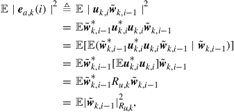 (9.258)
in terms of a weighted square measure with weighting matrix ![]() . Here we are using the notation
. Here we are using the notation ![]() to denote the weighted square quantity
to denote the weighted square quantity ![]() , for any column vector
, for any column vector ![]() and matrix
and matrix ![]() . Thus, we can evaluate mean-square-errors of the form (9.257) by evaluating the means of weighted square quantities of the following form:
. Thus, we can evaluate mean-square-errors of the form (9.257) by evaluating the means of weighted square quantities of the following form:
![]() (9.259)
(9.259)
for an arbitrary Hermitian nonnegative-definite weighting matrix ![]() that we are free to choose. By setting
that we are free to choose. By setting ![]() to different values (say,
to different values (say, ![]() or
or ![]() ), we can extract various types of information about the nodes and the network, as the discussion will reveal. The approach we follow is based on the energy conservation framework of [4,5,55].
), we can extract various types of information about the nodes and the network, as the discussion will reveal. The approach we follow is based on the energy conservation framework of [4,5,55].
So, let ![]() denote an arbitrary
denote an arbitrary ![]() block Hermitian nonnegative-definite matrix that we are free to choose, with
block Hermitian nonnegative-definite matrix that we are free to choose, with ![]() block entries
block entries ![]() . Let
. Let ![]() denote the
denote the ![]() vector that is obtained by stacking the columns of
vector that is obtained by stacking the columns of ![]() on top of each other, written as
on top of each other, written as
![]() (9.260)
(9.260)
In the sequel, it will become more convenient to work with the vector representation ![]() than with the matrix
than with the matrix ![]() itself.
itself.
We start from the weight-error vector recursion (9.246) and re-write it more compactly as:
![]() (9.261)
(9.261)
where the coefficient matrices ![]() and
and ![]() are short-hand representations for
are short-hand representations for
![]() (9.262)
(9.262)
and
![]() (9.263)
(9.263)
Note that ![]() is stochastic and time-variant, while
is stochastic and time-variant, while ![]() is constant. We denote the mean of
is constant. We denote the mean of ![]() by
by
![]() (9.264)
(9.264)
where ![]() is defined by (9.181). Now equating weighted square measures on both sides of (9.261) we get
is defined by (9.181). Now equating weighted square measures on both sides of (9.261) we get
![]() (9.265)
(9.265)
Expanding the right-hand side we find that
![]() (9.266)
(9.266)
Under expectation, the last two terms on the right-hand side evaluate to zero so that
![]() (9.267)
(9.267)
Let us evaluate each of the expectations on the right-hand side. The last expectation is given by
 (9.268)
where ![]() is defined by (9.241) and where we used the fact that
is defined by (9.241) and where we used the fact that ![]() for any two matrices
for any two matrices ![]() and
and ![]() of compatible dimensions. With regards to the first expectation on the right-hand side of (9.267), we have
of compatible dimensions. With regards to the first expectation on the right-hand side of (9.267), we have
 (9.269)
where we introduced the nonnegative-definite weighting matrix
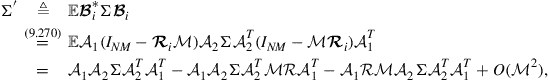 (9.270)
where ![]() is defined by (9.181) and the term
is defined by (9.181) and the term ![]() denotes the following factor, which depends on the square of the step-sizes,
denotes the following factor, which depends on the square of the step-sizes, ![]() :
:
![]() (9.271)
(9.271)
The evaluation of the above expectation depends on higher-order moments of the regression data. While we can continue with the analysis by taking this factor into account, as was done in [4,5,18,55], it is sufficient for the exposition in this chapter to focus on the case of sufficiently small step-sizes where terms involving higher powers of the step-sizes can be ignored. Therefore, we continue our discussion by letting
![]() (9.272)
(9.272)
The weighting matrix ![]() is fully defined in terms of the step-size matrix,
is fully defined in terms of the step-size matrix, ![]() , the network topology through the matrices
, the network topology through the matrices ![]() , and the regression statistical profile through
, and the regression statistical profile through ![]() . Expression (9.272) tells us how to construct
. Expression (9.272) tells us how to construct ![]() from
from ![]() . The expression can be transformed into a more compact and revealing form if we instead relate the vector forms
. The expression can be transformed into a more compact and revealing form if we instead relate the vector forms ![]() and
and ![]() . Using the following equalities for arbitrary matrices
. Using the following equalities for arbitrary matrices ![]() of compatible dimensions [5]:
of compatible dimensions [5]:
![]() (9.273)
(9.273)
![]() (9.274)
(9.274)
and applying the vec operation to both sides of (9.272) we get
![]()
That is,
![]() (9.275)
(9.275)
where we are introducing the coefficient matrix of size ![]() :
:
![]() (9.276)
(9.276)
A reasonable approximate expression for ![]() for sufficiently small step-sizes is
for sufficiently small step-sizes is
![]() (9.277)
(9.277)
Indeed, if we replace ![]() from (9.264) into (9.277) and expand terms, we obtain the same factors that appear in (9.276) plus an additional term that depends on the square of the step-sizes,
from (9.264) into (9.277) and expand terms, we obtain the same factors that appear in (9.276) plus an additional term that depends on the square of the step-sizes, ![]() , whose effect can be ignored for sufficiently small step-sizes.
, whose effect can be ignored for sufficiently small step-sizes.
In this way, and using in addition property (9.274), we find that relation (9.267) becomes:
![]() (9.278)
(9.278)
The last term is dependent on the network topology through the matrix ![]() , which is defined in terms of
, which is defined in terms of ![]() , and the noise and regression data statistical profile through
, and the noise and regression data statistical profile through ![]() . It is convenient to introduce the alternative notation
. It is convenient to introduce the alternative notation ![]() to refer to the weighted square quantity
to refer to the weighted square quantity ![]() , where
, where ![]() . We shall use these two notations interchangeably. The convenience of the vector notation is that it allows us to exploit the simpler linear relation (9.275) between
. We shall use these two notations interchangeably. The convenience of the vector notation is that it allows us to exploit the simpler linear relation (9.275) between ![]() and
and ![]() to rewrite (9.278) as shown in (9.279) below, with the same weight vector
to rewrite (9.278) as shown in (9.279) below, with the same weight vector ![]() appearing on both sides.
appearing on both sides.
Theorem 9.6.6
Variance Relation
Consider the data model of Section 3.09.6.1 and the independence statistical conditions imposed on the noise and regression data, including (9.208)–(9.215). Assume further sufficiently small step-sizes are used so that terms that depend on higher-powers of the step-sizes can be ignored. Pick left stochastic matrices ![]() and
and ![]() and a right stochastic matrix
and a right stochastic matrix ![]() satisfying (9.166). Under these conditions, the weight-error vector
satisfying (9.166). Under these conditions, the weight-error vector ![]() associated with a network running the adaptive diffusion strategy (9.201)–(9.203) satisfies the following variance relation:
associated with a network running the adaptive diffusion strategy (9.201)–(9.203) satisfies the following variance relation:
![]() (9.279)
(9.279)
for any Hermitian nonnegative-definite matrix ![]() with
with ![]() , and where
, and where ![]() are defined by (9.241), (9.263), and (9.277), and
are defined by (9.241), (9.263), and (9.277), and
![]() (9.280)
(9.280)
![]()
Note that relation (9.279) is not an actual recursion; this is because the weighting matrices ![]() on both sides of the equality are different. The relation can be transformed into a true recursion by expanding it into a convenient state-space model; this argument was pursued in [4,5,18,55] and is not necessary for the exposition here, except to say that stability of the matrix
on both sides of the equality are different. The relation can be transformed into a true recursion by expanding it into a convenient state-space model; this argument was pursued in [4,5,18,55] and is not necessary for the exposition here, except to say that stability of the matrix ![]() ensures the mean-square stability of the filter—this fact is also established further ahead through relation (9.327). By mean-square stability we mean that each term
ensures the mean-square stability of the filter—this fact is also established further ahead through relation (9.327). By mean-square stability we mean that each term ![]() remains bounded over time and converges to a steady-state
remains bounded over time and converges to a steady-state ![]() value. Moreover, the spectral radius of
value. Moreover, the spectral radius of ![]() controls the rate of convergence of
controls the rate of convergence of ![]() towards its steady-state value.
towards its steady-state value.
Theorem 9.6.7
Mean-Square Stability
Consider the same setting of Theorem 9.6.6. The adaptive diffusion strategy (9.201)–(9.203) is mean-square stable if, and only if, the matrix ![]() defined by (9.276), or its approximation (9.277), is stable (i.e., all its eigenvalues lie strictly inside the unit disc). This condition is satisfied by sufficiently small positive step-sizes
defined by (9.276), or its approximation (9.277), is stable (i.e., all its eigenvalues lie strictly inside the unit disc). This condition is satisfied by sufficiently small positive step-sizes ![]() that are also smaller than the following bound:
that are also smaller than the following bound:
![]() (9.281)
(9.281)
where the neighborhood covariance matrix ![]() is defined by (9.182). Moreover, the convergence rate of the algorithm is determined by the value
is defined by (9.182). Moreover, the convergence rate of the algorithm is determined by the value ![]() (the square of the spectral radius of
(the square of the spectral radius of ![]() ).
).
Proof.
Recall that, for two arbitrary matrices ![]() and
and ![]() of compatible dimensions, the eigenvalues of the Kronecker product
of compatible dimensions, the eigenvalues of the Kronecker product ![]() is formed of all product combinations
is formed of all product combinations ![]() of the eigenvalues of
of the eigenvalues of ![]() and
and ![]() [19]. Therefore, for sufficiently small step-sizes, we can use expression (9.277) to note that
[19]. Therefore, for sufficiently small step-sizes, we can use expression (9.277) to note that ![]() . It follows that
. It follows that ![]() is stable if, and only if,
is stable if, and only if, ![]() is stable. We already noted earlier in Theorem 9.6.1 that condition (9.281) ensures the stability of
is stable. We already noted earlier in Theorem 9.6.1 that condition (9.281) ensures the stability of ![]() . Therefore, step-sizes that ensure stability in the mean and are sufficiently small will also ensure mean-square stability.
. Therefore, step-sizes that ensure stability in the mean and are sufficiently small will also ensure mean-square stability. ![]()
Remark
More generally, had we not ignored the second-order term (9.271), the expression for ![]() would have been the following. Starting from the definition
would have been the following. Starting from the definition ![]() , we would get
, we would get
![]()
so that
![]() (9.282)
(9.282)
![]()
Mean-square stability of the filter would then require the step-sizes ![]() to be chosen such that they ensure the stability of this matrix
to be chosen such that they ensure the stability of this matrix ![]() (in addition to condition (9.281) to ensure mean stability).
(in addition to condition (9.281) to ensure mean stability). ![]()
3.09.6.6 Network mean-square performance
We can now use the variance relation (9.279) to evaluate the network performance, as well as the performance of the individual nodes, in steady-state. Since the dynamics is mean-square stable for sufficiently small step-sizes, we take the limit of (9.279) as ![]() and write:
and write:
![]() (9.283)
(9.283)
Grouping terms leads to the following result.
Corollary 9.6.1
Steady-State Variance Relation
Consider the same setting of Theorem 9.6.6. The weight-error vector, ![]() of the adaptive diffusion strategy (9.201)–(9.203) satisfies the following relation in steady-state:
of the adaptive diffusion strategy (9.201)–(9.203) satisfies the following relation in steady-state:
![]() (9.284)
(9.284)
for any Hermitian nonnegative-definite matrix ![]() with
with ![]() , and where
, and where ![]() are defined by (9.277) and (9.280).
are defined by (9.277) and (9.280).
![]()
Expression (9.284) is a very useful relation; it allows us to evaluate the network MSD and EMSE through proper selection of the weighting vector ![]() (or, equivalently, the weighting matrix
(or, equivalently, the weighting matrix ![]() ). For example, the network MSD is defined as the average value:
). For example, the network MSD is defined as the average value:
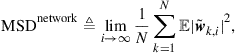 (9.285)
which amounts to averaging the MSDs of the individual nodes. Therefore,
![]() (9.286)
(9.286)
This means that in order to recover the network MSD from relation (9.284), we should select the weighting vector ![]() such that
such that
![]()
Solving for ![]() and substituting back into (9.284) we arrive at the following expression for the network MSD:
and substituting back into (9.284) we arrive at the following expression for the network MSD:
![]() (9.287)
(9.287)
Likewise, the network EMSE is defined as the average value
 (9.288)
which amounts to averaging the EMSEs of the individual nodes. Therefore,
![]() (9.289)
(9.289)
where ![]() is the matrix defined earlier by (9.184), and which we repeat below for ease of reference:
is the matrix defined earlier by (9.184), and which we repeat below for ease of reference:
![]() (9.290)
(9.290)
This means that in order to recover the network EMSE from relation (9.284), we should select the weighting vector ![]() such that
such that
![]() (9.291)
(9.291)
Solving for ![]() and substituting into (9.284) we arrive at the following expression for the network EMSE:
and substituting into (9.284) we arrive at the following expression for the network EMSE:
![]() (9.292)
(9.292)
3.09.6.7 Mean-square performance of individual nodes
We can also assess the mean-square performance of the individual nodes in the network from (9.284). For instance, the MSD of any particular node ![]() is defined by
is defined by
![]() (9.293)
(9.293)
Introduce the ![]() block diagonal matrix with blocks of size
block diagonal matrix with blocks of size ![]() , where all blocks on the diagonal are zero except for an identity matrix on the diagonal block of index
, where all blocks on the diagonal are zero except for an identity matrix on the diagonal block of index ![]() , i.e.,
, i.e.,
![]() (9.294)
(9.294)
Then, we can express the node MSD as follows:
![]() (9.295)
(9.295)
The same argument that was used to obtain the network MSD then leads to
![]() (9.296)
(9.296)
Likewise, the EMSE of node ![]() is defined by
is defined by
 (9.297)
Introduce the ![]() block diagonal matrix with blocks of size
block diagonal matrix with blocks of size ![]() , where all blocks on the diagonal are zero except for the diagonal block of index
, where all blocks on the diagonal are zero except for the diagonal block of index ![]() whose value is
whose value is ![]() , i.e.,
, i.e.,
![]() (9.298)
(9.298)
Then, we can express the node EMSE as follows:
![]() (9.299)
(9.299)
The same argument that was used to obtain the network EMSE then leads to
![]() (9.300)
(9.300)
We summarize the results in the following statement.
Theorem 9.6.8
Network Mean-Square Performance
Consider the same setting of Theorem 9.6.6. Introduce the ![]() row vector
row vector ![]() defined by
defined by
![]() (9.301)
(9.301)
where ![]() are defined by (9.277) and (9.280). Then the network MSD and EMSE and the individual node performance measures are given by
are defined by (9.277) and (9.280). Then the network MSD and EMSE and the individual node performance measures are given by
![]() (9.302)
(9.302)
![]() (9.303)
(9.303)
![]() (9.304)
(9.304)
![]() (9.305)
(9.305)
where ![]() are defined by (9.294) and (9.298).
are defined by (9.294) and (9.298).
![]()
We can recover from the above expressions the performance of the nodes in the non-cooperative implementation (9.207), where each node performs its adaptation individually, by setting ![]() .
.
We can express the network MSD, and its EMSE if desired, in an alternative useful form involving a series representation.
Corollary 9.6.2
Series Representation for Network MSD
Consider the same setting of Theorem 9.6.6. The network MSD can be expressed in the following alternative series form:
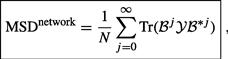 (9.306)
where
![]() (9.307)
(9.307)
![]() (9.308)
(9.308)
![]() (9.309)
(9.309)
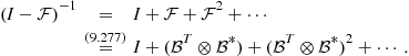
3.09.6.8 Uniform data profile
We can simplify expressions (9.307)–(9.309) for ![]() in the case when the regression covariance matrices are uniform across the network and all nodes employ the same step-size, i.e., when
in the case when the regression covariance matrices are uniform across the network and all nodes employ the same step-size, i.e., when
![]() (9.310)
(9.310)
![]() (9.311)
(9.311)
and when the combination matrix ![]() is doubly stochastic, so that
is doubly stochastic, so that
![]() (9.312)
(9.312)
Thus, under conditions (9.310)–(9.312), expressions (9.180), (9.181), and (9.263) for ![]() simplify to
simplify to
![]() (9.313)
(9.313)
![]() (9.314)
(9.314)
![]() (9.315)
(9.315)
Substituting these values into expression (9.309) for ![]() we get
we get
 (9.316)
where we used the useful Kronecker product identities:
![]() (9.317)
(9.317)
![]() (9.318)
(9.318)
for any matrices ![]() of compatible dimensions. Likewise, introduce the
of compatible dimensions. Likewise, introduce the ![]() diagonal matrix with noise variances:
diagonal matrix with noise variances:
![]() (9.319)
(9.319)
Then, expression (9.241) for ![]() becomes
becomes
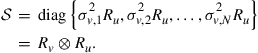 (9.320)
It then follows that we can simplify expression (9.307) for ![]() as:
as:
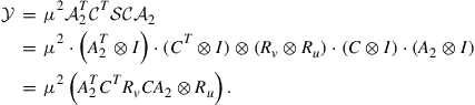 (9.321)
Corollary 9.6.3
Network MSD for Uniform Data Profile
Consider the same setting of Theorem 9.6.6 with the additional requirement that conditions (9.310)–(9.312) for a uniform data profile hold. The network MSD is still given by the same series representation (9.306) where now
![]() (9.322)
(9.322)
![]() (9.323)
(9.323)
Using these expressions, we can decouple the network MSD expression (9.306) into two separate factors: one is dependent on the step-size and data covariance ![]() , and the other is dependent on the combination matrices and noise profile
, and the other is dependent on the combination matrices and noise profile ![]() :
:
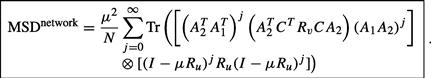 (9.324)
![]()
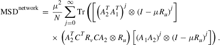
3.09.6.9 Transient mean-square performance
Before comparing the mean-square performance of various cooperation strategies, we pause to comment that the variance relation (9.279) can also be used to characterize the transient behavior of the network, and not just its steady-state performance. To see this, iterating (9.279) starting from ![]() , we find that
, we find that
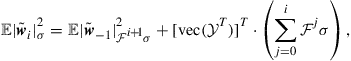 (9.325)
![]() (9.326)
(9.326)
in terms of the initial condition, ![]() . If this initial condition happens to be
. If this initial condition happens to be ![]() , then
, then ![]() . Comparing expression (9.325) at time instants
. Comparing expression (9.325) at time instants ![]() and
and ![]() we can relate
we can relate ![]() and
and ![]() as follows:
as follows:
![]() (9.327)
(9.327)
This recursion relates the same weighted square measures of the error vectors ![]() . It therefore describes how these weighted square measures evolve over time. It is clear from this relation that, for mean-square stability, the matrix
. It therefore describes how these weighted square measures evolve over time. It is clear from this relation that, for mean-square stability, the matrix ![]() needs to be stable so that the terms involving
needs to be stable so that the terms involving ![]() do not grow unbounded.
do not grow unbounded.
The learning curve of the network is the curve that describes the evolution of the network EMSE over time. At any time ![]() , the network EMSE is denoted by
, the network EMSE is denoted by ![]() and measured as:
and measured as:
 (9.328)
The above expression indicates that ![]() is obtained by averaging the EMSE of the individual nodes at time
is obtained by averaging the EMSE of the individual nodes at time ![]() . Therefore,
. Therefore,
![]() (9.329)
(9.329)
where ![]() is the matrix defined by (9.290). This means that in order to evaluate the evolution of the network EMSE from relation (9.327), we simply select the weighting vector
is the matrix defined by (9.290). This means that in order to evaluate the evolution of the network EMSE from relation (9.327), we simply select the weighting vector ![]() such that
such that
![]() (9.330)
(9.330)
Substituting into (9.327) we arrive at the learning curve for the network.
Corollary 9.6.4
Network Learning Curve
Consider the same setting of Theorem 9.6.6. Let ![]() denote the network EMSE at time
denote the network EMSE at time ![]() , as defined by (9.328). Then, the learning curve of the network corresponds to the evolution of
, as defined by (9.328). Then, the learning curve of the network corresponds to the evolution of ![]() with time and is described by the following recursion over
with time and is described by the following recursion over ![]() :
:
![]() (9.331)
(9.331)