
Bayesian Computational Methods in Signal Processing
Simon Godsill, Signal Processing and Communications Laboratory, Department of Engineering, University of Cambridge, UK
Abstract
In this article we give an introductory survey of Bayesian statistical methods applied to signal processing models, with an emphasis on computational techniques such as expectation-maximization and Monte Carlo inference (batch and sequential). The area is now highly evolved and sophisticated, and hence it is not practical to cover all topics of current research; however we hope that this article will teach some of the basics and inspire the reader to go on and study the rich families of statistical methodology that are still evolving under the Bayesian heading.
3.04.1 Introduction
Over recent decades Bayesian computational techniques have risen from relative obscurity to becoming one of the principal means of solving complex statistical signal processing problems. Methodology is now mature and sophisticated. This article aims to provide a brief and basic introduction for those starting on the topic, with the aim of inspiring further research work in this vibrant area.
The paper is structured as follows. Section 3.04.2 covers Bayesian parameter estimation, with a worked case study in Bayesian linear Gaussian models. This section also introduces model uncertainty from a Bayesian perspective. Section 3.04.3 introduces some of the computational tools available for batch inference, including the expectation-maximization (EM) algorithm and the Markov chain Monte Carlo (MCMC) algorithm. Section 3.04.4 moves on to sequential inference problems, covering linear state-space models, Kalman filters, nonlinear state-space models, and particle filtering.
3.04.2 Parameter estimation
In parameter estimation we suppose that a random process ![]() depends in some well-defined stochastic manner upon an unobserved parameter vector
depends in some well-defined stochastic manner upon an unobserved parameter vector ![]() . If we observe N data points from the random process, we can form a vector
. If we observe N data points from the random process, we can form a vector ![]() . The parameter estimation problem is to deduce the value of
. The parameter estimation problem is to deduce the value of ![]() from the observations
from the observations ![]() . In general it will not be possible to deduce the parameters exactly from a finite number of data points since the process is random, but various schemes will be described which achieve different levels of performance depending upon the amount of data available and the amount of prior information available regarding
. In general it will not be possible to deduce the parameters exactly from a finite number of data points since the process is random, but various schemes will be described which achieve different levels of performance depending upon the amount of data available and the amount of prior information available regarding ![]() .
.
We now define a general parametric model, the linear Gaussian model, which will be referred to frequently in this and subsequent sections. This model will be used as a motivating example in much of the work in this section, with details of the calculations required to perform the various aspects of inference in classical and Bayesian settings. This model is a fundamental building block for many more complex and sophisticated non-linear or non-Gaussian models in signal processing, and so these fundamentals will be referred to numerous times later in the text. However, although we use these models as a motivating example throughout the early sections, it should be borne in mind that there are indeed many classes of model in practical application that have none, or very little, linear Gaussian structure, and for these results specialized techniques are required for inference; none of the analytic results here will apply in these cases, but the fundamental structure of the Bayesian inference methodology does indeed carry through unchanged, and inference can still be successfully performed, albeit with more effort and typically greater computational burden. The Monte Carlo methods described later, and in particular the particle filtering and Markov chain Monte Carlo (MCMC) approaches, are well suited to inference in the hardest models with no apparent linear or Gaussian structure.
Another class of model that is amenable to certain simple analytic computations beyond the linear Gaussian class is the discrete Markov chain model and its counterpart the hidden Markov model (HMM). This model, not covered in this tutorial, can readily be combined with linear Gaussian structures to yield sophisticated switching models that can be elegantly inferred within the fully Bayesian framework.
3.04.2.1 The linear Gaussian model
In the general model it is assumed that the data ![]() are generated as a function of the parameters
are generated as a function of the parameters ![]() with a random modeling error term
with a random modeling error term ![]() :
:
![]()
where ![]() is a deterministic and possibly non-linear function of the parameter
is a deterministic and possibly non-linear function of the parameter ![]() and the random error, or “disturbance”
and the random error, or “disturbance” ![]() . Now we will consider the important special case where the function is linear and the error is additive, so we may write
. Now we will consider the important special case where the function is linear and the error is additive, so we may write
![]()
where ![]() is a P-dimensional column vector, and the expression may be written for the whole vector
is a P-dimensional column vector, and the expression may be written for the whole vector ![]() as
as
![]() (4.1)
(4.1)
where

The columns ![]() of
of ![]() form a fixed basis vector representation of the data, for example sinusoidsof different frequencies in a signal which is known to be made up of pure frequency components in noise. A variant of this model will be seen later in the section, the autoregressive (AR) model, in which previous data points are used to predict the current data point
form a fixed basis vector representation of the data, for example sinusoidsof different frequencies in a signal which is known to be made up of pure frequency components in noise. A variant of this model will be seen later in the section, the autoregressive (AR) model, in which previous data points are used to predict the current data point ![]() . The error sequence
. The error sequence ![]() will usually (but not necessarily) be assumed drawn from an independent, identically distributed (i.i.d.) noise distribution, that is,
will usually (but not necessarily) be assumed drawn from an independent, identically distributed (i.i.d.) noise distribution, that is,
![]()
where ![]() denotes some noise distribution which is identical for all n. Note that some powerful models can be constructed using heterogeneous noise sources, in which the distribution
denotes some noise distribution which is identical for all n. Note that some powerful models can be constructed using heterogeneous noise sources, in which the distribution ![]() can vary with n. This might be for the purpose of modeling a time-varying noise term, or for modeling a heavy-tailed noise distribution through the introduction of additional latent variables at each time point.1
can vary with n. This might be for the purpose of modeling a time-varying noise term, or for modeling a heavy-tailed noise distribution through the introduction of additional latent variables at each time point.1![]() can be viewed as a modeling error, innovationor observation noise, depending upon the type of model. When
can be viewed as a modeling error, innovationor observation noise, depending upon the type of model. When ![]() is the normal distribution and
is the normal distribution and ![]() is a linear function, we have the linear Gaussian model.
is a linear function, we have the linear Gaussian model.
There are many examples of the use of such a linear Gaussian modeling framework. Two very simple and standard cases are the sinusoidal model and the autoregressive (AR) model.
Example
(Sinusoidal model) If we write a single sinusoid as the sum of sine and cosine components we have:
![]()
Thus we can form a second order (![]() ) linear model from this if we take:
) linear model from this if we take:

where
![]()
and
![]()
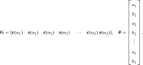
And similarly, if the model is composed of J sinusoids at different frequencies ![]() we have
we have
![]()
and the linear model expression is
Example
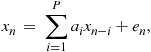
(Autoregressive (AR) model) The AR model is a standard time series model based on an all-pole filtered version of the noise residual:
 (4.2)
(4.2)
The coefficients ![]() are the filter coefficients of the all-pole filter, henceforth referred to as the AR parameters, and P, the number of coefficients, is the order of the AR process. The AR model formulation is closely related to the linear prediction framework used in many fields of signal processing (see e.g., [1,2]). The AR modeling equation of (4.2) is now rewritten for the block of N data samples as
are the filter coefficients of the all-pole filter, henceforth referred to as the AR parameters, and P, the number of coefficients, is the order of the AR process. The AR model formulation is closely related to the linear prediction framework used in many fields of signal processing (see e.g., [1,2]). The AR modeling equation of (4.2) is now rewritten for the block of N data samples as
![]() (4.3)
(4.3)
where ![]() is the vector of
is the vector of ![]() error values and the (
error values and the (![]() ) matrix
) matrix ![]() is given by
is given by
 (4.4)
(4.4)
3.04.2.2 Maximum likelihood (ML) estimation
Prior to consideration of Bayesian approaches, we first present the maximum likelihood (ML) estimator, which treats the parameters as unknown constants about which we incorporate no prior information. The observed data ![]() is, however, considered random and we can often then obtain the PDF for
is, however, considered random and we can often then obtain the PDF for ![]() when the value of
when the value of ![]() is known. This PDF is termed the likelihood
is known. This PDF is termed the likelihood ![]() , which is defined as
, which is defined as
![]() (4.5)
(4.5)
The likelihood is of course implicitly conditioned upon all of our modeling assumptions ![]() , which could more properly be expressed as
, which could more properly be expressed as ![]() .
.
The ML estimate for ![]() is then that value of
is then that value of ![]() which maximizes the likelihood for given observations
which maximizes the likelihood for given observations ![]() :
:
![]() (4.6)
(4.6)
Maximum likelihood (ML) estimator.
The rationale behind this is that the ML solution corresponds to the parameter vector which would have generated the observed data ![]() with highest probability. The maximization task required for ML estimation can be achieved using standard differential calculus for well-behaved and differentiable likelihood functions, and it is often convenient analytically to maximize the log-likelihood function
with highest probability. The maximization task required for ML estimation can be achieved using standard differential calculus for well-behaved and differentiable likelihood functions, and it is often convenient analytically to maximize the log-likelihood function ![]() rather than
rather than ![]() itself. Since
itself. Since ![]() is a monotonically increasing function the two solutions are identical.
is a monotonically increasing function the two solutions are identical.
In data analysis and signal processing applications the likelihood function is arrived at through knowledge of the stochastic model for the data. For example, in the case of the linear Gaussian model (4.1) the likelihood can be obtained easily if we know the form of ![]() , the joint PDF for the components of the error vector. The likelihood
, the joint PDF for the components of the error vector. The likelihood ![]() is then found from a transformation of variables
is then found from a transformation of variables ![]() where
where ![]() . The Jacobian for this transformation is unity, so the likelihood is:
. The Jacobian for this transformation is unity, so the likelihood is:
![]() (4.7)
(4.7)
The ML solution may of course be posed for any error distribution, including highly non-Gaussian and non-independent cases. Here we give the most straightforward case, for the linear model where the elements of the error vector ![]() are assumed to be i.i.d. and Gaussian and zero mean. If the variance of the Gaussian is
are assumed to be i.i.d. and Gaussian and zero mean. If the variance of the Gaussian is ![]() we then have:
we then have:

 (4.8)
(4.8)
which leads to the following log-likelihood expression:

Maximization of this function w.r.t. ![]() is equivalent to minimizing the sum-squared of the error sequence
is equivalent to minimizing the sum-squared of the error sequence ![]() . This is exactly the criterion which is applied in the familiar least squares (LS) estimation method. The ML estimator is obtained by taking derivatives w.r.t.
. This is exactly the criterion which is applied in the familiar least squares (LS) estimation method. The ML estimator is obtained by taking derivatives w.r.t. ![]() and equating to zero:
and equating to zero:
![]() (4.9)
(4.9)
Maximum likelihood for the linear Gaussian model, which is, as expected, the familiar linear least squares estimate for model parameters calculated from finite length data observations. Thus we see that the ML estimator under the i.i.d. Gaussian error assumption is exactly equivalent to the well known least squares (LS) parameter estimator.
3.04.2.3 Bayesian inference
The ML methods treat parameters as unknown constants. If we are prepared to treat parameters as random variables it is possible to assign prior PDFs to the parameters. These PDFs should ideally express some prior knowledge about the relative probability of different parameter values before the data are observed. Of course if nothing is known a priori about the parameters then the prior distributions should in some sense express no initial preference for one set of parameters over any other. Note that in many cases a prior density is chosen to express some highly qualitative prior knowledge about the parameters. In such cases the prior chosen will be more a reflection of a degree of belief concerning parameter values than any true modeling of an underlying random process which might have generated those parameters. This willingness to assign priors which reflect subjective information is a powerful feature and also one of the most fundamental differences between the Bayesian and “classical” inferential procedures. For various expositions of the Bayesian methodology and philosophy see, for example [3–6]. The precise form of probability distributions assigned a priori to the parameters requires careful consideration since misleading results can be obtained from erroneous priors, but in principle at least we can apply the Bayesian approach to any problem where statistical uncertainty is present.
Bayes’ theorem is now stated as applied to estimation of random parameters ![]() from a random vector
from a random vector ![]() of observations, known as the posterior or a posteriori probability for the parameter:
of observations, known as the posterior or a posteriori probability for the parameter:
![]() (4.10)
(4.10)
Posterior probability. Note that all of the distributions in this expression are implicitly conditioned upon all prior modeling assumptions, as was the likelihood function earlier. The distribution ![]() is the likelihood as used for ML estimation, while
is the likelihood as used for ML estimation, while ![]() is the prior or a priori distribution for the parameters. This term is one of the critical differences between Bayesian and “classical” techniques. It expresses in an objective fashion the probability of various model parameters values before the data
is the prior or a priori distribution for the parameters. This term is one of the critical differences between Bayesian and “classical” techniques. It expresses in an objective fashion the probability of various model parameters values before the data ![]() has been observed. As we have already observed, the prior density may be an expression of highly subjective information about parameter values. This transformation from the subjective domain to an objective form for the prior can clearly be of great significance and should be considered carefully when setting up an inference problem.
has been observed. As we have already observed, the prior density may be an expression of highly subjective information about parameter values. This transformation from the subjective domain to an objective form for the prior can clearly be of great significance and should be considered carefully when setting up an inference problem.
The term ![]() , the posterior or a posteriori distribution, expresses the probability of
, the posterior or a posteriori distribution, expresses the probability of ![]() given the observed data
given the observed data ![]() . This is now a true measure of how “probable” a particular value of
. This is now a true measure of how “probable” a particular value of ![]() is, given the observations
is, given the observations ![]() .
. ![]() is in a more intuitive form for parameter estimation than the likelihood, which expresses how probable the observations are given the parameters. The generation of the posterior distribution from the prior distribution when data
is in a more intuitive form for parameter estimation than the likelihood, which expresses how probable the observations are given the parameters. The generation of the posterior distribution from the prior distribution when data ![]() is observed can be thought of as a refinement to any previous (“prior”) knowledge about the parameters. Before
is observed can be thought of as a refinement to any previous (“prior”) knowledge about the parameters. Before ![]() is observed
is observed ![]() expresses any information previously obtained concerning
expresses any information previously obtained concerning ![]() . Any new information concerning the parameters contained in
. Any new information concerning the parameters contained in ![]() is then incorporated to give the posterior distribution. Clearly if we start off with little or no information about
is then incorporated to give the posterior distribution. Clearly if we start off with little or no information about ![]() then the posterior distribution is likely to obtain information obtained almost solely from
then the posterior distribution is likely to obtain information obtained almost solely from ![]() . Conversely, if
. Conversely, if ![]() expresses a significant amount of information about
expresses a significant amount of information about ![]() then
then ![]() will contribute less new information to the posterior distribution.
will contribute less new information to the posterior distribution.
The denominator ![]() , referred to as the marginal likelihood, or the “evidence” in machine learning circles, is a fundamentally useful quantity in model selection problems (see later), and is constant for any given observation
, referred to as the marginal likelihood, or the “evidence” in machine learning circles, is a fundamentally useful quantity in model selection problems (see later), and is constant for any given observation ![]() ; thus it may be ignored if we are only interested in the relative posterior probabilities of different parameters. As a result of this, Bayes’ theorem is often stated in the form:
; thus it may be ignored if we are only interested in the relative posterior probabilities of different parameters. As a result of this, Bayes’ theorem is often stated in the form:
![]() (4.11)
(4.11)
Posterior probability (proportionality).
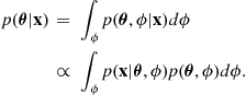
![]() may be calculated in principle by integration:
may be calculated in principle by integration:
![]() (4.12)
(4.12)
and this effectively serves as the normalizing constant for the posterior density (in this and subsequent results the integration would be replaced by a summation in the case of a discrete random vector ![]() ).
).
It is worth reiterating at this stage that we are here implicitly conditioning in this framework on many pieces of additional prior information beyond just the prior parameters of the model ![]() . For example, we are assuming a precise form for the data generation process in the model; if the linear Gaussian model is assumed, then the whole data generation process must follow the probability law of that model, otherwise we cannot guarantee the quality of our answers; the same argument applies to ML estimation, although in the Bayesian setting the distributional form of the Bayesian prior must be assumed in addition. Some texts therefore adopt a notation
. For example, we are assuming a precise form for the data generation process in the model; if the linear Gaussian model is assumed, then the whole data generation process must follow the probability law of that model, otherwise we cannot guarantee the quality of our answers; the same argument applies to ML estimation, although in the Bayesian setting the distributional form of the Bayesian prior must be assumed in addition. Some texts therefore adopt a notation ![]() for Bayesian posterior distributions, where
for Bayesian posterior distributions, where ![]() denotes all of the additional modeling and distributional assumptions that are being made. We will omit this convention for the sake of notational simplicity. However, it will be partially reintroduced when we augment a model with other terms such as unknown hyperparameters (such as
denotes all of the additional modeling and distributional assumptions that are being made. We will omit this convention for the sake of notational simplicity. However, it will be partially reintroduced when we augment a model with other terms such as unknown hyperparameters (such as ![]() in the linear Gaussian model) or a model index
in the linear Gaussian model) or a model index ![]() , when we are considering several competing models (and associated prior distributions) for explaining the data. In these cases, for example, the notation will be naturally extended as required, e.g.,
, when we are considering several competing models (and associated prior distributions) for explaining the data. In these cases, for example, the notation will be naturally extended as required, e.g., ![]() or
or ![]() in the two cases just described.
in the two cases just described.
3.04.2.3.1 Posterior inference and Bayesian cost functions
The posterior distribution gives the probability for any chosen ![]() given observed data
given observed data ![]() , and as such optimally combines our prior information about
, and as such optimally combines our prior information about ![]() and any additional information gained about
and any additional information gained about ![]() from observing
from observing ![]() . We may in principle manipulate the posterior density to infer any required statistic of
. We may in principle manipulate the posterior density to infer any required statistic of ![]() conditional upon
conditional upon ![]() . This is a significant advantage over ML and least squares methods which strictly give us only a single estimate of
. This is a significant advantage over ML and least squares methods which strictly give us only a single estimate of ![]() , known as a “point estimate.” However, by producing a posterior PDF with values defined for all
, known as a “point estimate.” However, by producing a posterior PDF with values defined for all ![]() the Bayesian approach gives a fully interpretable probability distribution. In principle this is as much as one could ever need to know about the inference problem. In signal processing problems, however, we usually require a single point estimate for
the Bayesian approach gives a fully interpretable probability distribution. In principle this is as much as one could ever need to know about the inference problem. In signal processing problems, however, we usually require a single point estimate for ![]() , and a suitable way to choose this is via a “cost function”
, and a suitable way to choose this is via a “cost function” ![]() which expresses objectively a measure of the cost associated with a particular parameter estimate
which expresses objectively a measure of the cost associated with a particular parameter estimate ![]() when the true parameter is
when the true parameter is ![]() (see e.g., [3,6,7]). The form of cost function will depend on the requirements of a particular problem. A cost of 0 indicates that the estimate is perfect for our requirements (this does not necessarily imply that
(see e.g., [3,6,7]). The form of cost function will depend on the requirements of a particular problem. A cost of 0 indicates that the estimate is perfect for our requirements (this does not necessarily imply that ![]() , though it usually will) while positive values indicate poorer estimates. The risk associated with a particular estimator is then defined as the expected posterior cost associated with that estimate:
, though it usually will) while positive values indicate poorer estimates. The risk associated with a particular estimator is then defined as the expected posterior cost associated with that estimate:
![]() (4.13)
(4.13)
We require the estimation scheme which chooses ![]() in order to minimize the risk. The minimum risk is known as the “Bayes risk.” For non-negative cost functions it is sufficient to minimize only the inner integral
in order to minimize the risk. The minimum risk is known as the “Bayes risk.” For non-negative cost functions it is sufficient to minimize only the inner integral
![]() (4.14)
(4.14)
for all ![]() . Typical cost functions are the quadratic cost function
. Typical cost functions are the quadratic cost function ![]() and the uniform cost function, defined for arbitrarily small
and the uniform cost function, defined for arbitrarily small ![]() as
as
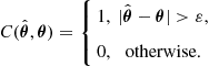 (4.15)
The quadratic cost function leads to the minimum mean-squared error (MMSE)estimator and as such is reasonable for many examples of parameter estimation, where we require an estimate representative of the whole posterior density. To see the form of the resulting estimator, consider differentiation under the integral:

And hence at the optimum estimator we have that the MMSE estimate equals the mean of the posterior distribution:
![]() (4.16)
(4.16)
Where the posterior distribution is symmetrical about its mean the posterior mean can in fact be shown to be the minimum risk solution for any cost function which is a convex function of ![]() [8]. Thus the posterior mean estimator is very often used as the “standard” Bayesian estimate of a parameter. It always needs to be remembered however that there is a whole posterior distribution of parameters available here and that at the very least posterior uncertainty should be summarized through the covariance of the posterior distribution, or posterior standard deviations for the individual elements of the parameter vector. It should be noted as well that in cases where the posterior distribution is multi-modal, that is there is more than one maximum to
[8]. Thus the posterior mean estimator is very often used as the “standard” Bayesian estimate of a parameter. It always needs to be remembered however that there is a whole posterior distribution of parameters available here and that at the very least posterior uncertainty should be summarized through the covariance of the posterior distribution, or posterior standard deviations for the individual elements of the parameter vector. It should be noted as well that in cases where the posterior distribution is multi-modal, that is there is more than one maximum to ![]() , the posterior mean can give very misleading results.
, the posterior mean can give very misleading results.
The uniform cost function on the other hand is useful for the “all or nothing” scenario where we wish to attain the correct parameter estimate at all costs and any other estimate is of no use. Therrien [2] cites the example of a pilot landing a plane on an aircraft carrier. If he does not estimate within some small finite error he misses the ship, in which case the landing is a disaster. The uniform cost function for ![]() leads to the maximum a posteriori (MAP) estimate, the value of
leads to the maximum a posteriori (MAP) estimate, the value of ![]() which maximizes the posterior distribution:
which maximizes the posterior distribution:
![]() (4.17)
(4.17)
Maximum a posteriori (MAP) estimator.
Note that for Gaussian posterior distributions the MMSE and MAP solutions coincide, as indeed they do for any distribution symmetric about its mean with its maximum at the mean.
We now work through the MAP estimation scheme under the linear Gaussian model (4.1). Suppose that the prior on parameter vector ![]() is the multivariate Gaussian (4.71):
is the multivariate Gaussian (4.71):
![]() (4.18)
(4.18)
where ![]() is the prior parameter mean vector,
is the prior parameter mean vector, ![]() is the parameter covariance matrix and P is the number of parameters in
is the parameter covariance matrix and P is the number of parameters in ![]() . If the likelihood
. If the likelihood ![]() takes the same form as before (4.8), the posterior distribution is as follows:
takes the same form as before (4.8), the posterior distribution is as follows:
 (4.19)
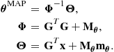
and the MAP estimate ![]() is obtained by differentiation of the log-posterior and finding its unique maximizer as:
is obtained by differentiation of the log-posterior and finding its unique maximizer as:
![]() (4.20)
(4.20)
MAP estimator—linear Gaussian model.
In this expression we can clearly see the “regularizing” effect of the prior density on the ML estimate of (4.9). As the prior becomes more “diffuse,” i.e., the diagonal elements of ![]() increase both in magnitude and relative to the off-diagonal elements, we impose “less” prior information on the estimate. In the limit the prior tends to a uniform (“flat”) prior with all
increase both in magnitude and relative to the off-diagonal elements, we impose “less” prior information on the estimate. In the limit the prior tends to a uniform (“flat”) prior with all ![]() equally probable. In this limit
equally probable. In this limit ![]() and the estimate is identical to the ML estimate (4.9). This useful relationship demonstrates that the ML estimate may be interpreted as the MAP estimate with a uniform prior assigned to
and the estimate is identical to the ML estimate (4.9). This useful relationship demonstrates that the ML estimate may be interpreted as the MAP estimate with a uniform prior assigned to ![]() . The MAP estimate will also tend towards the ML estimate when the likelihood is strongly “peaked” around its maximum compared with the prior. Once again the prior will then have little influence on the shape of the posterior density. It is in fact well known [5] that as the sample size N tends to infinity the Bayes solution tends to the ML solution. This of course says nothing about small sample parameter estimates where the effect of the prior may be very significant.
. The MAP estimate will also tend towards the ML estimate when the likelihood is strongly “peaked” around its maximum compared with the prior. Once again the prior will then have little influence on the shape of the posterior density. It is in fact well known [5] that as the sample size N tends to infinity the Bayes solution tends to the ML solution. This of course says nothing about small sample parameter estimates where the effect of the prior may be very significant.
The choice of a multivariate Gaussian prior may well be motivated by physical considerations about the problem, or it may be motivated by subjective prior knowledge about the value of ![]() (before the data
(before the data ![]() are seen!) in terms of a rough value
are seen!) in terms of a rough value ![]() and a confidence in that value through the covariance matrix
and a confidence in that value through the covariance matrix ![]() (a “subjective” prior). In fact the choice of Gaussian also has the very special property that it makes the Bayesian calculations straightforward and available in closed form. Such a prior is known as a “conjugate” prior [3].
(a “subjective” prior). In fact the choice of Gaussian also has the very special property that it makes the Bayesian calculations straightforward and available in closed form. Such a prior is known as a “conjugate” prior [3].
3.04.2.3.2 Posterior distribution for parameters in the linear Gaussian model
Reconsidering the form of (4.19), we can obtain a lot more information than simply the MAP estimate of (4.20). A fully Bayesian analysis of the problem will study the whole posterior distribution for the unknowns, computing measures of uncertainty, confidence intervals, and so on. The required distribution can be obtained by rearranging the exponent of (4.19) using the result of (4.74),
 (4.21)
![]() (4.22)
(4.22)
![]() (4.23)
(4.23)
![]() (4.24)
(4.24)
Now we can observe that the first term in (4.21), ![]() , is in exactly the correct form for the exponent of a multivariate Gaussian, see (4.71), with mean vector and covariance matrix as follows:
, is in exactly the correct form for the exponent of a multivariate Gaussian, see (4.71), with mean vector and covariance matrix as follows:
![]()
Since the remaining terms in (4.21) do not depend on ![]() , and we know that the multivariate density function must be proper (i.e., integrate to 1), we can conclude that the posterior distribution is itself a multivariate Gaussian,
, and we know that the multivariate density function must be proper (i.e., integrate to 1), we can conclude that the posterior distribution is itself a multivariate Gaussian,
![]() (4.25)
(4.25)
This result will be fundamental for the construction of inference methods in later sections, in cases where the model is at least partially linear/Gaussian, or can be approximated as linear and Gaussian.
3.04.2.3.3 Marginal likelihood
In problems where model choice or classification are of importance, and in inference algorithms which marginalize (“Rao-Blackwellize”) a Gaussian parameter (see later sections for details of these approaches) it will be required to compute the marginal likelihood for the data, i.e.,
![]() (4.26)
(4.26)
Now, filling in the required density functions for the linear Gaussian case, we have:
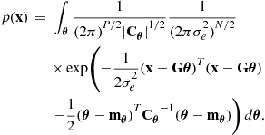 (4.27)
This multivariate Gaussian integral can be performed after some rearrangement using result (4.76) to give:
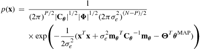 (4.28)
with terms defined exactly as for the posterior distribution calculation above in (4.22)–(4.24).
3.04.2.3.4 Hyperparameters and marginalization of unwanted parameters
In many cases we can formulate a likelihood function for a particular problem which depends on more unknown parameters than are actually wanted for estimation. These will often be “scale” parameters such as unknown noise or excitation variances but may also be unobserved (“missing”) data values or unwanted system parameters. A simple example of such a parameter is ![]() in the linear Gaussian model above. In this case we can directly express the likelihood function exactly as before, but now explicitly conditioning on the unknown noise standard deviation:
in the linear Gaussian model above. In this case we can directly express the likelihood function exactly as before, but now explicitly conditioning on the unknown noise standard deviation:

A full ML procedure requires that the likelihood be maximized w.r.t. all of these parameters and the unwanted values are then simply discarded to give the required estimate, a “concentrated likelihood” estimate.2
However, this may not in general be an appropriate procedure for obtaining only the required parameters—a cost function which depends only upon a certain subset of parameters leads to an estimator which only depends upon the marginal probability for those parameters. The Bayesian approach allows for the interpretation of these unwanted or “nuisance” parameters as random variables, for which as usual we can specify prior densities. If the (possibly multivariate) hyperparameters are ![]() (
(![]() would be taken to equal
would be taken to equal ![]() in the above simple example) then the full model can be specified through a joint prior on the parameters/hyperparameters and the joint likelihood:
in the above simple example) then the full model can be specified through a joint prior on the parameters/hyperparameters and the joint likelihood:
![]()
where the joint prior has been factored using probability chain rule in a way that is often convenient for specification and calculation.
The marginalisation identity can be used to eliminate these parameters from the posterior distribution, and from this we are able to obtain a posterior distribution in terms of only the desired parameters. Consider an unwanted parameter ![]() which is present in the modeling assumptions. The unwanted parameter is now eliminated from the posterior expression by marginalisation:
which is present in the modeling assumptions. The unwanted parameter is now eliminated from the posterior expression by marginalisation:
 (4.29)
3.04.2.3.5 Hyperparameters for the linear Gaussian model
As indicated above, it will often be important to estimate or marginalize the unknown hyperparameters of the linear Gaussian model. There is quite a lot that can be done in the special case of the linear Gaussian model using analytic results. Studying the form of the likelihood function in (4.8), it can be observed that the form of the likelihood is quite similar to that of an inverted-gamma distribution, when considered as a function of ![]() , see Section A.4. This gives a hint as to a possible prior structure that might be workable in this model. If we take the prior itself for
, see Section A.4. This gives a hint as to a possible prior structure that might be workable in this model. If we take the prior itself for ![]() to be inverted-gamma (IG) then it is fairly straightforward to rearrange the conditional posterior distribution for
to be inverted-gamma (IG) then it is fairly straightforward to rearrange the conditional posterior distribution for ![]() into a tractable form. Since we are now treating
into a tractable form. Since we are now treating ![]() as an unknown, conditioning of all terms on this unknown is now made explicit:
as an unknown, conditioning of all terms on this unknown is now made explicit:
 (4.30)
and initially we take ![]() to be independent of
to be independent of ![]() so that
so that ![]() and
and
![]()
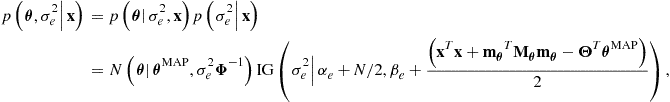
Taking the IG prior ![]() , the conditional probability becomes
, the conditional probability becomes
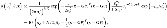 (4.31)
where the equality on the last line follows because we know that the posterior conditional distribution is a proper (normalized) density function, following similar reasoning to the Gaussian posterior distribution leading to (4.25). The IG prior is once again the conjugate prior for the scale parameter ![]() in the model: the posterior distribution is in the same form as the prior distribution, with parameters updated to include the effect of the data (through the likelihood function). This conditional posterior distribution can then be employed later for construction of efficient Gibbs sampling, expectation-maximization, variational Bayes and particle filtering solutions to models involving linear Gaussian components.
in the model: the posterior distribution is in the same form as the prior distribution, with parameters updated to include the effect of the data (through the likelihood function). This conditional posterior distribution can then be employed later for construction of efficient Gibbs sampling, expectation-maximization, variational Bayes and particle filtering solutions to models involving linear Gaussian components.
3.04.2.3.6 Normal-inverted-gamma prior
If a little more structure is included in the prior ![]() then still more can be done analytically. We retain the Gaussian and IG forms for the individual components, but introduce prior dependence between the parameters. Specifically, let
then still more can be done analytically. We retain the Gaussian and IG forms for the individual components, but introduce prior dependence between the parameters. Specifically, let
![]()
where ![]() is a positive definite matrix, considered fixed and known. Here then we are saying that the prior covariance of
is a positive definite matrix, considered fixed and known. Here then we are saying that the prior covariance of ![]() is known up to a scale factor of
is known up to a scale factor of ![]() . The joint prior is then:
. The joint prior is then:
![]()
which is of normal-inverted-gamma form, see (4.83).
Inserting the joint prior into the expression for joint posterior distribution in a similar way to the simple Gaussian prior model for ![]() alone,
alone,
![]()
we obtain as an extension of (4.19),
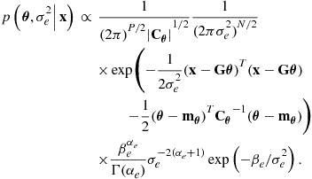 (4.32)
This joint distribution must factor, by the probability chain rule, into:
![]()
The second term in this can be obtained directly from previous results since
![]()
but we already have the first term ![]() in the marginal likelihood calculation of (4.28), now though making the dependence on
in the marginal likelihood calculation of (4.28), now though making the dependence on ![]() explicit and substituting the form
explicit and substituting the form ![]() , so
, so
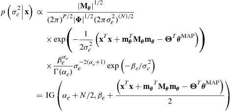
with appropriately simplified terms taken from (4.22)–(4.24) and substituting the form ![]() :
:
It can then be seen by inspection that all of the ![]() terms in may be grouped together in (4.32) as for the Gaussian model to give the remaining required conditional,
terms in may be grouped together in (4.32) as for the Gaussian model to give the remaining required conditional,
![]() (4.33)
(4.33)
Multiplying these two conditionals back together we obtain:
which is in normal-inverted-gamma form—once again, the normal-inverted-gamma prior is conjugate to the linear Gaussian model with unknown linear parameters and noise variance.
The marginal likelihood can also be computed for this model, which will be required for Rao-Blackwellized inference schemes and for model choice problems,
![]() (4.34)
(4.34)
where the first term in this integrand has already been obtained from (4.28), once again with appropriately simplified terms taken from (4.22)–(4.24) and substituting the form ![]() :
:

Now, substituting this back into (4.34), the integral can be completed using the integral result from (4.78),

Despite the advantage of its analytic structure, an obvious challenge of this prior structure is how to specify the matrix ![]() . It can be chosen as some constant
. It can be chosen as some constant ![]() times the identity matrix in the absence of further information, in which case
times the identity matrix in the absence of further information, in which case ![]() can be interpreted as a “parameter-to-noise-ratio” term in the model. This could still be hard to specify in practice without unduly biasing results. One commonly used version of the general structure is the G-prior, which has an interpretation as a signal-to-noise ratio specification.
can be interpreted as a “parameter-to-noise-ratio” term in the model. This could still be hard to specify in practice without unduly biasing results. One commonly used version of the general structure is the G-prior, which has an interpretation as a signal-to-noise ratio specification.
3.04.2.3.7 G-prior
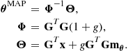
A commonly used form of the above normal-inverted-gamma prior structure is the so-called G-prior, proposed by Zellner [11]. In this, the matrix ![]() is set as follows:
is set as follows:
![]()
where now g is a fixed tuning parameter of the model and has the intuitively appealing interpretation as a prior “signal-to-noise ratio” between the “signal” term ![]() and the “noise” term
and the “noise” term ![]() .
.
The algebra for this prior follows through exactly as for the general case, but with further simplifications. For example, the marginal likelihood becomes
![]()
with
The G-prior has been found to have useful properties for use in model choice problems.
3.04.2.3.8 Priors on covariance matrices
So far in the Bayesian linear Gaussian model no attempt has been made to model correlated structures, either in the noise ![]() or the parameters
or the parameters ![]() , other than through the specification of the covariance matrix of the parameters,
, other than through the specification of the covariance matrix of the parameters, ![]() , which thus far has fixed value or well defined structure (the normal-inverse-gamma model). It is perfectly possible however to assign priors to full covariance matrices and integrate out the matrix as a hyperparameter, or derive its posterior distribution, as required of the particular application. In the linear Gaussian model this principle can be applied to the covariance matrix of the noise term (so far considered to be proportional to the identity matrix, corresponding to independent noise), and/or to the prior covariance matrix of the parameters
, which thus far has fixed value or well defined structure (the normal-inverse-gamma model). It is perfectly possible however to assign priors to full covariance matrices and integrate out the matrix as a hyperparameter, or derive its posterior distribution, as required of the particular application. In the linear Gaussian model this principle can be applied to the covariance matrix of the noise term (so far considered to be proportional to the identity matrix, corresponding to independent noise), and/or to the prior covariance matrix of the parameters ![]() . Take this latter case as an example. We will wish to find an appropriate prior over positive definite matrices that has some tractable properties. In fact, remarkably, there is a conjugate prior for this case which gives full tractability in the linear Gaussian model. This is the inverse Wishart distribution, see Section A.7.
. Take this latter case as an example. We will wish to find an appropriate prior over positive definite matrices that has some tractable properties. In fact, remarkably, there is a conjugate prior for this case which gives full tractability in the linear Gaussian model. This is the inverse Wishart distribution, see Section A.7.
The prior for ![]() would then be:
would then be:
![]()
The full conditional distribution under the linear Gaussian model is obtained in a similar way to the IG prior applied to ![]() in (4.31):
in (4.31):
 (4.35)
where the simplification in the final line is owing to the fact that ![]() is the likelihood function, and does not depend upon
is the likelihood function, and does not depend upon ![]() , and the fact that the prior on
, and the fact that the prior on ![]() does not depend on
does not depend on ![]() , i.e.,
, i.e., ![]() .
.
Now, substituting in the Gaussian and IWi prior terms here from (4.18) and (4.85) we have
 (4.36)
and we can see once again that the inverse Wishart prior is conjugate to the multivariate normal with unknown covariance matrix. Here the result ![]() for column vectors
for column vectors ![]() and
and ![]() has been used to group together the exponent terms in the expression into a single trace expression.
has been used to group together the exponent terms in the expression into a single trace expression.
3.04.2.4 Model uncertainty and Bayesian decision theory
In many problems of practical interest there are also issues of model choice and model uncertainty involved. For example, how can one choose the number of basis functions P in the linear model (4.1)? This could amount for example to a choice of how many sinusoids are necessary to model a given signal, or how many coefficients are required in an autoregressive model formulation. These questions should be answered automatically from the data and can as before include any known prior information about the models. There are a number of frequentist approaches to model choice, typically involving computation of the maximum likelihood parameter vector in each possible model order and then penalizing the likelihood function to prevent over-fitting by inappropriately high model orders. Such standard techniques include the AIC, MDL, and BIC procedures [12], which are typically based on asymptotic and information-theoretic considerations. In the fully Bayesian approach we aim to determine directly the posterior probability for each candidate model. An implicit assumption of the approach is that the true model which generated the data lies within the set of possible candidates; this is clearly an idealization for most real-world problems.
As for Bayesian parameter estimation, we consider the unobserved variable (in this case the model ![]() ) as being generated by some random process whose prior probabilities are known. These prior probabilities are assigned to each of the possible model states using a probability mass function (PMF)
) as being generated by some random process whose prior probabilities are known. These prior probabilities are assigned to each of the possible model states using a probability mass function (PMF) ![]() , which expresses the prior probability of occurrence of different states given all information available except the data
, which expresses the prior probability of occurrence of different states given all information available except the data ![]() . The required form of Bayes’ theorem for this discrete estimation problem is then
. The required form of Bayes’ theorem for this discrete estimation problem is then
![]() (4.37)
(4.37)
![]() is constant for any given
is constant for any given ![]() and will serve to normalize the posterior probabilities over all i in the same way that the marginal likelihood, or “evidence,” normalized the posterior parameter distribution (4.10). In the same way that Bayes rule gave a posterior distribution for parameters
and will serve to normalize the posterior probabilities over all i in the same way that the marginal likelihood, or “evidence,” normalized the posterior parameter distribution (4.10). In the same way that Bayes rule gave a posterior distribution for parameters ![]() , this expression gives the posterior probability for a particular model given the observed data
, this expression gives the posterior probability for a particular model given the observed data ![]() . It would seem reasonable to choose the model
. It would seem reasonable to choose the model ![]() corresponding to maximum posterior probability as our estimate for the true state (we will refer to this state estimate as the MAP estimate), and this can be shown to have the desirable property of minimum classification error rate
corresponding to maximum posterior probability as our estimate for the true state (we will refer to this state estimate as the MAP estimate), and this can be shown to have the desirable property of minimum classification error rate ![]() (see e.g., [7]), that is, it has minimum probability of choosing the wrong model. Note that determination of the MAP model estimate will usually involve an exhaustive search of
(see e.g., [7]), that is, it has minimum probability of choosing the wrong model. Note that determination of the MAP model estimate will usually involve an exhaustive search of ![]() for all feasible i.
for all feasible i.
These ideas are formalized by consideration of a “loss function” ![]() which defines the penalty incurred by taking action
which defines the penalty incurred by taking action ![]() when the true state is
when the true state is ![]() . Action
. Action ![]() will usually refer to the action of choosing model
will usually refer to the action of choosing model ![]() as the estimate.
as the estimate.
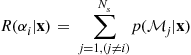
The expected risk associated with action ![]() (known as the conditional risk) is then expressed as
(known as the conditional risk) is then expressed as
 (4.38)
where ![]() is the total number of models under consideration. It can be shown that it is sufficient to minimize this conditional risk in order to achieve the optimal decision rule for a given problem and loss function.
is the total number of models under consideration. It can be shown that it is sufficient to minimize this conditional risk in order to achieve the optimal decision rule for a given problem and loss function.
Consider a loss function which is zero when ![]() and unity otherwise. This “symmetric” loss function can be viewed as the equivalent of the uniform cost function used for parameter estimation (4.15). The conditional risk is then given by:
and unity otherwise. This “symmetric” loss function can be viewed as the equivalent of the uniform cost function used for parameter estimation (4.15). The conditional risk is then given by:
 (4.39)
![]() (4.40)
(4.40)
The second line here is simply the conditional probability that action ![]() is incorrect, and hence minimization of the conditional risk is equivalent to minimization of the probability of classification error,
is incorrect, and hence minimization of the conditional risk is equivalent to minimization of the probability of classification error, ![]() . It is clear from this expression that selection of the MAP state is the optimal decision rule for the symmetric loss function.
. It is clear from this expression that selection of the MAP state is the optimal decision rule for the symmetric loss function.
3.04.2.4.1 Calculation of the marginal likelihood, 
The term ![]() is equivalent to the marginal likelihood term
is equivalent to the marginal likelihood term ![]() which was encountered in the parameter estimation section, since
which was encountered in the parameter estimation section, since ![]() was implicitly conditioned on a particular model structure or state in that scheme.
was implicitly conditioned on a particular model structure or state in that scheme.
If one uses a uniform model prior ![]() , then, according to Eq. (4.37), it is only necessary to compare values of
, then, according to Eq. (4.37), it is only necessary to compare values of ![]() for model selection since the remaining terms are constant for all models.
for model selection since the remaining terms are constant for all models. ![]() can then be viewed literally as the relative “evidence” for a particular model, and two candidate models can be compared through their Bayes Factor:
can then be viewed literally as the relative “evidence” for a particular model, and two candidate models can be compared through their Bayes Factor:
![]()
Typically each model or state ![]() will be expressed in a parametric form whose parameters
will be expressed in a parametric form whose parameters ![]() are unknown. As for the parameter estimation case it will usually be possible to obtain the state conditional parameter likelihood
are unknown. As for the parameter estimation case it will usually be possible to obtain the state conditional parameter likelihood ![]() . Given a model-dependent prior distribution for
. Given a model-dependent prior distribution for ![]() the marginal likelihood may be obtained by integration to eliminate
the marginal likelihood may be obtained by integration to eliminate ![]() from the joint probability
from the joint probability ![]() . The marginal likelihood is then obtained using result (4.29) as
. The marginal likelihood is then obtained using result (4.29) as
![]() (4.41)
(4.41)
If the linear Gaussian model of (4.1) is extended to the multi-model scenario we obtain:
![]() (4.42)
(4.42)
where ![]() refers to the state-dependent basis matrix and
refers to the state-dependent basis matrix and ![]() is the corresponding error sequence. For this model the state dependent parameter likelihood
is the corresponding error sequence. For this model the state dependent parameter likelihood ![]() is (see (4.8)):
is (see (4.8)):
 (4.43)
If we for example take the same Gaussian form for the state conditional parameter prior ![]() (with
(with ![]() parameters) as we used for
parameters) as we used for ![]() in (4.18) the marginal likelihood is then given with minor modification as:
in (4.18) the marginal likelihood is then given with minor modification as:
 (4.44)
with terms defined as
![]() (4.45)
(4.45)
![]() (4.46)
(4.46)
![]() (4.47)
(4.47)
Notice that ![]() is simply the model-dependent version of the MAP parameter estimate given by (4.20). We can also of course look at the more sophisticated models using normal-inverted-gamma priors or G-priors, as before, and then the marginal likelihood expressions are again as given for the parameter estimation case.
is simply the model-dependent version of the MAP parameter estimate given by (4.20). We can also of course look at the more sophisticated models using normal-inverted-gamma priors or G-priors, as before, and then the marginal likelihood expressions are again as given for the parameter estimation case.
3.04.2.5 Structures for model uncertainty
Model uncertainty may often be expressed in a highly structured way: in particular the models may be nested or subset structures. In the nested structure for the linear model, the basis matrix for model ![]() is obtained by adding an additional basis vector to the
is obtained by adding an additional basis vector to the ![]() :
:
![]()
and hence the model of higher order inherits part of its structure from the lower order models. In subset, or “variable selection” models, a (potentially very large) pool of basis vectors ![]() is available for construction of the model, and each candidate model is composed by taking a specific subset of the available vectors. A particular model
is available for construction of the model, and each candidate model is composed by taking a specific subset of the available vectors. A particular model ![]() is then specified by a set of
is then specified by a set of ![]() distinct integer indices
distinct integer indices ![]() and the
and the ![]() matrix is constructed as
matrix is constructed as
![]()
In such a case there are ![]() possible subset models, which could be a huge number. Very often it will be infeasible to explore the posterior probabilities of all possible subsets, and hence sub-optimal search strategies are adopted, such as the MCMC algorithms of [13].
possible subset models, which could be a huge number. Very often it will be infeasible to explore the posterior probabilities of all possible subsets, and hence sub-optimal search strategies are adopted, such as the MCMC algorithms of [13].
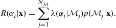
3.04.2.6 Bayesian model averaging
In many scenarios where there is model uncertainty, model choice is not the primary aim of the inference. Take for example the case where a state vector ![]() is common to all models, but each model has different parameters
is common to all models, but each model has different parameters ![]() , and the observed data are
, and the observed data are ![]() . Then the correct Bayesian procedure for inference about
. Then the correct Bayesian procedure for inference about ![]() is to perform marginalisation over all possible models, or perform Bayesian model averaging (BMA):
is to perform marginalisation over all possible models, or perform Bayesian model averaging (BMA):
![]()
Note though that ![]() and
and ![]() may not be analytically computable since they both require marginalizations (over
may not be analytically computable since they both require marginalizations (over ![]() and/or
and/or ![]() ) and in these cases numerical strategies such as Markov chain Monte Carlo (MCMC) would be required.
) and in these cases numerical strategies such as Markov chain Monte Carlo (MCMC) would be required.
3.04.3 Computational methods
In previous sections we have considered the basic frameworks for Bayesian inference, illustrated through the linear Gaussian model. This model makes many of the required calculations straightforward and analytically computable. However, for most real-world problems there will nearly always be intractable elements in the models, and for these numerical Bayesian methods are required. Take for example the sinusoidal model presented earlier. If we make the frequencies ![]() unknown then the model is highly non-linear in these parameters. Similarly with the autoregressive model, if the signal is now observed in noise
unknown then the model is highly non-linear in these parameters. Similarly with the autoregressive model, if the signal is now observed in noise ![]() as
as
![]()
then the posterior distribution for the parameters is no longer obtainable in closed form.
There is a wide range of computational tools now available for solving complex Bayesian inference problems, ranging from simple Laplace approximations to posterior densities, through variational Bayes methods to highly sophisticated Monte Carlo schemes. We will only attempt to give a flavor of some of the techniques out there, starting with one of the simplest and most effective: the EM algorithm.
3.04.3.1 Expectation-maximization (EM) for MAP estimation
The expectation-maximization (EM) algorithm [14] is an iterative procedure for finding modes of a posterior distribution or likelihood function, particularly in the context of “missing data.” EM has been used quite extensively in the signal processing literature for maximum likelihood parameter estimation, see e.g., [15–18]. The notation used here is essentially similar to that of Tanner [19, pp. 38–57].
The problem is formulated in terms of observed data ![]() , parameters
, parameters ![]() and unobserved (“latent” or “missing”) data
and unobserved (“latent” or “missing”) data ![]() . A prototypical example of such a set-up is the AR model in noise:
. A prototypical example of such a set-up is the AR model in noise:
 (4.48)
![]()
in which the parameters to learn will be ![]() .
.
EM is useful in certain cases where it is straightforward to manipulate the conditional posterior distributions ![]() and
and ![]() , but perhaps not straightforward to deal with the marginal distributions
, but perhaps not straightforward to deal with the marginal distributions ![]() and
and ![]() . The objective of EM in the Bayesian case is to obtain the MAP estimate for parameters:
. The objective of EM in the Bayesian case is to obtain the MAP estimate for parameters:
![]()
The basic Bayesian EM algorithm can be summarized as:

These two steps are iterated until convergence is achieved. The algorithm is guaranteed to converge to a stationary point of ![]() , although we must beware of convergence to local maxima when the posterior distribution is multimodal. The starting point
, although we must beware of convergence to local maxima when the posterior distribution is multimodal. The starting point ![]() determines which posterior mode is reached and can be critical in difficult applications.
determines which posterior mode is reached and can be critical in difficult applications.
EM-based methods can be thought of as a special case of variational Bayes methods [20,21]. In these, typically favoured by the machine learning community, a factored approximation to the joint posterior density is constructed, and each factor is iteratively updated using formulae somewhat similar to EM.
3.04.3.2 Markov chain Monte Carlo (MCMC)
At the more computationally expensive end of the spectrum we can consider Markov chain Monte Carlo (MCMC) simulation methods [22,23]. The object of these methods is to draw samples from some target distribution ![]() which may be too complex for direct estimation procedures. The MCMC approach sets up an irreducible, aperiodic Markov chain whose stationary distribution is the target distribution of interest,
which may be too complex for direct estimation procedures. The MCMC approach sets up an irreducible, aperiodic Markov chain whose stationary distribution is the target distribution of interest, ![]() . The Markov chain is then simulated from some arbitrary starting point and convergence in distribution to
. The Markov chain is then simulated from some arbitrary starting point and convergence in distribution to ![]() is then guaranteed under mild conditions as the number of state transitions (iterations) approaches infinity [24]. Once convergence is achieved, subsequent samples from the chain form a (dependent) set of samples from the target distribution, from which Monte Carlo estimates of desired quantities related to the distribution may be calculated.
is then guaranteed under mild conditions as the number of state transitions (iterations) approaches infinity [24]. Once convergence is achieved, subsequent samples from the chain form a (dependent) set of samples from the target distribution, from which Monte Carlo estimates of desired quantities related to the distribution may be calculated.
For the statistical models considered in this chapter, the target distribution will be the joint posterior distribution for all unknowns, ![]() , from which samples of the unknowns
, from which samples of the unknowns ![]() and
and ![]() will be drawn conditional upon the observed data
will be drawn conditional upon the observed data ![]() . Since the joint distribution can be factorised as
. Since the joint distribution can be factorised as ![]() it is clear that the samples in
it is clear that the samples in ![]() which are extracted from the joint distribution are equivalent to samples from the marginal posterior
which are extracted from the joint distribution are equivalent to samples from the marginal posterior ![]() . The sampling method thus implicitly performs the (generally) analytically intractable marginalisation integral w.r.t.
. The sampling method thus implicitly performs the (generally) analytically intractable marginalisation integral w.r.t. ![]() .
.
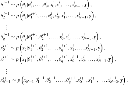
The Gibbs Sampler [25,26] is perhaps the most simple and popular form of MCMC currently in use for the exploration of posterior distributions. This method, which can be derived as a special case of the more general Metropolis-Hastings method [22], requires the full specification of conditional posterior distributions for each unknown parameter or variable. Suppose that the reconstructed data and unknown parameters are split into (possibly multivariate) subsets ![]() and
and ![]() . Arbitrary starting values
. Arbitrary starting values ![]() and
and ![]() are assigned to the unknowns. A single iteration of the Gibbs Sampler then comprises sampling each variable from its conditional posterior with all remaining variables fixed to their current sampled value. The
are assigned to the unknowns. A single iteration of the Gibbs Sampler then comprises sampling each variable from its conditional posterior with all remaining variables fixed to their current sampled value. The ![]() th iteration of the sampler may be summarized as:
th iteration of the sampler may be summarized as:
where the notation “![]() ” denotes that the variable to the left is drawn as a random independent sample from the distribution to the right.
” denotes that the variable to the left is drawn as a random independent sample from the distribution to the right.
The utility of the Gibbs Sampler arises as a result of the fact that the conditional distributions, under appropriate choice of parameter and data subsets (![]() and
and ![]() ), will be more straightforward to sample than the full posterior. Multivariate parameter and data subsets can be expected to lead to faster convergence in terms of number of iterations (see e.g., [27,28]), but there may be a trade-off in the extra computational complexity involved per iteration. Convergence properties are a difficult and important issue and concrete results are fairly rare. Numerous (but mostly ad hoc) convergence diagnostics have been devised for more general scenarios and a review may be found in [29], for example.
), will be more straightforward to sample than the full posterior. Multivariate parameter and data subsets can be expected to lead to faster convergence in terms of number of iterations (see e.g., [27,28]), but there may be a trade-off in the extra computational complexity involved per iteration. Convergence properties are a difficult and important issue and concrete results are fairly rare. Numerous (but mostly ad hoc) convergence diagnostics have been devised for more general scenarios and a review may be found in [29], for example.
Once the sampler has converged to the desired posterior distribution, inference can easily be made from the resulting samples. One useful means of analysis is to form histograms or kernel density estimates of any parameters of interest. These converge in the limit to the true marginal posterior distribution for those parameters and can be used to estimate MAP values and Bayesian confidence intervals, for example. Alternatively a Monte Carlo estimate can be made for the expected value of any desired posterior functional ![]() as a finite summation:
as a finite summation:
![]() (4.51)
(4.51)
where ![]() is the convergence (“burn in”) time and
is the convergence (“burn in”) time and ![]() is the total number of iterations. The MMSE estimator for example, is simply the posterior mean, estimated by setting
is the total number of iterations. The MMSE estimator for example, is simply the posterior mean, estimated by setting ![]() in (4.51).
in (4.51).
MCMC methods are computer-intensive and will only be applicable when off-line processing is acceptable and the problem is sufficiently complex to warrant their sophistication. However, they are currently unparalleled in ability to solve the most challenging of modeling problems. A more extensive survey can be found in the E-reference article by A.T. Cemgil. Further reading material includes MCMC for model uncertainty [30,31].
3.04.4 State-space models and sequential inference
Inthis section we describe inference methods that run sequentially, or on-line, using the state-space formulation. These are vital in many applications, where either the data are too large to process in one batch, or results need to be produced in real-time as new data points arrive. In sequential inference we have seen some of the most exciting advances in methodology over the last decade.
3.04.4.1 Linear Gaussian state-space models
Most linear time series models, including the AR models discussed earlier, can be expressed in the state space form:
![]() (4.52)
(4.52)
![]() (4.53)
(4.53)
In the top line, the observation equation, the observed data ![]() is expressed in terms of an unobserved state
is expressed in terms of an unobserved state ![]() and a noise term
and a noise term ![]() .
. ![]() is uncorrelated (i.e.,
is uncorrelated (i.e., ![]() for
for ![]() ) and zero mean, with covariance
) and zero mean, with covariance ![]() . In the second line, the state update equation,the state
. In the second line, the state update equation,the state ![]() is updated to its new value
is updated to its new value ![]() at time
at time ![]() and a second noise term
and a second noise term ![]() .
. ![]() is uncorrelated (i.e.,
is uncorrelated (i.e., ![]() for
for ![]() ) and zero mean, with covariance
) and zero mean, with covariance ![]() , and is also uncorrelated with
, and is also uncorrelated with ![]() . Note that in general the state
. Note that in general the state ![]() , observation
, observation ![]() and noise terms
and noise terms ![]() /
/![]() can be column vectors and the constants
can be column vectors and the constants ![]() , and H are then matrices of the implied dimensionality. Also note that all of these constants can be made time index dependent without altering the form of the results given below.
, and H are then matrices of the implied dimensionality. Also note that all of these constants can be made time index dependent without altering the form of the results given below.
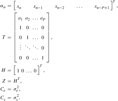
Take, for example, an AR model ![]() observed in noise
observed in noise ![]() ,so that the equations in standard form are:
,so that the equations in standard form are:

One way to express this in state-space form is as follows:
The state-space form is useful since some elegant results exist for the general form which can be applied in many different special cases. In particular, we will use it for sequential estimation of the state ![]() . In probabilistic terms this will involve updating the posterior probability for
. In probabilistic terms this will involve updating the posterior probability for ![]() with the input of a new observation
with the input of a new observation ![]() :
:
![]()
where ![]() and
and ![]() denotes the sequential updating function.
denotes the sequential updating function.
Suppose that the noise sources ![]() and
and ![]() are Gaussian. Assume also that an initial state probability or prior
are Gaussian. Assume also that an initial state probability or prior ![]() exists and is Gaussian
exists and is Gaussian ![]() . Then the posterior distributions are all Gaussian themselves and the posterior distribution for
. Then the posterior distributions are all Gaussian themselves and the posterior distribution for ![]() is fully represented by its sufficient statistics: its mean
is fully represented by its sufficient statistics: its mean ![]() and covariance matrix
and covariance matrix ![]() . TheKalman filter [9,32,33] performs the update efficiently, as follows:
. TheKalman filter [9,32,33] performs the update efficiently, as follows:
Here ![]() is the predictive mean
is the predictive mean ![]() ,
, ![]() the predictive covariance
the predictive covariance ![]() and I denotes the (appropriately sized) identity matrix.
and I denotes the (appropriately sized) identity matrix.
This is the probabilistic interpretation of the Kalman filter, assuming Gaussian distributions for noise sources and initial state, and it is this form that we will require in the next section on sequential Monte Carlo. In that section it will be more fully developed in the probabilistic version. The more standard interpretation is as the best linear estimator for the state [9,32,33].
3.04.4.2 The prediction error decomposition
One remarkable property of the Kalman filter is the prediction error decomposition which allows exact sequential evaluation of the likelihood function for the observations. If we suppose that the model depends upon some hyperparameters ![]() , then the Kalman filter updates sequentially, for a particular value of
, then the Kalman filter updates sequentially, for a particular value of ![]() , the density
, the density ![]() . We define the likelihood for
. We define the likelihood for ![]() in this context to be:
in this context to be:
![]()
from which the ML or MAP estimator for ![]() can be obtained by optimization. The prediction error decomposition [9, pp. 125–126] calculates this term from the outputs of the Kalman filter:
can be obtained by optimization. The prediction error decomposition [9, pp. 125–126] calculates this term from the outputs of the Kalman filter:
![]() (4.54)
(4.54)
where
![]()
3.04.4.3 Sequential Monte Carlo (SMC)
It is now many years since the pioneering contribution of Gordon et al. [34], which is commonly regarded as the first instance of modern sequential Monte Carlo (SMC) approaches. Initially focussed on applications to tracking and vision, these techniques are now very widespread and have had a significant impact in virtually all areas of signal and image processing concerned with Bayesian dynamical models. This section serves as a brief introduction to the methods for the practitioner.
Consider the following generic nonlinear extension of the linear state-space model:
By these equations we mean that the hidden states ![]() and data
and data ![]() are assumed to be generated by nonlinear functions
are assumed to be generated by nonlinear functions ![]() and
and ![]() , respectively, of the state and noise disturbances
, respectively, of the state and noise disturbances ![]() and
and ![]() . The precise form of the functions and the assumed probability distributions of the state
. The precise form of the functions and the assumed probability distributions of the state ![]() and the observation
and the observation ![]() noises imply via a change of variables the transition probability density function
noises imply via a change of variables the transition probability density function ![]() and the observation probability density function
and the observation probability density function ![]() . It is assumed that
. It is assumed that ![]() is Markovian, i.e., its conditional probability density given the past states
is Markovian, i.e., its conditional probability density given the past states ![]() depends only on
depends only on ![]() through the transition density
through the transition density ![]() , and that the conditional probability density of
, and that the conditional probability density of ![]() given the states
given the states ![]() and the past observations
and the past observations ![]() depends only upon
depends only upon ![]() through the conditional likelihood
through the conditional likelihood ![]() . We further assume that the initial state
. We further assume that the initial state ![]() is distributed according to a density function
is distributed according to a density function ![]() . Such nonlinear dynamic systems arise frequently from many areas in science and engineering such as target tracking, computer vision, terrain referenced navigation, finance, pollution monitoring, communications, audio engineering, to list but a few.
. Such nonlinear dynamic systems arise frequently from many areas in science and engineering such as target tracking, computer vision, terrain referenced navigation, finance, pollution monitoring, communications, audio engineering, to list but a few.
A simple and standard example is now given to illustrate the model class.
Example 1
(Nonlinear time series model) This model has been used quite extensively in the filtering literature [34–36]. The required equations are as follows:

where ![]() and
and ![]() and here
and here ![]() and
and ![]() are considered fixed and known;
are considered fixed and known; ![]() once again denotes the normal distribution with mean
once again denotes the normal distribution with mean ![]() and variance
and variance ![]() . The representation in terms of densities
. The representation in terms of densities ![]() and
and ![]() is given by:
is given by:

The form of these densities was straightforward to obtain in this case. For more complex cases a Jacobian term might be required when either ![]() or
or ![]() is a nonlinear function of
is a nonlinear function of ![]() or
or ![]() , respectively.
, respectively.
States may easily be simulated from a dynamical model of this sort owing to the Markovian assumptions on ![]() and
and ![]() , which imply that the joint probability density of states and observations, denoted
, which imply that the joint probability density of states and observations, denoted ![]() , may be factorized as
, may be factorized as

A graphical representation of the dependencies between different states and observations is shown in Figure 4.1.

The ability to simulate random states and to evaluate the transition and observation densities (at least up to an unknown normalizing constant) will be principal components of the particle filtering algorithms described shortly.
Bayesian inference for the general nonlinear dynamic system above involves computing the posterior distribution of a collection of state variables ![]() conditioned on a batch of observations,
conditioned on a batch of observations, ![]() , which we denote
, which we denote ![]() . Specific problems include filtering, for
. Specific problems include filtering, for ![]() , fixed lag smoothing, when
, fixed lag smoothing, when ![]() and fixed interval smoothing, if
and fixed interval smoothing, if ![]() and
and ![]() . Despite the apparent simplicity of the above problem, the posterior distribution can be computed in closed form only in very specific cases, principally, the linear Gaussian model (where the functions
. Despite the apparent simplicity of the above problem, the posterior distribution can be computed in closed form only in very specific cases, principally, the linear Gaussian model (where the functions ![]() and
and ![]() are linear and
are linear and ![]() and
and ![]() are Gaussian) and the discrete hidden Markov model (where
are Gaussian) and the discrete hidden Markov model (where ![]() takes its values in a finite alphabet). In the vast majority of cases, nonlinearity or non-Gaussianity render an analytic solution intractable [32,37–39].
takes its values in a finite alphabet). In the vast majority of cases, nonlinearity or non-Gaussianity render an analytic solution intractable [32,37–39].
There are many classical (non-Monte Carlo-based) methods for nonlinear dynamic systems, including the extended Kalman filter (EKF) and its variants [40], Gaussian sum filters [41], unscented and quadrature Kalman filters [42–44]. However, limitations in the generality of these approaches to the most nonlinear/non-Gaussian systems has stimulated interest in more general techniques. Among these, Monte Carlo methods, in which the posterior distribution is represented by a collection of random points, are central. Early approaches include sequential importance sampling in the pioneering works of Handschin and Mayne [45] and Handschin [46]. The incorporation of resampling techniques was key though to the practical success of such approaches, as given in [34]. Without resampling, as the number of time points increases, the importance weights tend to degenerate, a phenomenon known as sample impoverishment or weight degeneracy. Since then, there have been several independent variants of similar filtering ideas, including the Condensation filter [47], Monte Carlo filter [35], Sequential imputations [48], and the Particle filter [49]. So far, sequential Monte Carlo (SMC) methods have been successfully applied in many different fields including computer vision, signal processing, tracking, control, econometrics, finance, robotics, and statistics; see [37,39,50,51] and the references therein for a good review coverage.
3.04.4.3.1 Predictor-corrector formulation
We now present the basic update for the state-space model. Starting with the initial, or “prior,” distribution ![]() , the posterior density
, the posterior density ![]() can be obtained using the following prediction-correction recursion [52]:
can be obtained using the following prediction-correction recursion [52]:
3.04.4.4 Particle filtering and auxiliary sampling
We now present a general form for of the particle filter, using the auxiliary filtering ideas of Pitt and Shephard [53], and which includes most common variants as special cases. We first represent the posterior smoothing density approximately as a weighted sum of ![]() functions
functions
 (4.59)
where the notation ![]() denotes the Dirac mass at point
denotes the Dirac mass at point ![]() . Under suitable technical assumptions, this is a consistent approximation, i.e., for any function h on the path space
. Under suitable technical assumptions, this is a consistent approximation, i.e., for any function h on the path space

converges to ![]() as the number N of particles increases to infinity, see [37,54–58] for technical considerations.
as the number N of particles increases to infinity, see [37,54–58] for technical considerations.
The formulation given here is equivalent to that given by Pitt and Shephard [53], although we avoid the explicit inclusion of an auxiliary indexing variable by considering a proposal over the entire path of the process up to time t. The starting assumption is that the joint posterior at ![]() is well approximated as
is well approximated as
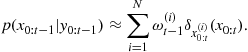
Based on this assumption the joint posterior distribution at time t is approximated by substitution into the prediction-correction equations:
 (4.60)
where the normalization factor Z is given by

Now we consider a general joint proposal for the entire path of the new particles ![]() , that is,
, that is,
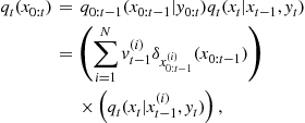
where ![]() and
and ![]() . Notice that the proposal splits into two parts: a marginal proposal
. Notice that the proposal splits into two parts: a marginal proposal ![]() for the past path of the process
for the past path of the process ![]() and a conditional proposal
and a conditional proposal ![]() for the new state
for the new state ![]() . Note that the first component is constructed to depend explicitly on data up to time t in order to allow adaptation of the proposal in the light of the new data point
. Note that the first component is constructed to depend explicitly on data up to time t in order to allow adaptation of the proposal in the light of the new data point ![]() (and indeed it may depend on future data points as well if some look-ahead and latency is allowable). The first part of the proposal is a discrete distribution centered upon the old particle paths
(and indeed it may depend on future data points as well if some look-ahead and latency is allowable). The first part of the proposal is a discrete distribution centered upon the old particle paths ![]() , but now with probability mass for each component in the proposal distribution designed to be
, but now with probability mass for each component in the proposal distribution designed to be ![]() . The weighting function
. The weighting function ![]() can be data dependent, the rationale being that we should preselect particles that are a good fit to the new data point
can be data dependent, the rationale being that we should preselect particles that are a good fit to the new data point ![]() . For example, Pitt and Shephard [53] suggest taking a point value
. For example, Pitt and Shephard [53] suggest taking a point value ![]() of the state, say the mean or mode of
of the state, say the mean or mode of ![]() , and computing the weighting function as the likelihood evaluated at this point, i.e.,
, and computing the weighting function as the likelihood evaluated at this point, i.e., ![]() ; or if the particles from
; or if the particles from ![]() are weighted, one would choose
are weighted, one would choose ![]() .
.
Using this proposal mechanism it is then possible to define an importance ratio between the approximate posterior in (4.60) and the full path proposal q, given by

The choice of the proposal terms ![]() and
and ![]() then determines the behavior of the particle filter. With
then determines the behavior of the particle filter. With ![]() constant and
constant and ![]() set to equal the transition density, we achieve the standard bootstrap filter of [34]. With
set to equal the transition density, we achieve the standard bootstrap filter of [34]. With ![]() constant and
constant and ![]() chosen to be a data-dependent proposal for the new state, we have the particle filter of [59].
chosen to be a data-dependent proposal for the new state, we have the particle filter of [59].
More general schemes that allow some exploration of future data points by so-called pilot sampling to generate the weighting function have been proposed in, for example [60], while further discussion of the framework can be found in [61]. A summary of the auxiliary particle filter is given in Algorithm 1. We assume here that the selection (resampling) step occurs at each point, although it may be omitted exactly as in the standard particle filter, in which case no weight correction is applied. These techniques are developed and extensively reviewed in [37,39,44,59,62,63].
A diagrammatic representation of the bootstrap filter in operation is given in Figure 4.2, in which the resampling (selection) step is seen to concentrate particles (asterisks) into the two high probability modes of the density function.

Figure 4.2 The bootstrap filter in operation from time t to ![]() , nonlinear time series Example 1. Asterisks show the positions of (a small selection of) the particles at each stage. The solid line shows a kernel density estimate of the distributions represented at each stage. Ten thousand particles were used in total. Notice that resampling concentrates particles into the region of high probability.
, nonlinear time series Example 1. Asterisks show the positions of (a small selection of) the particles at each stage. The solid line shows a kernel density estimate of the distributions represented at each stage. Ten thousand particles were used in total. Notice that resampling concentrates particles into the region of high probability.
3.04.4.4.1 Marginalized particle filters
In many practical scenarios, especially those found in the tracking domain, the models are not entirely nonlinear and non-Gaussian. By this we mean that some subset of the state vector is linear and Gaussian, conditional upon the other states. In these cases one may use standard linear Gaussian optimal filtering for the linear part, and particle filtering for the nonlinear part. This may be thought of as an optimal Gaussian mixture approximation to the filtering distribution. See [59,64,65] for detailed descriptions of this approach to the problem, which is referred to either as the Rao-Blackwellized particle filter, or Mixture Kalman filter. Recent work [66,67] has studied in detail the possible classes of model that may be handled by the marginalized filter, and computational complexity issues. The formulation is as follows.3 First, the state is partitioned into two components, ![]() and
and ![]() , referring respectively to the linear (“L”) and nonlinear (“N”) components. The linear part of the model is expressed in the form of a linear Gaussian state-space model as follows, with state-space matrices that may depend upon the nonlinear state
, referring respectively to the linear (“L”) and nonlinear (“N”) components. The linear part of the model is expressed in the form of a linear Gaussian state-space model as follows, with state-space matrices that may depend upon the nonlinear state ![]() :
:

![]() (4.61)
(4.61)
![]() (4.62)
(4.62)
Here ![]() and
and ![]() are independent, zero-mean, Gaussian disturbances with covariances
are independent, zero-mean, Gaussian disturbances with covariances ![]() and
and ![]() , respectively, and
, respectively, and ![]() and
and ![]() are matrices of compatible dimensions that may depend upon the nonlinear state
are matrices of compatible dimensions that may depend upon the nonlinear state ![]() . At
. At ![]() , the linear part of the model is initialised with
, the linear part of the model is initialised with ![]() .
.
Now the nonlinear part of the state obeys a general dynamical model (which is not necessarily Markovian):
![]() (4.63)
(4.63)
In such a case, conditioning on the nonlinear part of the state ![]() and the observations
and the observations ![]() , the linear part of the state is jointly Gaussian and the means and covariances of this Gaussian representation may be obtained by using the classical Kalman filtering recursions [68]. The basic idea is then to marginalize the linear part of the state vector to obtain the posterior distribution of the nonlinear part of the state:
, the linear part of the state is jointly Gaussian and the means and covariances of this Gaussian representation may be obtained by using the classical Kalman filtering recursions [68]. The basic idea is then to marginalize the linear part of the state vector to obtain the posterior distribution of the nonlinear part of the state:
![]()
Particle filtering is then run on the nonlinear state sequence only, with target distribution ![]() . The resulting algorithm is almost exactly as before, requiring only a slight modification to the basic particle filter to allow for the fact that the marginalized system is no longer Markovian, since
. The resulting algorithm is almost exactly as before, requiring only a slight modification to the basic particle filter to allow for the fact that the marginalized system is no longer Markovian, since
![]()
Moreover, the dynamical model for the nonlinear part of the state may itself be non-Markovian, see Eq. (4.63).
Thus, instead of the usual updating rule we have:
![]() (4.64)
(4.64)
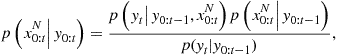 (4.65)
where as before ![]() is the predictive distribution of
is the predictive distribution of ![]() given the past observations
given the past observations ![]() , which is a fixed normalizing constant (independent of the state sequence
, which is a fixed normalizing constant (independent of the state sequence ![]() ).
).
Note that if ![]() denote the particles evolving in the state-space of the nonlinear variables according to the above equations, and their associated importance weights, estimation of the linear part of the state may be done using a Rao-Blackwellized estimation scheme [69]: the posterior density for the linear part is obtained as a random Gaussian mixture approximation given by
denote the particles evolving in the state-space of the nonlinear variables according to the above equations, and their associated importance weights, estimation of the linear part of the state may be done using a Rao-Blackwellized estimation scheme [69]: the posterior density for the linear part is obtained as a random Gaussian mixture approximation given by
 (4.66)
where the conditional densities ![]() are Gaussian and computed again using Kalman filtering recursions. Equation (4.66) replaces the standard point-mass approximation (4.59) arising in the generic particle filter. The Rao-Blackwellized estimate is usually better in terms of Monte Carlo error than the corresponding scheme that performs standard particle filtering jointly in both nonlinear and linear states. The computational trade-off is more complex, however, since the marginalized filter can be significantly more time-consuming than the standard filter per particle. These trade-offs have been extensively studied by Schön et al. [66] and in many cases the performance/computation trade-off comes out in favor of the marginalized filter.
are Gaussian and computed again using Kalman filtering recursions. Equation (4.66) replaces the standard point-mass approximation (4.59) arising in the generic particle filter. The Rao-Blackwellized estimate is usually better in terms of Monte Carlo error than the corresponding scheme that performs standard particle filtering jointly in both nonlinear and linear states. The computational trade-off is more complex, however, since the marginalized filter can be significantly more time-consuming than the standard filter per particle. These trade-offs have been extensively studied by Schön et al. [66] and in many cases the performance/computation trade-off comes out in favor of the marginalized filter.
To give further detail to the approach, we first summarize the Kalman filter itself in this probabilistic setting [52], then we place the whole scheme back in the particle filtering context. As a starting point, assume the distribution ![]() has been obtained. This is a Gaussian, denoted by
has been obtained. This is a Gaussian, denoted by
![]()
where the mean and covariance terms are dependent upon both ![]() and
and ![]() . Now, (4.61) shows how to update this distribution one step, since
. Now, (4.61) shows how to update this distribution one step, since ![]() is just a summation of two transformed independent Gaussian random vectors,
is just a summation of two transformed independent Gaussian random vectors, ![]() and
and ![]() , which itself must be a Gaussian. Under the standard rules for summation of independent Gaussian random vectors, we obtain the predictive distribution for
, which itself must be a Gaussian. Under the standard rules for summation of independent Gaussian random vectors, we obtain the predictive distribution for ![]() , conditioned upon
, conditioned upon ![]() and
and ![]() , as follows:
, as follows:
![]() (4.67)
(4.67)
where

As a second step in the update, the new data point ![]() is incorporated through Bayes’ theorem:
is incorporated through Bayes’ theorem:
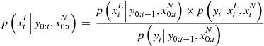 (4.68)
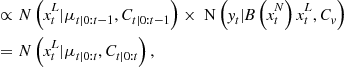
where ![]() and
and ![]() are obtained by standard rearrangement formulae as
are obtained by standard rearrangement formulae as

and where the term ![]() is known as the Kalman Gain. In order to complete the analysis for particle filter use, one further term is required,
is known as the Kalman Gain. In order to complete the analysis for particle filter use, one further term is required, ![]() . This is obtained by the so-called prediction error decomposition, which is easily obtained from (4.67), since
. This is obtained by the so-called prediction error decomposition, which is easily obtained from (4.67), since ![]() is obtained by summing a transformed version of
is obtained by summing a transformed version of ![]() , i.e.,
, i.e., ![]() , with an independent zero-mean Gaussian noise term
, with an independent zero-mean Gaussian noise term ![]() having covariance
having covariance ![]() , leading to:
, leading to:
![]() (4.69)
(4.69)
where

In order to construct the marginalized particle filter, notice that for any realization of the nonlinear state sequence ![]() , and data sequence
, and data sequence ![]() , one may calculate the value of
, one may calculate the value of ![]() in (4.69) through sequential application of the formulae (4.67) and (4.68). The marginalized particle filter then requires computation and storage of the term
in (4.69) through sequential application of the formulae (4.67) and (4.68). The marginalized particle filter then requires computation and storage of the term ![]() in (4.69), for each particle realization
in (4.69), for each particle realization ![]() . In the marginalized particle filter the particles are stored as the nonlinear part of the state
. In the marginalized particle filter the particles are stored as the nonlinear part of the state ![]() , the associated sufficient statistics for each particle, i.e.,
, the associated sufficient statistics for each particle, i.e., ![]() and
and ![]() , and the weight for each particle. We do not give the entire modified algorithm. The only significant change is to the weighting step, which becomes
, and the weight for each particle. We do not give the entire modified algorithm. The only significant change is to the weighting step, which becomes
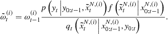
As an important aside, we note that the marginalized filter may also be used to good effect when the linear states are unknown but “static” over time, i.e., ![]() with some Gaussian initial distribution or prior
with some Gaussian initial distribution or prior ![]() , as before. Then the marginalized filter runs exactly as before but we are now able to marginalize, or infer the value of, a static parameter
, as before. Then the marginalized filter runs exactly as before but we are now able to marginalize, or infer the value of, a static parameter ![]() . Early versions of such filters are found in the sequential imputations work of [48], for example.
. Early versions of such filters are found in the sequential imputations work of [48], for example.
We have focused here on the linear Gaussian case of the marginalized filter. However, another important class of models is the discrete state-space hidden Markov model, in which the states are discrete values and switching may occur between one time and the next according to a Markov transition matrix. As for the linear Gaussian case, the discrete state values may be marginalized to form a marginalized particle filter, using the HMM forward algorithm [70] instead of the Kalman filter [59]. For simulations and examples within both frameworks, see [37,59].
As mentioned before, several generalisations are possible to the basic model. The most basic of these allow dependence of the matrices ![]() , and
, and ![]() to depend on time, and any or all elements of the nonlinear state sequence
to depend on time, and any or all elements of the nonlinear state sequence ![]() . None of these changes require any modification to the algorithm formulation. Another useful case allows a deterministic function of the nonlinear states to be present in the observation and dynamical equations. These two features combined lead to the following form:
. None of these changes require any modification to the algorithm formulation. Another useful case allows a deterministic function of the nonlinear states to be present in the observation and dynamical equations. These two features combined lead to the following form:
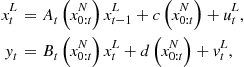
and again the form of the algorithm is unchanged; see [9] for a good coverage of the most general form of Kalman filters required in these cases.
One other important case involves nonlinear observations that are not a function of the linear state. Then the linear observation Eq. (4.62) can be generalized to ![]() , which is a general observation density. This form is quite useful in tracking examples, where observation functions are often nonlinear (range and bearings, for example, or range-only), but dynamics can be considered as linear to a good approximation [64,66,67]. If in addition the nonlinear state can be expressed in linear Gaussian state-space form with respect to the linear state, i.e.:
, which is a general observation density. This form is quite useful in tracking examples, where observation functions are often nonlinear (range and bearings, for example, or range-only), but dynamics can be considered as linear to a good approximation [64,66,67]. If in addition the nonlinear state can be expressed in linear Gaussian state-space form with respect to the linear state, i.e.:
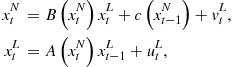
then once again the Kalman filter can be run to marginalize the linear state variable. In this case the weight expression becomes:

where now the term ![]() is computed using the Kalman filter. In some cases the linear state transition matrices and observation matrices
is computed using the Kalman filter. In some cases the linear state transition matrices and observation matrices ![]() and
and ![]() for this Kalman filter are independent of the nonlinear state and the observations; then this form of marginalized particle filter may be computed very efficiently, since the covariance matrices are identical for all particles and thus need only be computed once at each time step.
for this Kalman filter are independent of the nonlinear state and the observations; then this form of marginalized particle filter may be computed very efficiently, since the covariance matrices are identical for all particles and thus need only be computed once at each time step.
3.04.4.4.2 Further material
In this section on particle filtering we have given a general introduction. For further material please see [50,71,72]. For smoothing with particle filters, see for example [35,58,59,73–81], for parameter estimation with particle filters [34,37,63,77,82–93], and for recent combinations with MCMC [94].
3.04.5 Conclusion
This article has introduced the basic principles of parameter inference and state estimation within the Bayesian framework. We have considered a linear Gaussian parametric model by way of illustration. We have also given an introductory coverage to some of the principal computational tools available for the practitioner, including MCMC and the particle filter.
A Probability densities and integrals
A.1 Univariate Gaussian
The univariate Gaussian, or normal, density function with mean ![]() and variance
and variance ![]() is defined for a real-valued random variable as:
is defined for a real-valued random variable as:
![]() (4.70)
(4.70)
Univariate normal density.
A.2 Multivariate Gaussian
The multivariate Gaussian probability density function (PDF) for a column vector ![]() with N real-valued components is expressed in terms of the mean vector
with N real-valued components is expressed in terms of the mean vector ![]() and the covariance matrix
and the covariance matrix ![]() as:
as:
![]() (4.71)
(4.71)
Multivariate Gaussian density.
An integral which is used on many occasions throughout the text is of the general form:
![]() (4.72)
(4.72)
where ![]() is interpreted as the infinitesimal volume element:
is interpreted as the infinitesimal volume element:

and the integral is over the real line in all dimensions, i.e., the single integration sign should be interpreted as:
![]()
For non-singular symmetric ![]() it is possible to form a “perfect square” for the exponent and hence simplify the integral. Take negative of twice the exponent:
it is possible to form a “perfect square” for the exponent and hence simplify the integral. Take negative of twice the exponent:
![]() (4.73)
(4.73)
and try to express it in the form:
![]()
for some constants k and ![]() , to be determined. Multiplying out this expression leads to the required form:
, to be determined. Multiplying out this expression leads to the required form:
![]()
Here we have used the fact that ![]() , since
, since ![]() is assumed symmetric.
is assumed symmetric.
Hence, equating the constant, linear and quadratic terms in ![]() , we arrive at the result:
, we arrive at the result:
![]() (4.74)
(4.74)
where
![]()
and
Thus the integral I can be re-expressed as:
 (4.75)
where, again
![]()
Comparison with the multivariate PDF of (4.71) which has unity volume leads directly to the result:
 (4.76)
Multivariate Gaussian integral.
This result can be also be obtained directly by a transformation which diagonalizes ![]() and this approach then verifies the normalization constant given for the PDF of (4.71).
and this approach then verifies the normalization constant given for the PDF of (4.71).
A.3 Gamma density
Another distribution which will be of use is the two parameter gamma density ![]() , defined for
, defined for ![]() as
as
![]() (4.77)
(4.77)
Gamma density.
![]() is the Gamma function (see e.g., [95]), defined for positive arguments. This distribution with its associated normalization enables us to perform marginalisation of scale parameters with Gaussian likelihoods and a wide range of parameter priors (including uniform, Jeffreys, Gamma, and Inverse Gamma (see [96]) priors) which all require the following result:
is the Gamma function (see e.g., [95]), defined for positive arguments. This distribution with its associated normalization enables us to perform marginalisation of scale parameters with Gaussian likelihoods and a wide range of parameter priors (including uniform, Jeffreys, Gamma, and Inverse Gamma (see [96]) priors) which all require the following result:
![]() (4.78)
(4.78)
Gamma integral.
Furthermore the mean, mode and variance of such a distribution are obtained as:
![]() (4.79)
(4.79)
![]() (4.80)
(4.80)
![]() (4.81)
(4.81)
A.4 Inverted-gamma distribution
A closely related distribution is the inverted-gamma distribution, ![]() which describes the distribution of the variable
which describes the distribution of the variable ![]() , where Y is distributed as
, where Y is distributed as ![]() :
:
![]() (4.82)
(4.82)
Inverted-gamma density.
The IG distribution has a unique maximum at ![]() , mean value
, mean value ![]() (for
(for ![]() ) and variance
) and variance ![]() (for
(for ![]() ).
).
It is straightforward to see that the improper Jeffreys prior ![]() is obtained in the limit as
is obtained in the limit as ![]() and
and ![]() .
.
The family of IG distributions is plotted in Figure A.1 as ![]() varies over the range 0.01–1000 and with maximum value fixed at unity. The variety of distributions available indicates that it is possible to incorporate either very vague or more specific prior information about variances by choice of the mode and degrees of freedom of the distribution. With high values of
varies over the range 0.01–1000 and with maximum value fixed at unity. The variety of distributions available indicates that it is possible to incorporate either very vague or more specific prior information about variances by choice of the mode and degrees of freedom of the distribution. With high values of ![]() the prior is very tightly clustered around its mean value, indicating a high degree of prior belief in a small range of values, while for smaller
the prior is very tightly clustered around its mean value, indicating a high degree of prior belief in a small range of values, while for smaller ![]() the prior can be made very diffuse, tending in the limit to the uninformative Jeffreys prior. Values of
the prior can be made very diffuse, tending in the limit to the uninformative Jeffreys prior. Values of ![]() and
and ![]() might be chosen on the basis of mean and variance information about the unknown parameter or from estimated percentile positions on the axis.
might be chosen on the basis of mean and variance information about the unknown parameter or from estimated percentile positions on the axis.
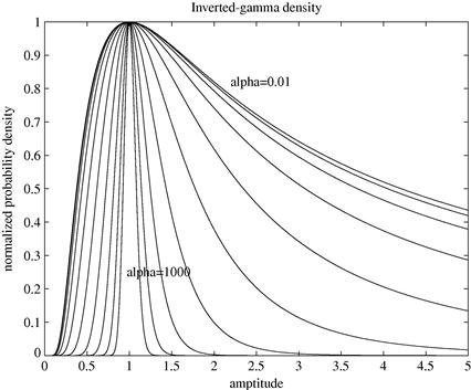
A.6 Wishart distribution
If ![]() is a
is a ![]() symmetric positive definite matrix, the Wishart distribution is defined as
symmetric positive definite matrix, the Wishart distribution is defined as
 (4.84)
where ![]() . The mean of the distribution is
. The mean of the distribution is
![]()
and the mode (maximum) is
![]()
A.7 Inverse Wishart distribution
The inverse Wishart distribution is the distribution of ![]() , where
, where ![]() has the Wishart distribution as described above,
has the Wishart distribution as described above,
 (4.85)
The mean of the distribution is
![]()
and the mode (maximum) is
![]()
References
1. Makhoul J. Linear prediction: a tutorial review. Proc IEEE. 1975;63(4):561–580.
2. Therrien CW. Discrete Random Signals and Statistical Signal Processing. Prentice-Hall 1992.
3. Bernardo JM, Smith AFM. Bayesian Theory. John Wiley & Sons 1994.
4. Box GEP, Tiao GC. Bayesian Inference in Statistical Analysis. Addison-Wesley 1973.
5. Jeffreys H. Theory of Probability. Oxford University Press 1939.
6. Robert CP. The Bayesian Choice. second ed. New York: Springer; 2001.
7. Duda RO, Hart PE. Pattern Classification and Scene Analysis. John Wiley and Sons 1973.
8. VanTrees H. Decision, Estimation and Modulation Theory, Part 1. Wiley and Sons 1968.
9. Harvey AC. Forecasting Structural Time Series Models and the Kalman Filter. Cambridge University Press 1989.
10. Kitagawa G, Gersch W. Smoothness Priors Analysis of Time Series. In: New York: Springer-Verlag; 1996; Lecture Notes in Statistics. vol. 116.
11. Zellner A. On assessing prior distributions and Bayesian regression analysis with g-prior distribution. In: Bayesian Inference and Decision Techniques: Essays in Honour of Bruno de Finetti. Elsevier 1986;233–243.
12. Akaike H. A new look at the statistical model identification. IEEE Trans Automat Control. 1974;19(6):716–723.
13. Madigan D, York J. Bayesian graphical models for discrete data. Int Stat Rev. 1995;63:215–232.
14. Dempster AP, Laird NM, Rubin DB. Maximum likelihood from incomplete data via the EM algorithm. J Roy Stat Soc Ser B. 1977;39(1):1–38.
15. Feder M, Oppenheim AV, Weinstein E. Maximum likelihood noise cancellation using the EM algorithm. IEEE Trans Acoust Speech Signal Process. 1989;37.
16. Moon TK. The expectation-maximization algorithm. IEEE Signal Process Mag. 1996;47–60.
17. Ó Ruanaidh JJK, Fitzgerald WJ. Numerical Bayesian Methods Applied to Signal Processing. Springer-Verlag 1996.
18. Weinstein E, Oppenheim AV, Feder M, Buck JR. Iterative and sequential algorithms for multisensor signal enhancement. IEEE Trans Signal Process. 1994;42.
19. Tanner MA. Tools for Statistical Inference. second ed. Springer-Verlag 1993.
20. Bishop CM. Pattern Recognition and Machine Learning. Springer 2006.
21. MacKay David JC. Information Theory, Inference, and Learning Algorithms. CUP 2003.
22. Hastings WK. Monte Carlo sampling methods using Markov chains and their applications. Biometrika. 1970;57:97–109.
23. Metropolis N, Rosenbluth AW, Rosenbluth MN, Teller AH, Teller E. Equations of state calculations by fast computing machines. J Chem Phys. 1953;21:1087–1091.
24. Tierney L. Markov chains for exploring posterior disiributions (with discussion). Ann Stat. 1994;22:1701–1762.
25. Gelfand AE, Smith AFM. Sampling-based approaches to calculating marginal densities. J Am Stat Assoc. 1990;85:398–409.
26. Geman S, Geman D. Stochastic relaxation, Gibbs distributions and the Bayesian restoration of images. IEEE Trans Pattern Anal Mach Intell. 1984;6:721–741.
27. Liu J, Wong WH, Kong A. Covariance structure of the Gibbs sampler with applications to the comparison of estimators and augmentation schemes. Biometrika. 1994;81:27–40.
28. Roberts GO, Sahu SK. Updating schemes, correlation structure, blocking and parameterization for the Gibbs sampler. J Roy Stat Soc Ser B. 1997;59:291–317.
29. Cowles MK, Carlin BP. Markov chain Monte Carlo convergence diagnostics—a comparative review. J Am Stat Assoc. 1996;91(434):883–904.
30. Godsill SJ. On the relationship between MCMC methods for model uncertainty. J Comput Graph Stat. 2001;10:230–248.
31. Green PJ. Reversible jump Markov chain Monte Carlo computation and Bayesian model determination. Biometrika. 1995;82:711–732.
32. Anderson BDO, Moore JB. Optimal Filtering. Prentice-Hall 1979.
33. Kalman RE. A new approach to linear filtering and prediction problems. ASME J Basic Eng. 1960;82:35–45.
34. Gordon N, Salmond D, Smith AF. Novel approach to nonlinear/non-Gaussian Bayesian state estimation. IEE Proc F, Radar Signal Process. 1993;140:107–113.
35. Kitagawa G. Monte-Carlo filter and smoother for non-Gaussian nonlinear state space models. J Comput Graph Stat. 1996;1:1–25.
36. West M. Mixture models, Monte Carlo, Bayesian updating and dynamic models. Comput Sci Stat. 1993;24:325–333.
37. Cappé O, Moulines E, Rydén T. Inference in Hidden Markov Models. Springer 2005.
38. Kailath T, Sayed A, Hassibi B. Linear Estimation. Prentice-Hall 2000.
39. Ristic B, Arulampalam M, Gordon A. Beyond Kalman Filters: Particle Filters for Target Tracking. Artech House 2004.
40. Jazwinski AH. Stochastic Processes and Filtering Theory. New York: Academic Press; 1970.
41. Alspach DL, Sorenson HW. Nonlinear Bayesian estimation using Gaussian sum approximation. IEEE Trans Automat Control. 1972;17(4):439–448.
42. Ito K, Xiong K. Gaussian filters for nonlinear filtering problems. IEEE Trans Automat Control. 2000;45:910–927.
43. Julier SJ, Uhlmann JK. A new extension of the Kalman filter to nonlinear systems. In: Aerosense: The 11th International Symposium on Aerospace/Defense Sensing, Simulation and Controls. 1997.
44. Van der Merwe R, Doucet A, De Freitas N, Wan E. The unscented particle filter. In: MIT Press 2000;Leen TK, Dietterich TG, Tresp V, eds. Advanced in Neural Information Processing System. vol. 13.
45. Handschin J, Mayne D. Monte Carlo techniques to estimate the conditionnal expectation in multi-stage non-linear filtering. Int J Control. 1969;9:547–559.
46. Handschin J. Monte Carlo techniques for prediction and filtering of non-linear stochastic processes. Automatica. 1970;6:555–563.
47. Blake A, Isard M. Active Contours. Springer 1998.
48. Liu J, Chen R. Blind deconvolution via sequential imputations. J Roy Stat Soc Ser B. 1995;430:567–576.
49. Del Moral P. Nonlinear filtering: interacting particle solution. Markov Process Rel Fields. 1996;2:555–579.
50. Doucet A, De Freitas N, Gordon N, eds. Sequential Monte Carlo Methods in Practice. New York: Springer; 2001.
51. Liu JS. Monte Carlo Strategies in Scientific Computing. New York: Springer; 2001.
52. Ho YC, Lee RCK. A Bayesian approach to problems in stochastic estimation and control. IEEE Trans Automat Control. 1964;9(4):333–339.
53. Pitt MK, Shephard N. Filtering via simulation: auxiliary particle filters. J Am Stat Assoc. 1999;94(446):590–599.
54. Chopin N. Central limit theorem for sequential Monte Carlo methods and its application to Bayesian inference. Ann Stat. 2004;32(6):2385–2411.
55. Crisan D, Doucet A. A survey of convergence results on particle filtering methods for practitioners. IEEE Trans Signal Process. 2002;50(3):736–746.
56. Del Moral P. Measure-valued processes and interacting particle systems, application to nonlinear filtering problems. Ann Appl Prob. 1998;8:69–95.
57. Del Moral P, Formulae Feynman-Kac. Genealogical and Interacting Particle Systems with Applications. Springer 2004.
58. Künsch HR. Recursive Monte-Carlo filters: algorithms and theoretical analysis. Ann Stat. 2005;33(5):1983–2021.
59. Doucet A, Godsill S, Andrieu C. On sequential Monte-Carlo sampling methods for Bayesian filtering. Stat Comput. 2000;10:197–208.
60. Zhang JL, Liu JS. A new sequential importance sampling method and its application to the two-dimensional hydrophobic-hydrophilic model. J Chem Phys. 2002;117.
61. Godsill S, Clapp T. Improvement strategies for Monte Carlo particle filters. In: Doucet A, De Freitas N, Gordon N, eds. Sequential Monte Carlo Methods in Practice. Springer 2001.
62. Arulampalam M, Maskell S, Gordon N, Clapp T. A tutorial on particle filters for on line non-linear/non-Gaussian Bayesian tracking. IEEE Trans Signal Process. 2002;50:241–254.
63. Shephard N, Pitt M. Likelihood analysis of non-Gaussian measurement time series. Biometrika. 1997;84(3):653–667 (Erratum in volume 91, 249–250, 2004).
64. Andrieu C, Doucet A. Particle filtering for partially observed Gaussian state space models. J Roy Stat Soc Ser B. 2002;64(4):827–836.
65. Chen R, Liu JS. Mixture Kalman filter. J Roy Stat Soc Ser B. 2000;62(3):493–508.
66. Schön T, Gustafsson F, Nordlund P-J. Marginalized particle filters for mixed linear/nonlinear state-space models. IEEE Trans Signal Process. 2005;53(7):2279–2289.
67. Karlsson R, Schön T, Gustafsson F. Complexity analysis of the marginalized particle filter. IEEE Trans Signal Process. 2005;53(11):4408–4411.
68. Kalman RE, Bucy R. New results in linear filtering and prediction theory. J Basic Eng Trans ASME, Ser D. 1961;83(3):95–108.
69. Robert CP, Casella G. Monte Carlo Statistical Methods. second ed. New York: Springer; 2004.
70. Rabiner LR. A tutorial on hidden Markov models and selected applications in speech recognition. Proc IEEE. 1989;77(2):257–285.
71. Cappé O, Godsill SJ, Moulines E. An overview of existing methods and recent advances in sequential Monte Carlo. Proc IEEE. 2007;95.
72. Doucet A, Johansen AM. A tutorial on particle filtering and smoothing: fifteen years later. In: Crisan D, Rozovsky B, eds. Oxford Handbook of Nonlinear Filtering. OUP 2011.
73. M. Briers, A. Doucet, S. Maskell, Smoothing algorithms for state-space models, Technical Report TR-CUED-F-INFENG 498, Department of Engineering, University of Cambridge, 2004.
74. Fong W, Godsill S, Doucet A, West M. Monte Carlo smoothing with application to audio signal enhancement. IEEE Trans Signal Process. 2002;50(2):438–449.
75. Godsill SJ, Doucet A, West M. Maximum a posteriori sequence estimation using Monte Carlo particle filters. Ann Inst Stat Math. 2001;53(1):82–96.
76. Godsill SJ, Doucet A, West M. Monte Carlo smoothing for non-linear time series. J Am Stat Assoc. 2004;50:438–449.
77. Hürzeler M, Künsch HR. Monte Carlo approximations for general state-space models. J Comput Graph Stat. 1998;7:175–193.
78. Isard M, Blake A. CONDENSATION—conditional density propagation for visual tracking. Int J Comput Vis. 1998;29(1):5–28.
79. Klaas M, Briers M, De Freitas N, Doucet A, Maskell S, Lang D. Fast particle smoothing: if I had a million particles. In: 23rd International Conference on Machine Learning (ICML), Pittsburgh, Pennsylvania, June 25–29. 2006.
80. Künsch HR. State space and hidden Markov models. In: Barndorff-Nielsen OE, Cox DR, Klueppelberg C, eds. Complex Stochastic Systems. Boca Raton: CRC Publisher; 2001;109–173.
81. Sarkka S, Bunch P, Godsill S. A backward-simulation based rao-blackwellized particle smoother for conditionally linear gaussian models. In: 16th IFAC Symposium on System Identification. 2012.
82. Shumway R, Stoffer D. An approach to time series smoothing and forecasting using the EM algorithm. J Time Ser Anal. 1982;3(4):253–264.
83. Andrieu C, Doucet A, Singh SS, Tadic VB. Particle methods for change detection, system identification, and control. IEEE Proc. 2004;92(3):423–438.
84. Campillo F, Le Gland F. MLE for patially observed diffusions: direct maximization vs the EM algorithm. Stochast Process Appl. 1989;33:245–274.
85. Chopin N. A sequential particle filter method for static models. Biometrika. 2002;89:539–552.
86. Del Moral P, Doucet A, Jasra A. Sequential monte carlo samplers. J Roy Stat Soc Ser B. 2006;68(3):411.
87. Fearnhead P. Markov chain Monte Carlo, sufficient statistics and particle filter. J Comput Graph Stat. 2002;11(4):848–862.
88. Gilks Walter R, Berzuini Carlo. Following a moving target—Monte Carlo inference for dynamic Bayesian models. J Roy Stat Soc Ser B. 2001;63(1):127–146.
89. Kitagawa G. A self-organizing state-space model. J Am Stat Assoc. 1998;93(443):1203–1215.
90. Liu J, West M. Combined parameter and state estimation in simulation-based filtering. In: De Freitas N, Doucet A, Gordon N, eds. Sequential Monte Carlo Methods in Practice. Springer 2001.
91. Neal RM. Annealed importance sampling. Stat Comput. 2001;11(2):125–139.
92. Jimmy Olsson, Tobias Rydén, Asymptotic properties of the bootstrap particle filter maximum likelihood estimator for state space models, Technical Report LUTFMS-5052-2005, Lund University, 2005.
93. Segal M, Weinstein E. A new method for evaluating the log-likelihood gradient, the Hessian, and the Fisher information matrix for linear dynamic systems. IEEE Trans Inform Theory. 1989;35:682–687.
94. Andrieu C, Doucet A, Holenstein R. Particle Markov chain monte carlo methods. J Roy Stat Soc Ser B (Stat Methodol.). 2010;72(3):269–342.
95. Bajpai AC, Mustoe LR, Walker D. Advanced Engineering Mathematics. Wiley 1977.
96. Manouchehr Kheradmandnia, Aspects of Bayesian Threshold Autoregressive Modelling, PhD Thesis, University of Kent, 1991.
1Whenever the context makes it unambiguous we will adopt from now on a notation ![]() to denote both probability density functions (PDFs) and probability mass functions (PMFs) for random variables and vectors.
to denote both probability density functions (PDFs) and probability mass functions (PMFs) for random variables and vectors.
2Although in time series likelihood-based analysis it is common to treat missing and other unobserved data in a Bayesian fashion, see [9,10] and references therein.
3Karlsson et al. [67] and Schön et al. [66] present a more general class of models to which the marginalized filter may be applied, but we present a more basic framework for the sake of simplicity here.