
Array Processing in the Face of Nonidealities
Mário Costa*, Visa Koivunen* and Mats Viberg†, *Department of Signal Processing and Acoustics, School of Electrical Engineering, Aalto University/SMARAD CoE, Finland, †Division of Signal Processing and Antennas, Chalmers University of Technology, Sweden
Abstract
Real-world sensor arrays are typically composed of elements with individual directional beampatterns and are subject to mutual coupling, cross-polarization effects as well as mounting platform reflections. Errors in the array elements’ positions are also common in sensor arrays built in practice. Such nonidealities need to be taken into account for optimal array signal processing and in finding related performance bounds. Moreover, problems related to beam-steering and cancellation of the signal-of-interest in beamforming applications may be prevented. Otherwise, an array processor may experience a significant performance degradation. In this chapter we provide techniques that allow the practitioner to acquire the steering vector model of real-world sensor arrays so that various nonidealities are taken into account. Consequently, array processing algorithms may avoid performance losses caused by array modeling errors. These techniques include model-based calibration and auto-calibration methods, array interpolation, as well as the wavefield modeling principle or manifold separation technique. Robust methods are also briefly considered since they are useful when the array nonidealities are not described by the employed steering vector model. Extensive array processing examples related to direction-finding and beamforming are included demonstrating that optimal or close-to optimal performance may be achieved despite the array nonidealities.
Keywords
Sensor array; Array calibration; Array processor; Array nonidealities; Wavefield modeling; Manifold separation; Beamspace transform; Array interpolation; Beamforming; Direction finding
3.19.1 Introduction
In array signal processing one is typically interested in characterizing, synthesizing, enhancing or attenuating certain aspects of propagating wavefields by employing a collection of sensors, known as a sensor array. Characterizing a propagating wavefield refers to determining its spatial spectrum, i.e., the angular distribution of energy, so that information regarding the location of the sources generating the wavefield can be obtained, for example [1]. Synthesizing or producing a wavefield refers to generating a propagating wavefield with a desired spatial spectrum in order to focus the transmitted energy towards certain locations in space. Finally, attenuating or enhancing a received wavefield based on its spatial spectrum refers to the ability of canceling interfering sources or improving the signal-to-interference-plus-noise ratio (SINR) and maximizing the energy received from certain directions. Examples of characterization, synthesis and enhancement of propagating wavefields include direction-of-arrival (DoA) estimation, angle spread estimation in channel sounding as well as transmit and receive beamforming [2].
Traditionally, array signal processing has found applications in radar and sonar, defense systems, signal intelligence (SIGINT), and surveillance as well as imaging and biomedical applications. Radioastronomy also employs many array processing techniques [3]. More recently, it has been used in wireless communication systems, in particular in basestations that utilize beamforming techniques in controlling the interference and enhancing the signal quality. Moreover, creating advanced, measurement-based models of the radio channels in communication systems such as long-term evolution (LTE) requires capturing the directional properties of the propagation channel [4]. In global navigation satellite systems, receive beamforming techniques for anti-jamming purposes are often employed as well as DoA estimation techniques in indoor navigation systems [5]. See also Chapter 20 “Applications of Array Signal Processing” in this volume.
The propagating wavefield is typically parameterized by the angular location of sources generating such a wavefield, their polarization state, bandwidth, delay profile, and Doppler shift. These are called wavefield parameters and are given in terms of a reference system, which in the case of angular information is typically assumed to be the coordinate system common to the sensor array and propagating wavefield. Such a reference system is typically assumed to be within the physical extent of the sensor array, known as array aperture, and the angular parameterization of the propagating wavefield refers to the DoAs or directions-of-departure (DoDs), characterizing the spatial spectrum of the wavefield received or transmitted by the sensor array.
In addition to the propagating wavefield, a model describing the response of the sensor array as a function of the wavefield parameters, such as the angle-of-arrival or departure, is typically required in array processing. Such a model is defined in terms of array steering vectors and allows us to estimate the wavefield parameters from data acquired by the sensor array, and use them to design a beamformer at the receiver. Similarly, steering vectors are used to synthesize a desired wavefield and employ transmit beamforming techniques. In order to simplify these signal processing tasks and models, the standard approach to array signal processing assumes rather idealistic array steering vector models. In particular, all array elements are typically assumed to have similar omnidirectional gain patterns and the employed sensor array is assumed to have a regular geometry such as a uniform linear array (ULA), a uniform rectangular array (URA), or a uniform circular array (UCA). The resulting array steering vector models have then a very convenient form for various signal processing tasks; see Section 3.19.2. However, most of real-world sensor arrays are not well described using such an ideal array model. In fact, elements of real-world arrays have individual beampatterns, not necessarily omnidirectional, and may be subject to severe mutual coupling. Phase centers of the elements may not be exactly in the assumed positions. Moreover, mounting platform reflections and cross-polarization effects are also very common in real-world arrays.
In practical array processing applications employing ideal array steering vector models leads to a performance degradation and typically to loss of optimality for optimal array processors [6]. The limiting factor in the performance of high-resolution array processing algorithms as well as in the tightness of related theoretical performance bounds is known to be the accuracy of the employed array model rather than measurement noise [6,7]. Similarly, misspecified sensor array models may lead to a severe performance loss of beamforming techniques. Effects include steering energy towards unwanted directions, cancelation of the signal of interest (SOI) as well as amplification of interfering sources [8].
In this chapter we present techniques that allow the practitioner to acquire a realistic array steering vector model by taking into account array nonidealities such as mutual coupling, mounting platform reflections, cross-polarization effects, errors in element positions as well as individual directional beampatterns. This facilitates achieving optimal performance in the presence of nonidealities as well as mitigating problems related to beam-steering, SOI and interference cancellation. We also describe how the various approaches can be applied in the context of high-resolution direction finding and beamforming. Emphasis is given to the case when the array response, along with its nonidealities, is obtained from array calibration measurements. However, the methods and techniques discussed in this chapter are also applicable when the array response is obtained from EM simulation software, or even when ideal array models are employed. Typically, EM simulation software does not capture manufacturing errors while calibration measurement noise is unavoidable in array calibration measurements. Techniques for denoising array calibration measurements are included in this chapter as well. Sensor failure in array signal processing is not addressed herein, and the interested reader is referred to [9,10] and references therein. Many of such techniques aim at determining the inoperable sensors’ outputs from the available array snapshots, and proceed with the array processing tasks as if the sensor array were fully operable. Then, realistic array steering vector models are still required and the methods discussed herein may also be useful in such circumstances.
The classification used in this chapter for the various techniques capable of dealing with array nonidealities is given in Figure 19.1. We classify the methods trying to capture the nonidealities as model-driven and data-driven techniques. Robust methods are a third class of methods that acknowledge that the array model contains errors without trying to characterize such nonidealities. Instead, robust estimation methods trade-off desirable properties such as high-resolution or optimality for reliability in the face of uncertainties in the array response. In model-driven techniques, the array nonidealities are described using an explicit formulation for each nonideality. The parameters of such a formulation may be estimated from array calibration measurements or simultaneously with wavefield parameters. The latter approach is called auto-calibration technique [7,11–14]. Data-driven techniques use array calibration data as a starting point and capture the nonidealities implicitly by using basis function expansion, interpolation, approximation or nonparametric estimation techniques. Data-driven methods include local interpolation of array calibration data [6], array interpolation technique [15–17], and manifold separation technique [18,19] which stems from the wavefield modeling principle [20–22]. These techniques do not employ any explicit model for the array nonidealities. In data-driven techniques the array nonidealities are described by the basis function coefficients, which may be estimated from array calibration measurements. Hence, they allow the practitioner to develop array processing algorithms that do not require explicit formulation for the nonidealities, are independent of the sensor array, including its geometry and individual element beampatterns while obtaining close to optimal performance. Finally, robust methods try to bound the influence of modeling errors in the estimation process instead of trying to capture them.
This chapter is organized as follows. First, conventional array steering vector models and widely employed techniques in array processing are briefly described in Section 3.19.2. Then, typical explicit formulations for array nonidealities are described in Section 3.19.3. In Section 3.19.4, array calibration measurements in controlled environments are briefly described. Section 3.19.5 includes model-driven techniques that are based on explicit formulations of the array nonidealities. Section 3.19.6 considers data-driven techniques. In Section 3.19.7, robust methods are described. Section 3.19.8 includes extensive array processing examples. Conclusions are given in Section 3.19.9.
3.19.2 Ideal array signal models
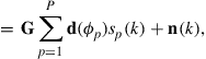
The conventional narrowband N-element array output model due to a propagating wavefield, generated by ![]() far-field sources, is
far-field sources, is
![]() (19.1)
(19.1)
where![]() , and
, and ![]() denote the array steering matrix, transmitted waveforms, and sensor noise, respectively. The discrete time instant is denoted by
denote the array steering matrix, transmitted waveforms, and sensor noise, respectively. The discrete time instant is denoted by ![]() while
while ![]() and
and ![]() represent the co-elevation and azimuth angles of the P sources generating the propagating wavefield, respectively. Typically, the co-elevation angle
represent the co-elevation and azimuth angles of the P sources generating the propagating wavefield, respectively. Typically, the co-elevation angle ![]() is measured down from the z-axis and the azimuth angle
is measured down from the z-axis and the azimuth angle ![]() is measured counter-clockwise in the xy-plane. In Eq. (19.1), the N-dimensional observation vector
is measured counter-clockwise in the xy-plane. In Eq. (19.1), the N-dimensional observation vector ![]() is known as array snapshot. The array steering matrix
is known as array snapshot. The array steering matrix ![]() is composed of P array steering vectors
is composed of P array steering vectors ![]() , each representing the array response to a plane-wave impinging on the sensor array from directions
, each representing the array response to a plane-wave impinging on the sensor array from directions ![]() . In array processing, the employed sensor array is typically assumed to be unambiguous in the sense that any collection of
. In array processing, the employed sensor array is typically assumed to be unambiguous in the sense that any collection of ![]() steering vectors with different angles forms a linearly independent set.
steering vectors with different angles forms a linearly independent set.
Assuming that the employed sensor array lies in the xy-plane, and is not subject to nonidealities such as mutual coupling or cross-polarization effects, the corresponding array steering vector model may be written as
![]() (19.2)
(19.2)
where ![]() denotes the gain function of the nth element. In (19.2),
denotes the gain function of the nth element. In (19.2), ![]() and
and ![]() denote the angular wavenumber and wavelength, respectively. Moreover,
denote the angular wavenumber and wavelength, respectively. Moreover, ![]() denote the location (in meters) of the nth element in the xy-plane, relative to the origin of the assumed coordinate system. Note that other wavefield parameters such as the polarization of the sources may also be included in the array steering vector model in (19.2). This is briefly discussed in Section 3.19.8.
denote the location (in meters) of the nth element in the xy-plane, relative to the origin of the assumed coordinate system. Note that other wavefield parameters such as the polarization of the sources may also be included in the array steering vector model in (19.2). This is briefly discussed in Section 3.19.8.
Typically, in array signal processing the steering vector model in (19.2) is further simplified by assuming that the array elements are all identical and have omnidirectional gain functions, i.e., ![]() , and are arranged in regular geometries. Commonly used ideal steering vector models include those of ULAs, UCAs, and URAs:
, and are arranged in regular geometries. Commonly used ideal steering vector models include those of ULAs, UCAs, and URAs:
![]() (19.3a)
(19.3a)
![]() (19.3b)
(19.3b)
![]() (19.3c)
(19.3c)
where ![]() and d denote the Kronecker product and the inter-element spacing, respectively. In (19.3b),
and d denote the Kronecker product and the inter-element spacing, respectively. In (19.3b), ![]() and
and ![]() denote the radius of the circular array and the angular position of the nth element, respectively.
denote the radius of the circular array and the angular position of the nth element, respectively.
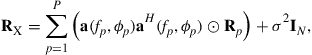
Assuming wavefield propagation in the xy-plane as well as uncorrelation between transmitted signals and sensor noise, the array covariance matrix of (19.1) is given by
![]() (19.4)
(19.4)
where ![]() and
and ![]() denote the covariance matrices of the transmitted signals and sensor noise, respectively. The signal covariance matrix
denote the covariance matrices of the transmitted signals and sensor noise, respectively. The signal covariance matrix ![]() may be rank deficient, with rank
may be rank deficient, with rank ![]() , due to highly correlated or coherent sources that may be caused by specular multipath propagation, for example. Sensor noise is typically assumed to be zero-mean complex-circular Gaussian distributed
, due to highly correlated or coherent sources that may be caused by specular multipath propagation, for example. Sensor noise is typically assumed to be zero-mean complex-circular Gaussian distributed ![]() . In practice, the exact covariance matrix in (19.4) is unknown and it is typically estimated from a collection of
. In practice, the exact covariance matrix in (19.4) is unknown and it is typically estimated from a collection of ![]() array snapshots as
array snapshots as
 (19.5)
Signal models (19.1) and (19.4) are used in most array processing tasks such as beamforming and direction finding. In estimation problems, maximum likelihood methods are commonly used to find the optimal parameter estimates whereas beamformers typically target at enhancing the signal by maximizing the SINR at the array output.
A popular criterion for evaluating the performance of beamformers is the array output SINR [8]:
 (19.6)
where ![]() and
and ![]() denote the angle from where the SOI impinges on the sensor array and the corresponding signal power, respectively. Moreover,
denote the angle from where the SOI impinges on the sensor array and the corresponding signal power, respectively. Moreover, ![]() denotes the beamformer weight vector and
denotes the beamformer weight vector and ![]() the covariance matrix due to both interfering signals
the covariance matrix due to both interfering signals ![]() and sensor noise. The optimal weight vector that maximizes (19.6) is [8]
and sensor noise. The optimal weight vector that maximizes (19.6) is [8]
![]() (19.7)
(19.7)
where ![]() may be arbitrary since it does not affect the SINR in (19.6). Choosing
may be arbitrary since it does not affect the SINR in (19.6). Choosing ![]() leads to the well-known minimum variance distortionless response (MVDR) beamformer, also known as Capon beamformer [8,23]. Note that using the exact
leads to the well-known minimum variance distortionless response (MVDR) beamformer, also known as Capon beamformer [8,23]. Note that using the exact ![]() in place of
in place of ![]() in (19.7) does not affect the array output SINR.
in (19.7) does not affect the array output SINR.
In Section 3.19.1, we have mentioned that the DoAs of the sources generating the propagating wavefield may be found from its spatial spectrum. The location of the sources are associated with the angles of the spatial spectrum with larger power. We may therefore view DoA estimation as a spectrum estimation problem and employ beamforming techniques for estimating the angular distribution of power of the wavefield received by the sensor array. Such an approach is called nonparametric or spectral-based approach to DoA estimation since it does not require a parametric model for the sources, nor the number of sources generating the wavefield. These techniques are versatile but typically have poor resolution and lead to suboptimal DoA estimates. Informally, resolution refers to the ability of distinguishing between two closely spaced sources. The resolution of beamforming techniques is limited by the array aperture, i.e., the physical size of the array in wavelengths, as well as SNR, and does not improve with increasing number of array snapshots.
One way of improving the resolution limit imposed by the array aperture is by making further assumptions regarding the sources generating the propagating wavefield. In particular, we first assume that the number of sources P as well as rank of the signal covariance matrix ![]() are known or have been correctly estimated from the array output. The radiating sources are also assumed to be located in the far-field of the sensor arrays as well as point-emitters in the sense that the field radiated by each source can be assumed to have originated from a single location in space. Finally, we assume that the number of sources generating the wavefield is smaller than the number of array elements. Then, the array output in (19.1) is known as low-rank signal model and the array covariance matrix in (19.4) can be written as
are known or have been correctly estimated from the array output. The radiating sources are also assumed to be located in the far-field of the sensor arrays as well as point-emitters in the sense that the field radiated by each source can be assumed to have originated from a single location in space. Finally, we assume that the number of sources generating the wavefield is smaller than the number of array elements. Then, the array output in (19.1) is known as low-rank signal model and the array covariance matrix in (19.4) can be written as
![]() (19.8)
(19.8)
Here, ![]() and
and ![]() contain the eigenvectors of
contain the eigenvectors of ![]() spanning the so-called signal and noise subspaces while
spanning the so-called signal and noise subspaces while ![]() and
and ![]() contain the corresponding eigenvalues in their diagonal. Techniques employing the low-rank signal model are called subspace methods and are a class of high-resolution DoA estimation algorithms [2]. They exploit the fact that the columns of
contain the corresponding eigenvalues in their diagonal. Techniques employing the low-rank signal model are called subspace methods and are a class of high-resolution DoA estimation algorithms [2]. They exploit the fact that the columns of ![]() span the same subspace as the columns of the steering matrix
span the same subspace as the columns of the steering matrix ![]() (in the case of coherent signals
(in the case of coherent signals ![]() is contained in the subspace spanned by the columns of
is contained in the subspace spanned by the columns of ![]() ), and that both
), and that both ![]() and
and ![]() are orthogonal to
are orthogonal to ![]() . Unlike beamforming techniques, the resolution of subspace methods improves with increasing number of array snapshots.
. Unlike beamforming techniques, the resolution of subspace methods improves with increasing number of array snapshots.
A commonly used lower bound on the estimation error variance of any unbiased estimator is the Cramér-Rao lower Bound (CRB) [24]. Assuming that both signal and noise are zero-mean complex-circular Gaussian distributed, the unconditional CRB for azimuth angle estimation is [25]
![]() (19.9)
(19.9)
where ![]() . Moreover,
. Moreover, ![]() and
and ![]() denote the Hadamard-Schur product and a projection matrix onto the nullspace of
denote the Hadamard-Schur product and a projection matrix onto the nullspace of ![]() , respectively. An estimator with an error covariance matrix that equals (19.9) is called statistically efficient. In particular, the stochastic maximum likelihood estimator is asymptotically
, respectively. An estimator with an error covariance matrix that equals (19.9) is called statistically efficient. In particular, the stochastic maximum likelihood estimator is asymptotically ![]() statistically efficient, and the azimuth-angle estimates are obtained as [26]
statistically efficient, and the azimuth-angle estimates are obtained as [26]
![]() (19.10)
(19.10)
Here, ![]() denotes the determinant of a matrix. Moreover,
denotes the determinant of a matrix. Moreover, ![]() and
and ![]() denote estimates of the signal covariance matrix and sensor noise, respectively. See [26] and chapter DOA Estimation Methods and Algorithms of this book for details.
denote estimates of the signal covariance matrix and sensor noise, respectively. See [26] and chapter DOA Estimation Methods and Algorithms of this book for details.
Asymptotically optimal DoA estimation algorithms such as the stochastic maximum likelihood estimator, and beamforming techniques such as the Capon beamformer, are often very sensitive to uncertainties in the array steering vector model and sensor noise (and interferers) statistics [6,8]. Under these scenarios, optimal DoA estimators may be subject to bias and increased variance while optimum beamformers may suffer from SOI cancellation effect. Uncertainty in noise statistics may be due to outliers, i.e., highly deviating observations that do not follow the same pattern as the majority of the data, or incorrect assumptions on the noise environment. For example, man-made interference has typically a non-Gaussian heavy-tailed distribution, for which (19.5) may no longer be a consistent estimator of ![]() [27]. Uncertainties in the steering vector model are often due to misspecification or lack of knowledge of various array nonidealities. These include:
[27]. Uncertainties in the steering vector model are often due to misspecification or lack of knowledge of various array nonidealities. These include:
• Uncertainty in array elements’ beampatterns and positions.
• Mounting platform reflections.
• Departures from narrowband, far-field and point-source assumptions.
In subsequent sections we describe in detail various rigorous and practical approaches for taking the aforementioned nonidealities of real-world arrays into account by array processing techniques. For details on array processing under uncertainty in noise statistics the reader is referred to [27].
3.19.3 Examples of array nonidealities
This section describes the main nonidealities experienced in real-world sensor arrays. We discuss their effects in array processing techniques, and provide explicit formulations describing such array nonidealities that can be found in the literature. These models are rather specific but allow one to understand the departure from the ideal array model as well as to incorporate such nonidealities into both DoA estimators and beamforming techniques.
3.19.3.1 Mutual coupling
Mutual coupling (also known as cross-talk) refers to interactions among array elements. The signal received by an element affects the signals received by the other array elements, and similarly for signal transmission [28, Chapter 2]. Typically, mutual coupling is inversely proportional to the inter-element spacing as well as isolation among array elements. Mutual coupling distorts the elements’ radiation patterns and decreases the efficiency of sensor arrays. Mobile wireless terminals equipped with antenna arrays are a typical example where mutual coupling is significant since the whole chassis, along with its other components, can be considered part of the antenna [5]. Array processing algorithms typically experience a significant loss of performance when the employed array steering vector model does not account for mutual coupling [6,29].
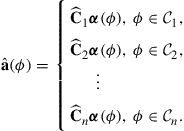
The steering vector of a sensor array subject to mutual coupling is typically modeled as [6]
![]() (19.11)
(19.11)
where ![]() denotes the mutual coupling matrix and
denotes the mutual coupling matrix and ![]() is known as nominal array steering vector. The
is known as nominal array steering vector. The ![]() element describes the contribution of the nth array element to the output of the mth sensor. Nominal sensor arrays are typically considered to be ideal uniform arrays with regular geometries of the form (16.3), and the motivation for their use is based on the assumption that real-world arrays may be described as a perturbation from an ideal sensor array. For example, if the nominal array is assumed to be an ideal UCA the mutual coupling matrix takes the form of a circulant matrix [30]. Note that a diagonal matrix
element describes the contribution of the nth array element to the output of the mth sensor. Nominal sensor arrays are typically considered to be ideal uniform arrays with regular geometries of the form (16.3), and the motivation for their use is based on the assumption that real-world arrays may be described as a perturbation from an ideal sensor array. For example, if the nominal array is assumed to be an ideal UCA the mutual coupling matrix takes the form of a circulant matrix [30]. Note that a diagonal matrix ![]() in (19.11) may also describe errors due to the receiver front-end such as imbalance in the I/Q channels. This is also discussed in Section 3.19.3.5.
in (19.11) may also describe errors due to the receiver front-end such as imbalance in the I/Q channels. This is also discussed in Section 3.19.3.5.
In practice, the mutual coupling matrix needs to be determined from array calibration measurements and a nominal array steering vector should be specified by the practitioner. Typically, the mutual coupling matrix is obtained from the measured network parameters of the sensor array, including scattering and transmission coefficients, which may be a rather tedious task [31,32, Chapter 2]. Moreover, determining the nominal array steering vector is typically based on trial and error, and rely on visual inspection of the real-world sensor array.
3.19.3.2 Uncertainty in array elements’ beampatterns and positions
Often, elements’ beampatterns and positions in real-world arrays are not fully known. This may be caused by normal variability in the manufacturing process in the sense that each array element has an individual beampattern or may suffer from manufacturing errors. In fact, elements’ phase centers in real-world arrays do not typically correspond to their physical locations due to interactions with other array elements and mounting platform. Misspecification of the array element’s beampatterns and phase centers leads to loss of performance in array processing techniques.
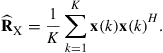
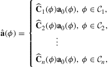
A commonly employed model taking into account individual beampatterns and position errors is
![]() (19.12)
(19.12)
where ![]() , and
, and ![]() denote the error in the nth element’s position, with respect to the nominal array steering vector, and corresponding directional beampattern. Parameters
denote the error in the nth element’s position, with respect to the nominal array steering vector, and corresponding directional beampattern. Parameters ![]() may be estimated from calibration measurements taken in controlled environments while the gain function
may be estimated from calibration measurements taken in controlled environments while the gain function ![]() may be measured at a discrete set of points and interpolated using appropriate basis functions such as splines [6]. The latter approach leads to a technique known as array interpolation and it is described in Section 3.19.6.
may be measured at a discrete set of points and interpolated using appropriate basis functions such as splines [6]. The latter approach leads to a technique known as array interpolation and it is described in Section 3.19.6.
Alternatively, one may specify a parametric model for ![]() (i.e., functionally dependent on
(i.e., functionally dependent on ![]() ) by trial and error, and visual inspection. For example, in the case of electrically short (relative to the wavelength) x-oriented dipoles one can use the following approximation
) by trial and error, and visual inspection. For example, in the case of electrically short (relative to the wavelength) x-oriented dipoles one can use the following approximation ![]() . However, in the general case of electrically large antennas and patch elements, specifying a parametric model for
. However, in the general case of electrically large antennas and patch elements, specifying a parametric model for ![]() may be very challenging. An example of two gain functions of a real-world array is illustrated in Figure 19.2b.
may be very challenging. An example of two gain functions of a real-world array is illustrated in Figure 19.2b.
3.19.3.3 Cross-polarization effects
Cross-polarization effects refer to “leakage” that, for example, a vertically polarized element suffers from an horizontally polarized wavefield. They are typically characterized by the cross-polarization discrimination (XPD), denoting the ratio between the power received by an antenna due to co-polarized and cross-polarized wavefields. The ratio between the powers received in different polarizations is commonly expressed in dB scale. XPD defines quantitatively how well the two received channels that use different polarization orientations are isolated. Antennas with a large XPD are essentially insensitive to cross-polarization effects and the power received from cross-polarized wavefields may be neglected. When mounted on an array the antennas’ XPD may change significantly due to complex EM interactions among the array elements, scatterers, and mounting platform. In such cases, high-resolution DoA estimators that do not take cross-polarization effects into account typically lead to estimates that may contain significant bias and excess variance [33].
The steering vector of a sensor array that is subject to cross-polarization effects may be described as
![]() (19.13)
(19.13)
where ![]() and
and ![]() denote the array responses due to a co-polarized and cross-polarized wavefields, respectively. Moreover,
denote the array responses due to a co-polarized and cross-polarized wavefields, respectively. Moreover, ![]() define the polarization of the wavefield. For example, for a co-polarized wavefield Eq. (19.13) simplifies to
define the polarization of the wavefield. For example, for a co-polarized wavefield Eq. (19.13) simplifies to ![]() while for a cross-polarized wavefield we have
while for a cross-polarized wavefield we have ![]() .
.
Parametric modeling of ![]() and
and ![]() in (19.13) may now be done by employing models (19.11) and (19.12). However, specifying a nominal array steering vector model for the cross-polarized component
in (19.13) may now be done by employing models (19.11) and (19.12). However, specifying a nominal array steering vector model for the cross-polarized component ![]() is even more challenging than that of the co-polarized component, where one may approximate the element’s gain function as
is even more challenging than that of the co-polarized component, where one may approximate the element’s gain function as ![]() . Typically, visual inspection does not help much in determining a parametric model for
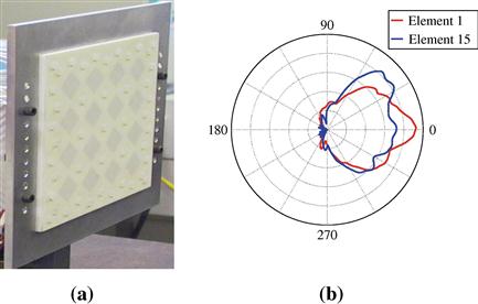
. Typically, visual inspection does not help much in determining a parametric model for ![]() . An example of gain functions corresponding to an horizontally and vertically polarized wavefield is illustrated in Figure 19.3.
. An example of gain functions corresponding to an horizontally and vertically polarized wavefield is illustrated in Figure 19.3.
Figure 19.3 Gain functions corresponding to the horizontal and vertical polarization components of an element of the real-world rectangular array from Figure 19.2a.
3.19.3.4 Departures from narrowband assumption
The narrowband signal model commonly used in array processing (see Section 3.19.2) assumes that the time-bandwidth product is “small,” i.e.,
![]() (19.14)
(19.14)
where ![]() and
and ![]() denote the bandwidth of the transmitted signal and the wavefront’s propagation delay across the array aperture, respectively. A rule of thumb for considering a signal narrowband is
denote the bandwidth of the transmitted signal and the wavefront’s propagation delay across the array aperture, respectively. A rule of thumb for considering a signal narrowband is ![]() [34]. In practice, the time-bandwidth product may be such that the narrowband assumption no longer holds true. This is also the case in focusing-based wideband array processing, where signals’ bandwidth is divided into a set of narrowband channels and narrowband processing is applied to each narrowband bin or to a focused covariance matrix [35]. Alternatively, genuine space-time signal processing can be employed as in STAP radar systems [36,37].
[34]. In practice, the time-bandwidth product may be such that the narrowband assumption no longer holds true. This is also the case in focusing-based wideband array processing, where signals’ bandwidth is divided into a set of narrowband channels and narrowband processing is applied to each narrowband bin or to a focused covariance matrix [35]. Alternatively, genuine space-time signal processing can be employed as in STAP radar systems [36,37].
Assuming an array with a flat frequency response (with linear phase) over the signals’ bandwidth, the array covariance matrix may be modeled as [34,38]
 (19.15)
where ![]() denotes the element-wise Hadamard-Schur product. Moreover,
denotes the element-wise Hadamard-Schur product. Moreover, ![]() denotes the array steering vector with a linear phase response over frequency and
denotes the array steering vector with a linear phase response over frequency and ![]() contains the correlation of the pth signal among the array elements. For signals with small time-bandwidth product
contains the correlation of the pth signal among the array elements. For signals with small time-bandwidth product ![]() equals a matrix of ones and (19.15) reduces to (19.4). However, when
equals a matrix of ones and (19.15) reduces to (19.4). However, when ![]() is non-negligible the rank of
is non-negligible the rank of ![]() due to a single signal is larger than one, and the low-rank structure of the array covariance matrix in (19.4) is lost. Thus, high-resolution subspace methods may not be applicable anymore [34]. The influence of non-negligible time-bandwidth product on DoA estimators and beamforming techniques has been addressed in [34,38]. In most cases, the error due to non-negligible time-bandwidth product can be neglected when compared to finite sample effects. However, when sources are closely spaced or have large difference in power, such an error may be significant.
due to a single signal is larger than one, and the low-rank structure of the array covariance matrix in (19.4) is lost. Thus, high-resolution subspace methods may not be applicable anymore [34]. The influence of non-negligible time-bandwidth product on DoA estimators and beamforming techniques has been addressed in [34,38]. In most cases, the error due to non-negligible time-bandwidth product can be neglected when compared to finite sample effects. However, when sources are closely spaced or have large difference in power, such an error may be significant.
3.19.3.5 Errors due to receiver front-end architectures
Receiver architectures are commonly classified as superheterodyne, low-IF (intermediate frequency) or direct-conversion receivers. Each front-end architecture is subject to various nonidealities such as I/Q-imbalance, DC-offset, and interfering image frequencies that impact the performance of array processors.
Superheterodyne receivers typically consist of two or more IF stages in order to convert the radio-frequency (RF) signal to baseband. They require image rejection filters at each downconversion stage, which may be difficult to integrate on-chip with other components. Power consumption and size may be significant [39]. Low-IF receivers convert the RF signal to baseband in two IF stages, similarly to the superheterodyne receiver. The need for image rejection filters is overcome by the use of two mixers, one for each I/Q channels, in order to cancel the image. In practice, gain and phase imbalances in the I/Q channels limit the effectiveness of such image cancellation approach. Direct-conversion (or zero-IF) receivers downconvert the RF signal to baseband in a single stage. There is no need for image rejection filters nor image cancellation. However, they typically suffer from DC offset, and I/Q imbalances in the demodulation process are still present.
I/Q imbalances in the demodulation process are common to all of the aforementioned receivers and have been studied in the context of array signal processing in [40]. They appear as phase and amplitude distortions in the I and Q branches of the demodulated signal. Similarly to errors caused by departures from narrowband assumption, the rank of the covariance matrix due to received signals increases by two and the noise eigenvalues are no longer identical. The low-rank structure of the array covariance matrix may be lost and subspace-based array processing methods experience a performance degradation.
One should note that I/Q imbalances may be significantly mitigated by using advanced digital downconverters, either at intermediate or radio frequencies. The commonly used low-rank model is then a good approximation of the array covariance matrix, given that a sufficient number of quantization bits are used [41]. Power consumption and high cost of ADCs operating at GHz and large bandwidths may be a limiting factor in practice.
We also note that antenna arrays using a single receiver, known as switched or time division multiplexing receivers, are often employed in practice due to their low-power, cost, and size [41,42]. Typically, switched array receivers suffer from phase errors that need to be estimated and taken into account by array processing methods.
3.19.3.6 Effects of nonlinear elements
Linearity of the sensor array is among the most common assumptions in the array processing literature. Linearity, in the sense of superposition principle, essentially means that the array output due to a propagating wavefield generated by multiple sources equals the sum of array outputs due to a wavefield generated by each source separately. Most sensor arrays can be considered linear systems and the superposition principle may then be employed [32]. However, active elements such as low-noise amplifiers (LNAs) commonly used in receiver architectures are nonlinear systems and the superposition principle at the array output (after the RF front-end) may no longer hold true [43]. Typically, LNAs trade-off linearity for gain and noise figures. Some waveforms that have large peak to average power ratio such as OFDM (orthogonal frequency-division multiplexing) are particularly sensitive to nonlinearities of power amplifiers. Digital signal processing techniques for mitigating nonlinear effects due to RF front-end include pre- as well as post-distortion techniques [44].
3.19.4 Array calibration
The goal of array calibration is to capture the combined effects of sensor positions, their unknown gain and phase, mutual coupling characteristics as well as cross-polarization effects and mounting platform reflections. In array calibration one typically acquires the so-called array measurement matrix ![]() . The array measurement matrix is composed of a collection of Q steering vectors corresponding to the angles contained in the vector
. The array measurement matrix is composed of a collection of Q steering vectors corresponding to the angles contained in the vector ![]() . The standard approach of obtaining the array measurement matrix is by taking the sensor array into an anechoic chamber and measuring its response to a source, known as probe, from
. The standard approach of obtaining the array measurement matrix is by taking the sensor array into an anechoic chamber and measuring its response to a source, known as probe, from ![]() different known angles. The antenna array is usually mounted on a mechanical device, called positioner, that rotates the sensor array in azimuth (and possibly in elevation) while the probe is held fixed; see Figure 19.4. Note that the coordinate system employed for DoA estimation is defined by both the positioner and probe.
different known angles. The antenna array is usually mounted on a mechanical device, called positioner, that rotates the sensor array in azimuth (and possibly in elevation) while the probe is held fixed; see Figure 19.4. Note that the coordinate system employed for DoA estimation is defined by both the positioner and probe.
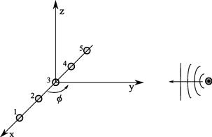
Figure 19.4 Example of the standard array calibration setup. A ULA is rotated in the xy-plane around its center element while a probe is held fixed in the far-field of the ULA.
The array measurement matrix fully describes a given real-world sensor array as well as all its nonidealities. However, array calibration measurements are typically taken in controlled environments such as anechoic chambers, and may be subject to various errors including sensor noise, reflections from the anechoic chamber, imperfections of the employed positioner, attenuations and phase-drifts due to cabling, small distance between the antenna array and probe (i.e., not in far-field), and effects of the probe (e.g., not a point-source). These errors need to be corrected so that array processing techniques may employ an accurate model of the real-world array response. Approaches for reducing the aforementioned errors occurring during array calibration measurements can be found in [32,33,45]. Moreover, array calibration measurements do not provide any steering vector model, i.e., an explicit formulation describing the array response as a function of the wavefield parameters. Such difficulties may be alleviated by employing data-driven techniques described in Section 3.19.6.
Typically, the array measurement matrix contains the array response to angles spanning the whole angular region, such as ![]() in the azimuth-only case. However, in some applications the array response may only be measured over a small angular sector, and a partial array calibration is obtained. Examples include applications where the antenna array is deployed on an environment where the sources are known a priori to be confined to an angular sector or when the array dimensions do not allow a full calibration. Data-driven techniques described in Section 3.19.6 are also applicable in these cases.
in the azimuth-only case. However, in some applications the array response may only be measured over a small angular sector, and a partial array calibration is obtained. Examples include applications where the antenna array is deployed on an environment where the sources are known a priori to be confined to an angular sector or when the array dimensions do not allow a full calibration. Data-driven techniques described in Section 3.19.6 are also applicable in these cases.
3.19.5 Model-driven techniques
In this section, we describe techniques that assume an explicit model describing each array nonideality. The array nonidealities may be estimated, by employing such a model, from array calibration measurements or directly from the array output data, simultaneously with the wavefield parameters. The latter approach is known as auto-calibration technique. Moreover, the array nonidealities may be assumed to be unknown deterministic or random parameters with known prior distribution. Hence, methods from estimation theory may be applied to estimate the array nonidealities.
3.19.5.1 Deterministic approach
Consider an N-element planar array lying in the xy-plane and denote the uncertainty in the array elements’ positions by ![]() . In this case, the array is not assumed to be subject to other nonidealities such as cross-polarization effects or individual beampatterns. We may estimate the sensors’ misplacements
. In this case, the array is not assumed to be subject to other nonidealities such as cross-polarization effects or individual beampatterns. We may estimate the sensors’ misplacements ![]() from array calibration measurements as [6]
from array calibration measurements as [6]
![]() (19.16)
(19.16)
where ![]() denotes a matrix composed of a collection of array steering vectors describing
denotes a matrix composed of a collection of array steering vectors describing ![]() in a closed-form, such as in (19.12), and
in a closed-form, such as in (19.12), and ![]() denotes the Frobenius norm of a matrix. In some cases, a closed-form solution to (19.16) may be obtained. For example, using the mutual coupling matrix
denotes the Frobenius norm of a matrix. In some cases, a closed-form solution to (19.16) may be obtained. For example, using the mutual coupling matrix ![]() in place of
in place of ![]() in (19.16) yields the following solution:
in (19.16) yields the following solution:
![]() (19.17)
(19.17)
where we have used the array model (19.11) and assumed that ![]() has full row-rank. Notation
has full row-rank. Notation ![]() in (19.17) denotes the Moore-Penrose pseudo-inverse of a matrix. Similarly, by letting
in (19.17) denotes the Moore-Penrose pseudo-inverse of a matrix. Similarly, by letting ![]() denote angle-independent gain and phase errors such as
denote angle-independent gain and phase errors such as ![]() , we obtain the following solution:
, we obtain the following solution:
![]() (19.18)
(19.18)
where ![]() and
and ![]() denote the nth row of
denote the nth row of ![]() and
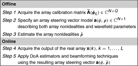
and ![]() , respectively. In case one is dealing with electrically large uniform linear arrays, the mutual coupling matrix may be approximated by a banded matrix. Recall that mutual coupling is typically inversely proportional to inter-element spacing thus, such an effect may be negligible among sensors located at both ends of the linear array. A least-squares estimator to such a structured mutual coupling matrix may also be found in a closed-form. Computationally efficient solutions may employ appropriate LU-factorization and back-substitution methods [46, Chapter 4]. A summary of model-driven calibration is given in Table 19.1.
, respectively. In case one is dealing with electrically large uniform linear arrays, the mutual coupling matrix may be approximated by a banded matrix. Recall that mutual coupling is typically inversely proportional to inter-element spacing thus, such an effect may be negligible among sensors located at both ends of the linear array. A least-squares estimator to such a structured mutual coupling matrix may also be found in a closed-form. Computationally efficient solutions may employ appropriate LU-factorization and back-substitution methods [46, Chapter 4]. A summary of model-driven calibration is given in Table 19.1.
Alternatively, we may jointly estimate array nonidealities and wavefield parameters from the output of the sensor array [11–13]. For example, joint estimation of the nonidealities ![]() and azimuth angles of P sources
and azimuth angles of P sources ![]() generating a propagating wavefield may be accomplished by employing the following nonlinear least-squares estimator [12]
generating a propagating wavefield may be accomplished by employing the following nonlinear least-squares estimator [12]
![]() (19.19)
(19.19)
Typically, criterion in (19.19) is minimized in an alternating manner between the array nonidealities ![]() and the DoAs
and the DoAs ![]() [47]. Since (19.19) is highly nonlinear, and potentially with multiple local minima, the minimization should be initialized with “good enough” initial values so that the global minimum can be attained. Note that the array nonidealities
[47]. Since (19.19) is highly nonlinear, and potentially with multiple local minima, the minimization should be initialized with “good enough” initial values so that the global minimum can be attained. Note that the array nonidealities ![]() are typically nuisance parameters. The statistical performance of the wavefield parameter estimates may suffer due to the higher dimension of the parametric model as well as estimation errors in the nuisance parameters.
are typically nuisance parameters. The statistical performance of the wavefield parameter estimates may suffer due to the higher dimension of the parametric model as well as estimation errors in the nuisance parameters.
The main issue with auto-calibration techniques is that of parameter identifiability [6]. In general, both ![]() and
and ![]() cannot be uniquely estimated unless a nonlinear sensor array is employed and additional assumptions regarding sensors’ locations as well as DoAs are made [12,13]. For example, if the array orientation is unknown the DoAs may not be uniquely estimated since they represent the angles relative to the orientation of the sensor array. Alternatively, one may assume that the array nonidealities are random parameters with a known prior distribution, and employ Bayesian estimators. This is discussed next.
cannot be uniquely estimated unless a nonlinear sensor array is employed and additional assumptions regarding sensors’ locations as well as DoAs are made [12,13]. For example, if the array orientation is unknown the DoAs may not be uniquely estimated since they represent the angles relative to the orientation of the sensor array. Alternatively, one may assume that the array nonidealities are random parameters with a known prior distribution, and employ Bayesian estimators. This is discussed next.
3.19.5.2 Bayesian approach
In the previous section we have seen that the identifiability problem in auto-calibration techniques could be alleviated by making additional assumptions regarding the nonidealities or wavefield parameters. One such an assumption considers the array nonidealities to be random parameters with a known prior distribution. In addition to alleviating the identifiability problem, such an assumption allows one (at least in principle) to “integrate out” the array nonidealities and focus on the wavefield parameters, instead [24]. For example, in mass production of sensor arrays one could model array elements’ misplacements due to manufacturing errors as bivariate Gaussian distributed and proceed with Bayesian type of estimators for the wavefield parameters [7,14].
One such an estimator is the generalized weighted subspace fitting (GWSF) algorithm proposed in [7]. It extends the MODE [48] and WSF [49] by taking into account prior information (first and second moments) of the array nonidealities in an optimal manner. It provides asymptotically efficient estimates provided the assumption on the prior Gaussian distribution is valid and array parameterization is known. The DoA estimates obtained by the GWSF are given by [7]
![]() (19.20)
(19.20)
where ![]() and
and ![]() denotes a projection matrix onto the orthogonal complement of
denotes a projection matrix onto the orthogonal complement of
 (19.21)
Furthermore, ![]() in (19.20) denotes a (positive-definite) weighting matrix that ensures asymptotically minimum variance unbiased estimates and the superscript
in (19.20) denotes a (positive-definite) weighting matrix that ensures asymptotically minimum variance unbiased estimates and the superscript ![]() denotes complex-conjugate. The first and second-order moments of the array nonidealities enter criterion (19.20) through
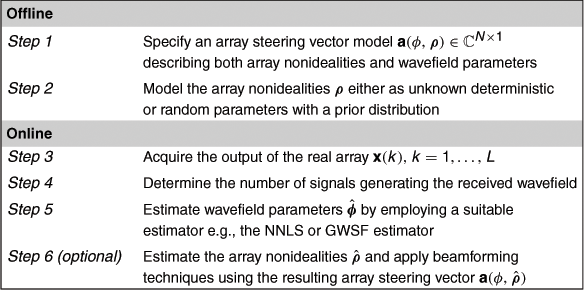
denotes complex-conjugate. The first and second-order moments of the array nonidealities enter criterion (19.20) through ![]() ; see [7] for details. Criterion (19.20) is an asymptotic approximation of the maximum a posteriori estimator for simultaneous estimation of array and wavefield parameters [14]. It may be implemented by means of polynomial rooting techniques when the nominal array steering vector has a form similar to that of an ideal ULA. A summary of auto-calibration techniques is given in Table 19.2.
; see [7] for details. Criterion (19.20) is an asymptotic approximation of the maximum a posteriori estimator for simultaneous estimation of array and wavefield parameters [14]. It may be implemented by means of polynomial rooting techniques when the nominal array steering vector has a form similar to that of an ideal ULA. A summary of auto-calibration techniques is given in Table 19.2.
The main difficulty with the Bayesian approach is related to the well-known problem of choosing appropriate prior distributions.1 Assumed prior knowledge may not exist or it may be difficult to express in the form of a pdf. Moreover, specifying a parametric model for the array nonidealities may be very challenging in practice, similarly to the deterministic approach. In case of uncertainties in the array elements’ locations, the nominal steering vector model may be obtained by visual inspection of the real-world sensor array [7]. However, when considering cross-polarization effects, sensors with individual beampatterns and mutual coupling, such a procedure is of little help in determining a nominal array steering vector.
In practice, array calibration measurements may be necessary even in auto-calibration techniques. Hence, it may be worth considering alternative techniques for dealing with array nonidealities that assume array calibration measurements but do not suffer from the difficulties in specifying explicit formulations for the nonidealities. This is discussed in the next section.
3.19.6 Data-driven techniques
Data-driven techniques take into account all array nonidealities simultaneously through array calibration measurements or synthesized array response using e.g., electromagnetic simulation software. These techniques do not require any explicit formulation describing the array nonidealities in a closed-form. Examples of nonidealities that may be handled with data-driven techniques include mutual coupling, individual beampatterns, mounting platform reflections, and cross-polarization effects. This section describes the array interpolation technique [15] and wavefield modeling principle [20], also known as manifold separation technique [18].
In particular, array interpolation technique may be understood as a linear interpolation method that fits array calibration measurements with some ideal array steering vector model. The manifold separation techniques stems from the wavefield modeling principle and can be seen as an orthogonal expansion in Fourier basis (in azimuth-angle processing) of each array element. The expansion coefficients describe the array nonidealities in a combined manner and may be estimated from array calibration measurements.
3.19.6.1 Local interpolation of the array calibration matrix
The columns of the array calibration matrix ![]() discussed in Section 3.19.4 describe the array response, with the combined effects due to array nonidealities, to a set of angles. The angular grid employed in array calibration measurements is typically sparse due to time and cost limitations. Hence, optimal array processing methods using the array calibration matrix may loose their high-resolution properties and suffer from SOI cancellation effects. Perhaps the most intuitive approach to overcome such a limitation consists in interpolating the array calibration matrix using local basis functions such as splines.
discussed in Section 3.19.4 describe the array response, with the combined effects due to array nonidealities, to a set of angles. The angular grid employed in array calibration measurements is typically sparse due to time and cost limitations. Hence, optimal array processing methods using the array calibration matrix may loose their high-resolution properties and suffer from SOI cancellation effects. Perhaps the most intuitive approach to overcome such a limitation consists in interpolating the array calibration matrix using local basis functions such as splines.
Let ![]() denote a vector composed of local basis functions such as splines or other polynomial functions. The practitioner should choose local basis functions with desirable properties such as smoothness, differentiability, and minimum energy. Also, let
denote a vector composed of local basis functions such as splines or other polynomial functions. The practitioner should choose local basis functions with desirable properties such as smoothness, differentiability, and minimum energy. Also, let ![]() denote a coefficient matrix obtained by interpolating the array calibration matrix
denote a coefficient matrix obtained by interpolating the array calibration matrix ![]() over an angular sector
over an angular sector ![]() using
using ![]() .
. ![]() may correspond to two or more columns of
may correspond to two or more columns of ![]() . Using local basis as the interpolating functions leads to the following piece-wise estimate of the real-world array steering vector:
. Using local basis as the interpolating functions leads to the following piece-wise estimate of the real-world array steering vector:
 (19.22)
Alternatively, one may use a nominal array steering vector ![]() in place of
in place of ![]() , and use a local basis expansion for the coefficients matrices in (19.22), instead. More precisely, we may have [6]:
, and use a local basis expansion for the coefficients matrices in (19.22), instead. More precisely, we may have [6]:
 (19.23)
where the nth matrix ![]() is modeled as
is modeled as
![]() (19.24)
(19.24)
Here, ![]() denotes a local coefficients matrix; see [6] and references therein for details. The rationale for (19.23) is that
denotes a local coefficients matrix; see [6] and references therein for details. The rationale for (19.23) is that ![]() is typically a smoother function of the angles that the array response, thus allowing for sparser calibration grids than those employed in (19.22). A summary of local interpolation technique is given in Table 19.3.
is typically a smoother function of the angles that the array response, thus allowing for sparser calibration grids than those employed in (19.22). A summary of local interpolation technique is given in Table 19.3.

Expressions (19.22) and (19.23) may be useful in cases when the sensor array is deployed on an environment where the sources are known to be confined to an angular sector. If this is not the case, and the sources may span the whole angular region, using local interpolation techniques may lead to a significant increase on the computationally complexity of array processing methods and may compromise the convergence rate of gradient-based optimization techniques. For example, using (19.22) with the root-MUSIC algorithm requires finding the roots of n different polynomials while the maximum step-size of gradient-based methods is limited by the size of each angular sector ![]() . Hence, wavefield modeling and manifold separation, discussed later in this section, are generally preferred when a sensor array is deployed on an environment where the sources may span the whole angular region.
. Hence, wavefield modeling and manifold separation, discussed later in this section, are generally preferred when a sensor array is deployed on an environment where the sources may span the whole angular region.
3.19.6.2 Array interpolation technique
The array interpolation technique was originally proposed in [15] and further studied in, e.g., [16,17,50]. The idea is to linearly transform the real-world array so that its response approximates that of a specified ideal array, such as an ULA, known as virtual array. The steering vector model of the virtual array needs to be specified by the designer, and it is typically based on some array processing technique. For example, if the virtual array is that of an ULA, one may employ polynomial rooting techniques for DoA estimation. We note that for UCAs a technique called Beamspace transform may be also employed [51]. However, we do not consider Beamspace transform in this chapter due to the restriction on the array geometry; see [51] and references therein.
Let ![]() denote the calibration measurement matrix of the real-world array and
denote the calibration measurement matrix of the real-world array and ![]() a collection of steering vectors of the virtual array. In its simplest form, the array interpolation technique consists in determining the transformation matrix
a collection of steering vectors of the virtual array. In its simplest form, the array interpolation technique consists in determining the transformation matrix ![]() that minimizes the following quadratic error:
that minimizes the following quadratic error:
![]() (19.25)
(19.25)
The solution to (19.25) is well-known to be
![]() (19.26)
(19.26)
Given the output of the real-world array ![]() , the output of the virtual array
, the output of the virtual array ![]() and its sample covariance matrix
and its sample covariance matrix ![]() are found as
are found as ![]() and
and ![]() , respectively. Array processing techniques may then be developed for the virtual array and be employed to real-world arrays without explicitly modeling their nonidealities. We note that the virtual array should be designed so that both
, respectively. Array processing techniques may then be developed for the virtual array and be employed to real-world arrays without explicitly modeling their nonidealities. We note that the virtual array should be designed so that both ![]() and
and ![]() are of full column-rank. In case the condition
are of full column-rank. In case the condition ![]() does not lead to a full-rank virtual array covariance matrix, the virtual array should be re-designed. A summary of array interpolation techniques is given in Table 19.4.
does not lead to a full-rank virtual array covariance matrix, the virtual array should be re-designed. A summary of array interpolation techniques is given in Table 19.4.

The array interpolation technique has two important drawbacks. First, the virtual array, including its configuration, orientation, number of elements, and inter-element spacing, needs to be specified by the designer. Even though this offers some versatility for employing low-complexity DoA estimators or beamforming techniques with arbitrary array configurations (e.g., root-MUSIC algorithm using virtual ULAs), designing virtual arrays is always a heuristic and subjective task. For example, suppose one wants to establish a performance bound such as the widely used Cramér-Rao lower Bound (CBR) for a specific real-world array [25]. In order to take into account the array nonidealities it would be appealing to use array calibration measurements and array interpolation techniques for guaranteeing the tightness of such a bound. However, the resulting CRB depends on the choice of the user-specified virtual array configuration and its parameterization, even though the true physical array remains unmodified. Typically, the specified virtual array employed in array interpolation does not provide insight into the achievable performance by an array built in practice.
Second, the quadratic error in the mapping (19.25) is typically very large if one considers the whole range of angles at once, i.e., ![]() . In order to reduce such an error, array interpolation technique typically proceed by dividing the visible region of the real-world array into angular sectors and optimizing a transformation matrix for each sector. In case the sensor array is deployed on an environment where the sources are known a priori to be confined to an angular sector such a requirement of array interpolation techniques is not a serious limitation. However, in environments where the sources may span the whole angular region, array interpolation technique require sector-by-sector processing, which is known to be sensitivity to out-of-sector sources [52]. Moreover, it may also need a prohibitively large number of sectors in azimuth and elevation processing.
. In order to reduce such an error, array interpolation technique typically proceed by dividing the visible region of the real-world array into angular sectors and optimizing a transformation matrix for each sector. In case the sensor array is deployed on an environment where the sources are known a priori to be confined to an angular sector such a requirement of array interpolation techniques is not a serious limitation. However, in environments where the sources may span the whole angular region, array interpolation technique require sector-by-sector processing, which is known to be sensitivity to out-of-sector sources [52]. Moreover, it may also need a prohibitively large number of sectors in azimuth and elevation processing.
Array interpolation techniques are typically more flexible than local interpolation of the array calibration matrix. For example, one cannot (in general) employ the ESPRIT algorithm with arbitrary array configurations using (19.22) simply by choosing a “shift-invariant” local basis vector. Typically, the approximation ![]() is not shift-invariant. On the other hand, array interpolation techniques requires more design parameters than local interpolation methods. Finally, array interpolation techniques, and to some extent local interpolation methods, typically interpolate exactly all of the measured data including calibration measurement noise. Next, we show that wavefield modeling and manifold separation can be formulated in a model fitting approach in order to minimize the contribution of calibration measurement noise.
is not shift-invariant. On the other hand, array interpolation techniques requires more design parameters than local interpolation methods. Finally, array interpolation techniques, and to some extent local interpolation methods, typically interpolate exactly all of the measured data including calibration measurement noise. Next, we show that wavefield modeling and manifold separation can be formulated in a model fitting approach in order to minimize the contribution of calibration measurement noise.
3.19.6.3 Wavefield modeling principle and manifold separation technique
The wavefield modeling principle was proposed in the seminal work of Doron and Doron [20–22]. It has been further studied and applied to high-resolution direction finding in [18,19], and extended to vector-fields such as completely polarized electromagnetic wavefields in [53].
Let us first recall some results regarding propagating wavefields and wave equation. For the sake of clarity, we consider scalar-fields such as acoustic pressure fields, narrowband signals, and drop the carrier term ![]() . The extension to completely polarized EM wavefields is briefly described in Section 3.19.8. Let
. The extension to completely polarized EM wavefields is briefly described in Section 3.19.8. Let ![]() represent a (scalar) wavefield propagating in the xy-plane and
represent a (scalar) wavefield propagating in the xy-plane and ![]() denote a point in 2-D Euclidean space. The propagating wavefield takes the form of
denote a point in 2-D Euclidean space. The propagating wavefield takes the form of ![]() in the case of P far-field point sources or
in the case of P far-field point sources or ![]() in the case of a (far-field) spatially distributed source.
in the case of a (far-field) spatially distributed source. ![]() denotes a density function and
denotes a density function and ![]() is known as the direction vector since it is a function of
is known as the direction vector since it is a function of ![]() . Spatially distributed sources may be caused by scattering nearby the transmitter. Wavefields of time-harmonic nature, i.e., that have a representation in terms of Fourier integral, may be written as
. Spatially distributed sources may be caused by scattering nearby the transmitter. Wavefields of time-harmonic nature, i.e., that have a representation in terms of Fourier integral, may be written as ![]() , where
, where ![]() and
and ![]() denote an orthogonal set of spatial basis functions and the coefficients of the expansion, respectively. An important outcome of such an expansion is that the coefficients
denote an orthogonal set of spatial basis functions and the coefficients of the expansion, respectively. An important outcome of such an expansion is that the coefficients ![]() uniquely describe the spatial characteristics of the propagating wavefield, such as the DoAs of the sources generating the wavefield, in addition to the transmitted signals. For example, by letting
uniquely describe the spatial characteristics of the propagating wavefield, such as the DoAs of the sources generating the wavefield, in addition to the transmitted signals. For example, by letting ![]() denote circular wave functions, the mth wavefield coefficient is given by
denote circular wave functions, the mth wavefield coefficient is given by ![]() for a spatially distributed source and
for a spatially distributed source and ![]() for P point-sources.
for P point-sources.
Let us now assume that the employed real-world array satisfies the superposition principle (see Section 3.19.3). Then, the wavefield modeling principle shows that the array output, at a given frequency, is a linear function of the wavefield coefficients ![]() . In particular, after discretization the narrowband array output in (19.1) can be written as
. In particular, after discretization the narrowband array output in (19.1) can be written as
![]() (19.27a)
(19.27a)
 (19.27b)
where ![]() denotes the so-called array sampling matrix and
denotes the so-called array sampling matrix and ![]() contains the (discretized) wavefield coefficients
contains the (discretized) wavefield coefficients ![]() . Recall that, due to the circular wave basis function employed by the spatial decomposition of the propagating wavefield,
. Recall that, due to the circular wave basis function employed by the spatial decomposition of the propagating wavefield, ![]() in (19.27b) is a Vandermonde vector composed of Fourier basis. Hence,
in (19.27b) is a Vandermonde vector composed of Fourier basis. Hence, ![]() is called basis functions vector. In case of a spatially distributed source, the sum in (19.27a) is replaced by an integral over the angles, and weighted by
is called basis functions vector. In case of a spatially distributed source, the sum in (19.27a) is replaced by an integral over the angles, and weighted by ![]() . The number of coefficients employed in (19.27a and 19.27b) is denoted by
. The number of coefficients employed in (19.27a and 19.27b) is denoted by ![]() . Exact equality in (19.27a and 19.27b) is achieved with
. Exact equality in (19.27a and 19.27b) is achieved with ![]() but in practice a (very) accurate approximation of the array output can be obtained with a relatively small
but in practice a (very) accurate approximation of the array output can be obtained with a relatively small ![]() (see Figure 19.7).
(see Figure 19.7).

Figure 19.5 Ideal uniform linear array with an inter-element spacing denoted by d. The smallest sphere (a circle in this case) enclosing the array structure is depicted as well. The concept of smallest sphere provides a measure of the array aperture, including the mounting platform.
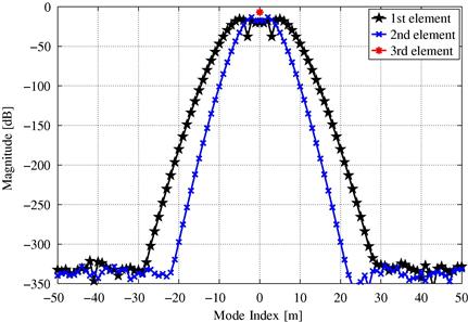
Figure 19.6 Three first rows of the array sampling matrix corresponding to the first three elements of the ideal ULA depicted in Figure 19.5. They represent the spatial Fourier coefficients of the first three array elements. The coefficients of the third array element are zero except at ![]() whereas that of the outer elements exhibit the superexponential property.
whereas that of the outer elements exhibit the superexponential property.

Figure 19.7 In (a) the norm of each column of the array sampling matrix for two ideal ULAs with different inter-element spacing. In (b) the average squared-residual of the manifold separation technique as a function of the number of modes. The saturation floor observed at ![]() is due to arithmetic precision of Matlab. The superexponential property of the array sampling matrix is a consequence of the finite aperture of sensor arrays.
is due to arithmetic precision of Matlab. The superexponential property of the array sampling matrix is a consequence of the finite aperture of sensor arrays.
The result in (19.27a and 19.27b) shows that the (noise-free) array output can be decomposed into two parts. One, represented by the array sampling matrix, characterizes the employed sensor array and it is independent of the wavefield. The second part, represented by the basis functions vector, characterizes the propagating wavefield and it is independent of the employed sensor array. In fact, a corollary of the wavefield modeling principle shows that the array steering vector may be decomposed as
![]() (19.28)
(19.28)
The result in (19.28) is known as manifold separation technique [18] and reveals an interesting interpretation for the array sampling matrix. It represents the spatial Fourier spectrum of the array steering vector
![]() (19.29)
(19.29)
where each row of the array sampling matrix contains the spatial Fourier coefficients of each array element. Hence, the array output (at each frequency) can be seen as the product between the spatial Fourier spectrum of the array steering vector and that of the propagating wavefield.
The array sampling matrix fully and uniquely characterizes a given sensor array since it contains the coefficients of an orthogonal spectral decomposition of the corresponding array steering vector. For example, ![]() contains information about the array configuration, sensors beampatterns (gain and phase response), mutual coupling, cross-polarization effects, mounting platform reflections, etc. In short, it contains all the effects that can be represented by the array steering vector
contains information about the array configuration, sensors beampatterns (gain and phase response), mutual coupling, cross-polarization effects, mounting platform reflections, etc. In short, it contains all the effects that can be represented by the array steering vector ![]() . Closed-form expressions for the array sampling matrix for some ideal sensor arrays can be found in [20]. However,
. Closed-form expressions for the array sampling matrix for some ideal sensor arrays can be found in [20]. However, ![]() may also be estimated in a non-parametric manner from array calibration measurements, without explicit formulations for the array nonidealities. In particular, the estimated array sampling matrix
may also be estimated in a non-parametric manner from array calibration measurements, without explicit formulations for the array nonidealities. In particular, the estimated array sampling matrix ![]() obtained as
obtained as
![]() (19.30a)
(19.30a)
![]() (19.30b)
(19.30b)
is known as effective aperture distribution function (EADF) [18,33]. In (19.30), ![]() denotes the unitary discrete Fourier transform (DFT) matrix and
denotes the unitary discrete Fourier transform (DFT) matrix and ![]() a selection matrix that optimally trades-off between complexity and accuracy of the resulting array steering vector model in (19.28).
a selection matrix that optimally trades-off between complexity and accuracy of the resulting array steering vector model in (19.28). ![]() may be estimated using state-of-the-art model order estimators [54].
may be estimated using state-of-the-art model order estimators [54].
We have mentioned that exact equality in (19.27b, 19.27a) and (19.28) requires that ![]() is composed of infinitely many columns.2 One may feel that such a requirement makes the wavefield modeling principle, or manifold separation technique, of theoretical interest only. The crucial property of the array sampling matrix that makes both wavefield modeling principle and manifold separation technique practical is known as superexponential decay. In particular, the magnitude of the columns of the sampling matrix,
is composed of infinitely many columns.2 One may feel that such a requirement makes the wavefield modeling principle, or manifold separation technique, of theoretical interest only. The crucial property of the array sampling matrix that makes both wavefield modeling principle and manifold separation technique practical is known as superexponential decay. In particular, the magnitude of the columns of the sampling matrix, ![]() , decay faster than exponential (i.e., superexponential) as
, decay faster than exponential (i.e., superexponential) as ![]() beyond
beyond ![]() .
. ![]() and r denote the angular wavenumber and radius of the smallest sphere enclosing the array structure (centered at the assumed coordinate system), respectively.
and r denote the angular wavenumber and radius of the smallest sphere enclosing the array structure (centered at the assumed coordinate system), respectively.
In practice, the superexponential property tells us that (19.27b, 19.27a) and (19.28) are (very) well approximated by a few columns ![]() of the array sampling matrix since the norm-convergence rate of the expansion in (19.28) is faster than exponential [18,20]; see Figure 19.7. The superexponential property may be understood by interpreting sensor arrays as spatial filters. In fact,
of the array sampling matrix since the norm-convergence rate of the expansion in (19.28) is faster than exponential [18,20]; see Figure 19.7. The superexponential property may be understood by interpreting sensor arrays as spatial filters. In fact, ![]() may be seen as the array’s spatial frequency response, where the passband, stopband, and cutoff frequencies are given by
may be seen as the array’s spatial frequency response, where the passband, stopband, and cutoff frequencies are given by ![]() , and
, and ![]() , respectively. For example, sensor arrays with large aperture have increased resolution since they sample the propagating wavefield over a large area. This is reflected on the array sampling matrix by an increase of the passband
, respectively. For example, sensor arrays with large aperture have increased resolution since they sample the propagating wavefield over a large area. This is reflected on the array sampling matrix by an increase of the passband ![]() (r increases). This leads to an increase of the amount of energy received from such a wavefield since a large number of wavefield coefficients
(r increases). This leads to an increase of the amount of energy received from such a wavefield since a large number of wavefield coefficients ![]() are taken into account by the employed sensor array.
are taken into account by the employed sensor array.
In the following, the main concepts and properties of wavefield modeling principle and manifold separation technique are illustrated using an ideal ULA. We emphasize that using ULAs does not limit the generality of the discussion. We employ it for the sake of clarity here. Let us consider the 5-element ULA from Figure 19.5, where the smallest sphere (a circle in this case) enclosing the array structure is depicted as well. Figure 19.6 illustrates three rows of the array sampling matrix, i.e., the spatial Fourier coefficients of the first three array elements. The ideal ULA is composed of omnidirectional elements with an inter-element spacing of ![]() . In Figure 19.7a, the norm of each column of the array sampling matrix,
. In Figure 19.7a, the norm of each column of the array sampling matrix, ![]() , is illustrated for two ideal ULAs with inter-element spacings of
, is illustrated for two ideal ULAs with inter-element spacings of ![]() and
and ![]() . Finally, Figure 19.7b, illustrates the following (average) squared-residual:
. Finally, Figure 19.7b, illustrates the following (average) squared-residual:
 (19.31)
as a function of ![]() , the number of columns of
, the number of columns of ![]() .
.
The simulation results show that the “passband” of the array sampling matrix increases for large apertures.3 In the limiting case of an infinitely small aperture, such as the omnidirectional array element located at the center of the coordinate system in Figure 19.5, the array sampling matrix is finite (see Figure 19.6). This is because only the magnitude response of such an array needs to be modeled (the first spatial harmonic in the case of omnidirectional elements) since the relative phase across such an aperture is zero.
A summary of the wavefield modeling principle/manifold separation technique is given in Table 19.5, where we assume that array calibration measurements are taken over the whole angular region, i.e., ![]() . We emphasize that such an assumption does not limit the generality of the wavefield modeling principle/manifold separation technique since it is simply related with the choice of orthogonal basis functions
. We emphasize that such an assumption does not limit the generality of the wavefield modeling principle/manifold separation technique since it is simply related with the choice of orthogonal basis functions ![]() , employed for decomposing the propagating wavefield. More precisely, wavefield modeling principle/manifold separation technique are also applicable when only partial array calibration measurements are acquired, or when the sources are known a priori to be confined to an angular sector. The superexponential property of the sampling matrix is also retained in such cases [20].
, employed for decomposing the propagating wavefield. More precisely, wavefield modeling principle/manifold separation technique are also applicable when only partial array calibration measurements are acquired, or when the sources are known a priori to be confined to an angular sector. The superexponential property of the sampling matrix is also retained in such cases [20].
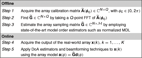
The wavefield modeling principle/manifold separation technique may also be employed as a complement to the auto-calibration techniques from Section 3.19.5 as well as to array interpolation technique and uncertainty sets (to be discussed in the next section). For example, in the case of uncertainties in the array elements’ positions, one may parameterize the array sampling matrix using the closed-form expressions in [20] and employ the auto-calibration techniques described in Section 3.19.5. The advantage of such an approach is the simplicity of using Fourier basis regardless of the configuration of the real-world array. One may also employ manifold separation technique with array interpolation technique to determine the conditions under which the real array output can be transformed to that of a virtual array, up to a specified mapping error [20]. Such conditions can be found with or without sector-by-sector processing. Finally, we note that many antenna measurement techniques, including the spherical near-field approach, are based on wavefield modeling [32,33]. This suggests that the wavefield modeling principle/manifold separation technique may play a fundamental role in any sensor array application.
3.19.7 Robust methods
Robust array processing procedures trade-off optimality to high reliability when the assumptions on the nominal signal or noise model do not hold [8,55–57]. The derivation of an optimal method is typically performed using strict assumptions on the sensor array model, propagation environment, source signals, as well as statistical properties of interference and noise. A shortcoming of the optimal array processing procedures is that they are extremely sensitive even to small deviations from the assumed model. In reality the underlying assumptions may not be valid and a significant degradation from the optimal performance is experienced.
Robust methods acknowledge that the assumptions on signal model may not be valid and do not try to recover the nonidealities from the observed or calibration data. Instead, they aim at bounding the influence of array modeling errors so that small departures from the nominal model lead only to small errors in the array processor output. One robust approach is based on minimax design which protects against a worst possible scenario, i.e., it is the best in the worst case. Hence, robust methods are also applicable if the conditions where the calibration was done are very different from the conditions where the sensor array system is deployed.
One simple approach is to assume that these errors are random, independent, and zero mean. Hence, they just decrease the SNR by increasing the noise variance. Since the array covariance matrix plays an important role in most array processing algorithms it is of interest to study how such a quantity behaves in nonstandard conditions. Assuming random errors, the perturbations may be expressed using the array covariance matrix as follows [58]:
![]()
where matrix ![]() is associated with errors that influence both the signal and noise components of the data. Departures from the nominal array response are included in the matrix
is associated with errors that influence both the signal and noise components of the data. Departures from the nominal array response are included in the matrix ![]() . This matrix contains the perturbations in element positions, errors in gain and phase responses of the sensors and mutual coupling. The term
. This matrix contains the perturbations in element positions, errors in gain and phase responses of the sensors and mutual coupling. The term ![]() describes the deviation of the noise covariance matrix from the nominal matrix
describes the deviation of the noise covariance matrix from the nominal matrix ![]() (noise is commonly assumed to be zero-mean complex-circular white Gaussian distributed and
(noise is commonly assumed to be zero-mean complex-circular white Gaussian distributed and ![]() an identity matrix). The effects of the above perturbations to high resolution DoA estimation as well as signal and noise subspaces may be studied using the first-order analysis introduced in [58] or by using tools from matrix perturbation theory. In the following, we will consider an example of robust beamforming that is optimized for the worst case scenario. A more detailed discussion can be found in chapter Adaptive and Robust Beamforming of this book.
an identity matrix). The effects of the above perturbations to high resolution DoA estimation as well as signal and noise subspaces may be studied using the first-order analysis introduced in [58] or by using tools from matrix perturbation theory. In the following, we will consider an example of robust beamforming that is optimized for the worst case scenario. A more detailed discussion can be found in chapter Adaptive and Robust Beamforming of this book.
3.19.7.1 Robust technique based on worst-case performance optimization and uncertainty sets
We have seen that steering vectors of real-world arrays are not exactly known in practice and that lack of knowledge or uncertainties about the array model may lead to a significant performance degradation in most array processors. For example, one may steer energy towards unwanted directions, cancel the SOI as well as amplify interfering sources or jammers; see Figure 19.8. The wavefield modeling principle/manifold separation technique aims at optimally describing (in the MSE sense, for example) nonidealities from array calibration measurements as well as incorporating such nonidealities into DoA estimators and beamforming techniques. However, real-world arrays may also be subject to nonidealities that change as a function of time or cannot be measured in controlled environments. For example, random fluctuations of the array response due to nearby scatterers or motion of the platform where the array is mounted are not captured in the calibration stage. In addition, imprecise knowledge of the DoAs may also lead to a performance degradation of beamforming techniques, a problem known as pointing angle or look direction errors. The idea of worst-case performance optimization techniques [59,60] employing so-called uncertainty sets [23,61], is to develop array processing techniques that are robust to general uncertainties in the steering vector of the real-world array.
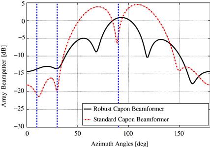
Figure 19.8 Example of array beampattern of both standard and robust Capon beamformer in case of steering vector uncertainties. The standard Capon beamformer cancels the SOI, located at ![]() .
.
Let us denote the exact (but unknown) steering vector of the real-world array by ![]() . Also, let
. Also, let ![]() denote the known but imprecise array steering vector, where
denote the known but imprecise array steering vector, where ![]() .
. ![]() may be acquired from array calibration measurements, EM simulation software or may represent an ideal ULA, for example. The vector
may be acquired from array calibration measurements, EM simulation software or may represent an ideal ULA, for example. The vector ![]() denotes the uncertainty we have about
denotes the uncertainty we have about ![]() and may be due to errors in pointing angle or imprecise gain of array elements. Worst-case performance optimization techniques proceed by assuming that the norm of the uncertainty vector can be bounded by a known
and may be due to errors in pointing angle or imprecise gain of array elements. Worst-case performance optimization techniques proceed by assuming that the norm of the uncertainty vector can be bounded by a known![]() such that
such that ![]() . This is equivalent to assuming that the imprecise steering vector
. This is equivalent to assuming that the imprecise steering vector ![]() belongs to a known hyper-ellipsoid centered at
belongs to a known hyper-ellipsoid centered at ![]() [23,61]:
[23,61]:
![]() (19.32)
(19.32)
Here, ![]() denotes a known positive-definite matrix that characterizes the shape of the ellipsoid and defines the maximum uncertainty we have about
denotes a known positive-definite matrix that characterizes the shape of the ellipsoid and defines the maximum uncertainty we have about ![]() . Ellipsoids of the form of (19.32) are called nondegenerate ellipsoids. If the uncertainty ellipsoids fall into a lower-dimensional space they are called flat (or degenerate) ellipsoids [61]. Flat ellipsoids are employed to make the uncertainty set as tight as possible but require more prior information about the maximum uncertainty than that of the nondegenerate ellipsoids.
. Ellipsoids of the form of (19.32) are called nondegenerate ellipsoids. If the uncertainty ellipsoids fall into a lower-dimensional space they are called flat (or degenerate) ellipsoids [61]. Flat ellipsoids are employed to make the uncertainty set as tight as possible but require more prior information about the maximum uncertainty than that of the nondegenerate ellipsoids.
Worst-case performance optimization techniques have been mostly used in the context of robust minimum variance beamforming [23,59–61]. The resulting robust beamformers can be shown to belong to the class of diagonal loading approaches. In fact, the optimal diagonal loading value can be found exactly from ![]() , unlike most of the ad hoc diagonal loading techniques [8]. However, the value of
, unlike most of the ad hoc diagonal loading techniques [8]. However, the value of ![]() and the shape of the uncertainty ellipsoid are typically specified by the designer. See e.g., [62] for alternative approaches to find the loading factor automatically.
and the shape of the uncertainty ellipsoid are typically specified by the designer. See e.g., [62] for alternative approaches to find the loading factor automatically.
Let us consider the eigenvalue decomposition of the sample covariance matrix ![]() , with
, with ![]() denoting the corresponding eigenvalues, and assume that
denoting the corresponding eigenvalues, and assume that ![]() . The array steering vector found by employing robust techniques based on uncertainty sets is [23]
. The array steering vector found by employing robust techniques based on uncertainty sets is [23]
![]() (19.33)
(19.33)
where ![]() is the solution of [23]
is the solution of [23]
 (19.34)
Here, ![]() and
and ![]() can be shown to belong to the following interval [23]
can be shown to belong to the following interval [23]
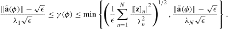 (19.35)
We may now use the steering vector model in (19.33) with the Capon beamformer expression from Section 3.19.2 in order to have a robust approach for both beamforming as well as DoA estimation. A summary of this robust technique is provided in Table 19.6.
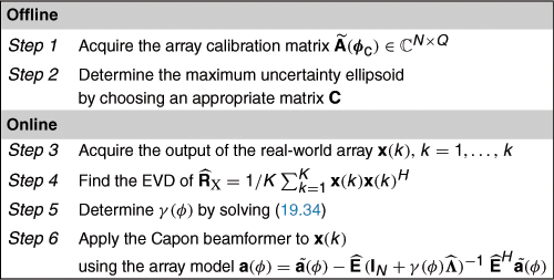
Typically, robust techniques based on uncertainty sets have a prohibitively large computational complexity. For example, the value ![]() in (19.33) needs to be found for every angle and may not be found offline since it is a function of
in (19.33) needs to be found for every angle and may not be found offline since it is a function of ![]() . An exception that is worth mentioning is the robust beamformer of [60], where the beamformer weights may be updated snapshot-by-snapshot using subspace tracking techniques. However, such an approach is still not practical in DoA estimation since it requires finding a principal eigenvector for each grid point of the spectral search.
. An exception that is worth mentioning is the robust beamformer of [60], where the beamformer weights may be updated snapshot-by-snapshot using subspace tracking techniques. However, such an approach is still not practical in DoA estimation since it requires finding a principal eigenvector for each grid point of the spectral search.
3.19.8 Array processing examples
3.19.8.1 DoA estimation using an ideal uniform linear array and manifold separation technique
Let us consider that a propagating wavefield, generated by two equi-power and uncorrelated point-sources, impinge on an ideal ULA from ![]() , measured from the endfire of the array. The ULA is composed of 5 omnidirectional elements with an inter-element spacing of
, measured from the endfire of the array. The ULA is composed of 5 omnidirectional elements with an inter-element spacing of ![]() . We employ the root-MUSIC [63] and element-space (ES) root-MUSIC [18] algorithms. Since the employed sensor array is composed of omnidirectional elements the array sampling matrix
. We employ the root-MUSIC [63] and element-space (ES) root-MUSIC [18] algorithms. Since the employed sensor array is composed of omnidirectional elements the array sampling matrix ![]() may be found in a closed-form [20]. Figure 19.9 illustrates the performance of both root-MUSIC and ES root-MUSIC algorithms in terms of root mean-squared error (RMSE). Only the results for
may be found in a closed-form [20]. Figure 19.9 illustrates the performance of both root-MUSIC and ES root-MUSIC algorithms in terms of root mean-squared error (RMSE). Only the results for ![]() are illustrated but similar results are obtained for
are illustrated but similar results are obtained for ![]() . Figure 19.9a illustrates the RMSE as a function of snapshots, with
. Figure 19.9a illustrates the RMSE as a function of snapshots, with ![]() , while Figure 19.9b illustrates the RMSE as a function of SNR, with
, while Figure 19.9b illustrates the RMSE as a function of SNR, with ![]() snapshots. The number of columns of
snapshots. The number of columns of ![]() employed by the ES root-MUSIC is
employed by the ES root-MUSIC is ![]() . Results show that the ES root-MUSIC has a performance very close to the root-MUSIC even though the former employs an approximation of the array steering vector.
. Results show that the ES root-MUSIC has a performance very close to the root-MUSIC even though the former employs an approximation of the array steering vector.
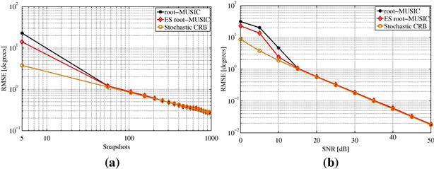
Figure 19.9 Performance of both standard root-MUSIC and ES root-MUSIC algorithms as a function of (a) snapshots and (b) SNR. A propagating wavefield, generated by two equi-power and uncorrelated sources, impinge on an ideal ULA from ![]() . Only the results for
. Only the results for ![]() are illustrated but similar results are obtained for
are illustrated but similar results are obtained for ![]() . The number of columns of
. The number of columns of ![]() employed by the ES root-MUSIC is
employed by the ES root-MUSIC is ![]() . Results show that there is practically no loss of performance, even though the ES root-MUSIC employs an approximation of the array steering vector.
. Results show that there is practically no loss of performance, even though the ES root-MUSIC employs an approximation of the array steering vector.
The complexity of the ES root-MUSIC is, of course, higher than that of the root-MUSIC algorithm, and if the employed sensor array is indeed an ideal ULA one should resort to the standard root-MUSIC algorithm. However, if the task is estimate DoAs using real-world arrays with imperfections, the ES root-MUSIC is a very attractive choice. Note that the complexity of the ES root-MUSIC algorithm may be reduced by means of Schur factorization and Arnoldi iterations [64].
Let us now suppose that the only information we have about a real-world array is by means of its array measurement matrix ![]() , and the stochastic CRB expression for array processing in (19.9) needs to be found. One may employ the manifold separation technique in (19.28) with (19.9) in order to find an approximate CRB expression that is tight even for real-world arrays with nonidealities, excluding the low SNR regime where the CRB is not a tight bound in general. To illustrate this, let us assume that the array measurement matrix of the 5-element ULA from Figure 19.5 is obtained from
, and the stochastic CRB expression for array processing in (19.9) needs to be found. One may employ the manifold separation technique in (19.28) with (19.9) in order to find an approximate CRB expression that is tight even for real-world arrays with nonidealities, excluding the low SNR regime where the CRB is not a tight bound in general. To illustrate this, let us assume that the array measurement matrix of the 5-element ULA from Figure 19.5 is obtained from ![]() points
points ![]() with
with ![]() . The EADF of such an ULA is obtained from the array measurement matrix using Eq. (19.30). The resulting array steering vector model, Eq. (19.28), is employed with the CRB expression in (19.9) in order to obtain an approximate CRB expression. Figure 19.10 illustrates the ratio between the approximate and exact stochastic CRBs as a function of the number of columns of
. The EADF of such an ULA is obtained from the array measurement matrix using Eq. (19.30). The resulting array steering vector model, Eq. (19.28), is employed with the CRB expression in (19.9) in order to obtain an approximate CRB expression. Figure 19.10 illustrates the ratio between the approximate and exact stochastic CRBs as a function of the number of columns of ![]() . The results have been averaged over
. The results have been averaged over ![]() and 100 realizations of calibration noise. The approximate CRB expression obtained by employing the manifold separation principle is accurate since the ratio
and 100 realizations of calibration noise. The approximate CRB expression obtained by employing the manifold separation principle is accurate since the ratio ![]() converges to unity. We also note that the accuracy of the approximate CRB expression is related to the electrical dimension of the employed sensor array. In fact, the ratio
converges to unity. We also note that the accuracy of the approximate CRB expression is related to the electrical dimension of the employed sensor array. In fact, the ratio ![]() converges to unity around
converges to unity around ![]() modes which, as discussed in Section 3.19.6, is the point where the magnitude of the array sampling matrix starts decaying superexponentially.
modes which, as discussed in Section 3.19.6, is the point where the magnitude of the array sampling matrix starts decaying superexponentially.
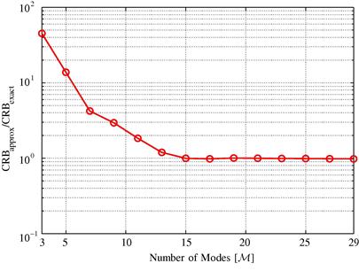
Figure 19.10 Accuracy of the approximate CRB expression obtained by employing the manifold separation technique. The ratio between the approximate and exact CRBs is illustrated as a function of the number of columns of the EADF. The approximate CRB expression is accurate since the ratio ![]() converges to one around
converges to one around ![]() , which is a measure of the electrical dimension of the employed sensor array. The approximate CRB expression obtained by employing the manifold separation technique is tight and very useful for real-world arrays with imperfections.
, which is a measure of the electrical dimension of the employed sensor array. The approximate CRB expression obtained by employing the manifold separation technique is tight and very useful for real-world arrays with imperfections.
3.19.8.2 Robust beamforming using array calibration
Let us consider that a propagating wavefield, generated by three uncorrelated point-sources, impinge on an ideal ULA that is identical to the one employed in the previous example. The SOI and interfering sources impinge on the sensor array from ![]() and
and ![]() , respectively. The signal powers of the interferers are
, respectively. The signal powers of the interferers are ![]() . We consider two sources of uncertainty in the array steering vector
. We consider two sources of uncertainty in the array steering vector ![]() , namely due to array calibration noise and error in the look direction. In particular, we employ the array measurement matrix
, namely due to array calibration noise and error in the look direction. In particular, we employ the array measurement matrix ![]() of the ULA, found with an
of the ULA, found with an ![]() and
and ![]() calibration points. In addition, we consider that there is an error of two degrees in the DoA of the SOI. We employ the robust Capon beamformer, obtained by using (19.33) in (19.7), with the imprecise array steering vector
calibration points. In addition, we consider that there is an error of two degrees in the DoA of the SOI. We employ the robust Capon beamformer, obtained by using (19.33) in (19.7), with the imprecise array steering vector ![]() found directly from
found directly from ![]() , and by employing the manifold separation technique, i.e., using the EADF
, and by employing the manifold separation technique, i.e., using the EADF ![]() . The uncertainty ellipsoid is fixed with
. The uncertainty ellipsoid is fixed with ![]() , where
, where ![]() . Figure 19.11a illustrates the array output SINR as a function of snapshots with
. Figure 19.11a illustrates the array output SINR as a function of snapshots with ![]() while Figure 19.11b illustrates the array output SINR as a function of the SNR of the SOI with
while Figure 19.11b illustrates the array output SINR as a function of the SNR of the SOI with ![]() snapshots. Employing the manifold separation technique leads to improved performance since it attenuates calibration measurement noise [18].
snapshots. Employing the manifold separation technique leads to improved performance since it attenuates calibration measurement noise [18].

Figure 19.11 Performance of the robust beamformer based on uncertainty sets in terms of (a) array output SINR as a function of snapshots and (b) array output SINR as a function of SNR of the SOI. Two sources of uncertainty in the array steering vector are considered, namely due to array calibration noise and error in the look direction. Employing the manifold separation technique leads to improved performance since it allows reducing calibration measurement noise while modeling array nonidealities.
3.19.8.3 Polynomial rooting techniques for real-world arrays with nonidealities
Let us now consider DoA estimation algorithms based on polynomial rooting techniques that can be employed regardless of the array configuration and nonidealities. Assume that a propagating wavefield, generated by two point-sources, is observed by the real-world array from Figure 19.12[65]. The sources are located in the far-field of the sensor array and their DoAs are ![]() . The sources are assumed to be located in the same plane (xy-plane) as the employed antenna array. Only the array measurement matrix
. The sources are assumed to be located in the same plane (xy-plane) as the employed antenna array. Only the array measurement matrix ![]() of the real-world array is known. The interpolated root-MUSIC algorithm [15] as well as the ES root-MUSIC [18] and the Fourier-domain (FD) root-MUSIC [50] are used to provide the angle estimates as follows.
of the real-world array is known. The interpolated root-MUSIC algorithm [15] as well as the ES root-MUSIC [18] and the Fourier-domain (FD) root-MUSIC [50] are used to provide the angle estimates as follows.
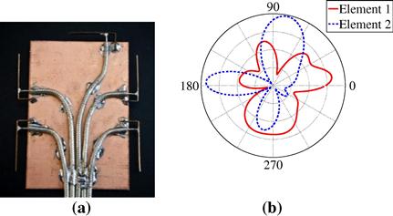
Figure 19.12 (a) Five-element Inverted-F Antenna (IFA) array built for direction-finding purposes using handheld terminals. Its dimensions, center frequency and bandwidth are ![]()
![]() , and
, and ![]() , respectively. (b) Magnitude of the radiation pattern of two elements of the array. Each antenna has a different radiation characteristic which is far from the ideal omnidirectional pattern. Courtesy of the Department of Radio Science and Technology, Aalto University, Finland.
, respectively. (b) Magnitude of the radiation pattern of two elements of the array. Each antenna has a different radiation characteristic which is far from the ideal omnidirectional pattern. Courtesy of the Department of Radio Science and Technology, Aalto University, Finland.
The interpolated root-MUSIC algorithm is employed by first determining 12 array mapping matrices ![]() , one for each
, one for each ![]() -sector, from
-sector, from ![]() . Each of the 12 virtual ULAs (one per sector) is located at the center of the minimum circle enclosing the employed sensor array and oriented so that its broadside corresponds to the middle of each sector. The virtual ULAs are composed of five elements with an inter-element spacing of
. Each of the 12 virtual ULAs (one per sector) is located at the center of the minimum circle enclosing the employed sensor array and oriented so that its broadside corresponds to the middle of each sector. The virtual ULAs are composed of five elements with an inter-element spacing of ![]() , so that the aperture of the virtual ULAs is maximized while guaranteeing a small condition number of the mapping matrices. The remaining steps of the interpolated root-MUSIC algorithm are implemented as described in [15].
, so that the aperture of the virtual ULAs is maximized while guaranteeing a small condition number of the mapping matrices. The remaining steps of the interpolated root-MUSIC algorithm are implemented as described in [15].
The ES root-MUSIC algorithm is implemented by first determining the EADF, denoted by ![]() as described in (16.6.9). This includes taking the FFT of the array measurement matrix and determining the number of columns
as described in (16.6.9). This includes taking the FFT of the array measurement matrix and determining the number of columns ![]() by means of a model order estimation technique such as MDL [54]. After determining the noise subspace
by means of a model order estimation technique such as MDL [54]. After determining the noise subspace ![]() of the sample covariance matrix
of the sample covariance matrix ![]() , the DoA estimates are found from the phase-angles of the P roots closest to the unit circle (either inside of outside the unit circle) of the following polynomial
, the DoA estimates are found from the phase-angles of the P roots closest to the unit circle (either inside of outside the unit circle) of the following polynomial
![]() (19.36)
(19.36)
Note that the coefficients in (19.36) may be found in a computationally efficient manner using the FFT:
 (19.37)
where ![]() .
.
The FD root-MUSIC algorithm is implemented by first determining the sampled MUSIC nullspectrum ![]() :
:
![]() (19.38)
(19.38)
Then, the coefficients of the FD root-MUSIC polynomial
![]() (19.39)
(19.39)
are obtained as
![]() (19.40a)
(19.40a)
![]() (19.40b)
(19.40b)
where ![]() and the selection matrix
and the selection matrix ![]() is obtained in a similar fashion as with the ES root-MUSIC.
is obtained in a similar fashion as with the ES root-MUSIC.
Figure 19.13 illustrates the performance of the three polynomial rooting approaches in terms of RMSE as a function of (a) snapshots with ![]() and (b) SNR with
and (b) SNR with ![]() snapshots. Only the results for
snapshots. Only the results for ![]() are shown but similar results are obtained for
are shown but similar results are obtained for ![]() . The algorithms exploit a noise-free array measurement matrix with
. The algorithms exploit a noise-free array measurement matrix with ![]() calibration points. The degree of both ES root-MUSIC and FD root-MUSIC polynomials are equal with
calibration points. The degree of both ES root-MUSIC and FD root-MUSIC polynomials are equal with ![]() . Results show that the ES root-MUSIC as well as the FD root-MUSIC have similar performance and are closed to the stochastic CRB while the estimates obtained by the interpolated root-MUSIC have large bias and excess variance.
. Results show that the ES root-MUSIC as well as the FD root-MUSIC have similar performance and are closed to the stochastic CRB while the estimates obtained by the interpolated root-MUSIC have large bias and excess variance.
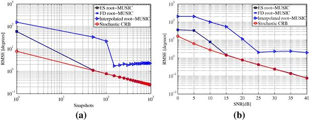
Figure 19.13 Performance of interpolated root-MUSIC, ES root-MUSIC, and FD root-MUSIC algorithms as a function of (a) snapshots and (b) SNR. A propagating wavefield, generated by two equi-power and uncorrelated sources located at ![]() , impinge the sensor array from Figure 19.12. Only the results for
, impinge the sensor array from Figure 19.12. Only the results for ![]() are illustrated but similar results are obtained for
are illustrated but similar results are obtained for ![]() . The array calibration matrix is noise-free and
. The array calibration matrix is noise-free and ![]() points have been taken. Results show that the ES root-MUSIC as well as the FD root-MUSIC have similar performance and are closed to the stochastic CRB while the estimates obtained by the interpolated root-MUSIC have large bias and excess variance.
points have been taken. Results show that the ES root-MUSIC as well as the FD root-MUSIC have similar performance and are closed to the stochastic CRB while the estimates obtained by the interpolated root-MUSIC have large bias and excess variance.
Figure 19.14 illustrates the sensitivity of both ES root-MUSIC and FD root-MUSIC algorithms, for a fixed ![]() , to (a) calibration SNR (
, to (a) calibration SNR (![]() ) with
) with ![]() and (b) calibration points Q with
and (b) calibration points Q with ![]() . Two equi-power sources impinge on the 5-element IFA array from
. Two equi-power sources impinge on the 5-element IFA array from ![]() with an
with an ![]() and
and ![]() . Only the results for
. Only the results for ![]() are illustrated but similar results are obtained for
are illustrated but similar results are obtained for ![]() . Results show that the ES root-MUSIC algorithm outperforms the FD root-MUSIC when the array measurement matrix is corrupted by calibration noise.
. Results show that the ES root-MUSIC algorithm outperforms the FD root-MUSIC when the array measurement matrix is corrupted by calibration noise.
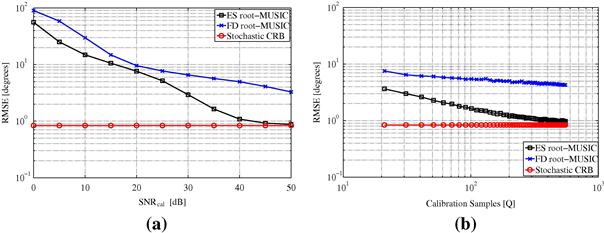
Figure 19.14 Sensitivity of ES root-MUSIC and FD root-MUSIC algorithms, with a fixed ![]() , to (a) calibration SNR (
, to (a) calibration SNR (![]() ) with
) with ![]() and (b) number of calibration points Q with
and (b) number of calibration points Q with ![]() . Two equi-power sources impinge on the 5-element IFA array from
. Two equi-power sources impinge on the 5-element IFA array from ![]() with an
with an ![]() and
and ![]() . Results show that the ES root-MUSIC algorithm outperforms the FD root-MUSIC when the array measurement matrix is corrupted by calibration noise.
. Results show that the ES root-MUSIC algorithm outperforms the FD root-MUSIC when the array measurement matrix is corrupted by calibration noise.
3.19.8.4 Azimuth, elevation, and polarization estimation
Let us now consider the general case of estimating both azimuth ![]() and elevation
and elevation ![]() angles of a completely polarized EM propagating wavefield. Typically, the polarization of the wavefield is unknown and needs to be estimated along with the DoAs. The narrowband array output model is now given by
angles of a completely polarized EM propagating wavefield. Typically, the polarization of the wavefield is unknown and needs to be estimated along with the DoAs. The narrowband array output model is now given by
![]() (19.41)
(19.41)
where ![]() denote the array steering matrices due to a vertical and horizontal polarized wavefields, respectively.
denote the array steering matrices due to a vertical and horizontal polarized wavefields, respectively. ![]() describes the polarization of the wavefield and it is typically given by
describes the polarization of the wavefield and it is typically given by
![]() (19.42a)
(19.42a)
![]() (19.42b)
(19.42b)
where ![]() and
and ![]() . The parameters
. The parameters ![]() and
and ![]() describe the polarization ellipse of the received Electric-field and take values over
describe the polarization ellipse of the received Electric-field and take values over ![]() and
and ![]() , respectively. The techniques described in Sections 3.19.5 and 3.19.6 may now be employed to (19.41) by modeling the array steering vector
, respectively. The techniques described in Sections 3.19.5 and 3.19.6 may now be employed to (19.41) by modeling the array steering vector ![]() either in a parametric or non-parametric manner.
either in a parametric or non-parametric manner.
In particular, the wavefield modeling principle/manifold separation technique for completely polarized EM wavefields consists in employing so-called vector spherical harmonics, instead of Fourier basis in (19.27b, 19.27a) and (19.28). The motivation for using vector spherical harmonics follows from the fact that such basis functions form a complete and orthonormal set on the 2-sphere, similarly to Fourier basis in azimuth-only processing. However, vector spherical harmonics, which have a rather cumbersome algebraic form, are less attractive than Fourier basis for the purposes of array processing and may be subject to numerical instabilities. In fact, a formulation of the wavefield modeling principle/manifold separation technique involving 2-D Fourier basis may be found in [53], where it is employed the so-called equivalence matrix [19]. A summary of the wavefield modeling principle/manifold separation technique for completely polarized EM wavefields is given in Table 19.7.
Table 19.7
Steps of Wavefield Modeling Principle/Manifold Separation Technique for Completely Polarized EM Wavefields
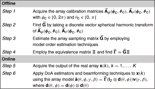
Let us consider that a propagating EM wavefield, generated by two equi-power far-field point-sources, is received by the 5-element IFA from Figure 19.12. The DoAs and polarization parameters are ![]() ,
, ![]() , and
, and ![]() , respectively.
, respectively. ![]() snapshots are acquired at the array output. The array response was obtained from an EM simulation software; see [65] for details. The manifold separation technique is employed for determining the array steering vector model along with its nonidealities, as described in Table 19.7. The polarimetric element-space (PES) MUSIC algorithm [53] is used for estimating both DoAs and polarization parameters of the sources generating the wavefield.
snapshots are acquired at the array output. The array response was obtained from an EM simulation software; see [65] for details. The manifold separation technique is employed for determining the array steering vector model along with its nonidealities, as described in Table 19.7. The polarimetric element-space (PES) MUSIC algorithm [53] is used for estimating both DoAs and polarization parameters of the sources generating the wavefield.
Figure 19.15 illustrates the statistical performance of the PES MUSIC in terms of RMSE as a function of SNR. Only the angle estimates are shown but similar results are obtained for the polarization parameters. Results show that the PES MUSIC algorithm has a performance close to the stochastic CRB since it takes into account array nonidealities.

Figure 19.15 Statistical performance of the PES MUSIC algorithm using the 5-element IFA from Figure 19.12. The DoAs and polarization parameters are ![]()
![]()
![]()
![]() and
and ![]()
![]()
![]()
![]() , respectively. The PES MUSIC algorithm takes into account array nonidealities and has a performance close to the stochastic CRB.
, respectively. The PES MUSIC algorithm takes into account array nonidealities and has a performance close to the stochastic CRB.
3.19.9 Conclusion
In this chapter, array signal processing in face of array nonidealities was addressed. Real-world arrays are always subject to nonidealities such as mutual coupling, mounting platform reflections, cross-polarization effects, sensors with individual beampatterns as well as sensors’ position errors. We have seen that such nonidealities typically lead to a significant performance degradation as well as loss of optimality of DoA estimators and beamforming techniques.
Various techniques for dealing with array nonidealities have been described. They are classified as model-driven techniques, data-driven, and robust methods. Model-driven techniques use an explicit formulation describing each nonideality, which may be challenging to specify, and include auto-calibration techniques as well as so-called parametric calibration methods. Data-driven techniques do not assume any explicit formulation for the nonidealities but employ array calibration measurements. They capture the nonidealities implicitly by using basis function expansion, interpolation, approximation or nonparameteric estimation techniques. Data-driven techniques include local interpolation of the array calibration matrix, array interpolation as well as manifold separation techniques. Finally, robust methods try to bound the influence of nonidealities in the estimation process instead of trying to capture them. Typically, robust methods trade-off optimality for reliability.
Extensive array processing examples have been included. They explain in detail how array processing techniques may deal with array nonidealities by employing data-driven techniques as well as robust methods.
We note that the various techniques for dealing with array nonidealities described in this chapter have different features and may complement each other. Future research work may thus be based on combining auto-calibration techniques and robust methods with manifold separation.
Relevant Theory: Signal Processing Theory, Statistical Signal Processing and Array Signal Processing
See Vol. 1, Chapter 11 Parametric Estimation
See this Volume, Chapter 2 Model Order Selection
See this Volume, Chapter 16 Performance Bounds and Statistical Analysis of DOA Estimation
References
1. Stoica P, Moses R. Introduction to Spectral Analysis. Wiley 1997.
2. Krim H, Viberg M. Two decades of array signal processing. IEEE Signal Process Mag. 1996;67–94.
3. Wijnholds S, van der Tol S, Nijboer R, van der Veen A. Calibration challenges for future radio telescopes. IEEE Signal Process Mag. 2010;27(1):30–42.
4. Gesbert D, van Rensburg C, Tosato F, Kaltenberger F. Multiple antenna techniques. In: Sesia S, Toufik I, Baker M, eds. LTE—The UMTS Long Term Evolution: From Theory to Practice. John Wiley and Sons 2009;243–283. (Chapter 11).
5. Belloni F, Ranki V, Kainulainen A, Richter A. Angle-based indoor positioning system for open indoor environments. In: Workshop on Positioning, Navigation and, Communication. 2009;261–265.
6. Viberg M, Lanne M, Lundgren A. Calibration in array processing. In: Tuncer T, Friedlander B, eds. Classical and Modern Direction-of-Arrival Estimation. Burlington, MA, USA: Academic Press; 2009;93–124. (Chapter 3).
7. Jansson M, Swindlehurst A, Ottersten B. Weighted subspace fitting for general array error models. IEEE Trans Signal Process. 1998;46(9):2484–2498.
8. Gershman A. Robust adaptive beamforming in sensor arrays. Int J Electron Commun. 1999;53(6):305–314.
9. Mailloux R. Array failure correction with a digitally beamformed array. IEEE Trans Antennas Propag. 1996;44(12):1543–1550.
10. Waters A, Cevher V. Distributed bearing estimation via matrix completion. In: Proceedings of the IEEE International Conference on Acoustics, Speech, and, Signal Processing. 2010;2590–2593.
11. Weiss A, Friedlander B. Eigenstructure methods for direction finding with sensor gain and phase uncertainties. Circ Syst Signal Process. 1990;9(3):271–300.
12. Weiss A, Friedlander B. Array shape calibration using sources in unknown locations—a maximum likelihood approach. IEEE Trans Acoust Speech Signal Process. 1989;37(12):1958–1966.
13. Rockah Y, Schultheiss P. Array shape calibration using sources in unknown locations—Part I: far-field sources. IEEE Trans Acoust Speech Signal Process. 1987;35(3):286–299.
14. Viberg M, Swindlehurst A. A Bayesian approach to auto-calibration for parametric array signal processing. IEEE Trans Signal Process. 1994;42(12):3495–3507.
15. Friedlander B. The root-MUSIC algorithm for direction finding with interpolated arrays. Signal Process. 1993;30:15–19.
16. Hyberg P, Jansson M, Ottersten B. Array interpolation and DOA MSE reduction. IEEE Trans Signal Process. 2005;53(12):4464–4471.
17. Gershman A, Böhme J. A note on most favorable array geometries for DOA estimation and array interpolation. IEEE Signal Process Lett. 1997;4(8):232–235.
18. Belloni F, Richter A, Koivunen V. DoA estimation via manifold separation for arbitrary array structures. IEEE Trans Signal Process. 2007;55(10):4800–4810.
19. Costa M, Richter A, Koivunen V. Unified array manifold decomposition based on spherical harmonics and 2-D Fourier basis. IEEE Trans Signal Process. 2010;58(9):4634–4645.
20. Doron M, Doron E. Wavefield modeling and array processing, Part I—Spatial sampling. IEEE Trans Signal Process. 1994;42(10):2549–2559.
21. Doron M, Doron E. Wavefield modeling and array processing, Part II—Algorithms. IEEE Trans Signal Process. 1994;42(10):2560–2570.
22. Doron M, Doron E. Wavefield modeling and array processing, Part III—Resolution capacity. IEEE Trans Signal Process. 1994;42(10):2571–2580.
23. Li J, Stoica P, Wang Z. On robust Capon beamforming and diagonal loading. IEEE Trans Signal Process. 2003;51(7):1702–1715.
24. Kay S. Fundamentals of Statistical Signal Processing: Estimation Theory. Prentice Hall 1993.
25. Stoica P, Larsson E, Gershman A. The stochastic CRB for array processing: a textbook derivation. IEEE Signal Process Lett. 2001;8(5):148–150.
26. Stoica P, Ottersten B, Viberg M, Moses R. Maximum likelihood array processing for stochastic coherent sources. IEEE Trans Signal Process. 1996;44(1):96–105.
27. Koivunen V, Ollila E. Direction of arrival estimation under uncertainty. In: Chandran S, ed. Advances in Direction of Arrival Estimation. Artech House 2006;241–258. (Chapter 12).
28. Mailloux R. Phased Array Antenna Handbook. second ed. Artech House 2005.
29. Dandekar K, Ling H, Xu G. Effect of mutual coupling on direction finding in smart antenna applications. Electron Lett. 2000;36(22):1889–1891.
30. Goossens R, Rogier H. A hybrid UCA-RARE/root-MUSIC approach for 2-D direction of arrival estimation in uniform circular arrays in the presence of mutual coupling. IEEE Trans Antennas Propag. 2007;55(3):841–849.
31. Steyskal H, Herd J. Mutual coupling compensation in small array antennas. IEEE Trans Antennas Propag. 1990;38(12):1971–1975.
32. Hansen J, ed. Spherical Near-Field Antenna Measurements. Peter Peregrinus Ltd. 1988.
33. Landmann M, Käske M, Thomä R. Impact of incomplete and inaccurate data models on high resolution parameter estimation in multidimensional channel sounding. IEEE Trans Antennas Propag. 2012;60(2):557–573.
34. Zatman M. How narrowband is narrowband? IEE Proc Radar Sonar Navig. 1998;145(2):85–91.
35. Wang H, Kaveh M. Coherent signal-subspace processing for the detection and estimation of angles of arrival of multiple wide-band sources. IEEE Trans Acoust Speech Signal Process. 1985;33(4):823–831.
36. Klemm R. Principles of Space-Time Adaptive Processing. The Institution of Electrical Engineers 2002.
37. Werner S, With M, Koivunen V. Householder multistage Wiener filter for space-time navigation receivers. IEEE Trans Aerosp Electron Syst. 2007;43(3):975–988.
38. Sorelius J, Moses R, Söderström T, Swindlehurst A. Effects of nonzero bandwidth on direction of arrival estimators in array signal processing. IEE Proc Radar Sonar Navig. 1998;145(6):317–324.
39. Abidi A. Direct-conversion radio transceivers for digital communications. IEEE J Solid State Circ. 1995;30(12):1399–1410.
40. Nickel U. On the influence of channel errors on array signal processing methods. Int J Electron Commun. 1993;47(4):209–219.
41. Demmel F. Practical aspects of design and application of direction-finding systems. In: Tuncer T, Friedlander B, eds. Classical and Modern Direction-of-Arrival Estimation. Burlington, MA, USA: Academic Press; 2009;53–92.
42. Krishnamurthy G, Gard K. Time division multiplexing front-ends for multiantenna integrated wireless receivers. IEEE Trans Circ Syst I: Regular Papers. 2010;57(6):1231–1243.
43. Loyka S. The influence of electromagnetic environment on operation of active array antennas: analysis and simulation techniques. IEEE Antennas Propag Mag. 1999;41(6):23–39.
44. Valkama M, Springer A, Hueber G. Digital signal processing for reducing the effects of RF imperfections in radio devices—an overview. In: Proceedings of the IEEE International Symposium on Circuits and Systems. 2010;813–816.
45. Toivanen J, Laitinen T, Vainikainen P. Modified test zone field compensation for small-antenna measurements. IEEE Trans Antennas Propag. 2010;58(11):3471–3479.
46. Golub G, Loan C. Matrix Computations. third ed. John Hopkins University Press 1996.
47. Fessler J, Hero A. Space-alternating generalized expectation-maximization algorithm. IEEE Trans Signal Process. 1994;42(10):2664–2677.
48. Stoica P, Sharman K. Maximum likelihood methods for direction-of-arrival estimation. IEEE Trans Acoust Speech Signal Process. 1990;38(7):1132–1143.
49. Viberg M, Ottersten B. Sensor array processing based on subspace fitting. IEEE Trans Signal Process. 1991;39(5):1110–1121.
50. Rübsamen M, Gershman A. Direction-of-arrival estimation for nonuniform sensor arrays: from manifold separation to Fourier domain MUSIC methods. IEEE Trans Signal Process. 2009;57(2):588–599.
51. Mathews C, Zoltowski M. Eigenstructure techniques for 2-D angle estimation with uniform circular arrays. IEEE Trans Signal Process. 1994;42(9):2395–2407.
52. Pesavento M, Gershman A, Luo Z. Robust array interpolation using second-order cone programming. IEEE Signal Process Lett. 2002;9(1):8–11.
53. Costa M, Richter A, Koivunen V. DoA and polarization estimation for arbitrary array configurations. IEEE Trans Signal Process. 2012;60(5):2330–2343.
54. Rissanen J. MDL denoising. IEEE Trans Inform Theory. 2000;46(7):2537–2543.
55. Li J, Stoica P, eds. Robust Adaptive Beamforming. John Wiley and Sons 2006.
56. Zoubir A, Koivunen V, Chakhchoukh Y, Muma M. Robust estimation in signal processing. IEEE Signal Process Mag. 2012;29.
57. Ollila E, Koivunen V. Robust estimation techniques for complex-valued random vectors. In: Haykin S, Adali T, eds. Adaptive Signal Processing: Next Generation Solutions. Wiley 2009;87–142.
58. Swindlehurst A, Kailath T. A performance analysis of subspace-based methods in the presence of model errors—Part I: the MUSIC algorithm. IEEE Trans Signal Process. 1992;40(7):1758–1774.
59. Vorobyov S, Gershman A, Luo Z. Robust adaptive beamforming using worst-case performance optimization: a solution to the signal mismatch problem. IEEE Trans Signal Process. 2003;51(2):313–324.
60. Shahbazpanahi S, Gershman A, Luo Z, Wong K. Robust adaptive beamforming for general-rank signal models. IEEE Trans Signal Process. 2003;51(9):2257–2269.
61. Lorenz R, Boyd S. Robust minimum variance beamforming. IEEE Trans Signal Process. 2005;53(5):1684–1696.
62. Du L, Yardibi T, Li J, Stoica P. Review of user parameter-free robust adaptive beamforming algorithms. Digit Signal Process. 2009;19(4):567–582.
63. Barabell A. Improving the resolution performance of the eigenstructure-based direction-finding algorithms. In: IEEE International Conference on Acoustics, Speech and Signal Processing. 1983;336–339.
64. Zhuang J, Li W, Manikas A. Fast root-MUSIC for arbitrary arrays. Electron Lett. 2010;46(2):174–176.
65. Azremi A, Kyro M, Ilvonen J, et al. Five-element inverted-F antenna array for MIMO communications and radio direction finding on mobile terminal. In: Loughborough Antennas and Propagation Conference. 2009;557–560.
1This may be alleviated by means of uncertainty sets on the array steering vector, to be discussed in Section 3.19.7. For example, uncertainties in the array elements’ locations may be bounded by the array aperture, thus avoiding the difficulties that may arise in deriving Bayesian type of estimators with truncated prior distributions.
2In the limiting case of an infinitely small aperture the array sampling matrix is finite.
3The correct term should be electric dimensions since the superexponential property is inversely proportional to the wavelength, in addition to the relationship with the physical dimension of the array.