
Vortex sound
Abstract
One of the concerns with Lighthill's analogy is the physical interpretation of the source term Tij and relating it to easily recognized features of the flow. In many cases the flow may include relatively large coherent structures that are characterized by almost two-dimensional line vortices. Examples include coherent vortex shedding behind a cylinder or into a wake, and tip vortices interacting with helicopter rotor blades. These problems are often more readily understood if the sound is related to the vorticity in the flow rather than the Lighthill stress tensor. In this chapter we review the theory of vortex sound and give some examples of its application in low Mach number flows. In particular we will consider the sound radiation caused by the unsteady loading on rigid, acoustically compact surfaces in the presence of flows that can be modeled by coherent vortical structures.
Keywords
Vortex sound; Spinning vortices; Aeolian tones; Unsteady loads in incompressible flow; Blade vortex interaction in incompressible flow; Angle of attack
One of the concerns with Lighthill's analogy is the physical interpretation of the source term Tij and relating it to easily recognized features of the flow. In many cases the flow may include relatively large coherent structures that are characterized by almost two-dimensional line vortices. Examples include coherent vortex shedding behind a cylinder or into a wake, and tip vortices interacting with helicopter rotor blades. These problems are often more readily understood if the sound is related to the vorticity in the flow rather than the Lighthill stress tensor. In this chapter we review the theory of vortex sound and give some examples of its application in low Mach number flows. In particular we will consider the sound radiation caused by the unsteady loading on rigid, acoustically compact surfaces in the presence of flows that can be modeled by coherent vortical structures.
7.1 Theory of vortex sound
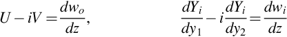
The theory of vortex sound was first discussed by Powell [1] who manipulated the source term in Lighthill's wave equation to specifically include the vorticity. In this section we extend this concept and show how the linearized Euler equations developed in the previous chapter can be used to identify acoustic source terms that depend on vorticity [2]. In Section 6.1 we derived Goldstein's wave equation, which was given by Eq. (6.1.9) as

where the dot represents a time derivative and the velocity and pressure perturbations were defined such that

The velocity perturbation can be specified using Crocco's equation (Eq. 2.5.4) for an inviscid flow
and so Eq. (6.1.9) can be written as
We can then modify this equation to make H the dependent variable of the wave operator on the left side. From the definition of the stagnation enthalpy H we find that
and taking the dot product of Crocco's equation with the velocity v, and ignoring viscous terms, gives
Rearranging these equations gives

for an isentropic flow where Ds/Dt=0. If this result is linearized about the mean flow then ![]() , which can be used in Eq. (7.1.1) to obtain Howe's wave equation [2]
, which can be used in Eq. (7.1.1) to obtain Howe's wave equation [2]

The significant point here is that the acoustic variable is now defined by the stagnation enthalpy and the source terms are specified in terms of the Lamb vector ω×v, and the gradient of the entropy. The form of the equation is identical to Goldstein's equation but the source terms are specified in a more convenient form, if the vorticity is a well-defined quantity.
For the special case when the flow Mach number is very small, the mean density is constant, there are no entropy fluctuations, and the fluid is at rest outside a bounded region, we can simplify Howe's wave equation to

The solution to Eq. (7.1.3) can be obtained using the approaches described in Chapters 4 and 5. In the absence of scattering surfaces we can use the method of Green's functions to obtain

The source term on the right of Eq. (7.1.4) reveals the role of vorticity as a source of sound. It shows that there is no sound caused by vorticity that is aligned with the local flow. Furthermore, if the source term is linearized about an irrotational mean flow, we can use Eq. (6.3.11) to relate the local vorticity to the vorticity of a harmonic gust on some upstream inflow boundary, defined by ![]() , so that
, so that
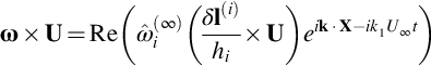
where δl(i) are displacement coordinates shown in Fig. 6.3. Since δl(1)/h1=U/U∞ we can use the relationship given by Eq. (6.2.9) to show that
where X2=const and X3=const are the stream surfaces of the mean flow. It follows that the source term in Eq. (7.1.4) is determined by the two components of the vorticity that are initially normal to the mean flow, and the streamwise component of the vorticity has no impact on the source term, even after distortion by the mean flow. The important consequence of this is that trailing tip vortices or other similar flows where the unsteady vorticity is initially aligned with the mean flow can only cause sound radiation because of nonlinear or self-induced unsteady motion.
7.2 Sound from two line vortices in free space
A simple canonical model of vortex sound [1] is given by two line vortices of equal strength Γ that are separated by the distance 2d in an otherwise stationary fluid, as shown in Fig. 7.1. The vortex pair will spin about the point halfway between them because of the induced flow at each vortex. Because there is no background flow, the motion of each vortex is caused only by its convection by the other vortex in the pair, and so each moves with a speed of U=Γ/4πd.

The location of each vortex is given as y=±y(v) where y(v)(τ)=(dcos(Ωτ), dsin(Ωτ), 0), and the angular velocity of the system is Ω=Γ/4πd2 and U=Ωd. The vorticity of each vortex is defined as
where k is a unit vector pointing out of the page in Fig. 7.1. It follows that the Lamb vector in Eq. (7.1.4) is

Note that, with the vorticity lumped into discrete vortices, the velocity field of the flow v can be replaced with the convection velocity of the vortices. Using Eq. (7.2.2) in Eq. (7.1.4) and integrating over y1 and y2 gives the sound field as

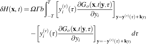
The integral is carried out over the infinite length of the two vortices because this is a two-dimensional problem. However, if we consider the sound radiation from a small linear segment of the vortices we can evaluate the far-field sound from that segment. This enables us to use the far-field approximation for the Green's function. The far-field sound from the segment of length b centered on y3 is then δH, where
We note from this result that if we were to ignore the effect of retarded time then the integrand would be zero, giving no far-field sound. However, if we expand the Green's function using a Taylor series expansion about the point ky3
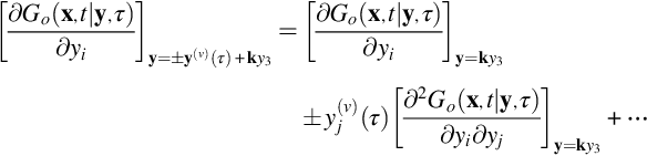
and so the integral reduces to
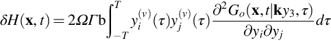
and we obtain an acoustic field that has the characteristics of a quadrupole. As we did in Section 4.4, in the acoustic far field we can shift the derivative of the free-space Green's function so that they are derivatives with respect to time, and then integrate over source time, so we obtain
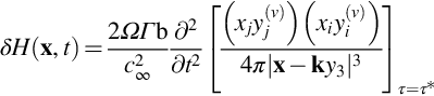
The analysis is simplified if we choose the observer location to be at x=(Ro,0,0) which gives xiyi(v)=Rodcos(Ωτ). We then obtain
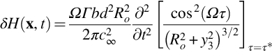
Since cos2(Ωτ)=(1+cos(2Ωτ))/2 we can simplify the integrand so that it only depends on cos(2Ωτ) because the constant term will not contribute to the acoustic field.
Then since the correct retarded time is
we obtain

We can then evaluate the far-field pressure because ∂H/∂t is approximately equal to (1/ρo)∂p/∂t in the acoustic far field. To obtain a scalable result we can define a Mach number of the vortex motion as M=Ωd/c∞, and the speed of the vortex as U=Ωd=Γ/4πd so the far-field pressure signal is given by
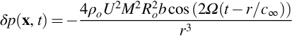
This is a canonical example of two-dimensional flow noise and as such it is valuable to investigate the important features of the result. It shows that the far-field pressure from an elemental part of the vortex scales as U2M2 which is the same as the result obtained in Chapter 4 for free turbulence. The acoustic intensity in the far field I=|p|2/(2ρoc∞) will scale as M4U4 or the eighth power of the velocity at the vortex. Eq. (7.2.6) also shows that the acoustic radiation occurs at a frequency that is twice the angular speed of the vortex, which is to be expected since the flow field replicates itself after half a revolution of the vortex pair.
Some care needs to be taken when evaluating this result for a line vortex whose span exceeds the acoustic wavelength. The result given by Eq. (7.2.6) needs to be integrated along the length of the vortex and the motion is only specified by the model given above if the vortex is of infinite length. The infinite length vortex results in a two-dimensional problem and the far-field approximations used above will no longer be valid, and the result will scale differently, but the problem can be solved exactly [2]. However, if the vortices are of finite length, and their span is acoustically compact, but their motion is well approximated by the self-induced spinning motion used above, then the far-field sound is given by the integral of Eq. (7.2.6) over y3.
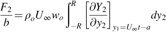
7.3 Surface forces in incompressible flow
In Chapter 4 we showed that, for acoustically compact bodies in low Mach number flows, the flow noise is dominated by dipole sources whose strength is directly proportional to the unsteady loading on the body surface. In this case the acoustic wavelength is much larger than the size of the body, and so the unsteady loading will be dominated by the incompressible part of the flow perturbations. We can therefore separate the problem into two parts, the incompressible flow that causes the unsteady load and the sound radiation from the loading on the surfaces. When this approximation is made, the acoustic far field can be evaluated from Curle's equation (4.4.7) with the source term defined by the unsteady loading caused by incompressible flow perturbations.
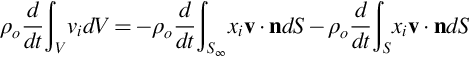
In an incompressible flow the force applied to the fluid by a stationary surface can be calculated directly from the vorticity in the flow (see Ref. [2] for a more detailed derivation of the results that follow, in which the effect of viscosity is included). To obtain this relationship consider the problem illustrated in Fig. 7.2 where fluid is bounded by a surface S∞ at a large distance from the body and the mean flow tends to a constant on this surface. Since the fluid is assumed incompressible its density will be constant and the divergence of the velocity v will be zero. The surface of the body is assumed impenetrable and so v·n on S, and we will assume that |v|2 tends to ![]() on S∞ with a difference that tends to zero as 1/rα, where α>2. This implies that there is no net flux of momentum across S∞ because in the limit that r tends to infinity (ρv·n)v=ρU∞2n1 which integrates to zero on S∞.
on S∞ with a difference that tends to zero as 1/rα, where α>2. This implies that there is no net flux of momentum across S∞ because in the limit that r tends to infinity (ρv·n)v=ρU∞2n1 which integrates to zero on S∞.

The force applied to the fluid by the body Fi can be equated to the fluid momentum and the pressure on S∞ using Eq. (2.3.3), with the assumption that there is no net flux of momentum across S∞ giving
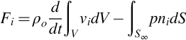
(where in this case the normal is chosen as n=−n(o) so it points into the enclosed volume). The volume integral can be changed to a surface integral by making use of the identity
and noting that the last term is zero in an incompressible fluid. Substituting this into the volume integral in Eq. (7.3.1) and using the divergence theorem results in
The boundary condition on the surface of the body requires that v·n=0, so the surface integral over S is zero and we can write Eq. (7.3.1) as
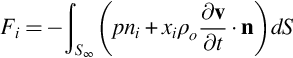
(where d/dt has been replaced by ∂/∂t inside the integral because the surface is stationary).
The right side of Eq. (7.3.2) can be related to the vorticity in the flow by making use of Kirchhoff coordinates and the form of the momentum equation given by Eq. (2.5.3). The Kirchhoff coordinates Yi are defined as equal to the potential of the flow around the body that results from an inflow on S∞ of unit amplitude in the xi direction. They have the properties that

If we take the dot product of ![]() with the momentum equation expressed in the form given by Eq. (2.5.3) and integrate over the volume of the fluid then, ignoring viscous terms for a homentropic flow, we obtain
with the momentum equation expressed in the form given by Eq. (2.5.3) and integrate over the volume of the fluid then, ignoring viscous terms for a homentropic flow, we obtain

The first volume integral on the left of this equation can be turned into a surface integral over S∞ in exactly the same way as was done for Eq. (7.3.2). Similarly the integrand of the second volume integral can be turned into a divergence because Yi is a solution to Laplace's equation. Then making use of the boundary conditions on the surface defined in Eq. (7.3.3) we find that
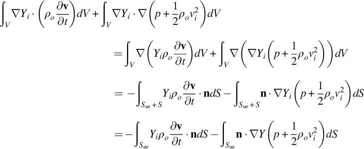
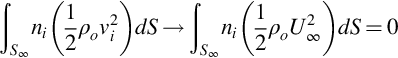
Since the surface lies at infinity we can use the limiting values given by Eq. (7.3.3) to obtain

Then since the velocity tends to its value in the uniform flow with an error proportional to 1/rα where α>2 and S∞ increases as r2 the integral of the squared velocity term becomes
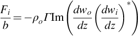
By matching terms in Eq. (7.3.2) we obtain the force applied to the fluid by the body in terms of the volume distribution of the Lamb vector ω×v as

To evaluate this integral, we need to include the vorticity throughout the fluid, including any bound vorticity such as the vorticity in the surface boundary layer and the wake behind the body. However, since the mean vorticity and mean velocity in the boundary layer next to the surface of the body will be parallel to the surface, the Lamb vector near the surface will point in the direction of the surface normal which is orthogonal to ![]() . This greatly reduces the contribution from the blade boundary layer velocity fluctuations in this calculation. However, the vorticity in the wake behind the body, that is an extension of the surface boundary layers, cannot be ignored and may play a dominant role. The other important conclusion from this result is that stationary vorticity does not contribute to the unsteady loading, so we need to only consider vorticity that is convected when evaluating Eq. (7.3.4). Also we note that the streamwise force is given by the F1 component
. This greatly reduces the contribution from the blade boundary layer velocity fluctuations in this calculation. However, the vorticity in the wake behind the body, that is an extension of the surface boundary layers, cannot be ignored and may play a dominant role. The other important conclusion from this result is that stationary vorticity does not contribute to the unsteady loading, so we need to only consider vorticity that is convected when evaluating Eq. (7.3.4). Also we note that the streamwise force is given by the F1 component ![]() . If the vorticity is convected by the potential mean flow around the body then
. If the vorticity is convected by the potential mean flow around the body then ![]() , and there will be no streamwise force. The streamwise force is therefore determined by the deviation of the vortex path from the potential flow streamlines, which results from the influence of other regions of vorticity or the image vorticity inside the body that impacts the vortex trajectory in the flow.
, and there will be no streamwise force. The streamwise force is therefore determined by the deviation of the vortex path from the potential flow streamlines, which results from the influence of other regions of vorticity or the image vorticity inside the body that impacts the vortex trajectory in the flow.
When vorticity is close to a rigid surface it will be convected by both the local mean flow (which would still exist if the vorticity was zero) and a self-induced flow that is required to meet the non-penetration boundary condition on the surface. The self-induced flow is often characterized by equivalent image vorticity that is placed inside the surface but is a potential flow outside the surface. The image vorticity can have a big impact if the path of the vortex takes it close to the stagnation point, but little impact if the vortex is relatively weak and some distance from the surface. To assess the importance of this we will consider a line vortex near a surface and estimate the velocity induced by the image vortex to be Γ/4πδ, where δ is the distance of the line vortex from the surface and Γ is its circulation. Then if Γ/4πUδ≪1 (where U is the local mean flow speed) the motion induced by the image vortex will not be important. However, this criterion cannot be met close to the stagnation point at the front of the body where the mean flow speed tends to zero. In this case the motion of the vortex will be controlled by the induced flow and the amplitude of the unsteady loading will be of order ρoΓ2/4πδ. However this will only have a small impact on the unsteady loading pulse which will have a peak amplitude of order ρoΓU∞. This leads to a criterion that requires Γ/4πU∞δ≪1, which is less restrictive than the criterion based on the local flow speed. In real flows one might expect Γ/2π~uoL, where uo is a typical gust velocity and L is the lengthscale of the turbulence. Typically, L~δ, so the importance of the self-induced motion of the vortex will depend on uo/4πU∞ which is very small in most flows of interest for which uo≪U∞. Therefore, we will not consider the impact of the image vortex on the convection speed any further, and we will assume the vortex is simply convected by the mean flow.
7.4 Aeolian tones
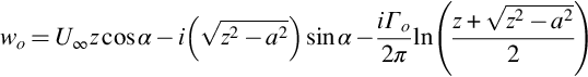
A well-known phenomenon of sound caused by flow over solid bodies is the Aeolian tone. This describes the mechanism of sound generation from the wind blowing through boat rigging and over telephone wires, or any other cylindrical body. The mechanism responsible for Aeolian tones has been studied extensively and is a classic example of vortex sound. The flow is illustrated in Fig. 7.3, which shows a stationary cylinder in a uniform flow, which sheds well-defined vortical structures into its wake. The vortical structures form a von Kármán vortex street that consists of equally spaced vortices that are convected downstream at a constant speed. At Reynolds numbers Red=U∞d/v (based on the flow speed U∞ and the cylinder diameter d) that lie in the range 40<Red<5×10⁴ it is found that well-defined vortical structures are shed periodically, and the frequency of vortex shedding f is given by a Strouhal number St=fd/U∞ of approximately 0.2. This is a weak function of Reynolds number and given by Goldstein [3] as

Flow visualization of the wakes behind cylinders have shown that the formation of the wake vortices follows a consistent process. As shown in Fig. 7.3 the vortices are initiated just behind the cylinder on either the upper or lower side of the wake.
During the period of growth, the vortex is almost static as it spins up, extracting circulation from the boundary layer on the surface of the cylinder. Once it has reached a critical circulation, it detaches from its point of initiation and is swept downstream by the flow. The initial period of acceleration is quite fast, and once it reaches the wake region it is convected with constant speed Uc. The process is then repeated for a vortex in the lower part of the wake, and it grows and separates in exactly the same way as the vortex in the upper part of the wake. The process is then repeated resulting in a time varying, periodic flow.
The periodic vortex shedding causes an unsteady lift fluctuation on the cylinder that is readily understood by using the results given in Section 7.3. In terms of Eq. (7.3.4) the unsteady lift on the cylinder will be given by

where the function Y2 is the velocity potential of a flow of unit free-stream velocity in the i=2 direction around the cylinder and is given by Eq. (2.7.27) as

The first thing we note from Eq. (7.4.1) is that, since we are assuming that the vorticity is concentrated at a point in the flow, there will be no unsteady load while the vortex is stationary during its period of growth because v=0. However, once it reaches its critical strength and starts to move then it will contribute to the unsteady load. Vortex formation occurs at a point lo>d downstream from the center of the cylinder, and so when the vortex is in motion we can approximate Y2~y2 and the trajectory is almost parallel to the y1 axis, so we can write
where u(t−tn) is the speed of the vortex after it detaches at time t=tn and is zero for t<tn. The location of the vortex in the downstream direction is given by lo+s(τ), where τ is the time since the vortex was shed and s(τ) is the distance traveled. The vertical location of the vortex is given by y2=±h/2 depending on whether it is in the upper or lower row, and the spanwise extent of the vortex is given by b. Furthermore the vortices shed in the upper row will have the opposite direction of rotation to the vortices in the lower row, so Γn=(−1)nΓ. Using this model in Eq. (7.4.1) for multiple vortices then gives

If the vortex convection speed increases linearly with time until it reaches a steady convection speed Uc and the acceleration time is half a period, then we can model u(τ) such that
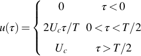
The series in Eq. (7.4.3) then represents a triangular wave with amplitude Uc, and it can be expanded into a Fourier series so that

where Ω=2π/T is the fundamental frequency of the fluctuations. We can then define a lift coefficient for the first harmonic based on the frontal area of the cylinder as

Analysis of a von Kármán vortex street [4] shows that the convection speed of the vortices in the sheet relative to a fixed body in a uniform flow is given by
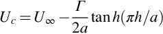
where a is the horizontal distance between vortices and is approximately a=4d for Reynolds numbers above 1000. The stability of the vortex street requires that h/a=0.281. To obtain Γ we note that the Strouhal number is directly related to the convection velocity, so St=Ucd/U∞a, and since St=0.2 the convection velocity is approximately Uc=0.8U∞. However, there is also experimental evidence that the convection velocity is higher than this and has a value of Uc=0.9U∞ [5]. Solving Eq. (7.4.6), with Uc=0.9U∞, then gives

and a lift coefficient of approximately 0.81, which is in good agreement with the measured values given by Blake [5].
The sound radiation from the unsteady loading at the fundamental frequency is readily calculated using Eqs. (7.4.4), (4.4.7), and we obtain the far-field sound as

This shows the classic dipole scaling of the far-field sound in which the acoustic intensity I=(prms)2/ρoc∞ scales as M3U∞3 and depends on the sixth power of the flow speed. Also note the directionality that has cosine dependence with a maximum in the direction of the unsteady lift.
7.5 Blade vortex interactions in incompressible flow
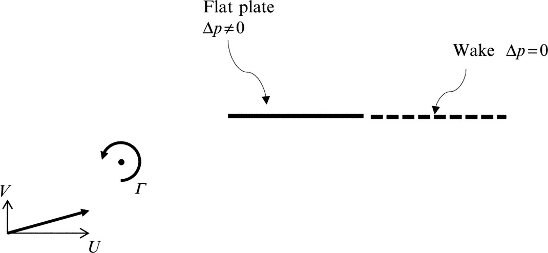
An important source of noise in aeroacoustics occurs when a blade moves past a line vortex. This is particularly relevant to helicopter noise when blade vortex interactions occur during maneuvers and cause a loud thumping sound. The source of the vortices in this case is the tips of the blades themselves. Using the formulas developed in Section 7.3 we can derive a simple incompressible flow model for the unsteady load caused by a blade vortex interaction from which we can calculate the acoustic field. More detailed analysis of this problem, which includes the effect of compressibility, will be given in Chapter 14, and here we will focus on the incompressible flow solution, using the approach given by Howe [2].
If we make the assumptions of thin airfoil theory then the blade can be modeled as a flat plate with zero thickness at zero angle of attack to the mean flow, as shown in Fig. 7.4. The vortex is convected past the plate with the mean flow U∞, and its path takes it a height h above the plate. The coordinate system is chosen to be coincident with the center of the plate and the blade chord is 2a. If we consider a line vortex with circulation Γ then we can calculate the unsteady loading per unit span of the plate on the fluid using Eq. (7.3.4). Since the direction of the vorticity vector is out of the page, and the flow is in the y1 direction the Lamb vector points in the y2 direction and the unsteady load per unit span for a vortex located at y1=U∞t, y2=h is
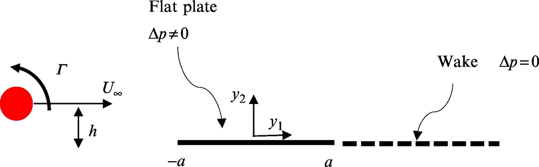

where b is the span of the blade. The Kirchhoff coordinate Y2 for a flat plate can be calculated from potential flow theory and is given by Eq. (2.7.29) with α=π/2 as
The branch cut of the square root is chosen to lie between z=±a so that there is no flow through the plate. Fig. 7.5 shows the streamlines of the flow defined by ![]() , and it is seen that the function contours around the plate, changing rapidly for locations near the leading and trailing edges. Using this in Eq. (7.5.1) then gives the unsteady loading as a function of time as
, and it is seen that the function contours around the plate, changing rapidly for locations near the leading and trailing edges. Using this in Eq. (7.5.1) then gives the unsteady loading as a function of time as

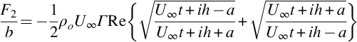
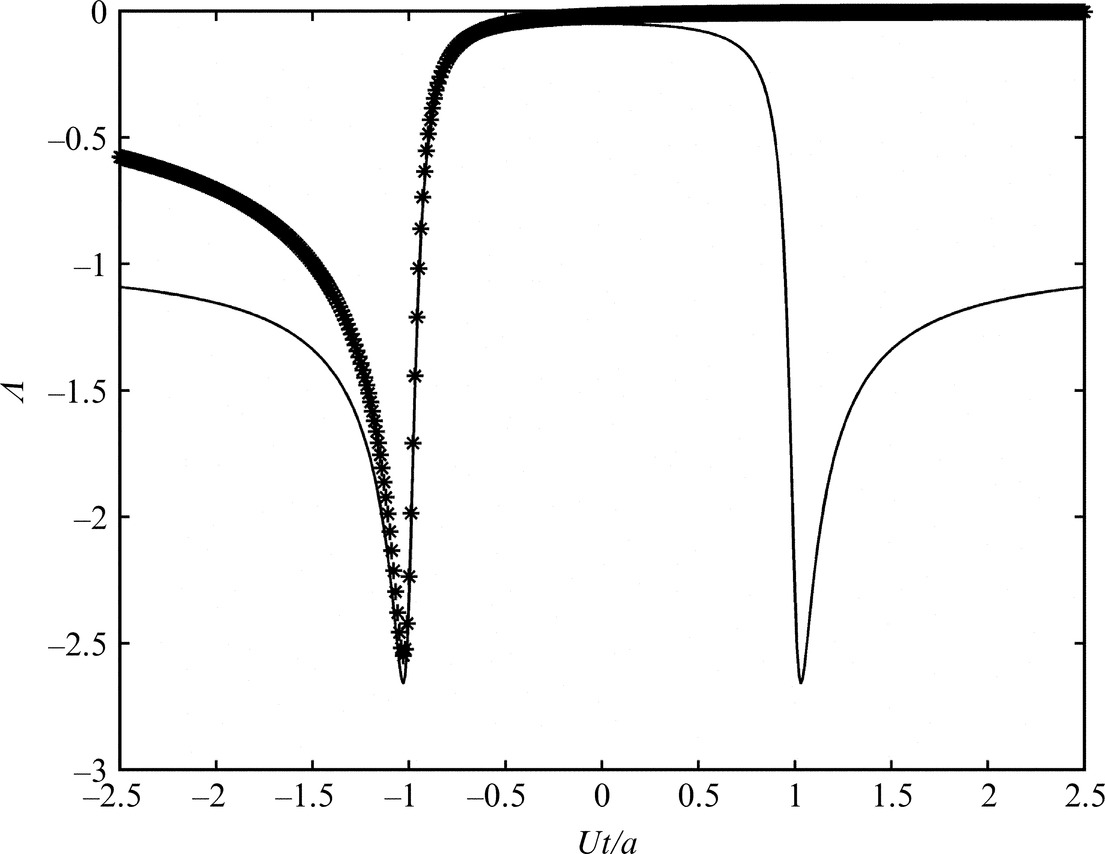
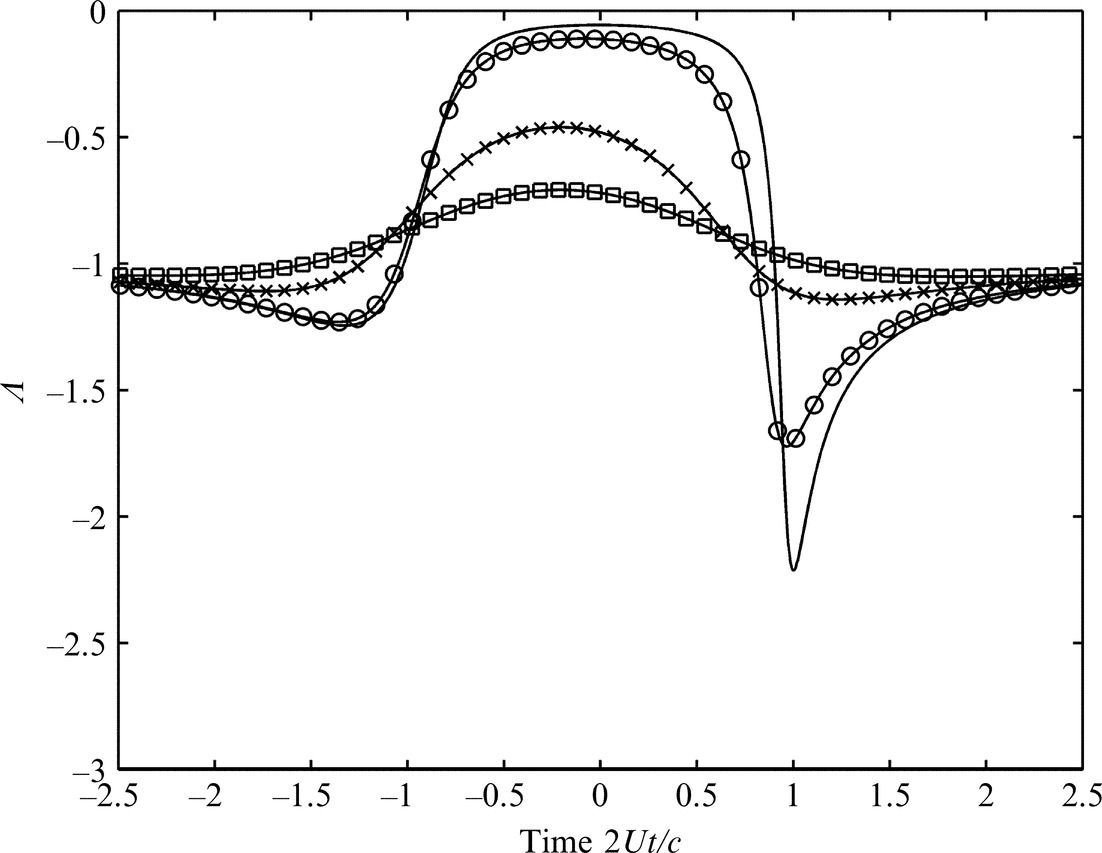
(note: this is the force applied to the fluid that tends to a constant when t=±∞ because the vortex remains in the flow). The time history of the unsteady load therefore has two contributions. The first has a peak when U∞t=−a, which corresponds to the location of the vortex when it is closest to the leading edge of the blade. The second contribution occurs when U∞t=a, which corresponds to the location of the vortex when it is closest to the trailing edge. These pulses are shown in Fig. 7.6, and their peak levels are determined by the height of the vortex above the surface, so the results for different values of h/a are shown. The closer the vortex is to the blade the sharper and larger is the unsteady loading pulse, and the leading and trailing edge pulses are of the same magnitude.

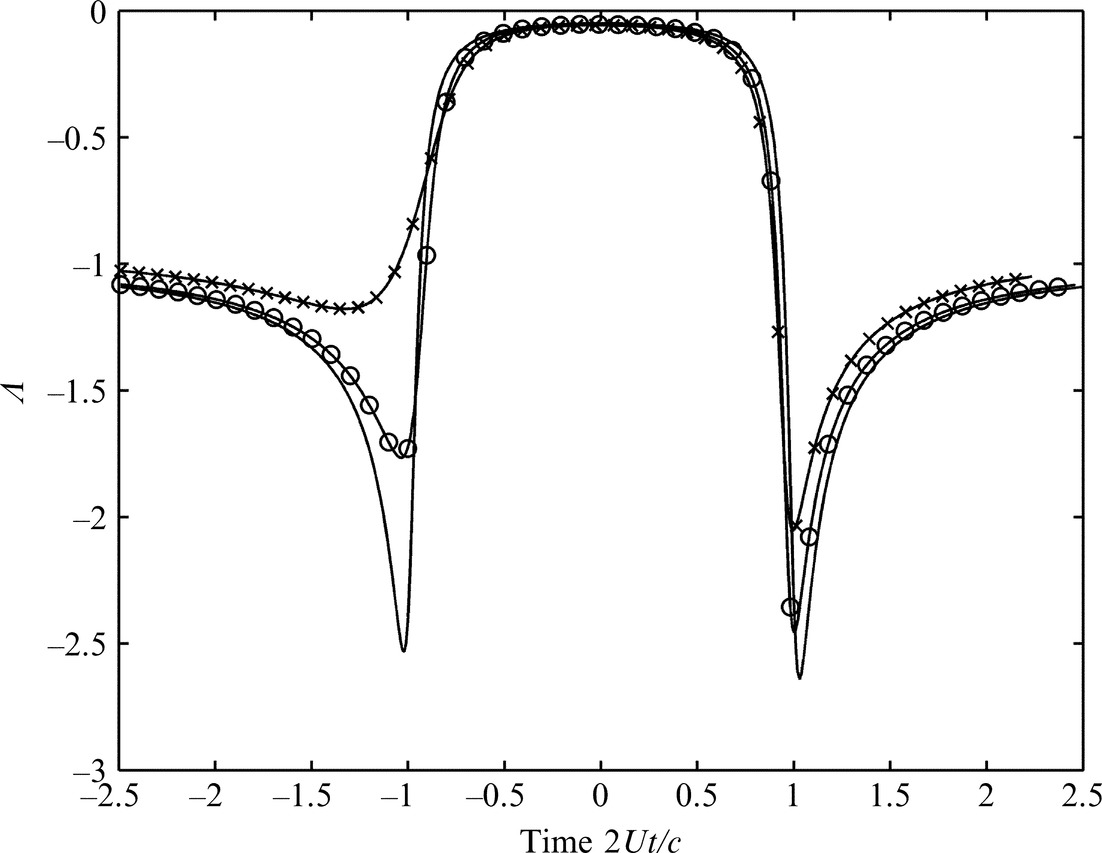
However, this model has not included the effect of vorticity in the blade wake, which is required to satisfy the Kutta condition. To fully calculate the impact of the wake vorticity we would need to solve the equations of motion to obtain the shed vorticity as a function of time. However, the impact of the wake vorticity is to eliminate the pressure jump at the trailing edge of the blade, and it was argued by Howe [2] that this reduces the trailing edge pulse. This leads to Howe's approximation which applies to the case when the vortex is close to the blade, so h≪a. It approximates the net unsteady loading by the contribution from the leading edge pulse only, and sets the trailing edge pulse to zero, so the unsteady load is given by the first term in Eq. (7.5.3) in the limit that U∞t=−a, as

A comparison between Howe's approximation and the total pulse is shown in Fig. 7.7 for a vortex that passes above the blade at a standoff distance of h/a=0.05.
To justify this approximation, we need to compare the results using Howe's approximation to the solution that would have been obtained using an exact incompressible flow calculation that includes the Kutta condition. For a harmonic gust this is given by Sears function, which was discussed in Chapter 6. The comparison is most easily carried out by considering a gust that is caused by a harmonic vortex sheet at distance h above the blade. This causes a velocity field given by
It is readily verifiable that this flow is incompressible, and the vorticity is only nonzero on the vortex sheet and has a single component in the i=3 direction given by ![]() .
.
Using this result in Eq. (7.3.4), we assume that the amplitude of the velocity fluctuations is very much less than the mean flow speed, giving the unsteady load as
Using Howe's approximation this becomes
This integral can be evaluated using tables of Fourier transforms, and it is found that
We can compare this with the high-frequency approximation to the unsteady loading calculated using Sears function using Eqs. (6.4.3), in the limit that k1a=σ≫1. In Eq. (6.4.3) the gust was defined relative to the upwash on the blade, and so the equivalence between the magnitude of the gust response given by Eqs. (6.4.3), (7.5.6) for σ≫1 requires that the upwash gust amplitude is replaced by exp(−k1h) in Eq. (7.5.6). Comparing Eqs. (6.4.3), (7.5.6) shows that they give the same gust magnitude in the limit that σ≫1. Consequently Howe's approximation correctly accounts for the effect of vortex shedding in the wake and the Kutta condition and leads to the conclusion that the unsteady loading from a blade vortex interaction is dominated by the response of the blade as the vortex passes leading edge of the blade, hence the term Leading Edge Noise which we will discuss in more detail in subsequent chapters.
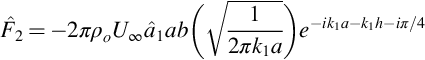
Another example that is of interest and also verifies Howe's approximation is the response of a flat plate to a step gust. In this case the incident disturbance is specified by the velocity and vorticity distribution where the gust reaches the leading edge at t=0. We assuming wo≪U∞, the unsteady loading per unit span is
At first sight this integral would appear trivial and gives the load as 2ρoU∞woR which does not vary in time. However, there is an additional contribution when the step gust passes the leading edge of the blade because Y2 has a discontinuity on y2=0 between y1=±a. The contribution from the discontinuity is given by the jump in the value of Y2 across the surface. Applying Howe's approximation to Eq. (7.5.2) gives the jump in Y2 as
where ɛ tends to zero. The response to a step gust is then given by

This can be compared to the approximate form of Kussner's function [6] for the response of a plate to a step gust, which is given by

These results are compared in Fig. 7.8 and there is good agreement when the nondimensional time is less than one.
In conclusion the response of a blade to different types of gusts including a blade vortex interaction, a harmonic upwash gust and a step gust, is well approximated using Eq. (7.3.4) and Howe's approximation, which assumes the unsteady load is defined by the pulse that occurs when the disturbance is close to the leading edge of the blade.
7.6 The effect of angle of attack and blade thickness on unsteady loads
7.6.1 The effect of angle of attack
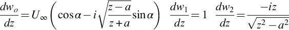
The calculation of the unsteady load produced by a two-dimensional body in an ideal potential flow can be carried out using Eq. (7.3.4) using a conformal mapping approach. This is particularly useful when considering the unsteady loading produced by airfoils at an angle of attack to the mean flow. This is not part of Sears theory since thin airfoil theory assumes that the effect of angle of attack is of second order on the unsteady loading and so is ignored. To evaluate its effect consider the unsteady loading caused by a line vortex with circulation Γ that is convected by a two-dimensional steady flow with velocity v=(U,V,0) past a flat plate airfoil as illustrated in Fig. 7.9. The vortex is defined as having its axis in the y3 direction and so, by using Eq. (7.3.4), the unsteady loading per unit span is given by

where Yi is the potential of a flow that has a speed of unit amplitude from the i direction at infinity. Since the flow around the body is incompressible and irrotational it can be specified in terms of a complex potential w(z)=ϕ+iψ, where z=y1+iy2, ϕ is the velocity potential, and ψ is the stream function of the flow. The steady flow over the surface, and the flow defining Yi can then be specified as
and the unsteady loading can be written in terms of the complex potentials as
where the * represents the complex conjugate.
To illustrate the application of this result we will consider a flat plate airfoil as shown in Fig. 7.9, where the flow is incident at an angle of attack α to the chord line. The complex potential of the flow can be obtained using conformal mapping and is given by Eq. (2.7.29) as
The circulation Γo defines the steady circulation around the airfoil, and to satisfy the Kutta condition at the blade trailing edge we require that Γo=−2πaU∞sinα (Eq. 2.7.30). We can use this result along with the complex potentials that define the flow in the y1 and y2 directions, which are
to give the derivatives needed for Eq. (7.6.3) as,
However, the results are more easily interpreted if we use Howe's approximation and limit consideration to the leading edge pulse. This also corrects for the unsteady Kutta condition at low angles of attack and so is more likely to be accurate than a direct evaluation of Eq. (7.6.3). In this approximation the complex potential is evaluated in the limit that z tends to −a so that
The two components of the unsteady load then separate out readily, and the evaluation of Eq. (7.6.3) gives
The first important feature to note about this result is that the unsteady force normal to the blade F2 is simply cosα times the unsteady force given by Eq. (7.5.4) for a vortex located at z=U∞t+ih. In addition, there is a force F1 in the direction of the blade chord, which is a suction force because it is negative. The dependence on vortex location as a function of z is identical in each case, and the direction of the force vector is given by the vector components (−2sinα, cosα, 0). For small angles of attack this corresponds to rotating the direction of the force anticlockwise through the angle 2α as shown in Fig. 7.10.

The effect of the angle of attack on the amplitude of the pulse is relatively small and causes an increase in loading of (1+3sin2α)1/2 which is minimal for small α. This result suggests that the effect of a small angle of attack on the unsteady loading is simply to rotate the direction of the load without affecting its amplitude.
However, the results given above are based on a fixed vortex displacement above the surface h, and we have not considered the effect of the rate of change of vortex position on the timescale of the pulse. If the vortex is convected by the mean flow along a streamline then its velocity is given by (dwo/dz)* as defined in Eq. (7.6.5). In the vicinity of the leading edge where the pulse reaches its largest values we can approximate z+a as equal to h, where |h| is the closest distance of the vortex to the leading edge. The velocity of the vortex will depend on (1+2a/h)1/2, and this will have only a minor impact on the vortex velocity if (2a/|h|)1/2sinα≪1. For angles of attack of less than 6 degrees this implies that we require (|h|/2a)1/2>0.1. It follows that if the vortex trajectory meets this criterion then the velocity of the vortex near the leading edge is not strongly affected by its proximity to the surface, and so the time scale of the pulse will remain the same as it was for zero angle of attack, and the leading order effect is simply the rotation of the direction of the force. However, in situations where the vortex passes closer to the leading edge than required by this limit then the vortex speed will be affected by the local flow speed, and some pulse distortion can be expected.
7.6.2 The effect of airfoil thickness
The same approach may be used to evaluate the effect of blade thickness on the unsteady loading. If we consider the Joukowski airfoil discussed in Section 2.7, then we can define the complex potential using Eqs. (2.7.32), (2.7.33). It will be assumed that the vortex is convected along a streamline, and so we need to take into account both the motion of the vortex and its location in drift coordinates.
To evaluate the streamlines of the flow and the drift coordinates around the airfoil we make use of the conformal mapping given in Table 2.1 so that
and evaluate ζ from Eq. (2.7.32) for a blade of finite thickness and no circulation, so

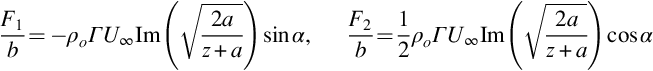
and the branch cuts are chosen, so the real part of each square root is positive. The streamlines for the flow over an airfoil with ζ1=−0.3C and C=a/2 are shown in Fig. 7.11A.
The vortex will be convected by the mean flow, and if its circulation is sufficiently small that nonlinear convection effects can be ignored then the position of the vortex at any time will be determined by the drift coordinates of the mean flow. The drift coordinate X2=ψ/U∞ is simply the stream function of the mean flow normalized on the velocity, and the surfaces of constant drift along the streamline can be evaluated from the integral of the velocity along the streamline as
where wo is given by Eq. (2.7.33) evaluated with wo=w, α=0, and Γ=0 for a blade at zero angle of attack.
The drift coordinates are shown in Fig. 7.11B and illustrate how the vortex that passes close to the airfoil will be retarded in comparison to the vortex that passes well above the airfoil. If the vortex is on the stagnation streamline then it comes to rest at the leading edge stagnation point and so is not convected over the surface unless it is ejected into the flow by a nonlinear interaction with the surface, caused by the image vortex required to match the non-penetration boundary condition. In a turbulent flow this ejection could cause the vortex to pass over either the upper or lower surface, so the net contribution from vorticity on the stagnation streamline is indeterminate.
Since the blade is symmetrical in this example, and the vortex is modeled as following a streamline, the unsteady loading caused by the passage of the vortex can be obtained from the complex velocity of the mean flow, as specified in Eq. (7.6.3). The terms required in this equation are obtained from Eq. (2.7.33) as
Using these results in Eq. (7.6.3) then gives the unsteady loading for a vortex located at a point ζ on the streamline where

and as before the branch cuts are chosen so that square roots have a positive real part.
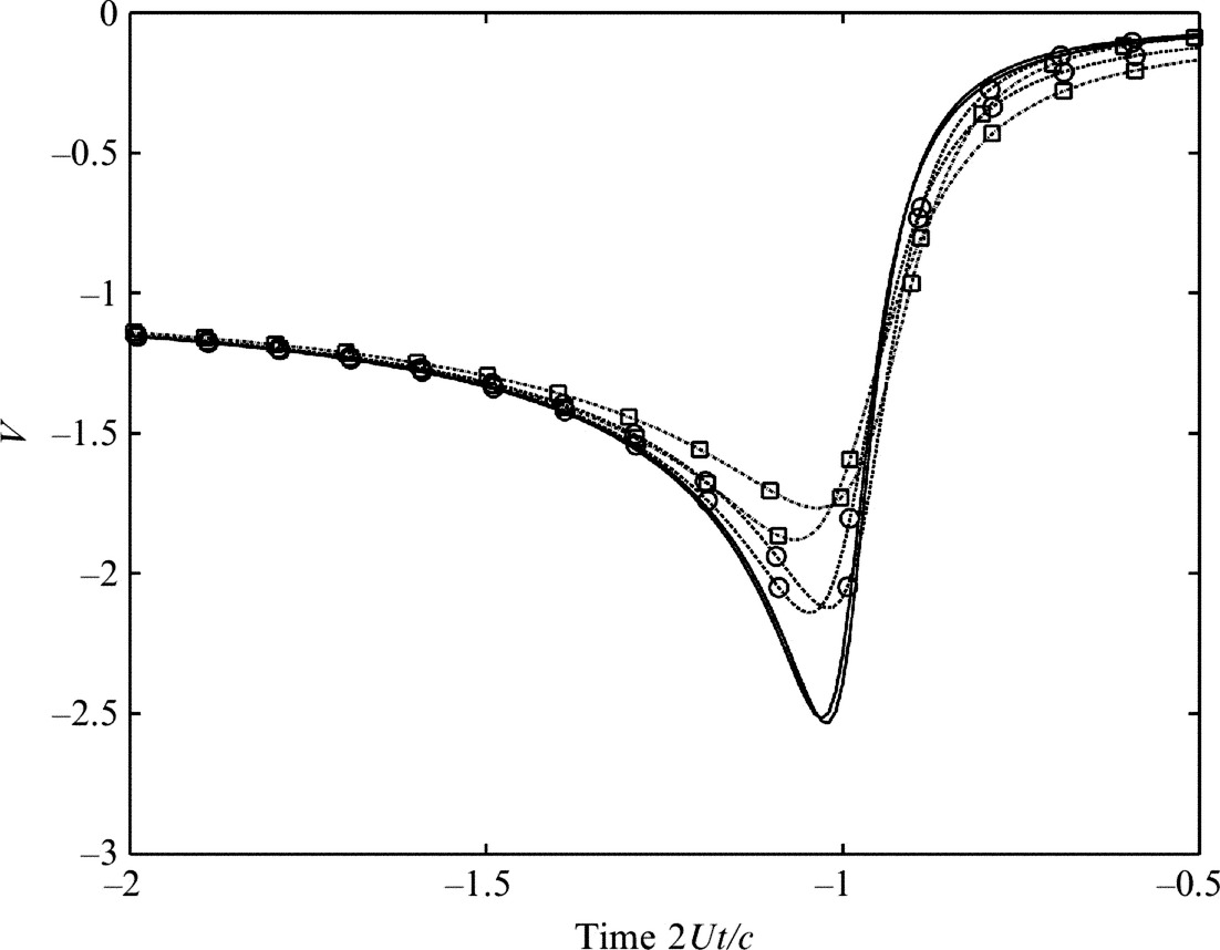
Fig. 7.12 shows the unsteady loading for a vortex passing at different distances from the blade shown in Fig. 7.11. The effect of the blade thickness on the leading edge pulse when compared to the results presented in Fig. 7.6 is significant. The sharpness of the leading edge pulse is smoothed, but the effect of thickness on the trailing edge pulse is relatively small. It is also noteworthy that when the vortex is on a streamline that is close to the airfoil the pulse is independent of the displacement of the vortex, indicating that for thick airfoils the proximity of the vortex to the stagnation streamline is unimportant.
This example is for a very thick airfoil, and the effects of thickness for thin airfoils are better shown by considering a vortex at a fixed starting point being convected past an airfoil of different thicknesses, as shown in Fig. 7.13. The three cases shown are for an airfoil with thickness to chord ratios of 1.2%, 12%, and 30%, respectively. As before the effect of thickness is to reduce the leading edge pulse and has a much smaller effect on the trailing edge pulse. We also note that the effect of thickness is nonlinear and that for the thick blade (as in Fig. 7.12) the leading edge pulse is significantly smoothed.
Clearly the effect of thickness on the unsteady loading is to smooth out the leading edge pulse that occurs as the vortex interacts with the leading edge of the blade. It has less effect on the trailing edge pulse, but that is inconsequential because in these examples the Kutta condition has not been introduced. The smoothing of the leading edge pulse implies that the high-frequency content of the blade response function will be reduced by thickness effects. The effect of the blade thickness appears as if the vortex passes further from the blade than it would if the blade was a flat plate. This scales on the blade thickness to chord ratio, and Fig. 7.14 shows a comparison between the unsteady loading from airfoils of thicknesses of 1.2%, 6%, and 12% with a vortex initiated at the same point upstream and is compared to the unsteady loading calculated using a flat plate approximation with the vortex displacement increased by half the thickness of the blade. The curves are remarkably close, and this provides a first-order scaling on the effect of blade thickness on the unsteady loading.
We can also estimate the effect of blade thickness on the blade response function in the frequency domain by modifying Eq. (7.5.6) so that the displacement of the vortex h is increased by half the thickness of the blade. This will reduce the high-frequency content of the blade response function by a factor of exp(−ωtmax/2U∞), where tmax is the thickness of the blade, and so the high-frequency content of the blade response function is reduced by an exponential factor that depends on the blade thickness. However, it should be noted that this analysis is for incompressible flow and assumes that the blade and wake respond instantaneously to an incoming disturbance. We will show in Chapter 14 that this approximation is only valid when the blade chord is less than one-quarter of the acoustic wavelength. The discussion outlined above shows that blade thickness is only important when ωtmax/U∞>1. The incompressibility criteria requires that ω<πco/2c and so for the effect of blade thickness to be modeled by an incompressible model we require πtmax/2cM>1 or that the flow Mach number is less than 0.19 for a 12% thick blade. In most aeroacoustic applications the blade Mach number exceeds this criterion and so compressibility effects have to be considered.