
Turbulence and stochastic processes
Abstract
This chapter discusses the stochastic nature of turbulence and the sound fields produced by the interaction of a generic surface with a turbulent flow. The generation of turbulence at the largest scales, the energy cascade and dissipation are described, and the Reynolds averaged Navier Stokes (RANS) equations are introduced including the concept of a turbulence model. Computational methods based on these concepts are discussed, outlining a range of methods for computing turbulent flows including RANS, unsteady Reynolds averaged Navier Stokes, large eddy simulation, and direct navier stokes. The chapter also introduces the necessary descriptors of turbulence for aeroacoustic analysis, such as correlation functions and integral scales, frequency spectra, cross spectra and cross correlations, coherence and phase, and wavenumber spectra in multiple dimensions in homogeneous and inhomogeneous flows.
Keywords
Turbulence; Turbulence models; Spectral analysis of stochastic processes; Frequency and wavenumber spectra; Correlations and lengthscales
This chapter discusses the stochastic nature of turbulence and the sound field produced by the interaction of a generic surface with a turbulent flow. The generation of turbulence at the largest scales, the energy cascade and dissipation are described, and the Reynolds averaged Navier Stokes (RANS) equations are introduced including the concept of a turbulence model. Computational methods based on these concepts are discussed. The chapter also introduces the necessary descriptors of turbulence for aeroacoustic analysis such as correlation functions integral scales frequency spectra, cross spectra cross correlations coherence phase wavenumber spectra in multiple dimensions in homogeneous inhomogeneous flows.
8.1 The nature of turbulence
It is tempting to think of sound as an entirely deterministic phenomenon. The representation of sound fields as harmonic waves in space and time engenders an image of acoustic fields formed by the ordered propagation of entirely predictable periodic variations in density and pressure. There are many applications in aeroacoustics where this is the case, for example: the sound field generated by the thickness noise of a rotating propeller or the tones generated by a set of rotor blades as they cut through a nonuniform flow field. In many cases, however, sources of sound result from the unsteadiness of a turbulent flow and they, and the sound fields they produce, are stochastic.
Turbulence is chaotic, vortical motion found in the rotational regions of flows, such as boundary layers, wakes, and jets, where viscosity has influenced the motion. Turbulence in low Mach number flows is usually considered incompressible. Even though the mean motion may be compressible, the turbulent fluctuations in velocity are rarely more than 10–20% of the mean and thus do not have a significant Mach number.
Turbulence is initiated and maintained by viscous instability and characterized by eddying motions over a large and continuous range of scales. Sound produced by the action of turbulent flow therefore tends to be broadband, with energy over a continuous distribution of frequencies. On the largest scales the turbulent eddies, often also known as coherent structures, are formed by the instability and roll up of shear-layers associated with the large scale geometry of the flow, such as the von Kármán vortex street formed behind a circular cylinder (see Section 7.4). The scale of these largest structures L is comparable to the overall dimension of the flow (e.g., the wake thickness), and the scale of their velocity fluctuations, u, varies directly with the overall velocity scale of the flow U.
The shearing motions associated with these largest structures are themselves unstable, however, and so they break down into smaller structures that are themselves subject to instability. This process continues until the structures formed are small enough to be directly slowed by the molecular viscosity of the fluid. Such a structure with a size η and velocity uη experiences a viscous force that scales on μuη/η (from Newton's Law of Viscosity) multiplied by the eddy surface area that varies as η2. It experiences a loss of momentum at a rate equal to its mass times the rate of change of its velocity, which will scale on ![]() , where we have calculated the timescale for the deceleration τη as η/uη. Given that the viscous force and rate of change of momentum must be in balance, we expect that
, where we have calculated the timescale for the deceleration τη as η/uη. Given that the viscous force and rate of change of momentum must be in balance, we expect that
and thus,
where ν the kinematic viscosity ![]() . We see that the Reynolds number of the smallest scales in turbulence is of order 1. The scales η,uη,andτη are referred to as the Kolmogorov microscales after the great 20th century Russian mathematician Andrey Kolmogorov. These are most commonly expressed in terms of the rate of viscous dissipation of kinetic energy per unit mass
. We see that the Reynolds number of the smallest scales in turbulence is of order 1. The scales η,uη,andτη are referred to as the Kolmogorov microscales after the great 20th century Russian mathematician Andrey Kolmogorov. These are most commonly expressed in terms of the rate of viscous dissipation of kinetic energy per unit mass ![]() . Since
. Since ![]() we obtain
we obtain
The flow of energy from large to small scales is referred to as the “energy cascade.” Kinetic energy enters the cascade at the largest scales, at a rate that is determined by the largest motions based on the time scale L/U, i.e., at a rate, per unit mass, that scales with ![]() . All this energy must be dissipated by viscosity at the smallest scales and so, counter-intuitively, this rate
. All this energy must be dissipated by viscosity at the smallest scales and so, counter-intuitively, this rate ![]() is independent of viscosity. The ratio of the largest to smallest scales in the cascade is
is independent of viscosity. The ratio of the largest to smallest scales in the cascade is

where we have denoted the overall Reynolds number of the flow UL/ν as Re. We see, therefore, that the statement that turbulence is associated with a large range of scales is synonymous with the statement that turbulence is a high Reynolds number phenomenon. The ratio of largest to smallest velocity and time scales in the energy cascade is similarly shown to vary as Re1/4 and Re1/2 respectively.
Kolmogorov hypothesized that at sufficiently high Reynolds numbers, the smallest eddies in a turbulent flow depend only on viscosity and dissipation rate and thus are isotropic and universal between different flows. This is often referred to as the dissipation range. He also hypothesized universality in the mid-range scales, much larger than η but much smaller than L, which should therefore be determined by the rate of energy flow through the cascade, which is equal to ɛ. This is referred to as the inertial subrange. The validity of Kolmogorov's hypotheses, and the extent to which turbulent flows exhibit a universal character, remain open questions in turbulence research.
Turbulence is a stochastic phenomenon. While it is completely described by the governing equations of fluid dynamics, the instantaneous details of flow are sensitive to its history and boundary conditions in such a complex and chaotic way that deterministic predictions are simply not possible. Fortunately, the instantaneous details are rarely important since, as engineers, we care about typical behavior. We wish to know the average behavior of the turbulence, and of the sound field with which it is associated.
8.2 Averaging and the expected value
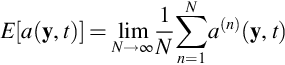
In many aeroacoustic and fluid dynamic situations we find it helpful to take the mean value. For example consider an instantaneous acoustic or fluid dynamic variable, or a combination of variables, a(y,t). We can, and often do, get the mean value of a by averaging with respect to time

where we assume an averaging time 2T long enough compared to the flow processes that the result is independent of when the averaging period occurs or how long it is. Time averaging is intuitively simple but not appropriate when the typical behavior is a function of time itself, i.e., when the flow is not time stationary.
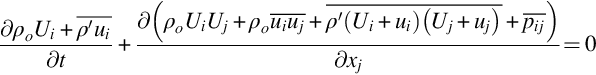
To understand this, consider the situation illustrated in Fig. 8.1 where an airfoil cuts through a turbulent wake. As this occurs, the airfoil encounters turbulence that produces an unsteady lift fluctuation and a burst of sound. The sound, the pressure fluctuations experienced on the airfoil and the eddy structures it encounters clearly will have typical characteristics, but these characteristics will depend on the position of the airfoil relative to the wake, which is itself a function of time.

To handle this kind of situation we use the more general concept of the expected value. This is the mean of the value of a stochastic variable taken over many repeated realizations of the same flow. In each realization we imagine running the flow under conditions identical in all respects, except for the stochastic behavior. Thus we can imagine obtaining multiple independent samples of our flow quantity a at the same defined position and time; e.g., for the same position of the airfoil relative to the wake. These independent samples can now be averaged to obtain a mean that remains dependent on time.
where a(n)(y,t) is the nth sample of a and N is the total number of samples taken.
As already noted we apply averaging to many variables and combinations of variables. As we will see below, averaging of products of fluctuating velocity components at the same position and time, at different positions and times, of pressure fluctuations and of the Fourier transforms of these variables appear frequently in the analysis and results of aeroacoustic problems. When the terms “average” or “mean” are used, they will refer to the expected value, unless otherwise stated. In general we will denote averaged values using an overbar, e.g., ![]() , unless a custom symbol has already been defined, such as in the case of mean velocity component Ui, or mean density ρo.
, unless a custom symbol has already been defined, such as in the case of mean velocity component Ui, or mean density ρo.
The particular types of statistical measures of turbulence that are most often required for aeroacoustic predictions become clear when the mechanisms of sound production are considered. Returning once more to the situation shown in Fig. 8.1, according to Curle's equation (4.3.9) for an impermeable stationary surface, the instantaneous acoustic pressure ![]() depends on the time and area integral of the pressure over the airfoil surface, and a volume integral of quadrupole sources that is of second order. So, the first order approximation to the sound field is given by
depends on the time and area integral of the pressure over the airfoil surface, and a volume integral of quadrupole sources that is of second order. So, the first order approximation to the sound field is given by
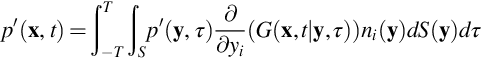
(note that the mean pressure produces no sound in this case, and viscous effects have been ignored so we can replace pij with p′ in the integrand where p′=p−p∞). To characterize the typical character of the sound field, we typically measure in the mean square acoustic pressure ![]() , for example, which is
, for example, which is
where we have used ∂/∂n to represent the gradient in the direction normal to the surface. The expected value operator ends up containing only the multiplication of the pressures since pressure is the only stochastic variable on the right hand side. The sound is therefore a function of the correlation (i.e., the average of the product) of the pressure fluctuation at y and τ, and that at y′ and τ′.
The important general point here is that average measures of the sound field will in general be functions of the two-point space-time correlations of the turbulent flow variables, and that simple averaging of a flow variable at a fixed position does not give all the information required to calculate the far field sound.
8.3 Averaging of the governing equations and computational approaches
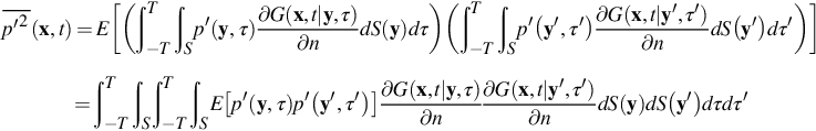
Averaging plays a key role in how we approach the numerical solution to turbulent flow problems. At low Mach number a turbulent flow is, in principle, prescribed by the continuity and momentum equations
Numerical solution to these equations for turbulent flow is possible only in very simple situations and at Reynolds numbers that are low compared to most applications. These direct Navier Stokes (DNS) solutions are primarily useful for scientific research into the fundamental physics of a flow. Engineering solutions are not possible by this method because of the inherently large range of scales present in turbulent flows at practical conditions. At an overall Reynolds number Re of one million (which is typical as it applies to a blade of chord 20 cm in a flow of 75 m/s in air), the analysis of Section 8.1 tells us that we will need to resolve a range of length scales of about 30,000:1 (Re3/4) and a range of timescales of about 1000:1 (Re1/2). Numbers like these imply vast computational memory and speed requirements.
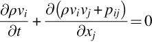
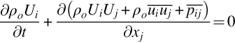
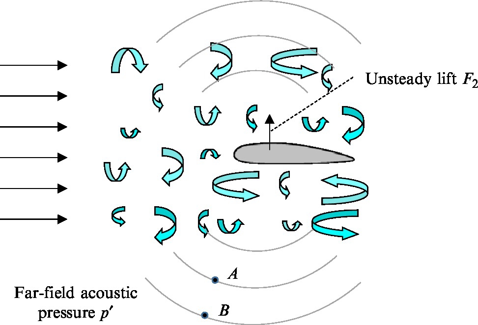
To compute turbulent flows at practical conditions and Reynolds numbers it is thus necessary to average the continuity and momentum equations. Splitting the dependent flow variables ρ, vi, and pij into their expected values and fluctuations about the mean, and taking the expected value of Eqs. (2.2.6), (2.3.9) we get, in turn

Note that the ρ′ and p′ here denote fluctuations about the mean (expected) value, rather than changes from ambient conditions. At low Mach number, terms multiplied by ρ′ can be neglected since ρ′≪ρo, and so we obtain

and
We see that averaging of continuity equation merely returns the same expression in terms of the mean flow variables and, since the averaging process represents an expected value, the mean flow quantities can vary with time and so the time derivatives are not zero. Averaging of the momentum equation also returns a similar expression in terms of the mean variables, but with the additional terms ![]() involving the velocity fluctuations. These terms (or, strictly speaking their negatives) are referred to as the Reynolds or turbulent stresses, since they appear in the equation in the same way as the mean compressive stress tensor
involving the velocity fluctuations. These terms (or, strictly speaking their negatives) are referred to as the Reynolds or turbulent stresses, since they appear in the equation in the same way as the mean compressive stress tensor ![]() .
.
When attempting to solve Eqs. (8.3.1), (8.3.2) we can specify the mean compressive stress tensor ![]() from the sum of the mean pressure and the mean viscous stresses, which can be inferred from the mean velocity gradients and the viscosity. Also we can relate the pressure and density through the energy relations described in Chapter 2 (or for incompressible flows the density may be assumed constant). In the absence of the turbulent stresses there would then be four equations with four unknowns p, U1, U2, and U3, and a solution is possible. However, when the turbulent stresses are included there is an additional set of six unknown terms,
from the sum of the mean pressure and the mean viscous stresses, which can be inferred from the mean velocity gradients and the viscosity. Also we can relate the pressure and density through the energy relations described in Chapter 2 (or for incompressible flows the density may be assumed constant). In the absence of the turbulent stresses there would then be four equations with four unknowns p, U1, U2, and U3, and a solution is possible. However, when the turbulent stresses are included there is an additional set of six unknown terms,
and thus Eqs. (8.3.1), (8.3.2) do not form a closed set. Solving them requires that we introduce empirical expressions to relate the Reynolds stresses back to the mean flow variables. These relations are referred to as a “turbulence model.” The first and most straightforward turbulence modeling concept is the Boussinesq eddy viscosity μt, remarkably proposed in 1877 [1]. Boussinesq's hypothesis is that the turbulent stresses are related to the mean velocity gradients in almost the same way that the viscous stresses are related to the complete velocity gradients. That is, by near analogy with Eq. (2.3.11) (for incompressible flow), we write

where ![]() is the turbulence kinetic energy. The eddy viscosity is considered a property of the flow, rather than the fluid, and thus is a variable that must be modeled. One classic model is the “k-epsilon” model [2] for which μt is taken to be proportional to the mean scales L and U so
is the turbulence kinetic energy. The eddy viscosity is considered a property of the flow, rather than the fluid, and thus is a variable that must be modeled. One classic model is the “k-epsilon” model [2] for which μt is taken to be proportional to the mean scales L and U so ![]() and since ɛ scales as U3/L and κe scales as U2 it follows that L/U scales as κe/ɛ and μt scales as ρoκe2/ɛ. The turbulence kinetic energy κe and dissipation rate ɛ are obtained from empirical differential equations designed to model the factors controlling the changes to a patch of turbulence as it is convected along by the mean flow. Much experimental, theoretical, and computational effort has gone into identifying and refining turbulence models, and there are many to choose from. All such models are, however, ultimately limited in application and accuracy since the models are not themselves solutions to the equations of motion.
and since ɛ scales as U3/L and κe scales as U2 it follows that L/U scales as κe/ɛ and μt scales as ρoκe2/ɛ. The turbulence kinetic energy κe and dissipation rate ɛ are obtained from empirical differential equations designed to model the factors controlling the changes to a patch of turbulence as it is convected along by the mean flow. Much experimental, theoretical, and computational effort has gone into identifying and refining turbulence models, and there are many to choose from. All such models are, however, ultimately limited in application and accuracy since the models are not themselves solutions to the equations of motion.
In 1895 Osborne Reynolds [3] derived (in incompressible form) the time averaged version of Eqs. (8.3.1), (8.3.2),

which are therefore referred to as the Reynolds averaged Navier Stokes (RANS) equations. Computational approaches that solve these equations for steady boundary conditions are referred to as RANS calculations. When the boundary conditions are unsteady (e.g., for the turbulent flow produced by an oscillating airfoil), Eq. (8.3.2) must be solved and the calculation is described as URANS. RANS and URANS calculations are feasible and regularly conducted for complete engineering configurations at full-scale conditions. Indeed, a number of commercial packages are available that perform such computations. The drawback of these methods is that a generic turbulence model is being asked to represent all the scales of the turbulence, including the largest scales that are expected to be characteristic of the specific flow conditions and geometry. The accuracy and reliability of such predictions can often be a concern. A further drawback from the aeroacoustic perspective is that the turbulence quantities computed as part of the solution are generally single-point statistics of velocity like the Reynolds stresses, κe, and ɛ, well short of the two-point quantities of velocity and pressure that are needed to completely define an acoustic source. Additional sweeping modeling assumptions are therefore normally needed to extrapolate RANS and URANS results to obtain the acoustic sources.
Time varying unsteady flows are more accurately computed using large eddy simulation (LES). Here the equations of motion, (2.2.6) and (2.3.9), are filtered to remove turbulence scales too small to be resolved by the computational grid or time step. Since the filtering is just another type of averaging, the result is equations that appear identical to Eqs. (8.3.1), (8.3.2) but where the averaged variables ρo,Ui and ![]() now include the resolved turbulent fluctuations, and where the term
now include the resolved turbulent fluctuations, and where the term ![]() represents the unknown correlations between the small scale unresolved fluctuations. A turbulence model is required for these “subgrid” stresses. The LES approach was proposed by Smagorinsky [4] who also introduced the first subgrid turbulence model, which is an extension of Boussinesq's eddy viscosity hypothesis. More sophisticated modeling approaches have since been proposed including the “dynamic model” of Germano et al. [5] in which the parameters of the model are adjusted to match the local characteristics of the resolved turbulence. LES turbulence models are expected to be more generally applicable because the larger configuration-specific turbulence scales are computed directly. The model therefore only needs to account for the small scale turbulence that is hopefully more universal in character.
represents the unknown correlations between the small scale unresolved fluctuations. A turbulence model is required for these “subgrid” stresses. The LES approach was proposed by Smagorinsky [4] who also introduced the first subgrid turbulence model, which is an extension of Boussinesq's eddy viscosity hypothesis. More sophisticated modeling approaches have since been proposed including the “dynamic model” of Germano et al. [5] in which the parameters of the model are adjusted to match the local characteristics of the resolved turbulence. LES turbulence models are expected to be more generally applicable because the larger configuration-specific turbulence scales are computed directly. The model therefore only needs to account for the small scale turbulence that is hopefully more universal in character.
The grid resolution, and thus filter size, is an important factor in performing an LES calculation. Choosing a coarse filter and grid means a faster, smaller calculation but one that places greater reliance on the accuracy of the empirical turbulence model. Choosing a sufficiently fine filter can result in calculations that approach the fidelity of DNS. The need for both computational efficiency and accuracy has resulted in the development of hybrid RANS/URANS/LES methods where computational effort can be concentrated in those regions where it is most needed.
Better resolved LES calculations can be particularly useful for aeroacoustics because some fraction of the pressure and velocity correlations that form the acoustic source terms can be computed directly from the resolved scales. This fraction obviously increases as the resolution and expense of the calculation are increased. Integration of these sources over a surface bounding the flow and using a Ffowcs Williams Hawkings surface, can then be used to determine the sound heard by an observer in the far field, within the limitations discussed in Chapter 5.
Note that in principle, the origin and propagation of sound waves can be directly computed as part of any unsteady compressible turbulent flow simulation. However, this is rarely done for low Mach number flows because of the computational challenges posed by the large disparity in the scales and fluctuation levels of sound waves and of the turbulence producing them.
8.4 Descriptions of turbulence for aeroacoustic analysis
8.4.1 Time correlations and frequency spectra of a single variable
Consider the situation shown in Fig. 8.2 where noise is being radiated by the continuous passage of turbulence over the leading edge of an airfoil. Both, the time variations of the flow properties used to describe the turbulent source (whether they be velocity or pressure) and the sound waves that are heard by a far field observer are stochastic and time stationary. It is important that we have a quantitative measure of the typical frequency content of these signals because we need to assess the impact of the sound on a human listener, and because we are interested in separating out the contributions of different turbulence scales to the acoustic source. In Chapter 3 we introduced the Fourier transform as a way to extract the frequency components of a specific waveform. Applied to a generic flow or acoustic quantity a(t) that varies with time and has zero mean, this definition is
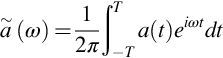
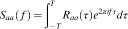
The Fourier transform ![]() is not by itself a very useful measure since, just like a(t), it will vary stochastically. The appropriate average measure of the frequency content is given by the autospectral density of a (often referred to as the autospectrum, the power spectrum, or just the spectrum) defined as
is not by itself a very useful measure since, just like a(t), it will vary stochastically. The appropriate average measure of the frequency content is given by the autospectral density of a (often referred to as the autospectrum, the power spectrum, or just the spectrum) defined as

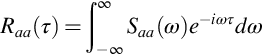
where Raa(τ) is the time delay autocorrelation function, defined as
As can be seen from this expression Raa(τ) is the average of the signal multiplied by itself at a later time. For a time stationary signal the expected value of a(t)a(t+τ) will not depend on t. The inverse Fourier transform relates the spectrum back to Raa(τ).
The definition (8.4.3) tells us that the autocorrelation function is even, i.e., it is symmetric about ![]() , because
, because
This means that the spectrum is a real and even function of frequency because Eq. (8.4.2) can be expanded as
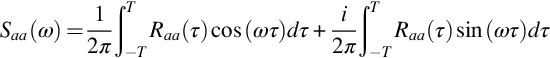
The imaginary term is zero because Raa(τ) is even and sin(ωτ) is an odd function. It also follows that Saa(ω) is an even function of frequency because cos(ωτ) is an even function of frequency.
To illustrate why the concepts of the spectrum and correlation are useful physically, consider the example shown in Fig. 8.3. Fig. 8.3A shows part of a velocity signal u1(t) measured in boundary layer turbulence near a wall where the mean flow velocity is close to 20 m/s. The signal appears quite random but, as we will see, does have a definite statistical character that reveals important information about the boundary layer turbulence. In Fig. 8.3B the time delay correlation of this signal is shown. The expected value required in Eq. (8.4.3) was obtained by calculating the product ![]() for every time instant at which the signal was measured (about 400,000 times in this particular case) and then taking the mean value of those numbers.
for every time instant at which the signal was measured (about 400,000 times in this particular case) and then taking the mean value of those numbers.

The correlation function measures how similar the signal is to its time shifted copy. At zero time delay the signals are a perfect match and the correlation has its maximum value equal, by definition, to the velocity variance ![]() (i.e., its mean square). For nonzero time delay, the correlation decays as the time shifted signal copy becomes less and less similar to the original, reaching 8% of
(i.e., its mean square). For nonzero time delay, the correlation decays as the time shifted signal copy becomes less and less similar to the original, reaching 8% of ![]() at about 0.02 s. The overall width of the correlation peak is a measure of the time scale of the largest turbulence and, indeed, the larger scales in the time signal of Fig. 8.3A do appear to be about 0.02 s. To precisely quantify this we introduce the concept of the integral timescale
at about 0.02 s. The overall width of the correlation peak is a measure of the time scale of the largest turbulence and, indeed, the larger scales in the time signal of Fig. 8.3A do appear to be about 0.02 s. To precisely quantify this we introduce the concept of the integral timescale ![]() , defined as
, defined as
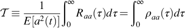
We also use this opportunity to introduce the correlation coefficient function ρaa, which is just Raa normalized on the variance, so that ![]() . In this example
. In this example ![]() integrates to a time scale of 0.0064 s. The integral time scale is usually about one third of the overall half-width of the correlation peak. If we assume that all the turbulence is traveling with a mean speed of 20 m/s then this timescale can be used to estimate the streamwise lengthscale of the flow (0.0064×20=0.128 m). In general, this type of time-to-space conversion is referred to as Taylor's frozen flow hypothesis. While it is commonly used, and probably reasonably accurate in this example, it is important to remember that it unrealistically treats the turbulence as though it didn't have velocities itself. It can therefore be misleading, particularly in flows where the turbulent velocity fluctuations are significant compared to the mean velocity.
integrates to a time scale of 0.0064 s. The integral time scale is usually about one third of the overall half-width of the correlation peak. If we assume that all the turbulence is traveling with a mean speed of 20 m/s then this timescale can be used to estimate the streamwise lengthscale of the flow (0.0064×20=0.128 m). In general, this type of time-to-space conversion is referred to as Taylor's frozen flow hypothesis. While it is commonly used, and probably reasonably accurate in this example, it is important to remember that it unrealistically treats the turbulence as though it didn't have velocities itself. It can therefore be misleading, particularly in flows where the turbulent velocity fluctuations are significant compared to the mean velocity.
It is clear that the correlation function also has information about smaller turbulence scales. For example, its initial rate of decay will reflect how much of the mean square velocity fluctuation is due to the smallest turbulence. Taking the Fourier transform to obtain the spectrum reveals this information in a more explicit way. Fig. 8.3C shows the spectrum of the velocity signal ![]() calculated according to Eq. (8.4.2). Both axes of the spectrum have been plotted on logarithmic scales to more clearly reveal the behavior in different frequency ranges. We see that the overall form of the spectrum is broken into three parts. At low frequencies, where it represents the largest motions of the boundary layer, the spectrum curves downward from a plateau. The level of this plateau is characterized by the zero frequency value of the spectrum (indicated by the horizontal line in Fig. 8.3C) which, in this case gives
calculated according to Eq. (8.4.2). Both axes of the spectrum have been plotted on logarithmic scales to more clearly reveal the behavior in different frequency ranges. We see that the overall form of the spectrum is broken into three parts. At low frequencies, where it represents the largest motions of the boundary layer, the spectrum curves downward from a plateau. The level of this plateau is characterized by the zero frequency value of the spectrum (indicated by the horizontal line in Fig. 8.3C) which, in this case gives ![]() . Looking at Eq. (8.4.2) for zero frequency, we see that this value corresponds to the integral time scale, scaled as
. Looking at Eq. (8.4.2) for zero frequency, we see that this value corresponds to the integral time scale, scaled as ![]() or, in general
or, in general ![]() . In the mid-frequency range we see that our example velocity spectrum becomes almost straight with a slope on the log-log scale of close to −5/3. As will be discussed in Chapter 9, this is indicative of an inertial subrange behavior in the mid-range scales of the boundary layer turbulence, as hypothesized by Kolmogorov. At the highest frequencies, which are assumed to be generated by the smallest eddies, the spectrum curves downward away from the −5/3rds slope as a result of the dissipation of these eddies by viscous action.
. In the mid-frequency range we see that our example velocity spectrum becomes almost straight with a slope on the log-log scale of close to −5/3. As will be discussed in Chapter 9, this is indicative of an inertial subrange behavior in the mid-range scales of the boundary layer turbulence, as hypothesized by Kolmogorov. At the highest frequencies, which are assumed to be generated by the smallest eddies, the spectrum curves downward away from the −5/3rds slope as a result of the dissipation of these eddies by viscous action.
In general, the spectrum of a time history a(t) can be physically interpreted as revealing the contributions to the mean square fluctuation ![]() at each frequency. This can be demonstrated very simply using the inverse transform relationship, Eq. (8.4.4) which, for zero time delay τ becomes
at each frequency. This can be demonstrated very simply using the inverse transform relationship, Eq. (8.4.4) which, for zero time delay τ becomes

This is known as Parseval's theorem which states that the “power” in the time and frequency domains is the same, and that the spectrum divides up that power by frequency. (Note that the term “power” is loosely used in spectral analysis to refer to the mean square.) It is in this sense that Saa(ω) is a spectral density function. We also see that the units of Saa(ω) will be the units of ![]() per radian-per-second.
per radian-per-second.
One simple but critical detail here is that the mathematical definition of the spectral density includes both positive and negative frequencies. In the present context of one-dimensional spectra these mean the same thing. However, note from Eq. (8.4.6) that the energy is spread over both the positive and negative domains. We call the spectrum double sided and this is the norm for mathematical analysis. However, in many situations including presenting predictions or measurements of sound spectra, it is normal to consider them to exist only for positive frequencies and to double the spectral values. We then refer to the spectrum as single sided for which we introduce the symbol Gaa(ω).
The fact that Saa(ω) (and by extension Gaa(ω)) is a density function means that we expect it to integrate to a defined physical quantity. This limits the ways in which we may scale it and the frequency variable upon which it depends. For example, if we wanted to express our spectrum as a function of frequency f in cycles per second or Hertz, then we would write Saa(f)=2πSaa(ω) since we are expecting that

and df=dω/2π. Another way of thinking about this is to envision Saa(f) as resulting in a Fourier transform defined in terms of frequency in Hertz as,
so comparing this with Eq. (8.4.2) we see that Saa(f)=2πSaa(ω). A more complicated example is the scaled velocity spectrum, which we might reasonably want to normalize so that it integrates to ![]() where
where ![]() is the free stream velocity. The integrand of Eq. (8.4.7) is then
is the free stream velocity. The integrand of Eq. (8.4.7) is then ![]() . However, at the same time it would be physically meaningful to nondimensionalize the frequency as
. However, at the same time it would be physically meaningful to nondimensionalize the frequency as ![]() where L is a representative physical scale of the flow. To preserve the integral under the spectrum our spectral normalization must become
where L is a representative physical scale of the flow. To preserve the integral under the spectrum our spectral normalization must become ![]() so that
so that

Some quite specific conventions exist for presenting broadband sound spectra. We present acoustic pressure spectra in decibels as using the “narrow band” sound pressure level (SPL), which for a spectrum is defined as
where △σref refers to whatever frequency unit is being used for σ (e.g., Hz, radians per second, or U∞/L) and pref is the reference pressure, conventionally taken as 20 μPa for measurements in air. Note that the single sided spectrum Gpp is used to express the SPL. We refer to Eq. (8.4.8) as “narrow band” to distinguish it from one-third octave band SPL. As discussed in Chapter 1, the third octave spectrum divides the spectrum into frequency bands, with each band being 21/3 times the size of the preceding band. In this case the SPL in the nth band is given by

where the lower and upper frequency limits of each band are defined in terms of the mid-band frequency fn as

The mid-band frequencies are calculated using Eq. (1.3.3). The third octave bands appear evenly spaced when plotted on a logarithmic scale, and the spectral levels represented are no longer densities but pure mean square contributions, the frequency dependence having been integrated out in Eq. (8.4.9).
To close this section, we return to the definition of the spectrum Saa(ω) given in Eq. (8.4.2) and investigate the relationship between this average measure of the frequency content, and the Fourier transform of the instantaneous signal ã(ω). Since we are restricting ourselves to a time stationary signal we can average the time delay correlation (Eq. 8.4.3) over time without changing its value, so

Substituting this into Eq. (8.4.2) we obtain

Now we make the substitution ![]() and note that
and note that ![]() to obtain
to obtain

We next change integration limits from (−T, −T+t) and (T, T+t) to (−T, −T) and (T, T) as illustrated in Fig. 8.4. The expected value of the integrand E[a(t)a(t′)]=Raa(t−t′), which is only a function of t′−t, and is constant along diagonal lines such as the one shown. The two integration regions are shown by the solid and dashed boxes. We see that the change in limits is only valid if the expected value of the integrand decays to zero in a time t′−t≪T and that the time history itself is bounded by the limits −T<t′<T, as required by the definition of the Fourier transform. With this change, and rearranging Eq. (8.4.13), we obtain


where ![]() denotes the conjugate of
denotes the conjugate of ![]() . An important observation here is that the definition of the Fourier transform that is used here does not give the spectrum for zero frequency and is limited to angular frequencies for which ω≫π/T.
. An important observation here is that the definition of the Fourier transform that is used here does not give the spectrum for zero frequency and is limited to angular frequencies for which ω≫π/T.
Eq. (8.4.14) shows that the spectrum is also the expected value of the magnitude squared of the Fourier transform, supporting the physical interpretation given to it. The equivalence demonstrated in Eq. (8.4.14) is particularly useful when it comes to determining spectra from measured signals—as will be discussed further in Chapter 11. The fact that Eq. (8.4.14) does not apply at ![]() means that spectra obtained using this method can only be used to estimate the integral scale by assuming that it is revealed by the asymptotic level of the spectrum as ω tends to zero.
means that spectra obtained using this method can only be used to estimate the integral scale by assuming that it is revealed by the asymptotic level of the spectrum as ω tends to zero.
The relationship in Eq. (8.4.14) can be cast in a somewhat different form that can be particularly useful in analysis. Specifically, consider the expected value of the right hand side but with two different frequency arguments, that is,

We make the substitution of τ for t′ with τ=t′−t, and as before ignore the change in the limit by assuming large T giving,

The first integral term on the right hand side is equal to δ(ϖ−ω), whereas the second is simply the frequency spectrum. Our final result is therefore,
This shows that for a stationary signal the fluctuations at each frequency are uncorrelated, which can be valuable in the analysis of some turbulent flow phenomena.
8.4.2 Time correlations and frequency spectra of two variables
Consider again the situation illustrated in Fig. 8.2. In addition to characterizing the typical behavior of the turbulent or acoustic variables, we are also interested in characterizing the typical relationships, for example between the sound pressure fluctuations at two points in acoustic the far field from the source. The way to do this is to define, by analogy with Eq. (8.4.3), a time delay cross correlation function
where a and b have zero mean. This measures the similarity of the stochastic variations in a with those in b, as the time delay τ between b and a is varied. We are assuming that both variables are time stationary so that the cross correlation will only be a function of τ. For zero time delay Rab(0) is equal to the covariance ![]() . We define the cross correlation coefficient as
. We define the cross correlation coefficient as

Defined this way ![]() and the coefficient only reaches 1 or −1 if a(t) and
and the coefficient only reaches 1 or −1 if a(t) and ![]() are exact scaled copies of each other. Unlike the autocorrelation function, Rab(τ) can be asymmetric and reach its maximum magnitude at a nonzero time delay. In the example of Fig. 8.2 the acoustic signal at A would precede the acoustic signal at B and thus
are exact scaled copies of each other. Unlike the autocorrelation function, Rab(τ) can be asymmetric and reach its maximum magnitude at a nonzero time delay. In the example of Fig. 8.2 the acoustic signal at A would precede the acoustic signal at B and thus ![]() would have a positive maximum at positive time delay τ. Inverting the sign of the acoustic signal (say by shifting the point A from below to above the airfoil if the sound is from a lift dipole only) would reverse the sign of RAB which would then have a negative peak.
would have a positive maximum at positive time delay τ. Inverting the sign of the acoustic signal (say by shifting the point A from below to above the airfoil if the sound is from a lift dipole only) would reverse the sign of RAB which would then have a negative peak.
Consistent with the autospectrum, we define the cross spectral density as the Fourier transform of the correlation function
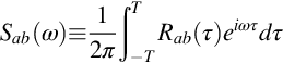
Expanding this we obtain
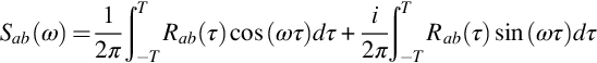
showing that Sab(ω) will, in general, be a complex function because of the probable asymmetry of Rab(τ). It is straightforward to verify that Sab will also be conjugate symmetric with frequency, so ![]() . The real and imaginary parts of Sab are referred to as the cospectrum Cab and the quad-spectrum Qab respectively.
. The real and imaginary parts of Sab are referred to as the cospectrum Cab and the quad-spectrum Qab respectively.
As one would expect, the inverse Fourier transform relates the cross spectrum back to the cross correlation

For zero time delay we obtain an expression for the covariance in terms of the cross spectral density

The conjugate symmetry of the cross spectrum ensures that quad-spectrum does not contribute to the covariance. The cospectrum may therefore be thought of as the covariance per unit frequency. Two more physically important expressions of the cross spectrum are the coherence and phase spectra, defined respectively as

and

The coherence γab2 is a squared and normalized measure of the expected value of the product of the complex amplitude of the two quantities a and b at a given frequency. If, in multiple realizations of our airfoil example, the lift (assumed say to be a compact dipole source) and sound variations (which may include background noise) were randomly phased with respect to each other implying no linear connection, then the coherence between them would be zero. If the phasing were not random, but tended to prefer a particular value, then the coherence would be positive with a value that increases the more closely correlated the signals are at that frequency. For nonzero coherence, the phase spectrum θab(ω) gives the preferred value of the phase difference, and the phase is undefined for ![]()
The coherence is an even function of frequency and is normalized so that ![]() , a value of 1 being achieved when b(t) is a constant multiple of a(t). The phase is an odd function and has a straightforward relationship to the time delay between variables. In the case of the airfoil example we argued that the positive time delay between the sound fluctuations in the far field would lead to RAB(τ) reaching its maximum magnitude at positive τ. This situation corresponds to a positive gradient of the phase spectrum θAB(ω) with frequency.
, a value of 1 being achieved when b(t) is a constant multiple of a(t). The phase is an odd function and has a straightforward relationship to the time delay between variables. In the case of the airfoil example we argued that the positive time delay between the sound fluctuations in the far field would lead to RAB(τ) reaching its maximum magnitude at positive τ. This situation corresponds to a positive gradient of the phase spectrum θAB(ω) with frequency.
A review of the above material will make it clear that the auto correlation and auto spectrum functions are simply special cases of the cross correlation and cross spectrum functions with ![]() . This is also true for the relationship between the cross spectral density and the stochastic Fourier transform. Using a derivation entirely analogous to that laid out in Eqs. (8.4.11)–(8.4.14), we can show that, for angular frequencies ω≫π/T,
. This is also true for the relationship between the cross spectral density and the stochastic Fourier transform. Using a derivation entirely analogous to that laid out in Eqs. (8.4.11)–(8.4.14), we can show that, for angular frequencies ω≫π/T,
where ![]() and
and ![]() are the Fourier transforms of a(t) and b(t). Likewise we can show, analogously to the derivation of Eq. (8.4.17) that
are the Fourier transforms of a(t) and b(t). Likewise we can show, analogously to the derivation of Eq. (8.4.17) that
Note that if one of the variables involved in the cross spectrum or correlation is a vector then these statistical measures are also vectors, e.g., the pressure velocity spectrum ![]() . If both are vectors then the resulting measures are tensors, e.g., the velocity correlation tensor
. If both are vectors then the resulting measures are tensors, e.g., the velocity correlation tensor ![]() , which is commonly abbreviated as Rij.
, which is commonly abbreviated as Rij.
8.4.3 Spatial correlation and the wavenumber spectrum
The correlation and spectral analysis techniques we have introduced to analyze the temporal behavior of a turbulent flow can equally well be applied to revealing its spatial structure. Consider turbulent velocity fluctuations u2 as a function of position along a line x1 through a turbulent flow (Fig. 8.5). The correlation between simultaneous fluctuations at two points on the line can in general be written as

If the flow is assumed homogeneous along the line (i.e., its average properties are independent of x1), then the correlation will only be a function of the separation between the two points ![]()
Homogeneity also allows us to define an integral lengthscale for the turbulence

where Lij is defined as the integral lengthscale of velocity component ui in the direction xj. We can additionally Fourier transform the correlation function in the homogeneous direction to give the wavenumber spectrum

The inverse relationship giving the correlation function in terms of the wavenumber spectrum is
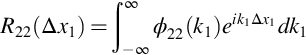
Note that, to be consistent with the Fourier transform convention introduced in Chapter 1, the signs of the exponents in the spatial Fourier transform and its inverse are reversed compared to those used with the time transform, Eqs. (8.4.1), (8.4.2). The wavenumber spectrum and spatial correlation function reveal the averaged structure of the turbulence in ways that are entirely analogous to the frequency spectrum and time correlation functions illustrated in Fig. 8.3.
The homogeneity of the turbulent flow is important in the same way that stationarity is important in time histories. Without it, the integral scale and spectrum, as well as properties derived from the spectrum, lose much of their physical meaning and mathematical utility. The assumption of homogeneity will be good if the average properties a flow vary on a scale much larger than the scale of its turbulence. For example, Fig. 8.5 depicts part of a two-dimensional turbulent boundary layer formed under a free stream in the x1 direction. The largest turbulence scales will be of the order of the boundary layer thickness δ, a distance much smaller than the scale on which the boundary layer is growing. Homogeneity in x1 is therefore a good assumption in this case. Since the boundary layer is two dimensional it would be a good approximation in the spanwise x3 direction, but not in direction x2 perpendicular to the wall.
There is much scope in the correlation and spectrum descriptors that we have not yet acknowledged. It is clear from the boundary layer example that the spatial correlation and wavenumber spectrum will be functions of x2, could also be taken in the x3 direction, and could be taken of any velocity component combination. So, we would have Lin(x2), Rij(x2,Δxn), and ϕij(x2,kn), where ![]() . Perhaps more interestingly we can expand correlations and spectra to more than one dimension. Most generally, we could consider the five-dimensional correlation between any two points in the boundary layer which has the form
. Perhaps more interestingly we can expand correlations and spectra to more than one dimension. Most generally, we could consider the five-dimensional correlation between any two points in the boundary layer which has the form
and we can envision taking the Fourier transform in △x1 and △x3 to yield the two-wavenumber spectrum

and then the Fourier transform in time to obtain the wavenumber frequency spectrum
The spectral quantities can of course always be related back to correlations through inverse Fourier transforms. So, for example, the time cross spectrum of the velocities at two points in the flow, (x1,x2,x3) and (x1′,x2′,x3′) can be obtained from the wavenumber frequency spectrum in Eq. (8.4.33) as

Descriptors like those of Eqs. (8.4.31)–(8.4.33) encompass all the possible second order statistics defined by a flow and are sufficiently rich to represent the complete acoustic source term in many linear aeroacoustic problems. Obviously, in any specific problem, the number of homogeneous directions in the flow will limit the dimensionality of the wavenumber spectrum that can be defined, just as time stationarity of the flow will determine if a physically useful frequency spectrum exists. Note that the two-point correlation, as written in the right hand side of Eq. (8.4.31), can always be defined.
Acoustic sources are often cast in terms of the fluctuating velocity field of the turbulence, but may also appear in terms of the fluctuating vorticity or the pressure on a surface, for example. In our boundary layer example, the fluctuating wall-pressure field will be characterized by the wavenumber frequency spectrum

where
Note that relationships exactly analogous to Eqs. (8.4.14), (8.4.17) exist for the wavenumber domain. Thus, for example, we can write for the wavenumber frequency spectrum of the wall-pressure,

where ![]() denotes the wavenumber frequency transform of p′. Also, we can relate the one-dimensional wavenumber spectrum to the one-dimensional wavenumber transform as,
denotes the wavenumber frequency transform of p′. Also, we can relate the one-dimensional wavenumber spectrum to the one-dimensional wavenumber transform as,

for example. In addition, by repeated application of Eq. (8.4.38) or (8.4.14) multidimensional relationships are obtained, such as,

for the planar wavenumber spectrum of the velocity fluctuations.
The combination of space and time in the correlation function and in the wavenumber frequency spectrum in general captures information about the convection or phase velocity of fluid motions as well as their scale and intensity. We can always calculate a velocity component from Δxi/τ or ω/ki. Whether such a component is physically meaningful depends on the form of the correlation or spectrum at that point. Where turbulence is carried by a mean flow, much of the energy of the flow will appear concentrated around a convective ridge.
Fig. 8.6 shows this type of feature in the pressure correlation coefficient function ![]() measured underneath a high Reynolds number turbulent boundary layer. The convective ridge defines the elongated form of the correlation function. The convection velocity Uc is calculated as Δx1/τ at the center of the ridge. For small separations Δx1, the correlation levels on the ridge are high because the turbulence does not evolve much over short distances. The slope of the convective ridge and Uc are relatively low here in the measurements (about 0.6 U∞) because the correlation includes a substantial contribution from small turbulence scales in the near-wall region where the flow speeds are slow. At larger separations the correlation values reduce as the turbulence has more distance to evolve. Smaller eddies evolve more quickly and so the correlation increasingly represents the larger eddies of the flow that are more likely to occupy faster flowing regions further from the wall. The slope of the convective ridge and Uc therefore increase for larger separations. The convection velocity of wall-pressure fluctuations in a smooth wall boundary layer is usually observed to be between 60% and 80% of the free stream velocity. The boundary layer wall-pressure spectrum and correlation function will be discussed in more detail in the next chapter.
measured underneath a high Reynolds number turbulent boundary layer. The convective ridge defines the elongated form of the correlation function. The convection velocity Uc is calculated as Δx1/τ at the center of the ridge. For small separations Δx1, the correlation levels on the ridge are high because the turbulence does not evolve much over short distances. The slope of the convective ridge and Uc are relatively low here in the measurements (about 0.6 U∞) because the correlation includes a substantial contribution from small turbulence scales in the near-wall region where the flow speeds are slow. At larger separations the correlation values reduce as the turbulence has more distance to evolve. Smaller eddies evolve more quickly and so the correlation increasingly represents the larger eddies of the flow that are more likely to occupy faster flowing regions further from the wall. The slope of the convective ridge and Uc therefore increase for larger separations. The convection velocity of wall-pressure fluctuations in a smooth wall boundary layer is usually observed to be between 60% and 80% of the free stream velocity. The boundary layer wall-pressure spectrum and correlation function will be discussed in more detail in the next chapter.

 under the boundary layer of Forest [6]. U∞=33.6 m/s, boundary layer thickness δ=231 mm. Inset shows enlargement of region at small τ and △x1. Contours are in intervals of 0.05 starting at 0.05.