
Turbulent flows
Abstract
Predictions of sound radiated as a result of the unsteady motions of a turbulent flow require estimates of the two-point space-time correlations of those flows, or their spectral equivalents. In practice these estimates are usually obtained using models developed for homogeneous and isotropic turbulence, and scaling or otherwise modifying those models to match the inhomogeneous and anisotropic reality of the application in question. The fundamental knowledge needed to do this, including the properties of homogeneous isotropic turbulence and of the most important turbulent shear flows for aeroacoustics at low Mach number, is the topic of this chapter.
Keywords
Turbulent flows; Homogeneous turbulence; Turbulent boundary layers; Wakes
In Chapter 8 it was shown that predictions of sound radiated as a result of the unsteady motions of a turbulent flow require estimates of the two-point space-time correlations of those flows, or their spectral equivalents. In practice these estimates are usually obtained using models developed for homogeneous and isotropic turbulence, and by scaling or otherwise modifying those models to match the inhomogeneous and anisotropic reality of the application in question. The fundamental knowledge needed to do this, including the properties of homogeneous isotropic turbulence and of the most important turbulent shear flows for aeroacoustics at low Mach number, is the topic of this chapter.
9.1 Homogeneous isotropic turbulence
9.1.1 Mathematical description
Homogeneous isotropic turbulence is turbulence that has average properties that are both independent of position and direction. Either one considers there to be no mean flow, or the mean flow is uniform and the turbulence is viewed from a frame of reference moving with it. Homogeneous turbulence is an ideal that can be approximated by the uniform turbulence downstream of a grid, or by Direct Navier Stokes (DNS) simulations of turbulence in periodic boxes. It is the simplest kind of turbulence and therefore the most studied and understood.
Homogeneous turbulence is decaying turbulence. Its mean flow has no shear and therefore no mechanism for the generation of new eddies from instabilities in the mean flow. At its largest scales it is therefore missing the configuration-specific biases that are present in almost all other turbulent flows. However, it serves as a useful representation of the universal components of those flows. Given Kolmogorov's hypotheses we expect this representation to become increasingly accurate at smaller scales and higher Reynolds numbers.
The value of homogeneous turbulence to aeroacoustics is not just this universal character, but also the fact that it is simple enough for analytical models of the second order statistics of the turbulence to exist. Engineers often use these models to provide acoustic source terms for flows that can be approximated by homogeneous turbulence, that average in time to something that appears homogeneous, or that are clearly neither homogeneous nor isotropic but for which no better information exists.
In analyzing homogeneous turbulence, we will consider only spatial correlations and related quantities. This is because in aeroacoustic applications it is generally assumed that the decay rate of turbulence is negligible over the time taken for the turbulence to convect over noise-producing hardware and to generate sound. Thus Taylor's hypothesis can be used to infer time dependencies from the spatial description of the turbulence.
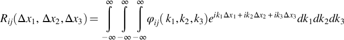
The forms of the spatial correlation function and wavenumber spectrum of the velocity fluctuations for homogeneous turbulence can be readily inferred from Eqs. (8.4.31), (8.4.32) to be
and

The inverse relationship is simply given by the equivalent inverse Fourier transform
While both Rij and φij appear to be three-dimensional tensor functions they can, in fact, both be inferred from a single one-dimensional scalar function. This can be understood if we consider the velocity fluctuations at two points A and B in a homogeneous turbulent flow, as shown in Fig. 9.1. The points are separated by a distance r and we define fluctuating velocity components us and un respectively parallel and perpendicular to the direction of separation. Isotropy means that the average flow properties must be invariant under rotation of the coordinate system used to describe them. The mean-square velocity in any direction must therefore be the same, and so ![]() . The turbulent shear stress term
. The turbulent shear stress term ![]() must also be zero as any nonzero value would reverse the sign if we rotated our coordinates 180 degrees about the axis AB in Fig. 9.1. Equivalently, we can argue that at any instant when us is positive there is equal probability that un is either positive or negative and so
must also be zero as any nonzero value would reverse the sign if we rotated our coordinates 180 degrees about the axis AB in Fig. 9.1. Equivalently, we can argue that at any instant when us is positive there is equal probability that un is either positive or negative and so ![]() . Following the same arguments, the correlation between different components at different points
. Following the same arguments, the correlation between different components at different points ![]() must also be zero. With these restrictions the only distinct correlations we can make are
must also be zero. With these restrictions the only distinct correlations we can make are ![]() and
and ![]() , the value of the latter being independent of rotation about the axis AB and thus the same for the third velocity component ut directed out of the page.
, the value of the latter being independent of rotation about the axis AB and thus the same for the third velocity component ut directed out of the page.

Given that the velocity in any other direction can be composed from these components we conclude that no other independent correlations are possible. We therefore define the longitudinal and lateral correlation coefficient functions as, respectively
where ![]() , and the associated integral scales are
, and the associated integral scales are
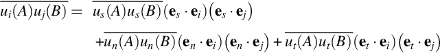
To obtain a general expression for the two-point correlation function ![]() we recognize that the Cartesian velocity components ui at A and B are simply a rotation of us, un, and ut, as shown in Fig. 9.2, and thus
we recognize that the Cartesian velocity components ui at A and B are simply a rotation of us, un, and ut, as shown in Fig. 9.2, and thus
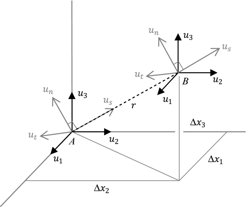
where ei denotes the unit vector in the direction of ui, and es, en, and et are the unit vectors defining the directions of us, un, and ut. We will therefore have that
Recognizing that ![]() and
and ![]() , and that the direction cosine products can be written as
, and that the direction cosine products can be written as

and
we obtain

This result is consistent with the requirement [1] that any second order isotropic tensor function must have the form ![]() where α and β are only functions of r. The additional requirement that Rij must be consistent with the incompressible continuity equation allows us to obtain a relationship between f and g. Continuity requires that
where α and β are only functions of r. The additional requirement that Rij must be consistent with the incompressible continuity equation allows us to obtain a relationship between f and g. Continuity requires that ![]() and thus, from Eq. (9.1.1),
and thus, from Eq. (9.1.1), ![]() . Applying this to Eq. (9.1.5) (noting that
. Applying this to Eq. (9.1.5) (noting that ![]() ) gives,
) gives,

See also Batchelor [1].
Substituting this expression into Eq. (9.1.4) for Lg and integrating the second term by parts gives that ![]() . Also, from Eq. (9.1.5) it follows that the sum of the normal correlation function components
. Also, from Eq. (9.1.5) it follows that the sum of the normal correlation function components
where r=(Δx1,Δx2,Δx3) and r=|r|. This function contains no reference to direction and, for ![]() , is equal to the turbulence kinetic energy κɛ.
, is equal to the turbulence kinetic energy κɛ.
To obtain a useful form of the wavenumber spectrum φij in terms of the one-dimensional description above, we first take the Fourier transform of ![]() using Eq. (9.1.2).
using Eq. (9.1.2).

where ![]() and θ is the angle between r and k. The integral over volume dΔx1dΔx2dΔx3 can instead be performed over the spherical surface defined by
and θ is the angle between r and k. The integral over volume dΔx1dΔx2dΔx3 can instead be performed over the spherical surface defined by ![]() and then with respect to r (Fig. 9.3), as
and then with respect to r (Fig. 9.3), as


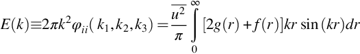
We see that ![]() depends only on wavenumber magnitude k. The total energy at a given value of k is therefore given by integrating
depends only on wavenumber magnitude k. The total energy at a given value of k is therefore given by integrating ![]() over all possible wavenumber directions, which is simply equivalent to multiplying by the spherical surface area 4πk2. This result is called the energy spectrum function and is given the symbol E(k). Thus,
over all possible wavenumber directions, which is simply equivalent to multiplying by the spherical surface area 4πk2. This result is called the energy spectrum function and is given the symbol E(k). Thus,
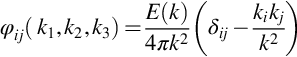
The energy spectrum function represents the turbulence kinetic energy per wavenumber. It also can be used to express the full wavenumber spectrum φij. Like Rij this is constrained to satisfy continuity and, as an isotropic tensor function, to have the form
where α(k) and β(k) are functions to be determined. Continuity implies that ![]() and therefore, from Eq. (9.1.3), that
and therefore, from Eq. (9.1.3), that ![]() . With Eq. (9.1.7) for φij this gives
. With Eq. (9.1.7) for φij this gives
Furthermore, Eq. (9.1.7) implies

Substituting α(k) and β(k) back into Eq. (9.1.7) then gives the full wavenumber spectrum as
In principle this result can also be obtained by taking the three-dimensional wavenumber transform of Eq. (9.1.5).
The energy spectrum function is conceptually useful because it is a one-dimensional function that can be used to divide the turbulence into its different scales and, as explained in Section 8.1, different physical mechanisms are expected to dominate in different scale ranges. It is therefore the natural function in which to express models of homogeneous turbulence. Below we detail and discuss two such models that are commonly used in aeroacoustics.
9.1.2 The von Kármán spectrum
In 1948, Theodore von Kármán [2] working at Caltech introduced a semiempirical model for the energy spectrum function of homogeneous turbulence based on two theoretical arguments. The first concerned Kolmogorov's hypothesis of a universal inertial subrange in turbulence where the statistical behavior of the flow is completely determined by the rate of energy flow through the cascade ɛ, as discussed in Section 8.1. This implies that ![]() in this range as a consequence of the fact that
in this range as a consequence of the fact that ![]() is the only nondimensional group that can be formed from these variables. The second argument concerned the rate of decay of the turbulence at the largest scales and indicated that
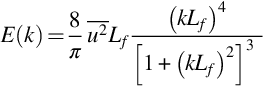
is the only nondimensional group that can be formed from these variables. The second argument concerned the rate of decay of the turbulence at the largest scales and indicated that ![]() at small wavenumbers. With these behaviors set he proposed the interpolation function
at small wavenumbers. With these behaviors set he proposed the interpolation function
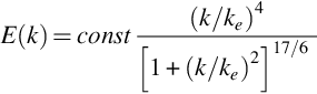
where ke is defined as the wavenumber scale of the largest eddies. The value of the constant can be fixed by requiring that E(k) integrate to the turbulence kinetic energy, giving
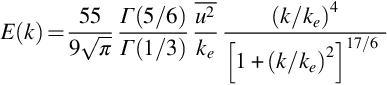
where Γ() is the Gamma function, and ke can be related to the longitudinal integral scale as

Eq. (9.1.10) can be analytically integrated into many other spectral and correlation forms, both of fundamental interest and of use in aeroacoustics problems. First we consider the planar wavenumber spectrum, obtained by taking the inverse Fourier transform of φij(k1,k2,k3) with respect to k2 and evaluating it for ![]()

This, for example, is the wavenumber spectrum of relevance to the type of problem depicted in Fig. 8.2 where an aerodynamic surface is cutting a plane through a turbulent flow and we are interested in quantitatively evaluating the scales of the turbulence in that plane. Substituting Eqs. (9.1.10), (9.1.8) into Eq. (9.1.12), we obtain

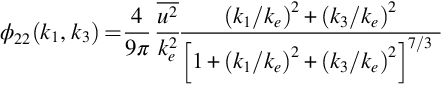
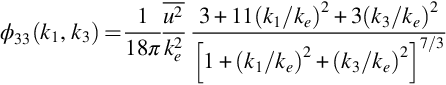
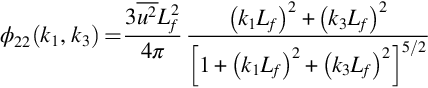
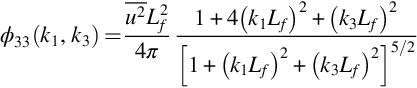
We can integrate one more time, this time with respect to k3, to give the one-dimensional wavenumber spectra along a single line through the turbulence. For ϕ11 this gives

Applying the same integral to ϕ22 and ϕ33 we obtain

Note that these are double-sided spectra. The inverse Fourier transforms of ϕ11(k1) and ϕ22(k1) with respect to k1 give the longitudinal and lateral correlation functions f and g multiplied by ![]() as functions of Δx1. Replacing Δx1 with r in those expressions gives their more general form:
as functions of Δx1. Replacing Δx1 with r in those expressions gives their more general form:

and

where K is the modified Bessel function of the second kind.
One-dimensional wavenumber spectra are of particular interest because they are easily related to the frequency spectrum that would be measured if the turbulence was convecting in the x1 direction past a fixed point. In Fig. 8.3C we plotted the turbulence frequency spectrum S11(ω) produced by boundary layer turbulence moving at ![]() over a probe. Assuming Taylor's hypothesis we can estimate this curve using a homogeneous turbulence spectrum model as
over a probe. Assuming Taylor's hypothesis we can estimate this curve using a homogeneous turbulence spectrum model as ![]() . Note that the division by U1 is necessary to ensure that S11(ω) integrates to the mean square velocity fluctuation. Fig. 9.4A shows that this prediction, made using Eq. (9.1.16) and scaled with the actual mean-square velocity and the integral scale obtained from the measured correlation functions, is remarkably accurate. The von Kármán formula only departs from the measurement at the highest frequencies where dissipation begins to affect the spectral form. Figs. 9.4B and C show similar measurements and predictions for the normal to wall and spanwise velocity spectra S22(ω) and S33(ω) at the same position in the boundary layer. The scaling of the predictions is based on the mean-square velocity and integral scale associated with each component. We see that, except in the dissipation range, the von Kármán model is quite realistic.
. Note that the division by U1 is necessary to ensure that S11(ω) integrates to the mean square velocity fluctuation. Fig. 9.4A shows that this prediction, made using Eq. (9.1.16) and scaled with the actual mean-square velocity and the integral scale obtained from the measured correlation functions, is remarkably accurate. The von Kármán formula only departs from the measurement at the highest frequencies where dissipation begins to affect the spectral form. Figs. 9.4B and C show similar measurements and predictions for the normal to wall and spanwise velocity spectra S22(ω) and S33(ω) at the same position in the boundary layer. The scaling of the predictions is based on the mean-square velocity and integral scale associated with each component. We see that, except in the dissipation range, the von Kármán model is quite realistic.
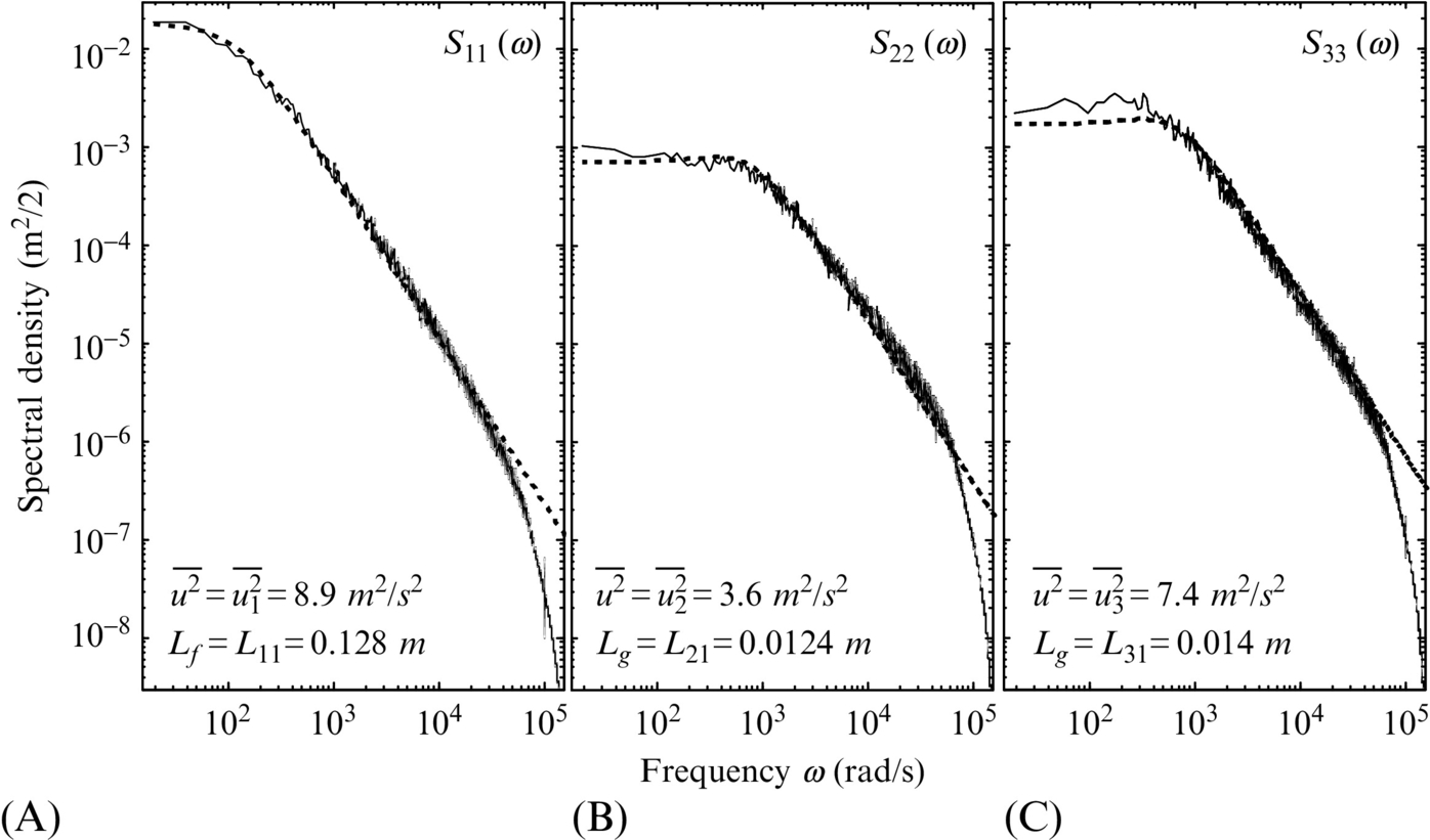
The agreement in Fig. 9.4 does not imply that the boundary layer turbulence is homogeneous and isotropic, merely that the von Kármán formula may realistically describe the form of the spectrum. Just how anisotropic the boundary layer actually is can be seen in the integral scale and velocity variance values listed in the figure. We see that ![]() is only about 40% of
is only about 40% of ![]() (instead of being equal), and that the lateral scale Lg of the u2 and u3 components is only about 10% of longitudinal scale of the u1 component Lf (as opposed to half). However, the agreement seen in the spectra of Fig. 9.4 is still significant. It tells us that we can probably make a fair estimate of the acoustic source terms in inhomogeneous anisotropic turbulent flows by assuming a von Kármán spectrum scaled on the local integral scale and turbulence intensity of the velocity component of interest. Indeed, it is on this basis that many broadband noise predictions are made.
(instead of being equal), and that the lateral scale Lg of the u2 and u3 components is only about 10% of longitudinal scale of the u1 component Lf (as opposed to half). However, the agreement seen in the spectra of Fig. 9.4 is still significant. It tells us that we can probably make a fair estimate of the acoustic source terms in inhomogeneous anisotropic turbulent flows by assuming a von Kármán spectrum scaled on the local integral scale and turbulence intensity of the velocity component of interest. Indeed, it is on this basis that many broadband noise predictions are made.
Pope [3] has extended the von Kármán interpolation formula to include a dissipation range model at high frequencies and to allow E(k) to vary as k2 at low frequencies in some situations. In its high Reynolds number form, Pope's high frequency dissipation range model involves multiplying the energy spectrum (Eq. 9.1.10) by the function
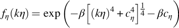
where η is the Kolmogorov lengthscale, ![]() , and
, and ![]() . Strictly speaking, since the effect of this multiplication is to lower spectral levels at the highest frequencies a slight rescaling of the numerical constant multiplying Eq. (9.1.10) then becomes necessary to ensure that the energy spectrum still integrates to the turbulence kinetic energy.
. Strictly speaking, since the effect of this multiplication is to lower spectral levels at the highest frequencies a slight rescaling of the numerical constant multiplying Eq. (9.1.10) then becomes necessary to ensure that the energy spectrum still integrates to the turbulence kinetic energy.
9.1.3 The Liepmann spectrum
Shortly after von Kármán introduced his interpolation function, his Caltech colleagues Hans Liepmann, John Laufer, and Kate Liepmann [4] proposed an alternative expression for the turbulence spectrum
At higher wavenumbers this model implies that E(k) varies as ![]() rather than the more fundamental
rather than the more fundamental ![]() . The difference can be small, however, and gives a function containing only integer powers of wavenumber that can be significantly easier to manipulate mathematically as part of aeroacoustic analyses. Integrating the Liepmann spectrum we obtain, for the planar wavenumber spectra,
. The difference can be small, however, and gives a function containing only integer powers of wavenumber that can be significantly easier to manipulate mathematically as part of aeroacoustic analyses. Integrating the Liepmann spectrum we obtain, for the planar wavenumber spectra,

and for the one-dimensional spectra,


and, finally, for the longitudinal and lateral correlation functions
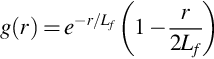
Fig. 9.5 compares the Liepmann and von Kármán interpolation formulae. The one-dimensional wavenumber spectra (Fig. 9.5A) are almost identical up to a wavenumber k/ke of about 10. The longitudinal and lateral correlation functions (Fig. 9.5B and C) are very similar. Note that for both models f(r) decays monotonically, but g(r) has a shallow overshoot at larger r so it dips below zero.

 , (B) longitudinal correlation coefficient function f(r). (C) Lateral correlation coefficient function g(r).
9.2 Inhomogeneous turbulent flows
Homogeneous isotropic turbulence is rare in practical applications. Aeroacousticians are almost always dealing with turbulent flows with average properties that vary substantially across their width and that involve motions with a clear preference for direction. The specifics of these vary from configuration to configuration making a single prescription impossible. However, turbulence only forms in the rotational regions of a flow where viscous action has had an influence. Thus a substantial proportion of the turbulent flows of interest are wakes or boundary layers. In this section we describe these flows in their most idealized form; the fully developed plane wake and the zero-pressure gradient flat plate turbulent boundary layer. The goal here is to give the reader a qualitative and quantitative understanding of these canonical flows that they can then adapt and extend when faced with aeroacoustic sources generated by more configuration-specific turbulent shear flows.
It is important to state at the outset that no analytic interpolation formulae for the velocity correlations exist for these flows. Comprehensive numerical characterizations of the correlation functions (either measured or computed) exist in only a few cases and are too unwieldy to be used for routine aeroacoustic analysis. Instead, such analysis must usually rely on scaling of von Kármán or Liepmann spectra to the local or spatially averaged properties of these flows. Therefore it is these properties—the Reynolds stress fields, the velocity scales, and the lengthscales—that we will highlight in our discussion. Where visible, we also point out features of the large-scale turbulence structure that are unlikely to be modeled well with homogeneous turbulence spectra. Interpolation formulae do exist for the wavenumber-frequency spectrum of the wall-pressure fluctuations of the turbulent boundary layer. These models, which are central to the aeroacoustic analysis of noise from flow over surfaces, will be presented at the end of this section.
9.2.1 The fully developed plane wake
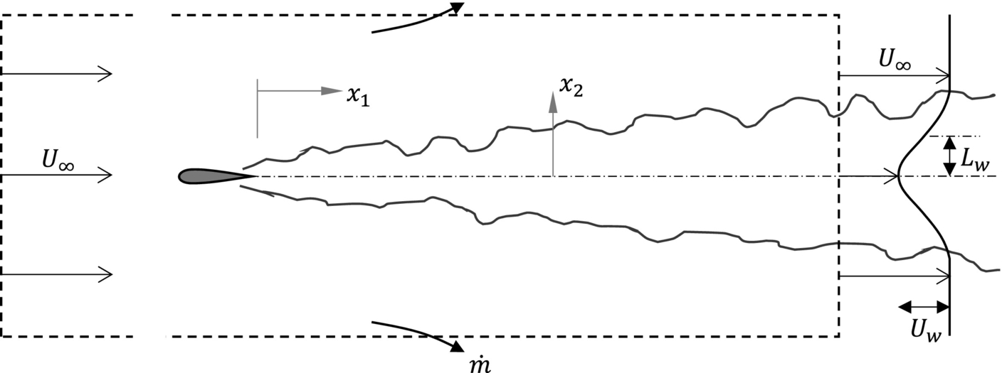
Consider a two-dimensional body, such as an airfoil or strut, placed in a free stream as shown in Fig. 9.6. The body disturbs the flow causing the formation of a wake that trails downstream. After an initial period of comparatively rapid evolution the wake settles down into a slender flow with almost parallel mean streamlines in which gradients in the flow direction ![]() are much less than those across the wake
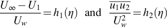
are much less than those across the wake ![]() . This fully developed far wake is the focus of our interest here. The mean-velocity profile of the far wake has a symmetric form characterized by Uw, the maximum velocity deficit reached on the wake centerline, and Lw, the distance measured from the wake centerplane to the point where the deficit is half Uw. It is usual to refer to LW as the half wake width.
. This fully developed far wake is the focus of our interest here. The mean-velocity profile of the far wake has a symmetric form characterized by Uw, the maximum velocity deficit reached on the wake centerline, and Lw, the distance measured from the wake centerplane to the point where the deficit is half Uw. It is usual to refer to LW as the half wake width.
At high Reynolds number, no scales beyond Uw and Lw are needed to characterize the mean flow or the important turbulence scales. Viscous scales are only important in controlling the dissipation of the energy of the smallest turbulence and have no direct influence on the overall flow structure. Thus the flow reaches a self-similar state in which the mean flow, turbulence stresses, spectra, and correlations can all be described by functions that are independent of streamwise position. For example, using the coordinate system of Fig. 9.6, we expect ![]() ,
, ![]() , Li1/Lw, and Li3/Lw; all to be only functions of
, Li1/Lw, and Li3/Lw; all to be only functions of ![]() (where Lij is defined as the integral lengthscale of velocity component ui in the direction xj). The distances defining two point correlations (and wavenumbers) are also expected to scale on Lw. Frequencies seen at a fixed point will scale closely as
(where Lij is defined as the integral lengthscale of velocity component ui in the direction xj). The distances defining two point correlations (and wavenumbers) are also expected to scale on Lw. Frequencies seen at a fixed point will scale closely as ![]() since fluctuations are produced by eddies being convected past the point almost at
since fluctuations are produced by eddies being convected past the point almost at ![]() . Note that
. Note that ![]() in the far wake.
in the far wake.
The fact that the form of the wake becomes invariant with streamwise position does not imply that this flow is universal. Fully developed wakes generated by different bodies are qualitatively very similar, but the relative magnitudes of such things as the peak turbulence intensity ![]() to the maximum deficit Uw may differ by as much as 30% [5].
to the maximum deficit Uw may differ by as much as 30% [5].
We can infer how the controlling scales Uw and Lw change as the wake grows. Consider first the control volume shown in Fig. 9.6. Assuming incompressible flow and requiring that the mass flow in and out of the volume be the same, we have
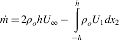
where ![]() and h are the x2 limits of the control volume and
and h are the x2 limits of the control volume and ![]() is the mass flow per unit span out of the top and bottom faces of the volume. Equating the difference in the momentum flow into and out of the control volume in the x1 direction to the drag force per unit span on the body as D, gives
is the mass flow per unit span out of the top and bottom faces of the volume. Equating the difference in the momentum flow into and out of the control volume in the x1 direction to the drag force per unit span on the body as D, gives

where we are assuming that the mass flow ![]() leaves the volume with a U1 velocity component equal to the free-stream velocity—a good approximation if h is large. Substituting for
leaves the volume with a U1 velocity component equal to the free-stream velocity—a good approximation if h is large. Substituting for ![]() and normalizing on
and normalizing on ![]() this expression simplifies to
this expression simplifies to
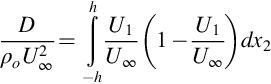
The integral on the right-hand side has units of distance and is referred to as the momentum thickness θ. Since it is equal to the normalized drag it must be invariant with streamwise position in the wake x1. Note that the Eq. (9.2.3) can be written as ![]() , where Cd is the two-dimensional drag coefficient on the body and c is the reference length used to normalize Cd, such as airfoil chord.
, where Cd is the two-dimensional drag coefficient on the body and c is the reference length used to normalize Cd, such as airfoil chord.
Writing the integrand of Eq. (9.2.3) as ![]() , we note that
, we note that ![]() will scale with
will scale with ![]() , and
, and ![]() since
since ![]() . Similarly x2 will scale with Lw. We must therefore have that
. Similarly x2 will scale with Lw. We must therefore have that ![]() , and thus the product of the velocity and length scales of the wake must be constant.
, and thus the product of the velocity and length scales of the wake must be constant.
To determine how these parameters vary individually, we use the streamwise component of the Reynolds averaged Navier Stokes equations (8.3.4). For two-dimensional mean flow with ![]() and ignoring viscous terms this is, for i=1
and ignoring viscous terms this is, for i=1

A formal order of magnitude analysis [6] shows that only the first term on the left hand side and the last term on the right hand side are significant in the far wake, giving
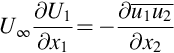
where the substitution of ![]() for U1 on the left hand side follows from
for U1 on the left hand side follows from ![]() . Following Townsend [7], we can use the concept of self similarity to scale the flow in the wake. This requires the velocity profile to scale on the wake width LW. Given that θ=UWLW/U∞ is constant, this also requires scaling of the wake velocity deficit on UW. Consequently, we can write the mean velocity and stress profiles as a functions of η=x2/LW in the form
. Following Townsend [7], we can use the concept of self similarity to scale the flow in the wake. This requires the velocity profile to scale on the wake width LW. Given that θ=UWLW/U∞ is constant, this also requires scaling of the wake velocity deficit on UW. Consequently, we can write the mean velocity and stress profiles as a functions of η=x2/LW in the form
It follows that
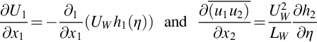
Substituting these into Eq. (9.2.5), recognizing that ![]() , and rearranging gives
, and rearranging gives
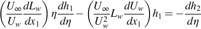
Since the terms outside the parentheses are not functions of x1, the terms inside the parentheses must be constants and this gives two simultaneous differential equations for Lw and Uw. The solution to these is simply that ![]() and
and ![]() where n is a constant. Since we already know that
where n is a constant. Since we already know that ![]() is a constant then we must have that
is a constant then we must have that ![]() and
and ![]() .
.
This is realized in practice. For example, Fig. 9.7 shows data from the plane wake shed from a roughened airfoil in a uniform air flow [8], much as pictured in Fig. 9.6. The airfoil is 0.2 m in chord and the free-stream velocity ![]() is 20 m/s, for a Mach number of 0.059 and a Reynolds number
is 20 m/s, for a Mach number of 0.059 and a Reynolds number ![]() . The drag coefficient on the airfoil is 0.0187 implying
. The drag coefficient on the airfoil is 0.0187 implying ![]() . The scaling variables are shown as a function of x1/θ where x1 is measured downstream from the wake origin, very close to the airfoil trailing edge. After some slight initial adjustment, Uw and Lw closely follow square root variations predicted. The specific dependencies shown by the dotted lines in Fig. 9.12 are;
. The scaling variables are shown as a function of x1/θ where x1 is measured downstream from the wake origin, very close to the airfoil trailing edge. After some slight initial adjustment, Uw and Lw closely follow square root variations predicted. The specific dependencies shown by the dotted lines in Fig. 9.12 are;
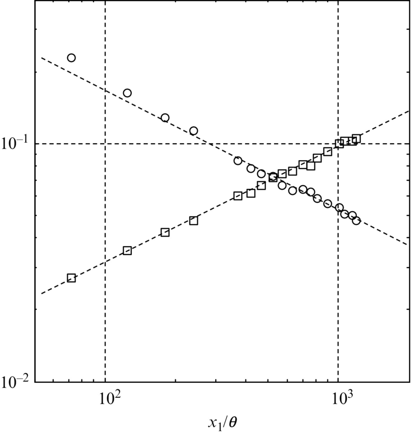
The ratio between θ/Lw and Uw/U∞, of 1.97 is expected to be universally constant [5]. This wake develops a self-similar structure by about eight chord lengths (860θ) downstream of the trailing edge. In Figs. 9.8–9.11 we show the self-similar form so as to illustrate the typical structure of a fully developed wake. Mean velocity and Reynolds-stress profiles are plotted in Fig. 9.8. The mean-velocity profile is an inverted bell shape that has an almost Gaussian form. The curve fit of Wygnanski et al. [5]
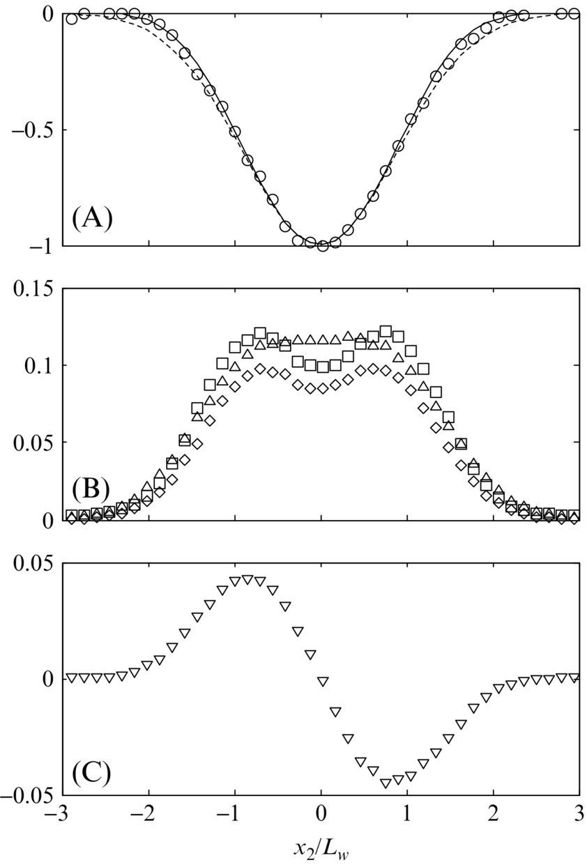
 ; ▽,
; ▽, ; ⋄,
; ⋄, . (C) Turbulence shear stress; △,
  .
.

provides a quite accurate model of the mean profile with the only effect of the (x2/Lw)4 term in the exponent being to slightly narrow the tails of the profile (Fig. 9.8A).
The Reynolds normal stresses (Fig. 9.8B) are almost constant and equal over the central portion of the wake ![]() where they reach values of about 0.1Uw2. They fall below 10% of this value just over two wake half-widths from the center. The Reynolds shear stress
where they reach values of about 0.1Uw2. They fall below 10% of this value just over two wake half-widths from the center. The Reynolds shear stress ![]() forms an antisymmetric profile that roughly mirrors the negative of the gradient of the mean velocity. It reaches its peak magnitude of just over 0.04, near
forms an antisymmetric profile that roughly mirrors the negative of the gradient of the mean velocity. It reaches its peak magnitude of just over 0.04, near ![]() . Note that two-dimensionality implies that the other Reynolds shear stresses
. Note that two-dimensionality implies that the other Reynolds shear stresses ![]() and
and ![]() are zero.
are zero.
Fig. 9.9 shows the integral lengthscales in the flow. The flow is homogeneous in the spanwise x3 direction and almost homogeneous in the streamwise x1 direction, since it is slowly growing. We can therefore define meaningful integral scales of each of the three velocity components in x1 and x3, and these integral scales are functions of the position in the wake x2/Lw. Recall that, in the convention established in Section 8.4, Lin denotes the lengthscale of velocity component ui taken in direction xn. The streamwise lengthscales in Fig. 9.9B were measured by determining the integral timescale from time-delay correlations, and then applying Taylor's hypothesis. We expect this to be a good assumption since ![]() and so the mean velocity is always close to
and so the mean velocity is always close to ![]() and the timescale on which the turbulence evolves Lw/Uw is therefore much longer than the timescale for it to convect past a fixed point
and the timescale on which the turbulence evolves Lw/Uw is therefore much longer than the timescale for it to convect past a fixed point ![]() .
.
In many ways the lengthscale profiles of Fig. 9.9 have similar shapes to those of the turbulence normal stresses, with roughly constant regions over the middle 50% or so of the wake flanked by regions of decay towards the edges. The lengthscales reveal strong anisotropy of the largest scale eddies in the wake. Near the wake center the longitudinal lengthscale in the streamwise direction L11 (Fig. 9.9B) is about 80% of the half-wake width and about four times the two lateral scales L21 and L31 (recall that for homogeneous turbulence the longitudinal scale is twice the lateral). At the same position, the longitudinal scale in the spanwise direction L33 (Fig. 9.9A) is about 0.4Lw and actually smaller (by about 30%) than the lateral scale L23.
The nature of the large-scale eddies producing this behavior is more apparent in the spanwise and streamwise correlation coefficient functions from which the lengthscales are integrated. Fig. 9.10 shows these functions at the wake center, ![]() . The streamwise correlation (Fig. 9.10B) of the vertical velocity component ρ22 is seen to oscillate as it decays reaching a minimum at
. The streamwise correlation (Fig. 9.10B) of the vertical velocity component ρ22 is seen to oscillate as it decays reaching a minimum at ![]() followed by a shallow maximum at
followed by a shallow maximum at ![]() . The negative area produced by the overshoot results in the comparatively low integral lengthscale L21 at the wake center. The oscillation indicates some regularity in the spacing of eddies in the streamwise direction, termed quasi periodicity. What we are seeing is organization associated with eddies generated directly from the roll up of the shear visible in the mean-velocity profile pictured in Fig. 9.8A, a feature that would not be represented well with a Liepmann or von Kármán model (Fig. 9.4C), even though such a model might still adequately describe the smaller scales. These large scale organized motions may also be responsible for the broad wings seen in the spanwise decay of ρ22 visible in Fig. 9.10A.
. The negative area produced by the overshoot results in the comparatively low integral lengthscale L21 at the wake center. The oscillation indicates some regularity in the spacing of eddies in the streamwise direction, termed quasi periodicity. What we are seeing is organization associated with eddies generated directly from the roll up of the shear visible in the mean-velocity profile pictured in Fig. 9.8A, a feature that would not be represented well with a Liepmann or von Kármán model (Fig. 9.4C), even though such a model might still adequately describe the smaller scales. These large scale organized motions may also be responsible for the broad wings seen in the spanwise decay of ρ22 visible in Fig. 9.10A.

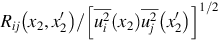
The inhomogeneity of the wake in the x2 direction means that the spatial correlation in this direction is a function of two positions x2 and x2′ and not just the distance between them. Fig. 9.11 shows this two-dimensional correlation function Rij(x2,x2′), for zero Δx1, Δx3 and τ, plotted in coefficient form by normalizing on the geometric average of the corresponding mean-square velocity fluctuations at x2 and x2′. In this normalization the diagonals of the contour maps in Fig. 9.11 have a value of unity and the rate of decay to either side is an indication of the extent of the correlation perpendicular to the plane of the wake. For example, Fig. 9.11A shows that streamwise velocity fluctuations at the wake center correlate over about one half-wake width above and below the center. The vertical extent of the correlation in the region of highest mean-velocity gradient near ![]() is actually larger than at the centerline, giving the correlation map a waisted appearance. Otherwise the vertical extent of the correlations of all three velocity components is remarkably constant with the position in the wake, with the vertical velocity component u2 correlating over the greatest distance, and the spanwise correlation u3 the smallest. We can therefore define meaningful integral scales in the x2 direction. Integrating the correlation coefficient function, as shown in Fig. 9.11 with respect to x2′ for
is actually larger than at the centerline, giving the correlation map a waisted appearance. Otherwise the vertical extent of the correlations of all three velocity components is remarkably constant with the position in the wake, with the vertical velocity component u2 correlating over the greatest distance, and the spanwise correlation u3 the smallest. We can therefore define meaningful integral scales in the x2 direction. Integrating the correlation coefficient function, as shown in Fig. 9.11 with respect to x2′ for ![]() we obtain scales of 0.35Lw, 0.82Lw, and 0.17Lw for the u1, u2, and u3 velocity components respectively.
we obtain scales of 0.35Lw, 0.82Lw, and 0.17Lw for the u1, u2, and u3 velocity components respectively.

 for the wake. (A) Streamwise velocity i=j=1, (B) normal velocity i=j=2, (C) spanwise velocity i=j=3. Contours in steps of 0.1: —, Positive levels;
  , zero level. Data from Ref. [8].
9.2.2 The zero pressure gradient turbulent boundary layer
Any surface exposed to a high Reynolds number air stream will develop a boundary layer. The boundary layer is an expression of the no-slip condition imposed at the surface, which requires that the fluid layer immediately adjacent to a surface not move relative to it. At low Mach numbers the no-slip condition, and the boundary layer it produces, are the only sources of vorticity within a flow. Wakes, regions of separation and vortical flows, all originate from boundary layers.
Boundary layers are by definition thin. That is, thin relative to the streamwise distance over which the boundary layer grows significantly, and thin compared to the local radius of curvature of the surface. A boundary layer is therefore another example of a slender flow with almost parallel streamlines in which gradients of the average velocity properties in the flow direction are much less than those across the boundary layer. The almost parallel streamlines also ensure that the mean pressure is constant across the boundary layer, and that pressure variations in the streamwise direction are impressed by the overriding irrotational flow. We refer to the streamwise pressure gradient as favorable or adverse depending, respectively on whether it is tending to accelerate or decelerate the fluid.
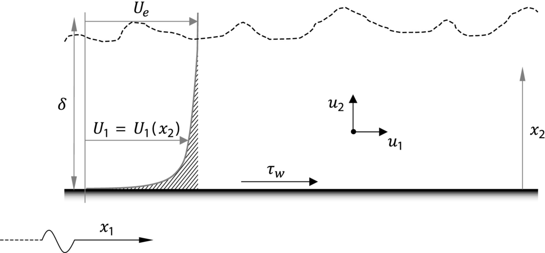
Fig. 9.12 shows the coordinate set up for our boundary layer discussion, with x1 measured streamwise from the origin of the boundary layer far upstream, x2 perpendicular to the wall, and x3 spanwise. The velocity of the irrotational flow just outside the boundary layer edge is Ue and the time mean frictional stress exerted by the boundary layer on the wall is τw. We define the local friction coefficient ![]() . We denote the boundary layer thickness as δ and this is defined as the distance from the wall to the point where the mean-velocity U1 is 99% of Ue. We also define a boundary layer momentum thickness,
. We denote the boundary layer thickness as δ and this is defined as the distance from the wall to the point where the mean-velocity U1 is 99% of Ue. We also define a boundary layer momentum thickness,
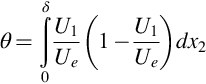
Similar to the wake, the momentum thickness is related to viscous drag. Specifically, a control volume analysis similar to the analysis for the wake in Section 9.2.1 relates the incremental increase in the normalized friction drag per unit length to twice the incremental increase in momentum thickness per unit length, ![]() . A second integral measure of the boundary layer thickness is the displacement thickness δ⁎.
. A second integral measure of the boundary layer thickness is the displacement thickness δ⁎.

This is a measure of the loss of volumetric flow rate in the boundary layer per unit span due to the frictional slowing of the flow. Graphically it is equivalent to the shaded area outside the mean-velocity profile shown in Fig. 9.12 divided by Ue. The slower flow rate in the boundary layer effectively pushes the overriding irrotational flow away from the wall by a distance equal to δ⁎.
A smooth surface exposed to a low-turbulence free stream will first develop a laminar boundary layer, but transition to a turbulent flow occurs relatively quickly at most Reynolds numbers of engineering relevance. A typical length Reynolds number x1Ue/ν for transition to turbulence with zero pressure gradient is about 600,000 implying, for example, transition within about 10 cm in an air flow of 100 m/s. Transition can occur much sooner in the presence of surface roughness, significant free-stream turbulence, or an adverse pressure gradient, or can be delayed substantially in a favorable pressure gradient or if the free stream is particularly clean.
At high Reynolds numbers a turbulent boundary layer contains a vast range of eddy sizes, from those that encompass the whole boundary layer to microscopic motions that dissipate energy directly to viscosity. Away from the wall the largest eddies are responsible for an intricately convoluted boundary layer edge, beneath which a full turbulent energy cascade is established. Close to the wall, however, the extreme velocity gradients associated with the no-slip condition produce instability and roll up of new turbulent eddies so small as to be comparable to that of the energy dissipating motions. The presence of the wall thus enforces some spatial sorting of the turbulence structure.
In a zero pressure gradient turbulent boundary layer two sets of scales are needed to describe the mean flow and average turbulence properties. Close to the wall the flow is determined by viscosity ν and the wall shear stress τw from which we can form the “inner” velocity and length scales ![]() and ν/uτ. Note that uτ is referred to as the friction velocity. The flow near the boundary layer edge is also determined by the friction (but with no direct dependence on viscosity) as well as the boundary layer thickness and so the “outer” scales here are uτ and δ. As we will see below, the edge velocity Ue also plays some role throughout the boundary layer.
and ν/uτ. Note that uτ is referred to as the friction velocity. The flow near the boundary layer edge is also determined by the friction (but with no direct dependence on viscosity) as well as the boundary layer thickness and so the “outer” scales here are uτ and δ. As we will see below, the edge velocity Ue also plays some role throughout the boundary layer.
Accurate and fast computational methods for boundary layer calculation, with and without pressure gradient, are well established and readily available [9,10]. For zero pressure gradient turbulent boundary layers a number of empirical formulae exist as well. The skin-friction coefficient

can be estimated using the well-known Schulz-Grunow formula
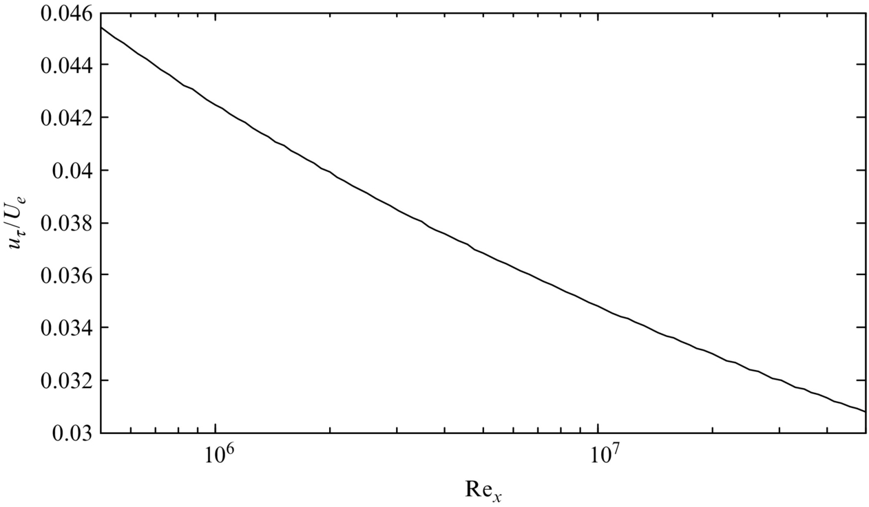
where ![]() . Note that many other curve fits exist [11]. In Fig. 9.13 this expression has been used to plot the variation in uτ/Ue with Reynolds number. The normalized friction velocity and the skin-friction coefficient gently decrease with an increase in Reynolds number, and uτ/Ue is close to 4% for Reynolds numbers between about 1 and 4 million (this Reynolds number range encompasses most wind tunnel work and some full-scale applications, such as wind turbines). Simple calculations for the boundary layer thicknesses can be obtained by approximating the mean-velocity profile using a 1/7th power-law curve [12] to give:
. Note that many other curve fits exist [11]. In Fig. 9.13 this expression has been used to plot the variation in uτ/Ue with Reynolds number. The normalized friction velocity and the skin-friction coefficient gently decrease with an increase in Reynolds number, and uτ/Ue is close to 4% for Reynolds numbers between about 1 and 4 million (this Reynolds number range encompasses most wind tunnel work and some full-scale applications, such as wind turbines). Simple calculations for the boundary layer thicknesses can be obtained by approximating the mean-velocity profile using a 1/7th power-law curve [12] to give:

with ![]() and
and ![]() . Eq. (9.2.13) implies that the boundary layer thickness grows almost linearly as x14/5, and has a thickness of roughly equal to 2% of its running length. Favorable and adverse pressure gradients will result in thinner and substantially thicker boundary layer thicknesses, respectively.
. Eq. (9.2.13) implies that the boundary layer thickness grows almost linearly as x14/5, and has a thickness of roughly equal to 2% of its running length. Favorable and adverse pressure gradients will result in thinner and substantially thicker boundary layer thicknesses, respectively.
As Eqs. (9.2.12), (9.2.13) imply, the ratios of the micro and macro turbulent boundary layer scales uτ/Ue and ν/uτδ are not constant. This means that, unlike the wake, the turbulent boundary layer does not reach a self-similar state. Instead it continually sustains two distinct scaling regions. This is particularly apparent for the mean-velocity profile. In the outer region the slowing of the mean flow relative to the free-stream scales with the friction and distances scale on the boundary layer thickness, so

This is known as the “law of the wake.” In the inner region, adjacent to the wall, only the friction and viscosity determine the flow:
where the inner variables are defined as ![]() and
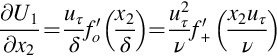
and ![]() . This is “the law of the wall.” Obviously, these two descriptions of the profile must be consistent and presumably, must overlap. If so, the mean-velocity gradients implied by Eqs. (9.2.14), (9.2.15) must match in the overlap region and we have
. This is “the law of the wall.” Obviously, these two descriptions of the profile must be consistent and presumably, must overlap. If so, the mean-velocity gradients implied by Eqs. (9.2.14), (9.2.15) must match in the overlap region and we have
and thus
Since they are functions of different nondimensional variables, the left and right hand sides of this equation can only be the same if they are both equal to a constant, defined as 1/κ. Integrating ![]() in Eq. (9.2.17) we a have
in Eq. (9.2.17) we a have
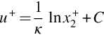
where κ is referred to as the von Kármán constant. We see that the overlap portion of the profile must have a semilogarithmic form and this is indeed observed in practice. There is no universal agreement as to the exact values of the constants κ and C, though most authors choose values close to 0.40 and 4.9, respectively.
The structure of the entire mean-velocity profile is illustrated in Fig. 9.14 which includes experimental data from a flat plate boundary layer with a momentum-thickness Reynolds number Reθ=θUe/ν of 15,500 [13]. Fig. 9.14A shows the profile plotted in terms of x2+ and on a semilogarithmic scale to more clearly show the near-wall behavior. We see that the law of the wall consists of three regions. For ![]() less than about 5 the profile approaches the linear form u+=x2+ with a slope set by the velocity gradient at the wall. This is called the linear sublayer. In the buffer layer, between about x2+=5 and 30, the profile transitions to the semilogarithmic form of Eq. (9.2.18).
less than about 5 the profile approaches the linear form u+=x2+ with a slope set by the velocity gradient at the wall. This is called the linear sublayer. In the buffer layer, between about x2+=5 and 30, the profile transitions to the semilogarithmic form of Eq. (9.2.18).

Both sublayer and buffer layer portions of the profile can be estimated by integrating the van Driest [14] formulation

from the wall, with ![]() . The semilogarithmic region, or log layer, is also part of the law of the wake and extends, approximately from
. The semilogarithmic region, or log layer, is also part of the law of the wake and extends, approximately from ![]() to
to ![]() . In the outer region, beyond
. In the outer region, beyond ![]() , the profile curves over to meet with the free stream. The form of the profile in the semilogarithmic and outer regions is often estimated by using Coles [15] extension of Eq. (9.2.18)
, the profile curves over to meet with the free stream. The form of the profile in the semilogarithmic and outer regions is often estimated by using Coles [15] extension of Eq. (9.2.18)
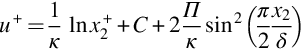
where ![]() .
.
The profiles of the turbulence stresses also have two scaling regions, in the inner region varying as ![]() and as x2/δ in the outer region. The stresses
and as x2/δ in the outer region. The stresses ![]() ,
, ![]() ,
, ![]() , and
, and ![]() are generally taken to scale with uτ2 over the whole boundary layer, though this is a matter of some debate. In particular, it is fairly clear that the peak nondimensional streamwise turbulence normal stress
are generally taken to scale with uτ2 over the whole boundary layer, though this is a matter of some debate. In particular, it is fairly clear that the peak nondimensional streamwise turbulence normal stress ![]() increases significantly with Reynolds number [16] and it has been proposed that
increases significantly with Reynolds number [16] and it has been proposed that ![]() scales on uτUe [17]. This is believed to result from “inactive” motion on the boundary layer—essentially velocity fluctuations in the u1 component driven by large-scale irrotational motions in the outer part of the boundary layer [18].
scales on uτUe [17]. This is believed to result from “inactive” motion on the boundary layer—essentially velocity fluctuations in the u1 component driven by large-scale irrotational motions in the outer part of the boundary layer [18].
Fig. 9.15 shows sample turbulence stress profiles for the same Reθ=15,500 boundary layer represented in Fig. 9.14. The boundary layer thickness is based on a statistical average quantity and thus the instantaneous boundary layer edge often exceeds this height. As a result, the turbulence stresses (Fig. 9.15) are not completely zero outside the boundary layer edge. At ![]() the normal stresses are about 0.004 Ue2 (2% turbulence intensity). Turbulence levels intensify as the wall is approached, and become increasingly anisotropic, with the streamwise normal stress
the normal stresses are about 0.004 Ue2 (2% turbulence intensity). Turbulence levels intensify as the wall is approached, and become increasingly anisotropic, with the streamwise normal stress ![]() becoming roughly twice the spanwise
becoming roughly twice the spanwise ![]() and wall-normal
and wall-normal ![]() stresses. While not visible in the figure,
stresses. While not visible in the figure, ![]() peaks very close to the wall towards the bottom of the buffer layer, whereas
peaks very close to the wall towards the bottom of the buffer layer, whereas ![]() and
and ![]() reach almost constant maximum values in the semilogarithmic region of the mean-velocity profile (Fig. 9.15). In particular, the shear-stress
reach almost constant maximum values in the semilogarithmic region of the mean-velocity profile (Fig. 9.15). In particular, the shear-stress ![]() is constant here with a value equal to half the skin friction coefficient Cf.
is constant here with a value equal to half the skin friction coefficient Cf.

 ; ▽,
; ▽,  ; ◇,
; ◇,  . (B) Turbulence shear stress; △,
  . Data from Ref. [38].
This equivalence derives from the average streamwise momentum Eq. (8.3.4) which in the inner region can be shown [9] to reduce to the statement that the sum of the turbulent and viscous shear stresses in the inner region is constant and equal to the wall shear stress:
Thus, ![]() is constant in the log layer, where viscous effects are insignificant, and decreases in the buffer layer to balance the increase in viscous shear.
is constant in the log layer, where viscous effects are insignificant, and decreases in the buffer layer to balance the increase in viscous shear.
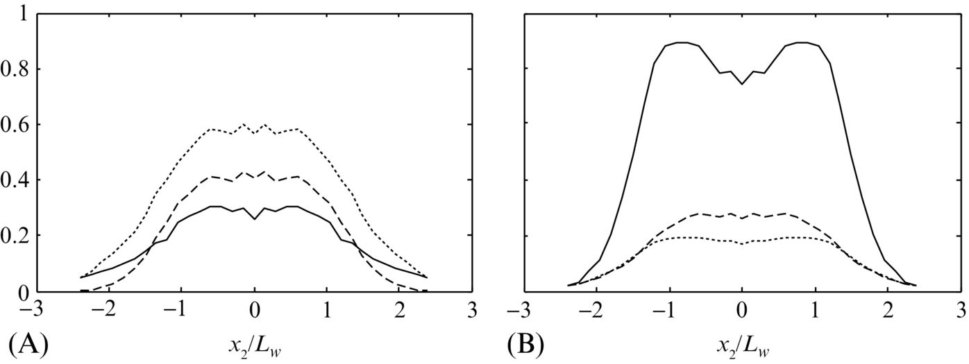
The size and form of the largest eddies responsible for the velocity fluctuations are, to some extent, revealed in Figs. 9.16 and 9.17. Fig. 9.16A shows the integral timescale associated with each of the three velocity components as a function of distance from the wall. Sample time delay correlation functions from which these scales were obtained are shown in Figs. 9.17A through C. Fig 9.16B shows integral lengthscales in the spanwise direction as a function of x2 with example correlation functions appearing in Figs. 9.17D through F.
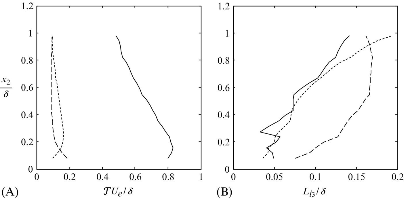
 for: —, u1; ---, u2; −−, u3. (B) Spanwise integral lengthscales: —, L13/δ; ---, L23/δ; −−, L33/δ. Data from Ref. [38].
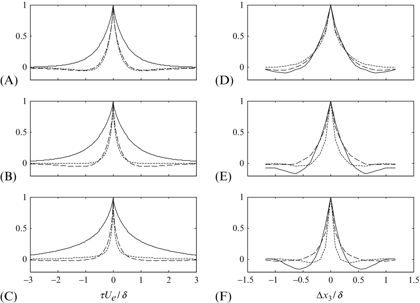
The integral timescales (Fig. 9.16A), are approximately constant or increase slowly as the boundary layer is traversed from top down. Close to the wall, in the region not shown in Fig. 9.16A, the timescales are expected to become proportional to distance from the wall [19] and thus reduce to zero. By far the largest timescale and therefore, through the qualitative application of Taylor's hypothesis, the largest streamwise lengthscale is that associated with the streamwise velocity fluctuations u1. This scale is about five times that associated with the spanwise and wall normal velocity fluctuations. The underlying time-delay correlation coefficient functions (Fig. 9.17A–C) show that this is because ρ11 has very long positive tails, indicating significant correlation for time delays as large as 3δ/Ue (the time taken for the flow at the boundary layer edge to move downstream by three boundary layer thicknesses). The ρ22 and ρ33 correlations have less pronounced tails and for ![]() those tails are negative and thus subtract from the corresponding integral scales.
those tails are negative and thus subtract from the corresponding integral scales.
The spanwise integral lengthscales (Fig. 9.16B) are quite small compared to the implied streamwise scales and are seen to increase with distance from the wall in the outer region. Over most of the boundary layer the lengthscale of the spanwise velocity fluctuations L33 is largest and reaches a value of some 17% of δ over the top half of the boundary layer. However, the associated correlation coefficient functions (Fig. 9.17D–F) show that the streamwise velocity component u1 actually correlates over larger spanwise distances than u3. The streamwise velocity correlation function ρ11 has negative lobes, however, for larger spanwise separations that reduce its integral scale. The negative lobes are more pronounced towards the bottom of the boundary layer.
As with the plane wake, the inhomogeneity of the boundary layer means that the spatial correlation in the vertical direction is a function of two positions x2 and x2′ and not just the distance between them. This correlation coefficient function ![]() is plotted in Fig. 9.18. This figure shows that streamwise velocity fluctuations in the log layer near the wall have about a 10% correlation coefficient with those at the mid height of the boundary layer, and that streamwise velocity fluctuations at the mid height correlate measurably with those over almost the entire boundary layer thickness. The scale of the vertical correlation of u1 appears almost independent of position in the boundary layer. This contrasts with the scale of the correlation of normal-to-wall fluctuations u2 which grows approximately linear with distance from the wall (Fig. 9.18B). The spanwise velocity correlation also grows with distance from the wall (Fig. 9.18C), but this velocity component is the least well correlated in the vertical direction.
is plotted in Fig. 9.18. This figure shows that streamwise velocity fluctuations in the log layer near the wall have about a 10% correlation coefficient with those at the mid height of the boundary layer, and that streamwise velocity fluctuations at the mid height correlate measurably with those over almost the entire boundary layer thickness. The scale of the vertical correlation of u1 appears almost independent of position in the boundary layer. This contrasts with the scale of the correlation of normal-to-wall fluctuations u2 which grows approximately linear with distance from the wall (Fig. 9.18B). The spanwise velocity correlation also grows with distance from the wall (Fig. 9.18C), but this velocity component is the least well correlated in the vertical direction.

 for a flat plate turbulent boundary layer at Reθ=15,500. (A) Streamwise velocity i=j=1, (B) Normal velocity i=j=2, (C) Spanwise velocity i=j=3. Contours in steps of 0.1; —, Positive levels;
  , zero level; ---, negative levels. Data from Ref. [38].
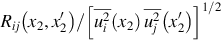
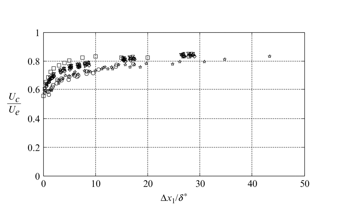
Convection velocities of the velocity fluctuations of the turbulence in the boundary layer are a function of distance from the wall x2. For most of the boundary layer, the convection velocity Uc measured from the streamwise space-time correlation is close to the local mean-velocity [20] However, in the buffer layer and linear sublayer the convection velocity becomes almost constant at between 10 and 15 uτ indicating, perhaps, that the streamwise velocity correlations in this region are predominantly generated by the overriding turbulent structures, rather than by eddies contained within these regions. A bulk convection velocity for the boundary layer turbulence, which is of particular relevance to aeroacoustic applications, can be defined using the streamwise space-time correlation wall-pressure fluctuations. As will be explained in the next section, the pressure fluctuations represent an integral over the boundary layer thickness. Fig. 9.19 shows convection velocities deduced from the wall-pressure correlations over streamwise separations Δx1 for a range of momentum-thickness Reynolds numbers [20–23]. For the smallest streamwise separations, for which the correlation contains the greatest contribution from small scale eddies near the wall, Uc is close to 0.6Ue. At large separations, where the correlation is mostly determined by the largest eddies, Uc is between about 0.8Ue and 0.85Ue. Note that there is some scatter in the rate of increase with spacing between studies that may indicate a slight increasing trend with Reynolds number.
9.2.3 The turbulent boundary layer wall-pressure spectrum
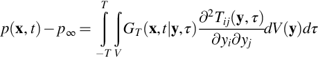
Scattering of turbulent surface pressure fluctuations into sound is one of the dominant mechanisms behind some important aeroacoustic noise sources, such as trailing edge noise and rough-wall boundary layer noise. To relate the surface pressure fluctuations on a flat surface below a turbulent boundary layer to the velocity fluctuations in the boundary layer we can use Lighthill's analogy, provided that the flow is of sufficiently low Mach number that it may be regarded as locally incompressible. Since the distances between the local velocity fluctuations and a point on the surface are small compared to the acoustic wavelength, we need not be concerned with the effect of propagation time on the solution to Lighthill's wave equation given by Eq. (4.3.3). The unsteady surface pressure will be given by ![]() and, since the surface is rigid, the pressure gradient will be zero normal to the surface. We can then replace the Green's function in Eq. (4.3.3) with the tailored Green's function specified in Eq. (4.5.3) to eliminate the surface integral, and give the surface pressure on the surface as
and, since the surface is rigid, the pressure gradient will be zero normal to the surface. We can then replace the Green's function in Eq. (4.3.3) with the tailored Green's function specified in Eq. (4.5.3) to eliminate the surface integral, and give the surface pressure on the surface as
This simplifies considerably if we assume a completely incompressible flow because we can approximate Tij by ρovivj (Section 4.2.1) and the tailored Green's function, for a point on the surface as GT=δ(τ−t)/2π|x–y|, since the distance from the sources and their images to the surface is the same. These approximations are valid very close to the source where the fluctuations are dominated by the hydrodynamic part of the flow and the acoustic waves can be ignored because they are of a completely different scale. Using these approximations and carrying out the integral over time gives
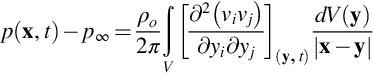
where the terms in square brackets are evaluated at y and t. The mean flow speed in the boundary layer varies with height and so we can split the velocity into its mean and unsteady parts as vi=Ui+ui and so vivj=(UiUj+Uiuj+uiUj+uiuj). It follows then that this formulation gives both a steady and unsteady surface pressure. The unsteady part of the surface pressure is obtained by subtracting the mean of the fluctuations and gives the nonlinear velocity term in Eq. (9.2.23) as
Then making use of the relationship for an incompressible flow that was used in Eq. (4.2.2), we find that, if the mean flow speed is parallel to the boundary in the y1 direction, then

Using these results in Eq. (9.2.23) then gives

The two terms of the integrand are referred to as the rapid and the slow term, respectively. The “rapid” term incorporates the mean-velocity gradient and this is thought of as responding immediately to changes in the mean flow, whereas the “slow” term responds only indirectly as a consequence of the influence of the mean flow on the turbulence structure. The rapid term is often assumed to dominate in boundary layers, and thus is the usual focus of modeling, though DNS calculations show both contributions to be of similar magnitude [25]. In free turbulent flows, where mean-velocity gradients are small, the slow term dominates [26].
At a fundamental level, Eq. (9.2.24) shows that the pressure fluctuation at a point on the wall x=(x1,0,x3) will be given by the integral of fluctuating velocities over the boundary layer, weighted by the inverse of the distance from that point. Thus the pressure fluctuation will tend to reflect contributions from small scale turbulent motions just above the wall as well as from larger scale motions from the outer part of the boundary layer that are coherent over a substantial volume of the flow. Scale decompositions of the pressure fluctuation into frequency or wavenumber-frequency spectra therefore reveal these different contributions.
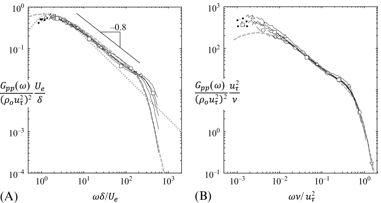
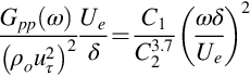
Fig. 9.20 shows the wall-pressure frequency spectrum Gpp(ω) measured under a flat plate turbulent boundary layer flow as a function of momentum-thickness Reynolds number Reθ. At low frequencies pressure fluctuations are predominantly generated by the large structures in the outer part of the boundary layer with scales on the order of the boundary layer thickness δ. The pressure fluctuations generated by these structures should scale on the velocity difference with the free stream that sustains them and thus, consistent with the law of the wake, should scale on ρouτ2. At the same time they are carried over the wall at a convection velocity that will likely be proportional to the edge velocity Ue (Fig. 9.19) and so their passage frequency will scale on Ue/δ. Thus we expect the spectrum in this region to have a fixed form when plotted as:
 , Goody [27];
  , Howe [37].

As demonstrated in Fig. 9.20A we see exactly this behavior, with pressure spectra measured over a 3:1 range of Reynolds numbers grouping into a narrow band that, in this case, extends up to ![]() . Note that there are a number of (mostly minor) variations of the outer scaling that are commonly used, such as using δ⁎ as the distance scale, or assuming a convective velocity scaled on uτ.
. Note that there are a number of (mostly minor) variations of the outer scaling that are commonly used, such as using δ⁎ as the distance scale, or assuming a convective velocity scaled on uτ.
The small near-wall eddies contributing to the pressure spectrum at high frequencies will have sizes determined by the same viscous scale ν/uτ that determines the mean-velocity profile at the bottom of the boundary layer. These structures will be moving at flow-speeds that vary with uτ and produce turbulent velocity fluctuations that scale with uτ and thus, presumably, produce pressure fluctuations that scale as ρout2. The high frequency part of the spectrum should therefore appear invariant when normalized as:
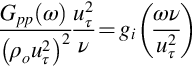
Again this behavior is realized, as illustrated in Fig. 9.20B. It also appears from Fig. 9.20 that there is a mid-frequency range where both the above scalings exist simultaneously. In that case we must have that
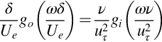
This is only possible if

and thus we expect the pressure spectrum to have a −1 slope in the overlap region when plotted on a log-log scale. Mysteriously almost all turbulent boundary layer experiments, like that represented in Fig. 9.20 reveal a mid-frequency region with a slope of −0.7 to −0.8. A −1 region has been seen in atmospheric boundary layer measurements [29], a finding that may indicate that this behavior may be very slow to appear with increase in Reynolds number.
Analysis [30,31] of the fundamental constraints on the pressure spectrum and of the turbulent contributions to the integrand of Eq. (9.2.24), as well as measurements [32,33] have established other power-law regions in the wall-pressure time spectrum, including a (ωδ/Ue)2 region at low frequencies, and a ![]() region at very high frequencies where the pressure fluctuations are generated by action in the viscous sublayer.
region at very high frequencies where the pressure fluctuations are generated by action in the viscous sublayer.
An empirical interpolation formula for the wall-pressure frequency spectrum, which takes advantage of these scaling regions, was developed by Goody [27] and has the form:
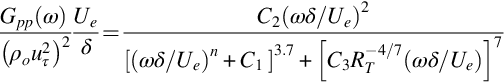
where RT is the ratio of the outer to inner layer timescales (δ/Ue)/(ν/uτ2). Goody recommends the constants:
Goody's equation reduces at low frequencies ![]() to
to
and at high frequencies ![]() to
to

If RT is sufficiently large then a mid-frequency “overlap” range will exist where

Goody chose ![]() based on comparisons with lower-Reynolds number boundary layer measurements than those of Fig. 9.20 where the overlap region slope was observed to be about −0.7. Note that RT was not sufficient in those cases to realize the full implied slope in the overlap region of −0.775. Choosing
based on comparisons with lower-Reynolds number boundary layer measurements than those of Fig. 9.20 where the overlap region slope was observed to be about −0.7. Note that RT was not sufficient in those cases to realize the full implied slope in the overlap region of −0.775. Choosing ![]() agrees very well with the higher Reynolds number, higher slope, and data of Fig. 9.20 and also comes close to satisfying the infinite Reynolds number limit that requires the overlap region slope of −1 predicted by dimensional analysis. The important take-away here is the need for adjustment of the parameter n according to Reynolds number if accuracy in the mid-frequency range is important.
agrees very well with the higher Reynolds number, higher slope, and data of Fig. 9.20 and also comes close to satisfying the infinite Reynolds number limit that requires the overlap region slope of −1 predicted by dimensional analysis. The important take-away here is the need for adjustment of the parameter n according to Reynolds number if accuracy in the mid-frequency range is important.
The full wavenumber-frequency spectrum of surface pressure fluctuations Φpp(k1,k3,ω), as defined in Eq. (8.4.35), is of particular interest for aeroacoustic calculations. This spectrum captures the spatial scales on which the pressure fluctuations occur at each frequency and thus is the source term in surface and trailing edge noise applications. It also captures convection of turbulence over the wall at Uc and thus includes a convective ridge that lies along ![]() . Because of its importance, considerable effort has gone into developing models for the wavenumber-frequency spectrum. We include here the details of a sophisticated model developed by Chase [28] and a more elemental model due to Corcos [34] with the intent that these span the range of need from accuracy to analytical simplicity. A number of other such models have been proposed which may be more easily applied in certain situations, many of which are reviewed by Graham [35], Liu and Dowling [36], and Howe [37]. The Chase model spectrum, in the incompressible limit, is given by the expression:
. Because of its importance, considerable effort has gone into developing models for the wavenumber-frequency spectrum. We include here the details of a sophisticated model developed by Chase [28] and a more elemental model due to Corcos [34] with the intent that these span the range of need from accuracy to analytical simplicity. A number of other such models have been proposed which may be more easily applied in certain situations, many of which are reviewed by Graham [35], Liu and Dowling [36], and Howe [37]. The Chase model spectrum, in the incompressible limit, is given by the expression:
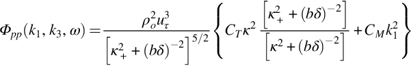
where κ is the magnitude of the in-plane wavenumber vector ![]() , and
, and ![]() is κ modified according to the difference of k1 and its value on the convective ridge, ω/Uc, normalized on a multiple h of the friction velocity, so
is κ modified according to the difference of k1 and its value on the convective ridge, ω/Uc, normalized on a multiple h of the friction velocity, so

Chase recommended that the empirical constants take the values
and the range of validity is Ue/co≪1, κ≫|ω|/co, and ωδ/Ue>1.
Fig. 9.21 shows a perspective view of the Chase spectrum in wavenumber frequency space which forms a thin tongue aligned with the convective ridge. The spectrum extends further in spanwise wavenumber (k3) than streamwise (k1) because the boundary layer turbulence correlates over significantly greater distances in the streamwise than spanwise direction. The exact frequency spectrum corresponding to Eq. (9.2.34) can be derived [35], but a simpler, approximate form due to Chase [31] and given by Howe [37] is,


This spectral form is compared with data and Goody's model in Fig. 9.20A. We see that the Chase model includes no viscous range at high frequencies, and at mid-frequencies takes on the − 1 slope expected at very high Reynolds number.
The Corcos spectrum provides an algebraically simpler wavenumber-frequency spectrum model with the form
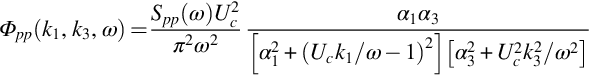
with empirical constants ![]() and
and ![]() . Note that Corcos' formulation leaves the frequency spectrum Spp(ω) unspecified.
. Note that Corcos' formulation leaves the frequency spectrum Spp(ω) unspecified.