
Leading edge noise
Abstract
One of the most important noise sources in low Mach number flows is the result of a blade moving through a region of unsteady flow or turbulence. The mechanism that causes the sound that radiates to the acoustic far field is referred to as leading edge noise. There are many examples where this sound source occurs including fans of all types, helicopter rotors and propellers. This chapter discusses the mechanisms of leading edge noise and shows how it can be calculated for a stationary blade in a uniform flow.
Keywords
Compressible blade response function; Sub and supercritical waves; Arbitrary gust response; Blade vortex interaction; Turbulence ingestion noise
One of the most important noise sources in low Mach number flows is a blade moving through a region of unsteady flow or turbulence. The sound that radiates to the acoustic far field is referred to as leading edge noise. There are many examples where this sound source occurs including fans of all types, helicopter rotors and propellers. This chapter discusses the mechanisms of leading edge noise and shows how it can be calculated for a stationary blade in a uniform flow.
14.1 The compressible flow blade response function
In Chapter 6 we introduced thin airfoil theory and showed how the unsteady flow over a thin blade could be approximated to first order by considering the same flow over an infinitely thin flat plate at zero angle of attack, as shown in Fig. 6.7. This approximation is valid providing that the mean flow speed around the blade does not differ from the free stream flow speed U∞ by more than ±ɛU∞ and the amplitude of the unsteady gust is also of order ɛU∞, where ɛ≪1 is a small parameter. We then considered the case of an acoustically compact stationary blade in an incompressible mean flow and showed that the source of sound was equivalent to an acoustic dipole with its axis normal to the flow, and strength equal to the net unsteady force produced by the blade. The relationship between the unsteady force and the amplitude of a harmonic incident gust was given by Sears function and was critically dependent on the application of the Kutta condition at the blade trailing edge since this controls the circulation about the blade. However, in aeroacoustic applications we are also concerned with compressible flows, and the modeling of the unsteady loading by an incompressible flow approximation is a severe limitation. We must therefore investigate in detail the effects of compressibility on the blade response function so that the limitations of incompressible flow theory are well defined.
14.1.1 The compressible and incompressible flow blade response to a step gust
If a step upwash gust is swept past a stationary blade, then there will be a sudden change in angle of attack that convects across the blade surface. In an incompressible flow the whole flow reacts instantaneously to any change in boundary conditions, and so when the gust strikes the leading edge of the blade vorticity is shed into the blade wake at the same instant in order to satisfy the Kutta condition at the trailing edge. In a compressible fluid the physical mechanism is quite different. In general, information propagates through the medium at the speed of sound, and so the trailing edge boundary condition will be unaltered until the acoustic wave generated at the leading edge by the gust interaction reaches the trailing edge. Since the wave propagation speed is enhanced by the mean flow convection the time taken for the acoustic wave to travel from the leading edge to the trailing edge is c/(c∞+U∞), where c is the blade chord, U∞ is the mean flow speed, and c∞ is the speed of sound. To determine if this delay is important we must consider the phase shift between the leading edge pressure fluctuations and the trailing edge pressure. If the frequency of interest is ω then the phase shift will be ωc/(c∞+U∞). For incompressible flow c∞ is infinite, and so the phase shift is zero. A step gust however excites all frequencies, and so an incompressible flow calculation of the unsteady loading from a step gust will only be valid for the low frequency part of the loading spectrum.
We can write this criterion in terms of the acoustic wavenumber k=ω/c∞ and the Mach number M=U∞/c∞ and require that
for incompressible flow theory to be valid. This is the same as requiring that the blade chord be acoustically compact, which was the assumption used in Section 6.4. However, in many applications this requirement is not met. For example, a frequency of 1000 Hz and a blade chord of 30 cm imply kc=5.5 in air, and so the incompressible flow assumption is far from valid. In underwater applications with the same dimensions and at the same frequency kc=1.25, and so compressibility effects are also important even though the medium is almost incompressible.
An alternative perspective is obtained if the incoming gust has a streamwise scale Lw, so the peak frequency excited by the gust is ω=2πU∞/Lw. The criterion given by Eq. (14.1.1) then becomes
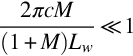
Since the lengthscale of the gust is likely to be of the same magnitude as the blade chord, the criterion is primarily determined by the flow Mach number M. The Mach number for a π/2 phase shift is then M=0.333, and at flow speeds substantially less than this the incompressible flow approximation is valid. However, some caution needs to be used in extending this concept to frequencies that are well above the peak frequency of the incoming gust and lie in the range where kc is of order one, and this can occur if the lengthscale of the incident turbulence is much smaller than the blade chord.
14.1.2 Leading and trailing edge solutions
In most aeroacoustics applications the Mach number is usually 0.3 or greater, and the frequencies of interest are 500 Hz and above, so the effect of compressible flow on the blade response function cannot be ignored. Unfortunately, there is no complete analytical solution to the flat plate blade response function in a compressible flow, and numerical methods have to be used for the full calculation. However, there are close approximations to the solution based on an iterative approach proposed by Landahl [1]. In the first iteration the blade is assumed to be a semi-infinite flat plate, as shown in Fig. 13.5. This will give a solution that satisfies the boundary conditions on the plate and in the upstream flow, but it also causes a pressure jump across the wake that does not satisfy the Kutta condition. To ensure a zero pressure jump across the wake a second solution is added to the first solution that exactly cancels the pressure jump across the wake but induces no additional upwash upstream of the trailing edge. This second solution is found by solving a semi-infinite plate trailing edge problem as shown in Fig. 13.1. The sum of the two solutions satisfies the blade boundary conditions and the Kutta condition but induces a pressure discontinuity upstream of the leading edge. To correct this a third solution is added which eliminates the upstream pressure jump and satisfies the nonpenetration boundary condition on the blade surface but induces a pressure jump over the wake which needs to be corrected. This process can be repeated indefinitely and converges to a solution if the residual pressure jumps in the wake become smaller and smaller. Fortunately, the convergence is quite quick at high frequencies, and usually only the first two terms in the series are needed to achieve acceptable results.
14.1.3 The first-order solution for the surface pressure
The first-order solution can be obtained using the Weiner–Hopf method as described in Section 13.4. The unsteady pressure jump across a blade, modeled by a semi-infinite flat plate, caused by a harmonic upwash gust of amplitude ![]() , as shown in Fig. 13.5, was given by Eq. (13.4.5) and is repeated here as
, as shown in Fig. 13.5, was given by Eq. (13.4.5) and is repeated here as
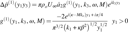
where positions have been written in terms of coordinate y, and we have explicitly included the time dependency. The origin of y is at the leading edge. For a gust convected by the mean flow the wavenumbers are given by
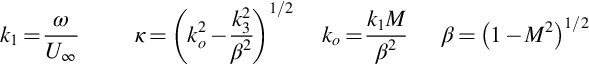
The first point to note from this result is that the surface pressure tends to infinity as y1−1/2 at the leading edge of the blade. This behavior is expected from the steady flow around an airfoil at a small angle of attack and is the result of the flat plate approximation. If the airfoil had a rounded leading edge then the pressure would remain finite as y1 tends to zero. Next consider the phase which depends on (κ−Mko)y1+k3y3 and indicates a wave propagating in the positive y1 and y3 directions, assuming that k1>0 and k3>0. If k3=0 then the phase reduces to
which represents a wave propagating downstream at the speed of sound plus the free stream speed, as discussed earlier. The surface pressure is therefore controlled by an acoustic wave propagating over the surface downstream from the leading edge.
If k3 is given a value in the range 0<k3<βko then we can write k3=βkosinφ and κ=kocosφ. The phase variation in Eq. (13.4.5) then represents an acoustic wave propagating at an angle to the y1 direction defined by

as shown in Fig. 14.1A, for example, for M=0.3, φ=π/8 radians, giving φe=30.3 degrees.

Because this is an acoustic wave it will couple strongly with the acoustic far field, and there will be radiation in the direction of φe. This is referred to as a super-critical wave [2]. In contrast for the case when |k3|>βko we find from Eq. (14.1.3) that κ is a positive imaginary number (because of the choice of the branch cut), and the wave decays exponentially in the y1 direction. This is referred to as an evanescent or subcritical wave and is illustrated in Fig. 14.1B. Because this wave does not propagate it will not radiate to the acoustic far field.
Turbulent flows that are dominated by eddies with small lengthscales in the spanwise direction will contain significant energy at wavenumbers where k3 is subcritical. The fluctuations at these wavenumbers will have little impact on the acoustic far field because they do not couple with the acoustic wavenumbers that radiate sound. However, evanescent waves can dominate the pressure fluctuations measured on the surface close to the leading edge. Consequently, trying to relate measured pressure fluctuations on the blade surface near the leading edge to the far-field sound is not straightforward. Eq. (13.4.5) shows that at high spanwise wavenumbers |k3|≫βko and the surface pressure fluctuations caused by subcritical waves will decay with distance from the leading edge as ![]() . So, the unsteady pressure caused by the gust may be quite local to the leading edge, and its initial decay may be much faster than would be expected if the evanescent wave was not considered. However, because of this rapid decay, the surface pressure should asymptote to the super-critical case for surface pressures measured more than an acoustic wavelength downstream of the leading edge.
. So, the unsteady pressure caused by the gust may be quite local to the leading edge, and its initial decay may be much faster than would be expected if the evanescent wave was not considered. However, because of this rapid decay, the surface pressure should asymptote to the super-critical case for surface pressures measured more than an acoustic wavelength downstream of the leading edge.
An alternative interpretation of this effect is obtained if we consider the speed with which the intersection between the gust wavefront and the leading edge propagates along the blade in the spanwise direction. Since the gust wavelength in the spanwise direction is 2π/k3 and the gust period experienced at the leading edge is 2π/ω, this speed is ci=ω/k3. For this wave to be supercritical we require that |k3|<βko=ω/βc∞ or ω/β|k3|c∞>1, and it follows that we require |ci|/βc∞>1. The wavefront must therefore propagate across the surface in the spanwise direction at a speed that is greater than the speed of sound.
The first-order solution for the surface pressure given above is for a semi-infinite flat plate and can be corrected to allow for finite chord using the approach given in Section 13.6. The correction is obtained by adding a solution to the boundary value problem that ensures that there is no pressure jump across the wake of the blade that extends downstream from y1=c while maintaining zero velocity normal to the blade surface for y1<c. The correction discussed in Section 13.4 is only a first-order approximation to the complete solution because the surface pressure induced by the leading edge is assumed to be a simply convected wave with no decay with distance downstream. Given this approximation the blade response function with the trailing edge correction is given by Eq. (13.4.6) as
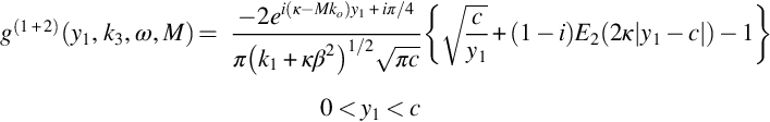
where, as above, positions have been written in terms of the coordinate y1. The additional correction includes the complex Fresnel integral defined as
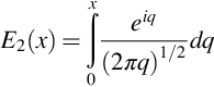
which is shown in Fig. 14.2.

For large arguments the complex Fresnel integral has the asymptotic value of (1+i)/2, so the last two terms of Eq. (13.4.6) cancel as 2κ|y1−c| tends to infinity. It follows therefore that at high frequencies the trailing edge correction causes a small oscillation of the pressure about first-order solution for positions significantly upstream of the trailing edge and ensures the pressure is zero at the trailing edge as illustrated in Fig. 14.3. Most of the physics of the problem can therefore be obtained from the first-order solution, and at high frequencies, the combined first- and second-order solution is well approximated by the first-order solution if it is truncated at the trailing edge of the blade.

14.1.4 The unsteady lift in compressible flow
The blade response function also gives the total lift on the blade surface caused by the upwash gust, and this can be obtained from Eq. (13.4.7) by integrating the pressure over both the blade span and the blade chord. For blades with large span the spanwise integral will be zero if k3≠0 because of the oscillatory nature of Δp with y3, and so the loading depends only on the amplitude of the gust with zero spanwise wavenumber. Integrating Eq. (13.4.6) is complicated by the trailing edge correction, but, as discussed earlier, this will have a small effect on the result at high frequencies. A good approximation is obtained by integrating the first-order solution given by Eq. (13.4.5). We then obtain the nondimensional unsteady lift per unit span, normalized by ![]() as in Eq. (6.4.4), as
as in Eq. (6.4.4), as
where the reduced frequency σ=ωa/U∞ and a=c/2 is the semi-chord. The negative sign is because Δp represents the pressure on the top of the airfoil less that on the bottom. This integral can be evaluated directly to give
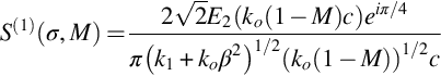
This is often written in terms of the nondimensional variables
which gives (after using (1+i)=√2exp(iπ/4))

In the high frequency limit the function E2(x) will asymptote to (1+i)/2, and so we can approximate

where we have used the relationship ![]() . This shows that the first-order approximation to the compressible blade response function is inversely proportional to the nondimensional frequency at high frequencies. This scaling is quite different from the incompressible results given by Sears function (Eqs. 6.4.4, 6.4.5) that scaled inversely with the square root of the nondimensional frequency. The compressibility effect is therefore to reduce the high-frequency response of the blade, and this has an increasingly important effect in high speed flows. Fig. 14.4 illustrates this difference for a flow Mach number of M=0.3. At low frequencies the magnitude of the compressible solution is slightly larger than the incompressible solution, but this is caused by the approximate nature of the compressible solution which only includes the first-order approximation without the trailing edge or additional leading edge corrections. However, at high frequencies, where the first-order compressible blade response function is a more accurate approximation, the incompressible and compressible solutions are very different. Amiet [3] notes that the incompressible solution is appropriate to use when σM/β2<π/4, which corresponds to the frequency where the blade chord (divided by β2) is less than a quarter of the acoustic wavelength. For the example shown in Fig. 14.4 the compressible blade response function should be used at nondimensional frequencies σ>2.38 according to Amiet's criterion, as shown by the vertical line in the figure. This corresponds to the lowest frequency where the compressible blade response is less than the incompressible response.
. This shows that the first-order approximation to the compressible blade response function is inversely proportional to the nondimensional frequency at high frequencies. This scaling is quite different from the incompressible results given by Sears function (Eqs. 6.4.4, 6.4.5) that scaled inversely with the square root of the nondimensional frequency. The compressibility effect is therefore to reduce the high-frequency response of the blade, and this has an increasingly important effect in high speed flows. Fig. 14.4 illustrates this difference for a flow Mach number of M=0.3. At low frequencies the magnitude of the compressible solution is slightly larger than the incompressible solution, but this is caused by the approximate nature of the compressible solution which only includes the first-order approximation without the trailing edge or additional leading edge corrections. However, at high frequencies, where the first-order compressible blade response function is a more accurate approximation, the incompressible and compressible solutions are very different. Amiet [3] notes that the incompressible solution is appropriate to use when σM/β2<π/4, which corresponds to the frequency where the blade chord (divided by β2) is less than a quarter of the acoustic wavelength. For the example shown in Fig. 14.4 the compressible blade response function should be used at nondimensional frequencies σ>2.38 according to Amiet's criterion, as shown by the vertical line in the figure. This corresponds to the lowest frequency where the compressible blade response is less than the incompressible response.

14.1.5 An arbitrary gust
The results given so far in this section have been for a harmonic gust with space dependence ![]() in the plane of the blade, y2=0. To extend these results to an arbitrary gust we consider the upwash velocity on the blade surface y2=0 to be the superposition of gusts with a spectrum of wavenumbers, so
in the plane of the blade, y2=0. To extend these results to an arbitrary gust we consider the upwash velocity on the blade surface y2=0 to be the superposition of gusts with a spectrum of wavenumbers, so

The pressure jump across the blade is then obtained by superimposing the contributions from each wavenumber component of the gust, so using Eq. (13.4.5) with g(1+2) from Eq. (13.4.6), and substituting ![]() for â2, including the time dependence that is suppressed in Eq. (13.4.5), we obtain
for â2, including the time dependence that is suppressed in Eq. (13.4.5), we obtain

The Fourier transform of this signal with respect to time is obtained by replacing k1 by ω/U∞, and so the integrand over k1 in Eq. (14.1.8) is simply an inverse Fourier transform with respect to time, as defined in Eq. (3.10.2), and so

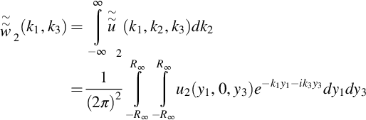
Further simplification is possible if we note that the gust response is independent of the k2 wavenumber, so we have

where ![]() is the planar wavenumber transform of u2(y1, 0, y3) in the plane y2=0, so
is the planar wavenumber transform of u2(y1, 0, y3) in the plane y2=0, so
These results give the unsteady loading on a blade encountering an arbitrary gust. It is important to note that there are some subtle differences between the results for a harmonic gust given by Eq. (13.4.5) and the frequency domain result given by Eq. (14.1.10). The spanwise dependence of the general gust is completely determined by the wavenumber integral defined in Eq. (14.1.11), and so any spanwise dependence can be included. For example, if the gust is of finite spanwise extent then this characteristic will appear as part of the wavenumber spectrum as a function of k3.
14.2 The acoustic far field
14.2.1 The acoustic far field from the leading edge interaction
The acoustic field that results from unsteady pressure fluctuations on a thin plate in uniform flow is given by Eq. (6.5.5), as

In obtaining this result we made use of Prantl-Glauert coordinates and the far-field approximation, so the blade chord c and span b=2d are required to be small compared to the propagation distance re.
It will be convenient, when we come to rotor noise calculations in Chapter 16, to have this result expressed in terms of the acoustic pressure perturbation pʹ=ρʹc∞2 and the wavenumber transform of the surface pressure, as given by Eqs. (4.7.12) and (6.5.6),
and

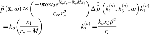
The important feature of this result is that ![]() has dimensions of a force (per unit frequency, per unit wavenumber squared) and so, in the limit that ko is very small,
has dimensions of a force (per unit frequency, per unit wavenumber squared) and so, in the limit that ko is very small, ![]() , and Eq. (14.2.1) reduces to a dipole source that depends on the force produced by the blade. However, when the acoustic wavelength is comparable to the blade span or chord then the unsteady loading on the blade surface couples to the acoustic field at the wavenumbers k1(o) and k3(o). To obtain the far-field sound,
, and Eq. (14.2.1) reduces to a dipole source that depends on the force produced by the blade. However, when the acoustic wavelength is comparable to the blade span or chord then the unsteady loading on the blade surface couples to the acoustic field at the wavenumbers k1(o) and k3(o). To obtain the far-field sound, ![]() must therefore be evaluated at the appropriate wavenumbers which will depend on the observer location. A special case is for semi-infinite blade chord because in that case the blade chord is always large compared to the wavelength, and so the directionality will be distinctly different from the case of a blade with an acoustically compact chord.
must therefore be evaluated at the appropriate wavenumbers which will depend on the observer location. A special case is for semi-infinite blade chord because in that case the blade chord is always large compared to the wavelength, and so the directionality will be distinctly different from the case of a blade with an acoustically compact chord.
In order to obtain the wavenumber transform of the surface pressure we use Eq. (14.1.10) in Eq. (4.7.12). First consider the integral over the span. In Eq. (14.1.10) the dependence on span is given by an inverse Fourier transform over k3, whereas Eq. (4.7.12) evaluates a forward transform as a function of y3. It follows that the integrand in Eq. (14.1.10) matches the forward transform in Eq. (4.7.12). Given this observation we obtain
where the integral over the chord is specified by

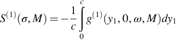
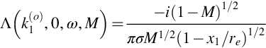
The function Λ defined in Eq. (14.2.3) is closely related to the nondimensional lift on the airfoil surface. Since this is accurately represented by the first-order approximation to the unsteady surface pressure response we can simplify the evaluation of Eq. (14.2.3) by using g(1) instead of g(1+2). The function Λ can then be interpreted as the nondimensional blade response function as observed in the acoustic far field and can be evaluated directly from Eq. (13.4.5) as

providing that κ (evaluated here using k3(o)) is real and κ>kox1/re. This condition is always met when the spanwise wavenumber of the incident gust is zero, but some care must be taken when evaluating this result for larger spanwise wavenumbers particularly where the observer is near the x1 axis.
14.2.2 The far-field directionality and scaling
To provide some insight into the scaling in the acoustic far field we consider the case when the observer is in the plane x3=0, and so spanwise gust wavenumber is zero ![]() . In this case κ=ko=ωM/U∞β2, and we obtain
. In this case κ=ko=ωM/U∞β2, and we obtain

In the high-frequency limit the Fresnel function tends to (1+i)/2, and we obtain
An important feature of this result is that it provides the scaling of the far-field sound on the mean flow Mach number.
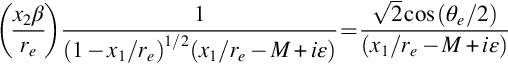
The directionality in the far field is also quite different from the dipole directionality discussed in Chapter 4 for acoustically compact surfaces. Combining Eqs. (14.2.1), (14.2.2), and (14.2.6) shows that the far-field sound depends on

which gives a cardioid-shaped directionality as shown in Fig. 14.5A and is quite different from the dipole directivity given by sinθe shown in Fig. 14.5B. However, if the effect of finite chord is included and the directionality is calculated by using Eq. (14.2.5), the directionality has multiple lobes and a null in the upstream and downstream directions similar to that of a dipole (see Fig. 14.5C and D).

14.2.3 Impulsive gusts of finite span
Further insight is obtained by considering an impulsive gust of very short duration that is constant over a finite span b. The impulsive gust can be characterized by a Dirac delta function scaled on the blade semi-chord in the direction of the flow, and so the upwash is
In this case we find that the wavenumber transform in Eq. (14.1.11) reduces to
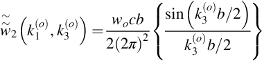
When this result is used in Eq. (14.2.2) to calculate the acoustic far field it is seen that the directionality in the y3 direction is determined by the terms in {}. If the spanwise extent of the gust is large then the directionality will have a clearly defined beam of sound that is strongest in the direction where ![]() . The sound radiation is therefore primarily in the direction normal to the plane of the blade where x3=0. However, when the spanwise extent of the gust is much smaller than the acoustic wavelength then kob≪1, and the terms in {} are approximately unity for all observer angles, so the directionality in both the x1 and x3 direction is determined by x2Λ/re and is independent of the gust. This is important in cases where the spanwise correlation lengthscale of a gust is small because in that case the directionality is determined entirely by the acoustics and the blade response function.
. The sound radiation is therefore primarily in the direction normal to the plane of the blade where x3=0. However, when the spanwise extent of the gust is much smaller than the acoustic wavelength then kob≪1, and the terms in {} are approximately unity for all observer angles, so the directionality in both the x1 and x3 direction is determined by x2Λ/re and is independent of the gust. This is important in cases where the spanwise correlation lengthscale of a gust is small because in that case the directionality is determined entirely by the acoustics and the blade response function.
14.2.4 A step gust
A similar important example is given by a step gust for which
Ahead of the gust the upwash velocity is zero, and behind the gust the upwash is wo. Providing that spanwise extent of the gust is much smaller than the acoustic wavelength we obtain using Eq. (14.1.11)

where a small imaginary part has been added to the wavenumber to ensure the wavenumber transform converges. The difference between the step upwash gust and the impulsive gust is that the step gust is inversely proportional to the wavenumber ![]() , and this will alter the far-field directionality and the spectral shape. At high frequencies and for an observer at x3=0 we can use Eqns. (14.2.1), (14.2.2), and (14.2.7) to give the directionality for a step gust as
, and this will alter the far-field directionality and the spectral shape. At high frequencies and for an observer at x3=0 we can use Eqns. (14.2.1), (14.2.2), and (14.2.7) to give the directionality for a step gust as
The interesting characteristic of this result is that for a step gust there will be a strong beam of radiation at the angle where x1/re=M, which is caused by the sudden change in the unsteady lift. This is a characteristic of the step gust, specifically its permanent change in the angle of attack of the mean flow.
14.3 An airfoil in a turbulent stream
One of the most important applications of leading edge noise is to blades embedded in a turbulent flow. While these flows are usually inhomogeneous, they can often be modeled by a homogeneous turbulent flow with the same characteristics, such as turbulence intensity and lengthscale. To determine the characteristics of the radiated sound we will combine the results obtained above with the models of homogeneous turbulence discussed in Section 9.1, to obtain an estimate of the power spectrum of the far-field noise.
The power spectrum of a signal can be obtained from its Fourier transform using Eq. (8.4.13), and so if we consider a blade of large span we can use Eqs. (14.2.1) and (14.2.2) to define the far-field spectral density of the acoustic pressure as
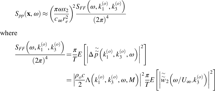
and T is half the averaging time used to obtain the spectral estimate. The term SFF(ω,k1(o),k3(o)) represents the spectrum of the unsteady force produced by the airfoil that couples with the acoustic field that radiates to an observer at x. At low frequencies when the blade is acoustically compact it is simply the unsteady loading spectrum on the blade. However, at high frequencies it will depend on the observer location x as well as the flow Mach number.
This result is still quite general and applies to both a homogeneous and an inhomogeneous flow providing that we can define the expected value of the turbulence spectrum. We can use Eq. (8.4.38) written as
and thus,

where ϕ22 is the planar wavenumber spectrum and can be defined using Eqs. (9.1.14) or (9.1.23), using different empirical models for the turbulent spectrum. The averaging time T is defined by the time it takes the volume of turbulence to pass over the blade, and so R∞/T=U∞. In this result the size of the turbulent region also determines the wetted span of the blade, and so R∞=b/2. We then obtain the effective loading spectrum as

A suitable model for the planar wavenumber spectrum is given by the von Kármán turbulence model and is defined by Eq. (9.1.14) as

The scaling of the far-field sound is revealed by using the approximation given by Eq. (14.2.6) for an observer in the y3=0 plane. This gives the far-field pressure as

This reveals that the spectral density scales with the fourth power of the flow speed, since ![]() will scale with
will scale with ![]() , which is a direct consequence of the leading edge scattering mechanism and the fact that the spectral density has been chosen to describe the far field. If a spectral level is measured then it will depend on the bandwidth of the measurement and will be given by ΔωSpp(ω). The right side of the equation is then adjusted by multiplying by
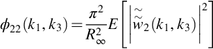
, which is a direct consequence of the leading edge scattering mechanism and the fact that the spectral density has been chosen to describe the far field. If a spectral level is measured then it will depend on the bandwidth of the measurement and will be given by ΔωSpp(ω). The right side of the equation is then adjusted by multiplying by ![]() , and the scaling of the far-field sound will depend on the fifth power of the mean flow speed. This is an important difference from the dipole scaling laws discussed in Chapter 4 that suggest the sound radiation scales on the sixth power of the flow speed and is a direct consequence of the compressibility effects that are controlling the unsteady loading at the leading edge of the blade. Another important feature of this result is that the spectral level ΔωSpp(ω) scales as b/ke~bLf, so it depends on the blade span multiplied by the integral lengthscale of the turbulence. Reducing the integral lengthscale of the turbulence therefore reduces the overall level of the spectrum. However, it also alters the spectral shape. To illustrate this point Fig. 14.6 shows a typical spectrum plotted as a function of the nondimensional frequency for different values of Lf/c. It is seen that the spectrum shifts to the right as the integral length scale is reduced, increasing the high frequency content of the spectrum, but the low-frequency levels are reduced.
, and the scaling of the far-field sound will depend on the fifth power of the mean flow speed. This is an important difference from the dipole scaling laws discussed in Chapter 4 that suggest the sound radiation scales on the sixth power of the flow speed and is a direct consequence of the compressibility effects that are controlling the unsteady loading at the leading edge of the blade. Another important feature of this result is that the spectral level ΔωSpp(ω) scales as b/ke~bLf, so it depends on the blade span multiplied by the integral lengthscale of the turbulence. Reducing the integral lengthscale of the turbulence therefore reduces the overall level of the spectrum. However, it also alters the spectral shape. To illustrate this point Fig. 14.6 shows a typical spectrum plotted as a function of the nondimensional frequency for different values of Lf/c. It is seen that the spectrum shifts to the right as the integral length scale is reduced, increasing the high frequency content of the spectrum, but the low-frequency levels are reduced.
 .
.14.4 Blade vortex interactions in compressible flow
Blade vortex interaction is an important source of sound in situations where a blade tip vortex on a rotor washes over a structure or is re-ingested into the rotor. An example is a helicopter executing a maneuver in which the blade tip vortices are washed back into the rotor plane and are cut by the blades. As a result, a loud thumping sound is heard, and the far-field sound levels can be very high. This topic will be discussed in more detail in Chapter 16, and in this section we describe the approach to calculating the sound from a blade vortex interaction developed by Amiet [4].
In Section 7.5 we discussed the unsteady loading on a blade caused by a passing vortex in incompressible flow. For rotor blades moving with tip speeds (such as a helicopter rotor) that approach the speed of sound the incompressible flow approximation is no longer valid, and so in this section we use the compressible blade response function to calculate the radiated sound. However, the approach is not limited to compressible flows and can also be used at low Mach numbers with the correct adjustment to the blade response function.
14.4.1 The upwash velocity spectrum from a blade vortex interaction
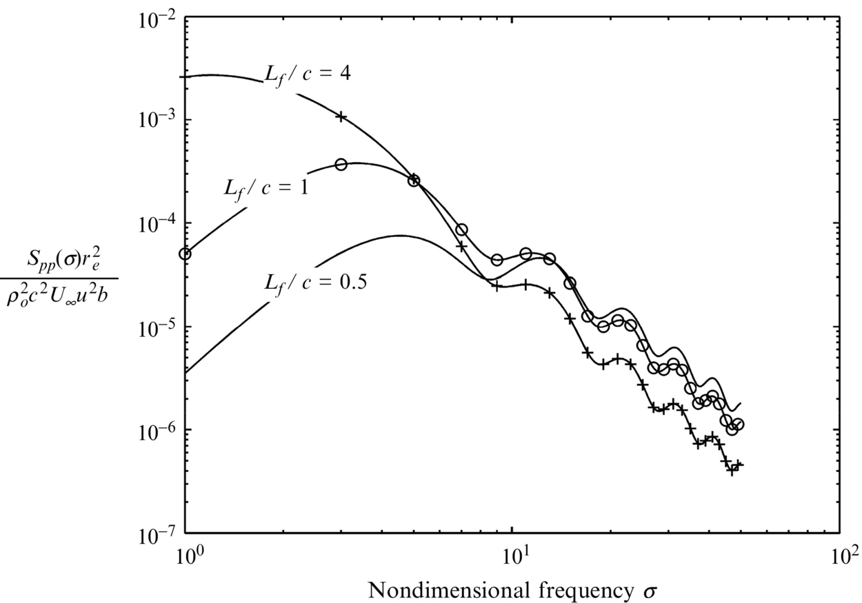
In this section we consider a three-dimensional vortex incident on a stationary blade in a uniform flow, Fig. 14.7. The vortex axis makes an angle ϕv to the leading edge of the blade, as shown. The vortex is convected with the speed U∞ in the y1 direction and, as in Section 7.5, it is a height h above the blade.
We can use the general gust description given by Eq. (14.1.11) to calculate the upwash spectrum that is needed to obtain the acoustic field using Eqs. (14.2.1) and (14.2.2). This is convenient for a flow that is dominated by a line vortex because we can use Eq. (6.3.10) to relate the wavenumber spectrum of the velocity perturbation to the wavenumber spectrum of the vorticity as

For a line vortex the vorticity can be easily expressed using the coordinates (ξ1, ξ2, ξ3), where ξ3 is aligned with the vortex core, that is, in the direction of the unit vector z as shown in Fig. 14.7. Coordinate ξ2 is defined normal to the blade surface. The vorticity is then
In blade-based coordinates yi we have that z=(sinϕv, 0, cosϕv), where ϕv is the angle that the vortex core makes with the blade leading edge, ξ2=y2 and
The wavenumber spectrum of the vorticity is then obtained by integrating over ξ1 and ξ2 and noting that the arguments of the Dirac delta functions are zero when y2=h and ξ1=0, so
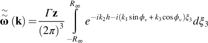
If the vortex is of finite length L then we can take R∞=L/2 and
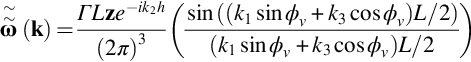
To obtain the upwash spectrum on the blade surface we use Eqs. (14.1.10) and (14.4.1), noting that the component of k×z in the y2 direction is k3sinϕv−k1cosϕv, so
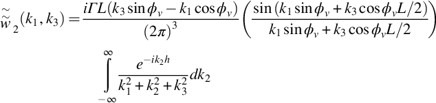
The integral can be completed analytically using tables of Fourier transforms, and we obtain

where ![]() .
.
Based on this result we can calculate the acoustic far field using Eqs. (14.2.1) and (14.2.2), by setting k3=kox3β2/re and k1=ω/U∞. In this case, the argument of the sinc function above becomes
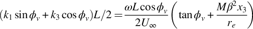
This implies that there will be a strong beam of radiation in the direction where
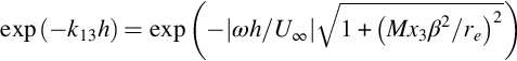
Note that if the angle of the vortex to the leading edge of the blade ϕv is large enough then the right-hand side of this expression will be greater than 1, this beam will not occur, and the peak level of the acoustic field will be greatly reduced. Blade vortex interaction noise is therefore only significant when
which gives a design criterion for this type of source. If the aerodynamics of a rotor can be altered so that the interaction angle meets this criterion, then the loud thumping sound associated with a BVI is avoided.
We also note that the strength of the acoustic field depends on
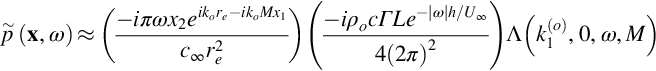
This differs from the two-dimensional result by a factor dependent on M2 and can be ignored for most Mach numbers of interest. The scaling of a blade vortex interaction on frequency will be strongly affected by the displacement of the vortex above the blade, given by h. To illustrate this, consider a parallel interaction at the observer location x3=0 (so ϕv=0 and ![]() ) and use Eq. (14.4.2) in Eqs. (14.2.1) and (14.2.2) to give
) and use Eq. (14.4.2) in Eqs. (14.2.1) and (14.2.2) to give
In the high-frequency limit we can use Eq. (14.2.6) to approximate Λ, and so
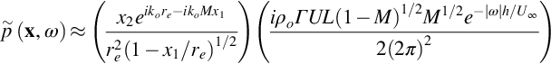
This shows the cardioid directivity expected from a leading edge interaction for blades with noncompact chords and a scaling with flow speed that is much stronger than a traditional unsteady loading source. (Since Γ would be expected to scale on M the Mach number scaling for the mean-square acoustic pressure is approximately M3.) However, the exponential decay of the spectrum with frequency is the dominant effect.