
Open rotor noise
Abstract
Open rotor noise derives from a variety of different sources that can result in tone or broadband noise. In this chapter we discuss these different sources and present analytical methods for the prediction of some of the most important for low Mach number flows. Time and frequency domain approaches to the prediction of loading noise and thickness noise are presented. Amiet's approximation for the prediction of broadband rotor noise is introduced. The chapter concludes with a discussion of the haystacking phenomenon and the prediction of rotor noise when there is significant blade-to-blade correlation.
Keywords
Loading noise; Thickness noise; Time domain methods; Frequency domain methods; Haystacking; Blade-to-blade correlation
Up to this point in the text we have derived the basic equations of aero and hydroacoustics and have presented the analytical methods needed to solve them. We have also considered idealized problems such as leading and trailing edge noise. We will now turn our attention to specific problems that can be addressed using these theories. The first problem we will consider is the noise from propellers and rotors.
16.1 Tone and broadband noise
There are many applications in which rotor noise is a serious problem and a cause for concern. The commercial usage of propeller-driven aircraft is limited by high levels of cabin noise. Ship propellers are a major cause of both shipboard noise and sound radiation to the far field. Airboats are propeller driven and generate high noise levels when running at full speed. On a larger scale, wind turbines can be very noisy if designed incorrectly. Helicopter rotors have many of the same characteristics as propellers, and there are both military and civil applications in which the reduction of helicopter noise is important. In all these examples the same source mechanisms are found, but the dominant processes depend on the application. In this section we discuss the different mechanisms that cause noise from propellers and rotors, and then, in the following sections, we derive prediction methods for each source type.
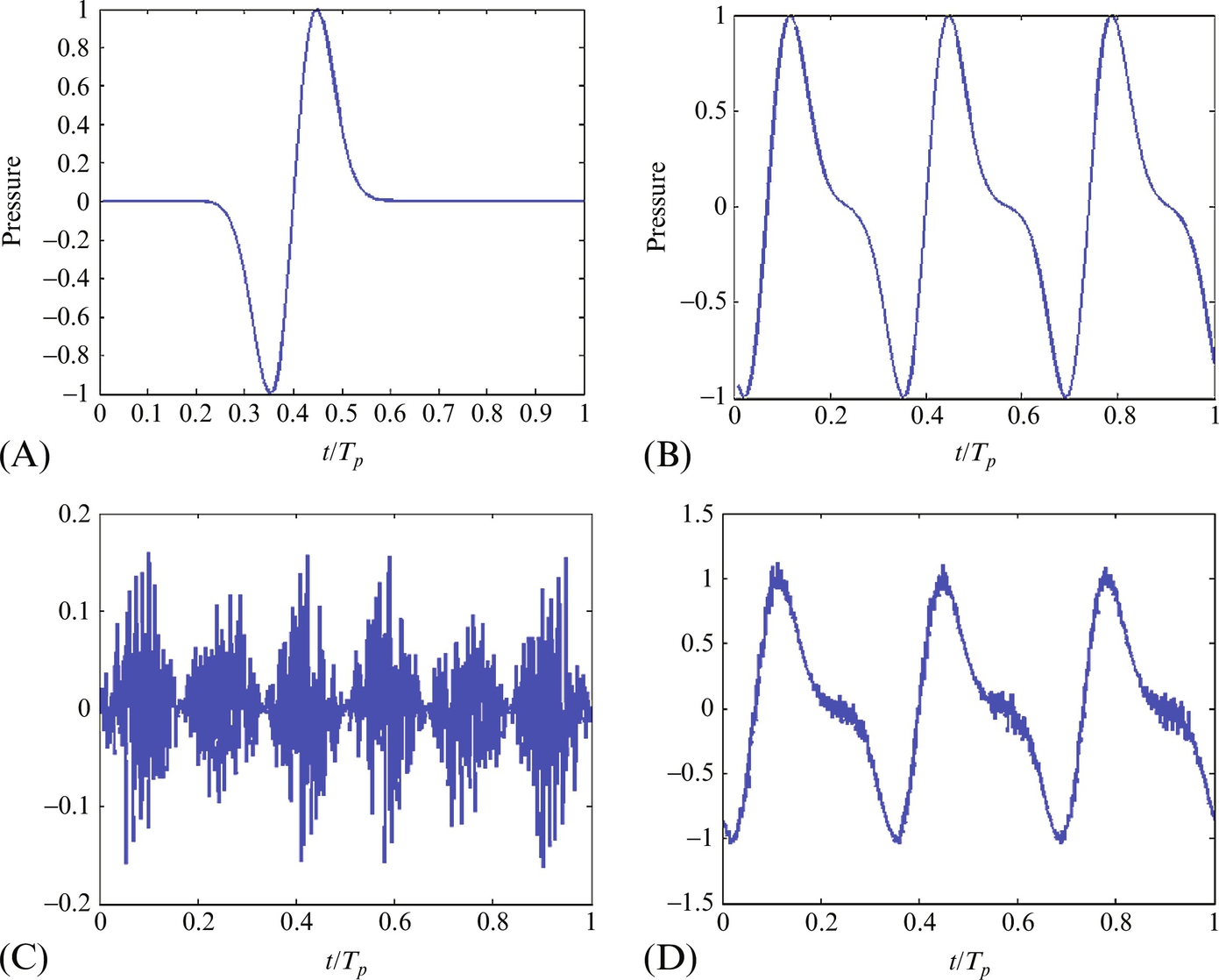
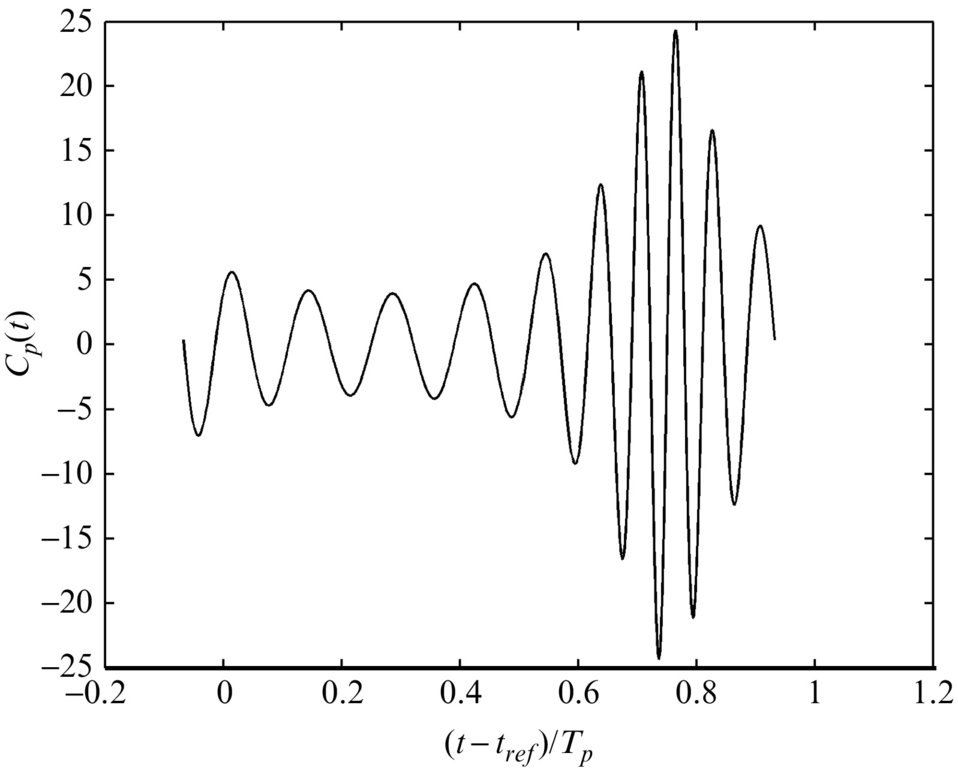
Rotating blades emit two distinctly different types of acoustic signatures. The first is referred to as tone or harmonic noise and is caused by sources that repeat themselves exactly during each rotation. The second is broadband noise which is a random, nonperiodic signal caused by turbulent flow over the blades. Fig. 16.1 illustrates these signals and shows how they combine. In Fig. 16.1A the signature from a single blade is shown during the period of one revolution Tp. If the rotor has three blades, then this signature is repeated at the blade-passing frequency (BPF), and the sum (see Fig. 16.1B) is a signature that repeats itself with a period of Tp/3. A typical broadband signal is shown in Fig. 16.1C, and this is seen to have a quite different character, with no associated periodicity, but an envelope that varies periodically. The sum of the signal types is shown in Fig. 16.1D. Note that how the sum tends to hide the details of the broadband component.
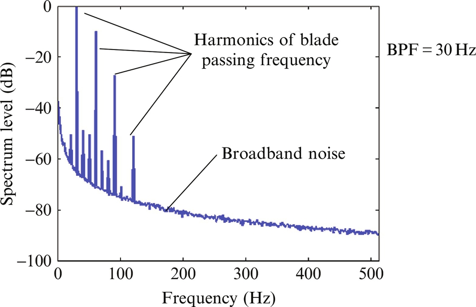
The best way to determine the relative importance of tone and broadband noise is to consider the narrow-band frequency spectrum of the signal. The Spectrum Level is defined as the root mean square of the signal, which has passed through a frequency filter of bandwidth Δf and centered on the frequency f. In rotor noise applications we always deal with harmonic signals, and it is important to use the Spectrum Level defined in this way rather than the Power Spectrum of the signal, which gives the signal energy per unit Hz. Fig. 16.2 shows a typical example of a rotor noise spectrum with a 3 Hz bandwidth for a three-bladed rotor at 600 rpm. The peaks define the tone noise and occur at the blade-passing frequencies, which in this case are multiples of 30 Hz. At higher frequencies the broadband random noise dominates the spectrum. This type of analysis is vital to the evaluation of rotor noise because it enables us to unambiguously distinguish between the tone and broadband noise, hence allows us to determine the most important noise source mechanisms.1
The primary sources of tone noise depend on the rotor tip speed, and the flow conditions in which the rotor is operating. Our understanding of rotor noise is based on the Ffowcs-Williams and Hawkings equation given by Eq. (5.2.13):

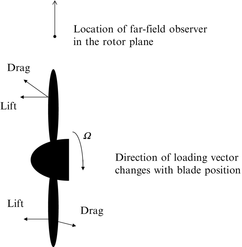
At low speeds the loading noise, given by the second term in Eq. (5.2.13), is usually the dominant source of sound. This indicates that the steady and unsteady pressure on the blade surface is the basis for the radiated sound. There are many effects that can influence the blade loading. If the propeller is operating with a completely clean inflow (uniform flow with no turbulence), which is rarely the case, then the blade loading is steady in blade-based coordinates, but the component of the force in the direction of the observer varies as the blade rotates. For example, consider the sound radiated out to the sides of the propeller in the plane of the rotor, Fig. 16.3. A far-field observer close to that plane “sees” a blade drag force that continuously changes direction, and so its component in the direction of the observer varies with time and a sound wave is generated. The same is true, but to a lesser extent, for the thrust force. The amount of load variation that is “seen” by the observer is obviously very dependent on the observer location, and the sound field is therefore very directional.
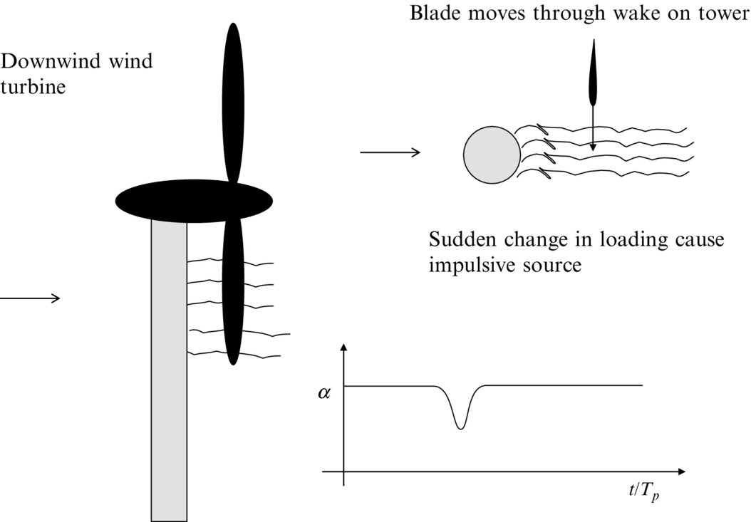
The sound caused by the time variation of the steady loading applies to all propellers, but it is a relatively weak source of sound compared to the unsteady loading. Most propellers operate in a nonuniform distorted inflow, and so their angle of attack varies continuously as they rotate as shown in Fig. 16.4. (For helicopter rotors this is a necessary design feature for level flight.) Smoothly varying changes of angle of attack are usually not very important, but when the blade encounters a sudden velocity deficit in the flow then the angle of attack change causes a rapid change in blade loading. The discussion of Eq. (5.2.13) showed that in the acoustic far field we can approximate ![]() , which shows that it is the time variation of the loading that generates sound. Consequently, a blade encountering a velocity deficit that causes a rapid change in loading can be a very efficient source of sound. A classic example of this is a wind turbine which can be designed so that the blades operate either upwind or downwind of the tower (Figs. 16.5 and 16.6). In the downwind design the tower causes a significant velocity deficit that the blade moves though, and so a strong acoustic pulse is generated (Fig. 16.5). In contrast if the wind turbine is designed so that the tower is downstream of the blades then the blades never pass through the velocity deficit, and they only encounter a small velocity perturbation as they pass the tower (Fig. 16.6). The upwind design of wind turbine is therefore significantly quieter than the downwind design. This principle applies to any propeller and, wherever possible, mounting of the rotor so that inflow distortions are minimized and slowly varying will reduce noise.
, which shows that it is the time variation of the loading that generates sound. Consequently, a blade encountering a velocity deficit that causes a rapid change in loading can be a very efficient source of sound. A classic example of this is a wind turbine which can be designed so that the blades operate either upwind or downwind of the tower (Figs. 16.5 and 16.6). In the downwind design the tower causes a significant velocity deficit that the blade moves though, and so a strong acoustic pulse is generated (Fig. 16.5). In contrast if the wind turbine is designed so that the tower is downstream of the blades then the blades never pass through the velocity deficit, and they only encounter a small velocity perturbation as they pass the tower (Fig. 16.6). The upwind design of wind turbine is therefore significantly quieter than the downwind design. This principle applies to any propeller and, wherever possible, mounting of the rotor so that inflow distortions are minimized and slowly varying will reduce noise.


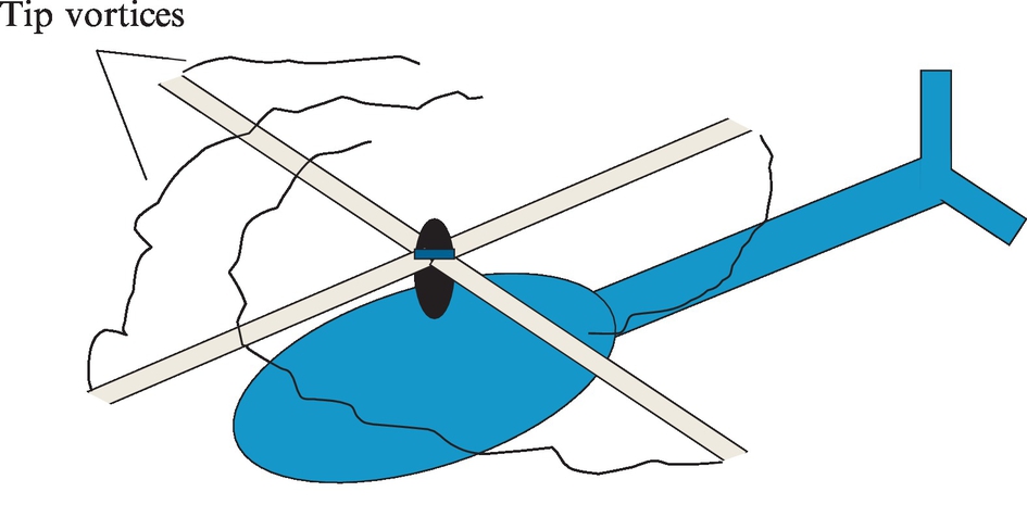
A special case of unsteady loading noise is caused by blade vortex interactions (BVIs) in helicopter rotors (Fig. 16.7). During forward flight the tip vortices of a helicopter can be ingested into the rotor and, given the right conditions, the helicopter blades can pass near the core of the vortex, and this causes a local, very rapid, change in angle of attack and a sudden change in blade load. This interaction emits a loud “thumping” sound and is often the dominant cause for complaints about helicopter noise. If the operational conditions are changed so that the wake is ingested in a different way then this noise source is eliminated, but unfortunately this is not always possible for some maneuvers.
In addition to unsteady loading noise the third term of Eq. (5.2.13) shows that there is a contribution from the blade surface motion that is referred to as thickness noise. We will show later that this is only important at tip speeds with Mach numbers in excess of 0.7. However, for high-speed helicopters and transonic propellers this source can be important. The mechanism for this source is the time varying displacement of fluid by the blade volume as it rotates. To the fixed observer in the acoustic far field it is as if the blade volume changes as it rotates, and this apparent variation in volume causes a sound wave in the far field. The simplest way to reduce thickness noise is to reduce the blade volume near the blade tip. If the blade thickness is halved in the tip region then the thickness noise is reduced by 6 dB, which is not insignificant and can be an effective way to reduce the noise from high-speed rotors.
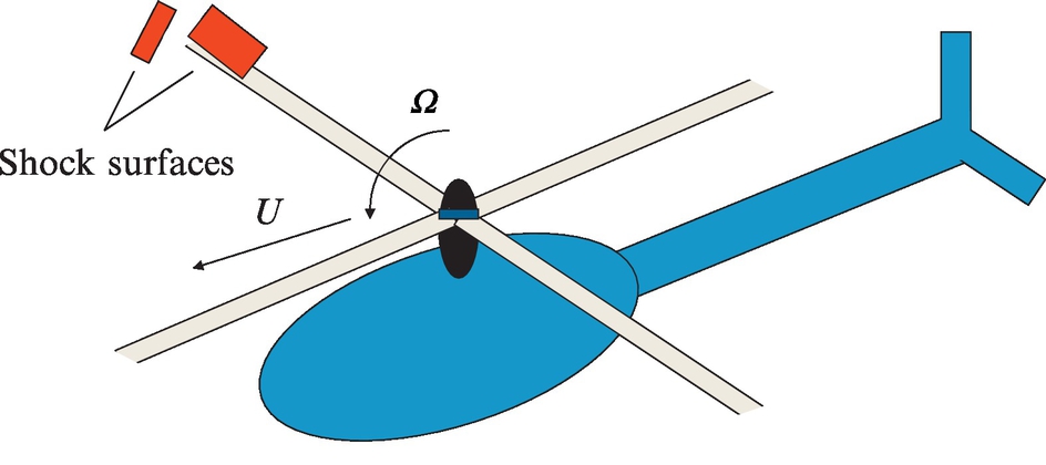
When the blade tip speed is transonic or supersonic then shock discontinuities can occur both on the blade surface and in the fluid surrounding the blade tips (Fig. 16.8). This is considered quadrupole noise because it is a source in the fluid volume as distinct from on the blade surface. From the observer's perspective, the shocks apparently change as the blade rotates, and so they generate sound. This mechanism can be just as important as thickness noise in some rotor designs. In general, the shocks are weaker if the blades are thinner, and so thinning of the blade tips is always advantageous for the reduction of transonic and supersonic rotor noise.
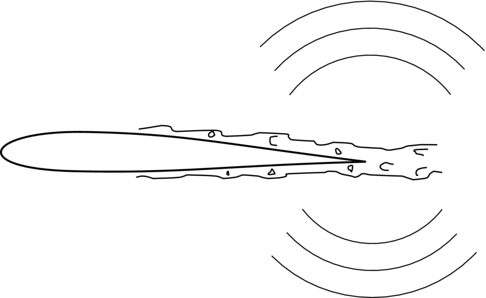
Broadband rotor noise is always caused by random variations in blade loading resulting from the interaction of the blades with turbulence. The turbulence is often generated upstream of the propeller and ingested into the rotor, but it can also be self-generated in the blade boundary layer or at the blade tips. An example where inflow turbulence is important is on ships where the propellers operate in a very disturbed flow underneath the hull. On helicopters, the trailing tip vortices that cause BVI noise can be surrounded by high levels of turbulence that generate broadband noise. This is referred to as blade wake interaction noise. The turbulence in the blade boundary layer does not generate much sound by itself, but when it passes the blade trailing edge the local boundary conditions change rapidly, and significant sound generation can occur (Fig. 16.9). As discussed in Chapter 15, this is trailing edge noise and is often considered as the most important mechanism of broadband noise generation in fans and propellers. Broadband noise from the turbulence at blade tips is not well understood at this time but may be important on low aspect ratio blades and should not be discounted as a possible noise source mechanism.
In the above we have summarized all the important source mechanisms for propeller and rotor noise. It is clear from this discussion that there are a number of competing mechanisms that are all important. In any particular application or set of operational conditions there may be several equally significant mechanisms or one may completely dominate. To determine the correct approach to sound reduction it is very important to be able to predict the noise levels from each of the sources described above. In the following sections we will discuss the prediction methodology for propeller and rotor noise and then, in Chapter 18, we will extend these ideas to ducted fans that have many of the same problems.
16.2 Time domain prediction methods for tone noise
16.2.1 Loading noise
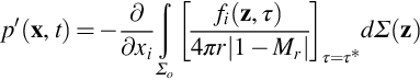
Loading noise is caused by the time variation of the compressive stress tensor pij on a blade surface as it rotates and may be predicted by the second term in the Ffowcs-Williams and Hawkings equation (5.2.13), which gives the radiated acoustic pressure as
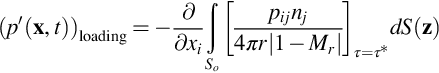
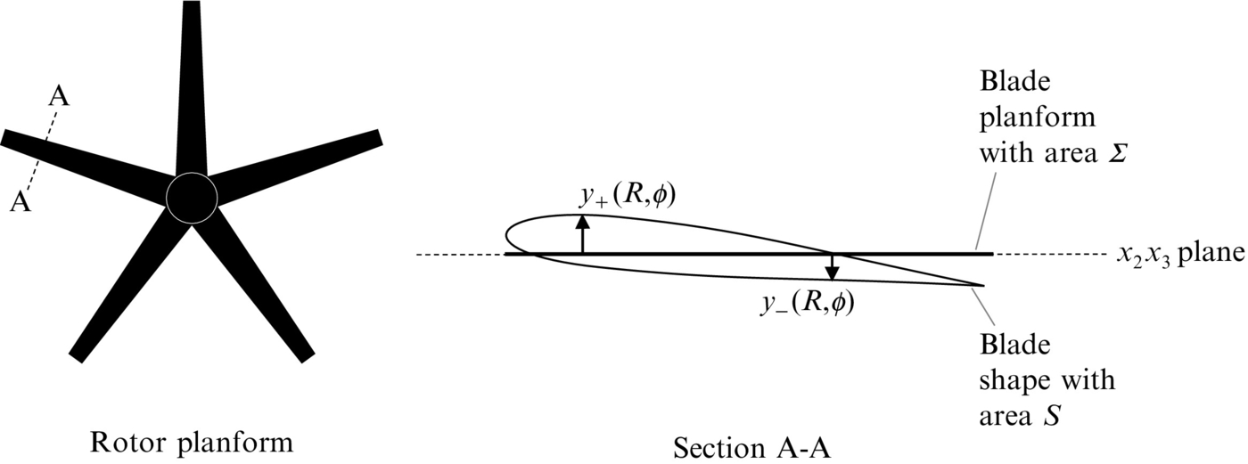
The surface integral in Eq. (16.2.1) should be carried out over the complete surface of the rotor blade, but in many instances it can be simplified to an integral over the blade planform. The planform is the projection of the rotor geometry into the rotor disc plane, as shown in Fig. 16.10. This approximation is valid if the blades are thin and the acoustic wavelength at the maximum frequency of interest is much larger than the blade thickness. We can then ignore the displacement of the upper surface from the lower surface and define the force per unit area applied to the fluid by the difference between the values of pijnj evaluated on the upper and lower surfaces for a given point on the blade planform (see Fig. 16.10). We define
where dΣ is the planform area in the disc plane (see Fig. 16.10) of the surface element dS. Substituting into Eq. (16.2.1) we obtain the thin airfoil approximation

For blades with lean and sweep there may also be a considerable displacement of the mean camber line of the blade from the rotor disc plane. This displacement should be included in the retarded time calculation that takes place inside the integral in Eq. (16.2.2).
If the variation of the surface loading fi repeats itself during each blade rotation, then tone noise results. To calculate the acoustic field, we need to know the precise variation of fi over the complete blade surface, as a function of emission time τ. However, there are some inherent difficulties with this requirement because the surface integral must be evaluated at a fixed observer time, and so the emission time τ will vary over the surface of the blade.
To address these difficulties, we use the approach pioneered by Farassat [1] and shift the spatial derivatives to source time, as explained in Section 5.2. The result was given by Eq. (5.5.2) for a far-field observer. If we project the blade loading onto the surface planform as described above, we obtain
To evaluate Eq. (16.2.3) we need to calculate the location of each surface element defined in the integrand at a given observer time.
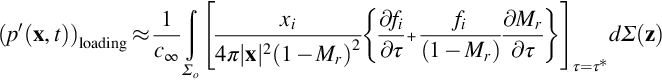
To proceed we need to define the coordinate system of the blade and the observer. There are several different choices for the coordinates, and care must be used in specifying the convention that will be used. In aircraft and marine propeller applications the convention [2] is to define coordinates (x,y,z) with x pointing in the direction of thrust. In helicopter applications the z coordinate is chosen in the direction of thrust. In actuator disc theory the x coordinate is chosen in the direction of flow through the propeller. In this chapter we choose the aircraft propeller convention with x or x1 in the direction of thrust as shown in Fig. 16.11. Furthermore, we need to choose the direction of blade rotation. A propeller rotating anticlockwise when viewed from upstream is defined as having “right-hand rotation.” If it rotates in a clockwise direction it is said to have “left-hand rotation.” We will choose right-hand rotation as shown in Fig. 16.11.
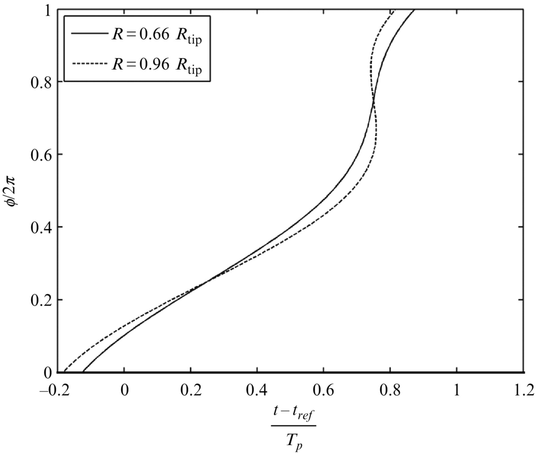
To evaluate the integrand in Eq. (16.2.3) we solve the equation t−τ−r(τ)/c∞=0, so we can specify the azimuthal location ϕ=ϕ1+Ωτ of each surface element as a function of observer time t, radius R, and azimuthal location ϕ1 in blade-based coordinates. For example, consider a rotor which is in the y2y3 plane at τ=0 and is moving with linear velocity (Uo,0,0) as shown in Fig. 16.11. In blade-based coordinates the location of each surface element is z=(0,R cos ϕ1, R sin ϕ1), and in fixed coordinates the surface element is located at y=(Uoτ, R cos(ϕ1+Ωτ), R sin(ϕ1+Ωτ)). The retarded time equation is given by t−τ−|x−y(τ)|/c∞=0, and to solve this equation we use an interpolation method. First we evaluate t using a uniformly spaced set of points τm=mΔτ in source time and then interpolate the results to obtain values of τ at fixed intervals in observer time tj=jΔt. Fig. 16.12 shows a plot of source location vs observer time for a stationary propeller rotating with a tip Mach number of 0.8 for source located at 30%, 60%, and 90% of the tip radius Rtip and an observer in the acoustic far field at x=(40Rtip, 30Rtip, 0). Notice how the curves cross at different observer times because the source at the outer radius is sometimes closer, and sometimes further from the observer as the blade rotates.
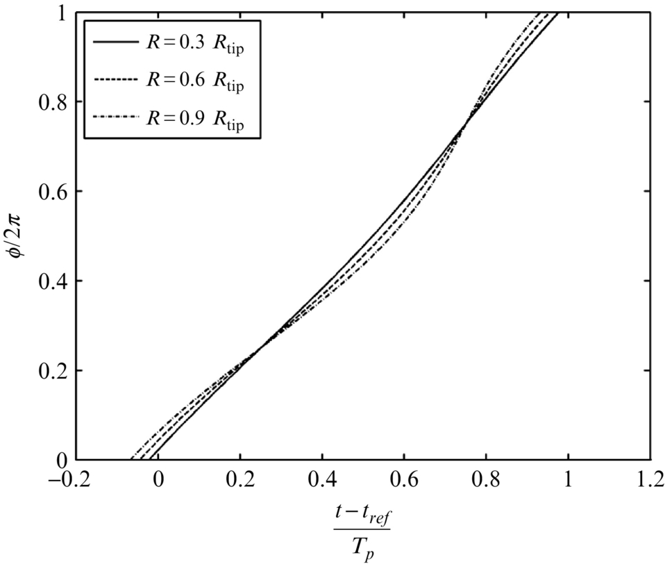
For blades with a subsonic tip speeds it is a relatively simple task to use this curve to compute the location of each blade element for uniformly spaced steps in observer time. However, for supersonic propellers this process becomes more difficult because the curve is no longer monotonically increasing, and we will return to this issue in Section 16.2.3.
The noise from steady loading is readily computed by defining the blade thrust FL and the blade drag FD for blade element of span ΔR located at R. (Note the sign convention requires that fi is the force per unit area applied to the fluid and is equal and opposite to the force per unit area applied to the blade.) For steady loading f1dΣ=−FL is constant, but the direction of the drag force varies with blade location, so f2dΣ=FDsin(ϕ1+Ωτ) and f3dΣ=−FDcos(ϕ1+Ωτ). Typically the drag force is about 10% of the thrust. The acoustic far field for each surface element can be computed using Eq. (16.2.3).
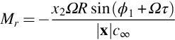
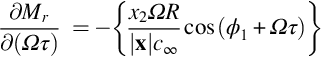
To illustrate a typical calculation, consider an observer at x=(40Rtip, 30Rtip, 0) for surface elements at 30%, 60%, and 90% of the blade radius. To evaluate Eq. (16.2.3) we need to define both the blade loading and the relative Mach number Mr, which is given, for x3=0 and Uo=0, by
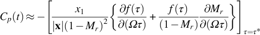
We then obtain a nondimensional acoustic signal defined as

with
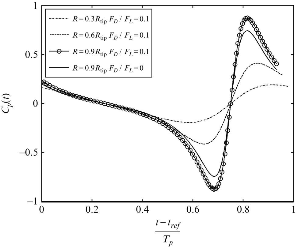
There are several important features to this result. First notice how the loading closest to the tip generates the most significant part of the signature because the rate of change of Mr is largest at this radius. Second note that if drag to lift ratio is small then the lift force dominates the calculation. In this case FD/FL=0.1 and the peak of the pressure pulse is only marginally increased by including the drag term (Fig. 16.13).
The magnitude of the signature in this example is small because the thrust force is constant during the rotation of the blade. However, if it has a harmonic time dependence, so f1dΣ=−FLf(τ), where f(τ)=cos(mΩτ), then Eq. (16.2.5) becomes
For large values of m the rate of change of f(τ) is much greater than the rate of change of the relative Mach number Mr, and so the radiated levels increase dramatically as shown in Fig. 16.14 for the case when m=10.
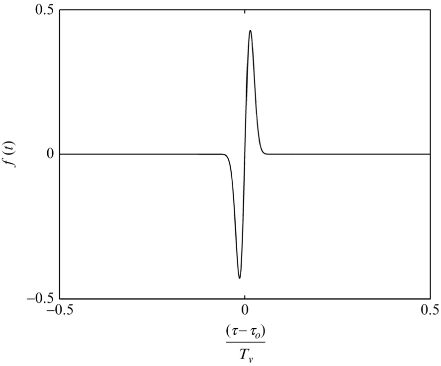
The peak signal level in Fig. 16.14 is approximately 30 times larger than in Fig. 16.13, showing the importance of the unsteady loading in these calculations. Also note how the frequency of the signature varies during the blade rotation. During the first part of the cycle the blade is moving away from the observer, and the frequency is lower than the source frequency because of a Doppler frequency shift. In the second part of the cycle the blade is moving toward the observer, and the Doppler shift increases the observed frequency so that it is higher than the source frequency. This effect is dependent on the observer position and is more dramatic in the plane of the rotor than along the rotor axis. The importance of unsteady loading is even more significant when the blade encounters a sudden change in angle of attack caused by an inflow distortion, an encounter with a wake, or a vortex in a BVI. To illustrate this, consider a fluctuation in thrust on the blade segment of span ΔR, located at R, given by
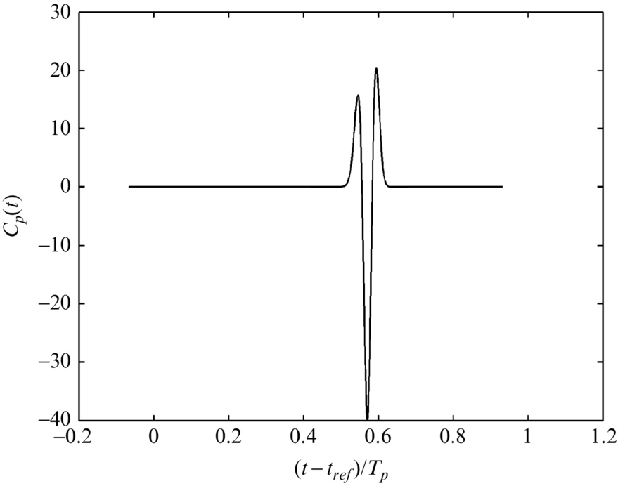
as illustrated in Fig. 16.15. The choice of Tv=0.02Tp gives a pulse which lasts for approximately one-tenth of the period of rotation in source time. The observed signature from this pulse at the observer location is given in Fig. 16.16 and is much shorter than the source signature as shown in Fig. 16.15. The source is at 90% of the blade span, and so the Doppler frequency shift can be large, and the observed signature becomes very impulsive, with a peak level that is much greater than for a harmonic variation in loading as shown in Fig. 16.14.
In the examples given above the signature from individual blade elements has been shown. To obtain a complete prediction of rotor noise the surface integral must be evaluated, and this can be achieved by numerical integration or summing the calculations for each blade element across the span at the correct retarded time. This is a relatively straightforward extension of the procedures described above providing that the blade surface loading is known as both a function of blade radius and azimuth. In low-frequency applications it is often reasonable to ignore the distribution of loading in the chordwise direction and replace fi with the sectional blade lift and drag per unit span for each blade radius. This assumes that the blade chord is small compared to the acoustic wavelength and is not always a good assumption, but it simplifies the calculations considerably and is a valid approach to obtain first estimates of blade noise signatures at low frequencies.
16.2.2 Thickness noise
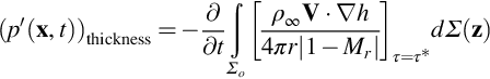
Thickness noise is described by the third term in the Ffowcs-Williams and Hawkings equation (5.2.13) which gives the acoustic field as

The evaluation of this source term for a propeller can be achieved using the method that was described in Section 16.2.1. The same procedure for evaluating the retarded time solution can be employed with the same limitations on numerical accuracy. The main difference is the appropriate evaluation of the source strength on the blade surface, which is easier in this case because it is defined exactly by the blade geometry.
As before we can replace the surface integral for thin blades by an integral over the blade planform in the rotor disk plane. We denote the upper and lower surface coordinates, displaced axially (in the y1 direction from the rotor disk plane) as y+(R,ϕ) and y−(R,ϕ). As shown in Fig. 16.10 we define the blade volume in terms of the upper surface function f+(R,ϕ)=y1−y+(R,ϕ)=0 and the lower surface function f−(R,ϕ)=y−(R,ϕ)−y1=0. The blade thickness is then defined by h=y+−y−. The normal to the blade surface is then given by n=∇f+/|∇f+| on the upper surface and n=∇f−/|∇f−| on the lower surface. It follows that on the upper surface
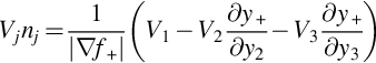
Similarly, on the lower surface

Since dS=dΣ/|n1|, ![]() , and |n1|=1/|∇f+| or 1/|∇f−|, we find that the contributions from the upper and lower surfaces can be combined to give
, and |n1|=1/|∇f+| or 1/|∇f−|, we find that the contributions from the upper and lower surfaces can be combined to give

Thickness noise can then be defined as an integral over the blade planform as
This shows how the blade thickness contributes to the source strength, and the result is independent of the blade angle of attack or camber. Consequently, this source is defined as “thickness” noise.
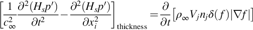
Evaluation of the source term in this equation at the correct retarded time can be challenging numerically, but an elegant alternative [1] simplifies this considerably. To derive this alternate form, we return to the Ffowcs-Williams and Hawkings equation (5.2.4) and only retain the thickness noise terms on the right-hand side. For an impermeable surface for which Vjnj=vjnj we obtain
However, for a body that does not deform as it moves we have, using Eqs. (5.1.12), (5.1.3),
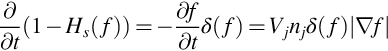
so the wave equation for thickness noise sources can be given in an alternate form as

The term (1−Hs(f)) represents the volume inside the moving surface, and so thickness noise can be considered as being completely equivalent to the sound from a displaced mass of fluid moving through a stationary medium, and this is referred to as Isom's result [1]. The solution to Eq. (16.2.15) is obtained following the procedures given in Section 5.2, with the double derivative with respect to time requiring integration by parts twice, followed by the integration (5.2.12), giving

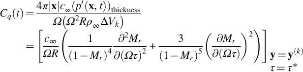
This result is relatively straightforward to evaluate numerically by breaking the volume of the blade down into acoustically compact volume elements of volume ΔVk, centered on y(k), and using ![]() , so
, so
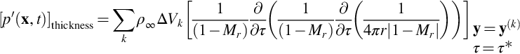
This result shows that thickness noise can be computed directly from volume elements within the blade, with the correct allowance for the propagation distance from the source to the observer. The signature from different parts of the blade planform will arrive at the observer at the same time, so the calculation is nontrivial, but it is tractable using numerical methods.
For an observer in the far field terms of order r−2 can be dropped, and this result simplifies to

We can normalize this result to obtain a nondimensional thickness noise pulse for each volume element as
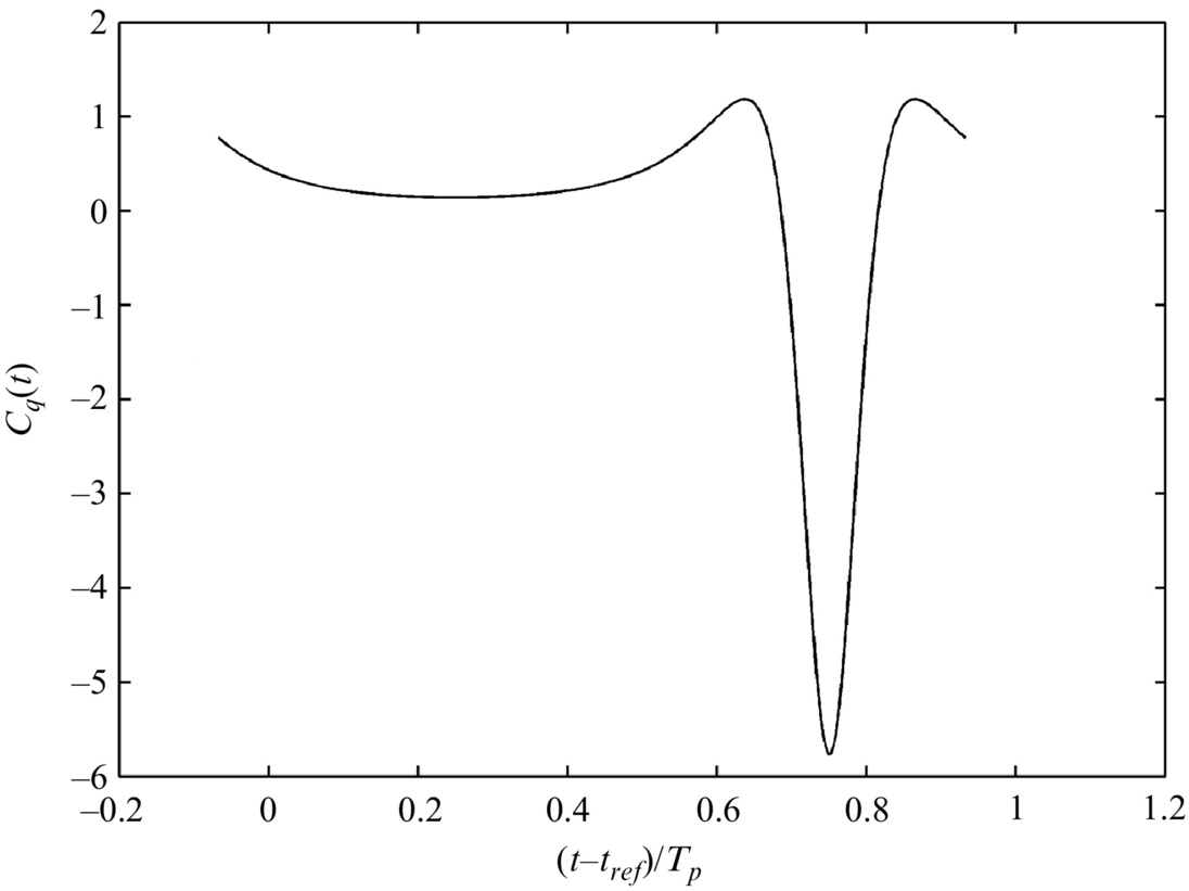
Using this normalization, we see that the thickness noise is scaled on an equivalent force equal to Ω2RρoΔVk, and so will depend on the blade volume. As an example the normalized signature for an observer at (40Rtip, 30Rtip, 0) and a source at 90% of the blade span, with tip Mach number Mtip=0.8, is shown in Fig. 16.17. The thickness noise gives a clearly defined pulse as the blade moves toward the observer, and its level exceeds that of a steady loading signature for high tip Mach numbers for the same equivalent blade loading. It is important to appreciate, however, that this calculation does not include all the effects of blade shape and retarded time across the blade chord, and more detailed calculations are required to define the exact thickness noise pulse.
16.2.3 Supersonic tip speeds
The calculations that have been described above are for blades with subsonic tip speed. When the blade tip Mach number exceeds one then a number of effects occur. These include the presence of shock surfaces in the flow and a singularity in the integrals (16.2.1), (16.2.2), and (16.2.14) when Mr=1. Another important issue for supersonic rotors is that there is no longer a one-to-one relationship between the emission time and the observer time. Fig. 16.18 shows the calculation of blade position for a given observer time for a supersonic rotor when the observer is in the plane of the rotor. Close to the blade tip it is seen that there are in fact three solutions for ϕ for an observer time of t/Tp=0.75. Consequently, the source strength from many parts of the rotor disc is concentrated at this instant of observer time, and a large impulsive peak in the sound signature is expected. Numerical calculations in and around this instant are clearly complex, and the reader is referred to the papers by Farassat [1] on the details of how to address this problem. Providing the correct asymptotic numerical coding is used, the time domain methods described above can be extended to supersonic rotors. However, as will be shown in the next section, many of these numerical difficulties with time domain methods are overcome if frequency domain methods are employed, at the expense, unfortunately, of other numerical issues.
16.3 Frequency domain prediction methods for tone noise
In this section we discuss the prediction of tone noise from a propeller or rotor using frequency domain methods [2]. These complement the time domain methods described in the previous section and also provide greater insight into the important physics of rotor noise.
16.3.1 Harmonic analysis of loading and thickness noise
In Section 16.2 we showed that the loading and thickness noise from a rotor could be defined as an integral over the blade planform, which was given by the combination of Eqs. (16.2.2), (16.2.14) as

For tone noise the resulting acoustic signature will be periodic, and the contribution from each blade will be repeated after each revolution. In this section we make use of this characteristic to evaluate the integrals in Eq. (16.3.1). We limit consideration to stationary propellers, but note that the theory can be readily extended to propellers and rotors in flight.
The signature from each blade is identical, and so if p1(x,t) is the signature from one blade in isolation, the signature from a rotor with B blades is
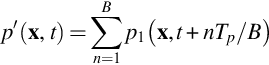
where Tp is the period of one rotation. Because the acoustic signature is periodic we can expand the signature from a single blade as a Fourier series of the type

where Ω=2π/Tp is the rotational frequency. Combining Eqs. (16.3.2), (16.3.3) then gives
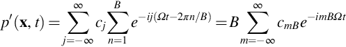
where we have made use of the fact that the sum over n is only nonzero when j=mB. The important feature of this result is that we can define the time history from a rotor with B blades from the Fourier coefficients of the time history from a single blade, but only the coefficients of order mB will contribute.
To determine the Fourier coefficients required in Eq. (16.3.3) we evaluate the integral
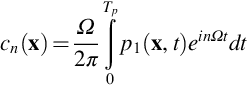
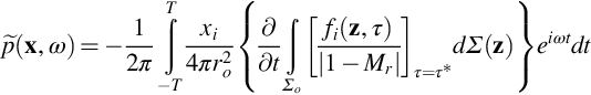
Combining this with Eq. (16.3.1) then gives
In the far field the differentiation of the first integral can be changed to a differential over time (see Section 5.2) using ![]() , where ro=|x| so that by using the properties of Fourier series we obtain
, where ro=|x| so that by using the properties of Fourier series we obtain

The integral over observer time can be changed to an integral over emission time because t=τ+r(τ)/co, and so the time differentials are related by dt=|1−Mr|dτ. It follows that since the source terms are also periodic with the same time scale, Eq. (16.3.7) reduces to

One of the most significant aspects of this transformation is that it eliminates the singularity that occurs when Mr=1, so the integrals are harmonic and well behaved for all blade speeds.
For an observer in the acoustic far field the integral over time in Eq. (16.3.8) can be evaluated directly. Consider the blade element at radius R and azimuthal location ϕ1 in blade-fixed coordinates, which is at y=(0, Rcos(ϕ1+Ωτ), Rsin(ϕ1+Ωτ)). Using the approximation r~ro−x·y/|x| the propagation distance from this element to the far-field observer is given by (see Fig. 16.11).
It is advantageous to specify the observer location in spherical coordinates so that
then
The final step in the analysis is to make use of the Fourier series expansion
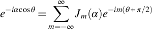
where Jm(α) is a Bessel function of the first kind of order m. This function has well-known properties and is readily available on most computational systems, so making use of it to simplify the analysis is advantageous. However, it is difficult to compute accurately for large orders, and so asymptotic formulae for the Bessel function are sometimes required. We can now write

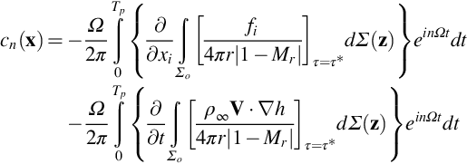
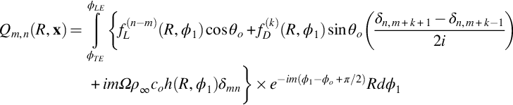
Combining all these results into Eq. (16.3.8) gives the Fourier series coefficients in a convenient form as

with the blade planform surface element defined as dΣ=Rdϕ1dR and the blade surface given by ϕTE(R)<ϕ1<ϕLE(R) and Ri<R<Rtip. The source term is given as
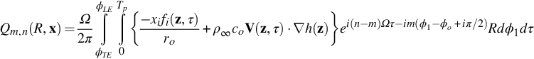
We have now reduced the problem to two relatively straightforward integrals. The first integral in Eq. (16.3.14) is over the blade span, and the second, in Eq. (16.3.15), gives the source term and requires integrals over the blade chord and the period of rotation. We will start by considering the case in which we can ignore the unsteady loading terms and limit consideration to only the steady loading and thickness noise terms. If the thrust per unit area on the blade surface is fL(R,ϕ1) and the drag is fD(R,ϕ1) then we have fi=(−fL,−fDsin(Ωτ+ϕ1), fDcos(Ωτ+ϕ1)), and we can define

Similarly, the thickness noise term may be simplified as in Section 16.2.2, as
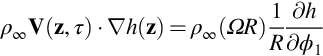
which is independent of time. Using these results in Eq. (16.3.15) then gives
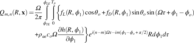
We have now completely specified the time dependence of the sources, and so the integral over time may be evaluated analytically. We note that both the thrust term and the thickness noise term are independent of time, and so their integral is only nonzero when n=m. Similarly, for the drag term the sine function may be split into the sum of two exponentials, and so the integral over time will only be nonzero when n=m±1. Finally, we note that the integral of the thickness noise term over ϕ1 can be carried out by parts, and providing h=0 at the leading and trailing edges we obtain
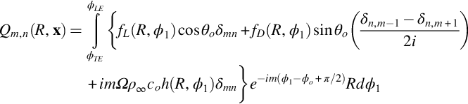
This provides a simple formula for the source term that can be readily evaluated. We still need to know the distribution of the thrust, drag, and thickness on the blade surface, but this can be obtained from the blade design characteristics. As a first approximation we can use a point-loading approximation, but this is inaccurate for the higher harmonics. One of the most important features of this result is that the integral over time has reduced the summation in Eq. (16.3.14) to only three values of m for a given harmonic n. The summation in Eq. (16.3.14) is therefore limited to only three terms (and can be further simplified by using properties of Bessel functions if required). This would not have been the case for unsteady loading because fL would then be a function of time. To show how unsteady loading can be incorporated into the calculation, we can assume that the loading is periodic in source time and can therefore be expanded as a Fourier series, so

and similarly for the drag term. Using this result in Eq. (16.3.18) and integrating over time shows that the integral will only be nonzero when n−m=k (or n−m=k±1 for the drag term), so we can rewrite Eq. (16.3.19) to include unsteady loading as
In this result the number of terms required in the summation over m in Eq. (16.3.14) has been significantly increased, and the expansion Eq. (16.3.20) may converge only slowly. So, the evaluation of Eq. (16.3.21) may be time-consuming, but the computational procedure is relatively straightforward. One of the advantages of this approach is that it allows the distribution of blade loading and thickness over the chord to be readily included in the calculation. It should also be noted that the radial integral in Eq. (16.3.14) includes a dependence on the Bessel function Jm(nΩRsinθo/co) which has a strong impact on the directionality of the acoustic field. These functions can be cumbersome to compute, but fortunately there are a number of asymptotic approximations, which simplify the task of computing the radial integral.
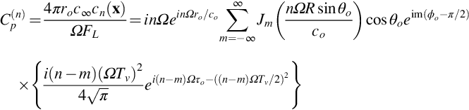
As an illustrative example we will calculate the Fourier series coefficients cn(x) for the Gaussian derivative impulsive blade loading given by Eq. (16.2.7). The loading coefficients in Eq. (16.3.20) can be calculated analytically in the limit that Tv≪Tp and are

where the terms in {} are required so that the force acts at a point. It follows then that

A contour plot of these coefficients is shown in Fig. 16.19 and clearly shows the importance of the terms with increasing m and n.

The nondimensional Fourier series coefficients of the acoustic signature are then obtained as
and the amplitude of these are plotted on a dB scale in Fig. 16.20. Note that the scale has a very large range, and the harmonics that contribute significantly are only those with indices <32. Evaluating the pulse observed in the far field from these harmonics reproduces the signature calculated directly using the time series approach, as shown in Fig. 16.16.
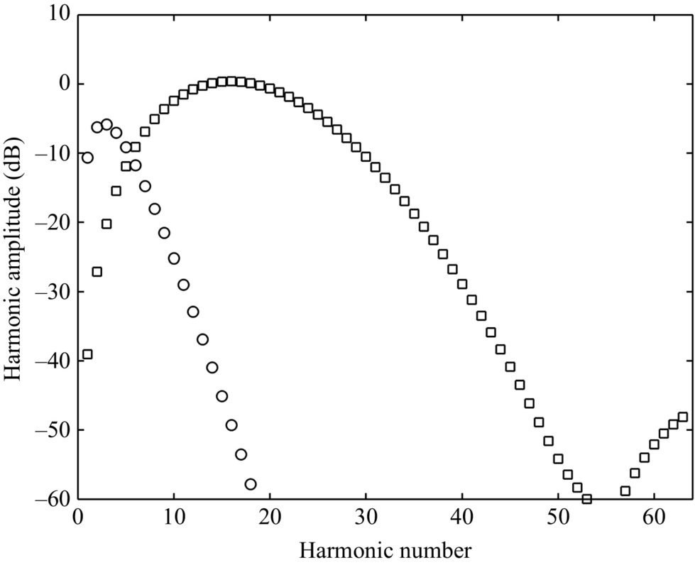
We can also evaluate the harmonics of the thickness noise pulse that was given in Fig. 16.17. The nondimensional form of these harmonics is given by

and these are also shown in Fig. 16.20. From this result we see that thickness noise tends to dominate for the lower harmonics, and unsteady loading noise dominates for the higher harmonics. Note also that for a rotor or propeller with B blades only the harmonics n=mB will contribute, so the contribution of thickness noise may be limited to the first two blade-passing frequencies.
16.4 Broadband noise from open rotors
In the previous sections we have discussed the harmonic content of the sound from a rotor, referred to as tone noise. This assumes that the acoustic sources are periodic, and the same signature is generated by each blade. In addition to tone noise, rotors also generate broadband noise that is not periodic with source fluctuations that are typically uncorrelated from blade to blade.
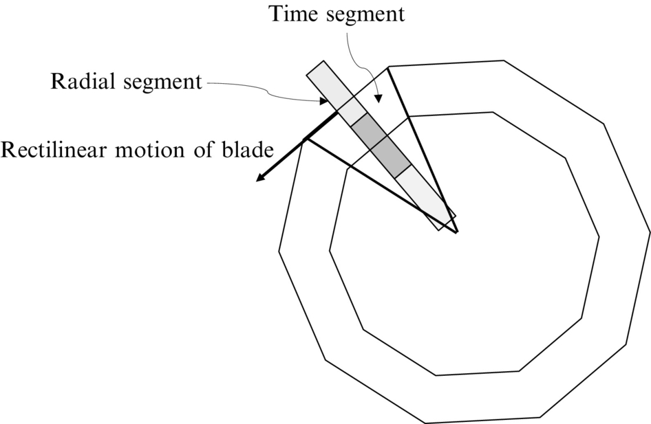
In Chapters 14 and 15 broadband noise sources on blades in a uniform flow were discussed assuming that the blade and observer were fixed and embedded in a uniform flow, as in a wind tunnel. To use these results for a blade that is moving relative to a fixed observer we can use Amiet's approximation, which applies when the time scale of the source fluctuations on a rotating blade is very much less than the time it takes for one rotor revolution. This will be the case for trailing edge noise sources that depend on the blade boundary layer, as described in Chapter 15, and for leading-edge noise sources when the lengthscale of the incoming turbulence is of the order of a blade chord or less. It also applies to a BVI and leading-edge noise when small-scale turbulence is stretched in the direction of the rotor inflow. In this limit Amiet [3] argued that the rotor noise signal could be accurately estimated by breaking down each revolution of the rotor into the suitable number of time segments and 10–15 radial segments as shown schematically in Fig. 16.21 and that (1) the blade could be assumed to be in rectilinear motion in each time segment and (2) the sources in each segment were uncorrelated, so the far-field sound was the incoherent sum of the mean square levels in each segment. The advantage of this approach is that the results from wind tunnel testing of fixed blades can be incorporated directly into the source terms for rotor noise, and this greatly simplifies the scaling of the results from model scale to full scale.
To apply Amiet's approximation the approach described in Section 16.3 will be used, but in this case we will evaluate the Fourier transform of the time history rather than its Fourier series coefficients. We start by evaluating the dipole source term in the Ffowcs-Williams and Hawkings equation for a single blade, which is
In general, we are interested in obtaining the spectrum of the far-field sound, and so we need to evaluate the Fourier transform of this equation with respect to time. As before we place the observer in the geometric far field and make the far-field approximation that ![]() , so the Fourier transform of Eq. (16.2.2) with respect to time is
, so the Fourier transform of Eq. (16.2.2) with respect to time is
where ro=|x|. The differential with respect to observer time is equivalent to multiplying the Fourier transform by −iω, and as in Chapters 14 and 15 we specify the unsteady loading per unit area on the blade in terms of the pressure jump in the direction of the blade normal (which will be different for each segment), so
and we obtain
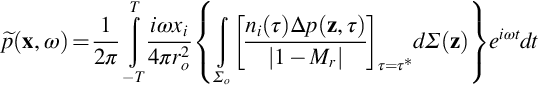
The integral over observer time can be shifted to an integral over source time by noting that as before dt=|1−Mr|dτ and t=τ+r(τ)/c∞, so we have
where T1 and T2 are the source times that correspond to the observer times ±T and tend to infinity.
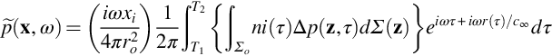
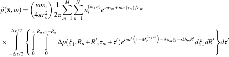
So far only the far-field approximation has been used, and so the result given by Eq. (16.4.3) can be used as a starting point for an exact analysis. However, if we make Amiet's approximation and segment the source time history into discrete intervals of length Δτ, the spanwise integral into finite parts Eq. (16.4.3) takes the form

where τm=mΔτ, τ1−Δτ/2=T1, and τM+Δτ/2=T2. Similarly, R1 is the inner radius of the blade, and RN+1 is the outer radius of the blade, and the segmentation in the radial direction does not have to be uniform. Also we have defined the distance from the blade leading edge in the chordwise direction as ξ1 and the spanwise direction as R.
In the geometric far field from the rotor we can approximate
where yi(τ) defines the location of the blade in fixed coordinates and can be evaluated from the blade location shown in Fig. 16.11 as

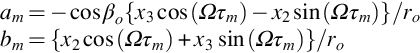
where the pitch angle βo is shown in Fig. 16.22. In Amiet's approximation both ΩΔτ and ϕ1 are limited to small angles, and so we can approximate
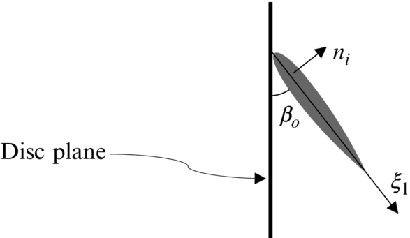

where Ur is the velocity of the blade in the direction of the observer.
Making the geometric far-field approximations the Fourier transform Eq. (16.4.4) then becomes
where k=ω/c∞, the displacement variables τ′=τ−τm and R′=R−Rn have been introduced, and the blade normal is assumed constant over the surface and defined for each segment, Fig. 16.21. Also we have defined the Mach number in the direction of the observer for each segment, and
Since the pressure jump is zero everywhere, but on the blade the integral over the chord in Eq. (16.4.6) can be extended to infinity in the ξ1 direction and becomes a wavenumber transform. However, the spanwise integral in each segment needs to be truncated at the edge of the segment, as discussed in Chapter 14, and some care is needed when applying this approach to sources that have significant spanwise correlation. By choosing the spanwise segments to be acoustically compact the phase variation can be eliminated, and the integral over the span is then well approximated by simply integrating the pressure jump over the span. Evaluating the integrals inside the curly braces then gives a result in terms of the wavenumber transform of the pressure jump, so
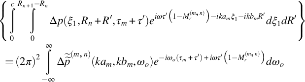
The integral over τ′ can then be carried out explicitly, and we obtain

This is the basis for Amiet's approximation and shows how the far-field sound can be directly related to the wavenumber transform of the surface pressure jump on the blades, evaluated at the wavenumbers corresponding to the waves in the acoustic far field. When k tends to zero this is the unsteady loading on the blade segment, and so scales as a dipole source as described in Chapter 4. However, at higher frequencies the results given in Chapters 14 and 15 must be used and can be inserted directly into this equation.
The size of the segment directly impacts the frequency scaling of the result. The integral over ωo represents a frequency filter that depends on the size of the segment used to separate the time steps in the process. The filtering process peaks when the source frequency is equal to the observer frequency reduced by a Doppler factor to account for source motion. The wavenumbers used in the evaluation of Δp are different from those used in Chapters 14 and 15 because in the present case the source is moving and the observer is stationary, whereas in the earlier examples the source and observer were stationary and the flow was moving. The consequence of this shift is that the source frequency is Doppler shifted to account for the source motion, but the spatial scales remain the same in both the observer-based coordinates and the moving source coordinates, so the wavenumbers are defined in the observer frame of reference.
The far-field spectral density from each segment can be defined by using the definition given in Eq. (8.4.13). If we assume that the segmentation is sufficient to resolve the frequency content of the signal so that the filter has no effect, we can specify the power spectral density from each segment as

and, if the fluctuations are statistically independent for each value of m and n, then the total far-field sound is obtained by summing the spectrum generated by each segment and multiplying by the number of blades. Amiet also pointed out that the averaging time in the fixed frame of reference would be different from the frame of reference of a moving blade by a factor of 1−Mr, and so Eq. (16.4.10) should also be corrected by this factor when using stationary blade data or models as inputs. This is expected to be a good approximation for trailing edge noise that depends on very small scale turbulence and is often suitable for leading-edge noise as well. Note that the expected value used in Eq. (16.4.10) is used in its most general sense in that the averaging is done on a blade-by-blade basis while it passes through each segment multiple times. This implies that the spectrum is obtained by averaging over many rotor revolutions and is a key part of this approach. It is important to appreciate that this result is equivalent to Eq. (14.3.1) and can be used with an inflow turbulence spectrum such as Eq. (14.3.4) to give the far-field sound from inflow turbulence. The overall characteristics of the far-field sound are then very similar to the noise from a blade that is not rotating, since the Doppler frequency shift in Eq (16.4.10) will tend to average out when the summation is applied across all the blade segments. The spectra shown in Fig. 14.6 are then expected to be typical of the spectra from a rotor when inflow turbulence dominates the far-field noise signature. For trailing edge noise, a similar conclusion can be drawn and modeling functions such as Eq. (15.2.10) can be readily adapted to provide the input required for Eq. (16.4.10). We will discuss how this is modified in situations where the segment signals are not statistically independent in the next section.
The valuable part of Eq. (16.4.10) is that it shows how measurements made in a wind tunnel on a stationary blade in a uniform flow can be applied directly to the sources on a rotating blade. The wavenumber spectrum of the blade surface pressure was defined for a blade in a uniform flow in Sections 14.3, and from Eq. (14.3.1) we have that

It follows that measurements made in the wind tunnel at the locations
and normalized as in Eq. (16.4.11) can be used a direct input into Eq. (16.4.10) for both leading-edge and trailing edge noise. This of course also applies to the Brooks, Pope, and Marcolini model for trailing edge noise (Section 15.3) and provides a suitable prediction method for fan noise.
16.5 Haystacking of broadband noise
In the previous section the broadband noise from a rotor was considered assuming that the flow scales that caused the sound were of sufficiently small that the pressure fluctuations on each blade segment, and each blade, were statistically independent and had the same statistics at all blade positions. This is a significant approximation, and we must also consider those situations where the blade pressure fluctuations are not uniform but vary at different points in the rotor plane, or are correlated from blade to blade. The first of these effects is referred to as amplitude modulation and is illustrated in Fig. 16.1C. The second is caused by the stretching of turbulent eddies as they enter the rotor and is sometimes referred to as inflow distortion noise.
16.5.1 Amplitude modulation
Amplitude modulation occurs when the source level on a rotating blade varies significantly with position. An example is a rotor operating in a very uneven inflow, such as the rotor operating near a wall that was discussed in Chapter 10. In this case the rotor blades pass through a turbulent boundary layer that extends over about one-fourth of the rotor disc plane. The noise levels from a particular blade are low when it is in the free stream flow outside the boundary layer, and all the leading-edge noise is generated when the blade passes through the high levels of turbulence in the boundary layer. The signal from each blade is therefore strongly modulated, but the modulation is partially mitigated by the number of blades in the rotor. If the blade count is low, then the effect of modulation is significant because there are times when no blade is in the region of high-level turbulence. However, if the blade count is high then there are always a number of blades in the region where noise is produced and the signal has very little variation with time. Another example is the effect of a nonuniform mean flow on trailing edge noise. If the nonuniform mean flow causes a significant change in blade angle of attack, then the trailing edge noise will be locally increased (or decreased as the case may be) and the far-field sound will have a signal that is modulated. In each case we will assume that the signal from each blade is uncorrelated, which will be the case for trailing edge noise but not always the case for leading-edge noise, and we will discuss the impact of blade-to-blade correlation in the next section.
To illustrate the effect that amplitude modulation has on the measured spectrum consider a source signal from each blade that can be modeled as fs(t), where s is the blade number and fs(t) is uncorrelated for different blades. If the signal is modulated as the blade rotates by a mean flow effect, then the modulation can be represented by the function g(t−sTp/B) for blade number s, where Tp is the time for one blade rotation and B is the blade count. The total signal is then

An example of the signal from one blade is shown in Fig. 16.23. This signal is only nonzero for one-fifth of the period of blade rotation, and the signals from successive blades should be added to this. Fig. 16.23B shows the signal for seven blades summed with the correct time delay. The signal appears to be continuous, and no periodic character is apparent from the overall signature, which is misleading.
The modulating function is periodic and so can be expressed as a Fourier series
and so the Fourier transform of the signal is given by

The power spectrum of the signal is given by

If we assume that the loading on each blade is statistically independent the double summation is reduced to a single summation, and if the base signal is statistically stationary and independent of blade number, then only those terms for which n=m will be nonzero, so

As an example we can consider a signal that is modulated by a periodic rectangular window of length Tg, where Tg=Tp/5 as shown in Fig. 16.23A, and assume that the source spectrum is given by

as shown in Fig. 16.23C. The signal has a time scale Ts=0.3Tp and the spectrum peaks at the frequency ω=Ω/2. When the signal is modulated and summed as in Eq. (16.5.1) the resulting spectrum is quite different and shows a series of peaks and an oscillatory level sometimes referred to as scalloping. The peaks do not occur at exact multiples of the rotation frequency or blade passage frequency because Sff peaks at a frequency that is nonzero. The spectrum, however, is quite different from that of a single blade as a direct result of the periodic modulation of the signal.
16.5.2 Blade-to-blade correlation
In Amiet's method it was assumed that the signals generated by each blade are statistically independent, and so there is no blade-to-blade correlation. This is a reasonable approximation for trailing edge noise that depends on the individual blade boundary layers and for situations where the length scale of the incoming turbulence is much smaller than the distance between the blades. However, it is known that when turbulence enters a rotor it can be stretched in the direction of the flow, and this extends its axial length scale. This stretching can be substantial and alone can result in a single turbulent structure being cut multiple times by successive blades so that the blade loading is correlated between the blades. This results in a quasiperiodic signal in the acoustic far field that includes bursts of pulses at the BPF and a sound spectrum with broadband peaks at near multiples of the BPF, referred to as haystacks. The criterion for this effect to occur is that the BPF should be significantly higher than the axial inflow speed Uo divided by the axial turbulence length scale BΩL/Uo ≫1. If this is a large parameter then blade-to-blade correlation needs to be considered, if not then Amiet's approximation can be applied.
This feature was originally identified by Sevik [4] for a propeller operating in grid-generated isotropic homogeneous turbulence. It was expected that the spectrum from this interaction would be a smooth function of frequency determined by the wavenumber content of the inflow turbulence. However, Sevik found that the spectrum included a series of humps that peaked at frequencies slightly above the BPF. It was later shown by Martinez [5] that the shifting of the humps from the BPF was caused by the pitch angle of the blades to the axial flow.
To illustrate the characteristics of blade-to-blade correlation, consider a series of pulses that persist for a limited period of time such as would be generated by a rotor with B blades cutting through an eddy at the blade-passing interval. The signature from each blade passage is the same, but the amplitude is modulated by the variation in the strength of the eddy as it passes though the rotor. A model for the time history of the sound produced by one eddy is

Here the envelope exp(−(Uot/L)2) defines the time variation in the strength of the eddy as it is convected through the rotor with axial velocity Uo. We model the observed signature of a single-blade passage through the eddy as f(t)=(Ut/Lo)exp(−(Ut/Lo)2) which is the same shape as the signal shown in Fig. 16.15. In this model L represents the axial lengthscale of the turbulence, Lo is the transverse lengthscale, and U is the flow speed relative to the blade.
Fig. 16.24A shows the time history modeled by Eq. (16.5.2). The spectrum of these pulses is shown in Fig. 16.24B for BΩL/Uo=Bπ/4 and BΩLo/U=2. The time scale of the interaction is relatively small in this case indicating that the axial flow speed Uo is large and the axial lengthscale L is small, so the blades only chop the eddy once, and the spectrum of the pressure time history is comparatively smooth. However, when the axial flow speed is reduced, and the lengthscale L is increased, the criterion for haystacking BΩL/Uo is increased. Fig. 16.25A gives the time history for the case when BΩL/Uo=Bπ. Because several blades interact with a single eddy the time history has multiple pulses at the blade-passing interval and the spectrum (Fig. 16.25B) shows clearly defined peaks at the blade-passing frequencies. This is the haystacking phenomenon.

Details of a time domain approach to this problem can be found in Glegg et al. [6].
16.6 Blade vortex interactions
When a helicopter undertakes a maneuver the trailing tip vortices shown in Fig. 16.7 can be ingested into the rotor and a BVI can occur. In certain flight regimes these interactions can occur when the axis of the vortex is parallel to the blade leading edge as shown in Fig. 16.26 for an advancing rotor.
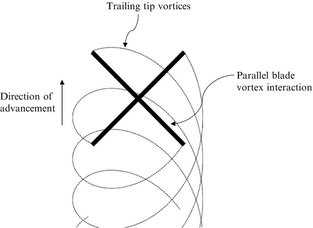
In Section 14.4 we showed that BVI depended on the angle that the axis of the vortex makes with the blade leading edge and the distance of the vortex core from the blade. Parallel BVIs are therefore the most important sources of sound. The characteristic sound of a BVI is a loud thumping sound that is caused by the impulsive unsteady loading described in both Sections 14.4 and 7.5 and, because the time scale of the pulse is usually short compared to the blade passage interval, the pulses are heard as individual events and can be analyzed as such. The spectrum from multiple pulses will then be given by the spectral harmonics of a single pulse at the blade-passing frequencies.
To calculate the acoustic field from a BVI we can use Amiet's method and consider the pulse to be short enough that the blade is in linear motion during the BVI. The BVI takes place at a specific point in the rotor disc plane, and so only one or two segments of the plane, as shown in Fig. 16.21, need to be included in the analysis. We can therefore use Eq. (16.4.9) to predict the far-field sound by only considering the specific values of m,n that define the location of the BVI. The pulses are of short duration, and so the segment time interval required in Amiet's method can be taken as being long compared to the pulse so that the integral in Eq. (16.4.9) is dominated by the sinc function and Eq. (16.4.9) is well approximated by

for the segment where the BVI occurs. To evaluate this expression, we require the wavenumber spectrum of the pressure jump across the blade, and this is obtained from Eq. (14.2.2) and takes the form
where the upwash velocity spectrum is given by Eq. (14.4.2) as

with ![]() .
.
The key features of this result are the angle of the BVI ϕv and the vortex miss distance h. As discussed in Section 14.4 if the interaction angle does not meet the criterion that
then no significant sound will be radiated because the vortex interaction with the blade leading edge moves subsonically (see Section 14.4). However, if this criterion is met then a BVI that radiates sound will occur and will depend on the miss distance of the vortex from the blade. This introduces a factor exp(−k13h) in Eq. (16.6.3) which is well approximated by exp(−|ωh/U|) and suppresses the high-frequency content of the gust when the miss distance h is large. It is seen from these results that both increasing the vortex miss distance h and the interaction angle ϕv reduce the sound level, and for noise control purposes they can be optimized to be an effective noise reduction tool.