The cascade blade response function
This appendix describes the solution to the problem defined in Section 18.3. The solution for the jump in potential across a blade that is part of a rectilinear cascade, as shown in Fig. 18.5, in response to a harmonic gust defined as woexp(−iωt+ik1x+ik2y+ik3z) is given by
Δϕˆ(x)=∫∞−∞D(α,k1,σ)e−iαxdα
where it is shown in Chapter 18, Ref. [12] that
D(α,k1,σ)=−iwo(2π)2(α+k1)J+(α)J−(−k1)−{∑n(An+Cn)ei(α−δn)ci(ω+αU)(α−δn)[J−(δn)J−(α)]}−{∑mBm(α−ɛm)[J+(ɛm)J+(α)]}
where
Ao=wo(ω−k1U)(2π)2j(−k1)δo=−k1
An=wo(ω+δnU)(2π)2(δn+k1)J′+(δn)J−(−k1)δn=κM+θn−1n>0
with
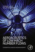
J′+(δn)=j′(δn)J−(δn)j′(δn)=(κM−δn)hβ24π(1−cos(δnd+σ)cos((n−1)π)){21n=1n>1
and the coefficients Bm are obtained as the solutions to the equations
{Bm}=[[1]−[Fmn][Lmn]]−1{[Fmn]{An}+AoGm}
where
Fmn=−ei(ɛm−δn)ci(ω+ɛmU)(ɛm−δn)[J−(δn)J′−(ɛm)]
Gm=−ei(ɛm−δo)ci(ω+ɛmU)(ɛm−δo)[J−(δo)J′−(ɛm)]
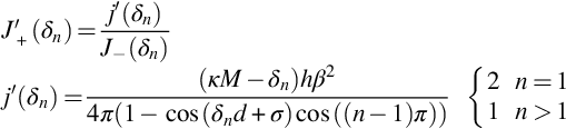
Lmn=i(ω+δmU)(ɛn−δm)[J+(ɛn)J′+(δm)]
The coefficients Cn are obtained from
Co=0Cn=∑mi(ω+δnU)(ɛm−δn)[J+(ɛm)J′+(δn)]Bmn>0
The split functions are defined as
J+(α)=κeβsin(κehβ)4π(cos(κehβ)−cos(ρ))∏m=0∞(1−(α−koM)/θm)∏m=−∞∞(1−(α−koM)/η−m)eΦ
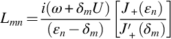
J−(α)=∏m=0∞(1−(α−koM)/ϑm)∏m=−∞∞(1−(α−koM)/η+m)e−Φ
The function Φ must be chosen so that both J+ and J− have algebraic growth as α tends to infinity and is given by
Φ=−i(α−koM)π{hβlog(2cosχe)+χed}
The singularities of these functions are given by
θm=−κ2e−(mπβh)2−−−−−−−−−−√ϑm=κ2e−(mπβh)2−−−−−−−−−−√
η±m=−fmsinχe±cosχeκ2e−f2m−−−−−−−√fm=σ+koMd−2πmd2+(hβ)2√
where tan χɛ=d/hβ. Finally, we have used the variables
M=Ue/coβ2=1−M2ko=ω/coβ2κ2e=k2o−(k3/β)2ρ=σ+koMd
so
j(α)=ζ4π{sin(ζh)cos(ζh)−cos((α−koM)d+ρ)}ζ=βκ2e−(α−koM)2−−−−−−−−−−−−−−√