
The theory of edge scattering
Abstract
The noise radiated from rotor or fan blades, or a stationary airfoil encountering turbulence, is primarily caused by the interaction of unsteady flow with the leading edge of the blade. In addition, blade boundary layer turbulence can only radiate sound if it encounters a surface discontinuity such as a trailing edge. Both these problems require the detailed analysis of the unsteady flow close to an edge. In this chapter we lay out the details of how edge scattering is calculated so that, in subsequent chapters, we can evaluate leading edge and trailing edge noise.
Keywords
Schwartzschild solution; Weiner Hopf method; Trailing edge response; Leading edge response
As we discussed in Chapters 6 and 7 the noise radiated from rotor or fan blades, or a stationary airfoil encountering turbulence, is primarily caused by the interaction of unsteady flow with the leading edge of the blade. In addition, blade boundary layer turbulence can only radiate sound if it encounters a surface discontinuity such as a trailing edge. Both these problems require the detailed analysis of the unsteady flow close to an edge. In this chapter we lay out the details of how edge scattering is calculated so that, in subsequent chapters, we can evaluate leading edge and trailing edge noise.
13.1 The importance of edge scattering
We have shown in earlier chapters that sound caused by a turbulent flow in the presence of an airfoil or fan blade is determined by the unsteady pressure on the blade surface. In general, we can model the blade, to first order, by a flat plate of finite chord as shown in Fig. 6.7. The far-field sound was shown in Sections 4.7 and 6.5 to be directly related to the wavenumber transform of the jump in surface pressure across the blade evaluated at the acoustic wavenumber. The physical interpretation of this result is that only waves that propagate across the surface at the speed of sound will couple with the acoustic far field. In principle this is also correct for blades that are acoustically compact in flows of very low Mach number, but in that limit the acoustic wavenumbers are close zero, and the wavenumber spectrum is equal to the net unsteady blade loading for all acoustic wavenumbers of interest.
On a smooth surface, pressure fluctuations associated with turbulence are convected at a speed that is less than (or equal to) the local flow speed, and in most cases of interest this is subsonic. The far-field sound can therefore only be caused by the interaction of the turbulence with an edge, or a discontinuity on the surface, both of which scatter wave energy into acoustic waves. The two most important examples are leading edge noise, where turbulent gust impinges on the leading edge of a blade, and trailing edge noise in which turbulent boundary layer pressure fluctuations are convected downstream across the blade trailing edge. In this chapter both these problems will be considered.
Amiet [1,2] addressed the problems of leading and trailing edge noise by using the solution to the Schwartzschild problem, which was developed for electromagnetic wave scattering in the presence of a semi-infinite half plane. We will derive the solution to this problem using the Weiner Hopf method, which is of general applicability and will be extended to cascades of blades in Chapter 18. The solution to the Schwartzschild problem for electromagnetic waves only applies to a stationary surface in the absence of flow, and so we will also describe how these results can be extended to sound radiation in a uniform flow.
13.2 The Schwartzschild problem and its solution based on the Weiner Hopf method
13.2.1 The boundary value problem
The scattering of hydrodynamic pressure waves by a trailing edge can be modeled by considering a surface pressure disturbance traveling downstream over a semi-infinite plate, as shown in Fig. 13.1. The disturbance is expressed in terms of Δp, the pressure difference between the top and bottom sides of the plate.
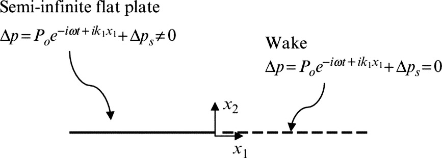
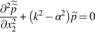
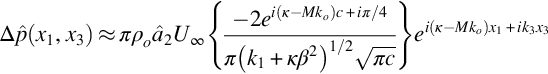
We assume that the pressure jump Δp in the absence of the trailing edge (located at x1=0) is given by Poexp(−iωt+ik1x1) and that the flow Mach number is so small that the mean flow can be ignored in the first instance. Note that we will allow for the possibility that the wavenumber k1 may have a small imaginary part allowing for decay or growth of the disturbance with x1. Both at and downstream of the trailing edge there can be no pressure jump across the surface (the Kutta condition), and so an acoustic wave field must be added that exactly cancels the incident pressure disturbance for x1>0, x2=0. The scattered acoustic field p must satisfy the acoustic wave equation, and also the boundary condition that ∂p/∂x2=0 on the surface of the plate to match the non-penetration boundary condition. If we initially limit consideration to two dimensions with no mean flow, then the scattered acoustic field is given by the solution of the Schwartzschild problem. This defines a scattered acoustic field with a harmonic pressure fluctuation ![]() that satisfies the wave equation and the boundary conditions:
that satisfies the wave equation and the boundary conditions:
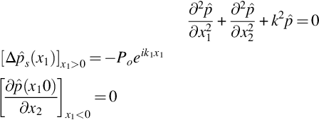
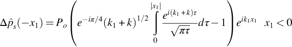
Schwartzschild showed that this problem can be solved to give the pressure jump over the plate caused by the scattered wave as
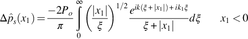
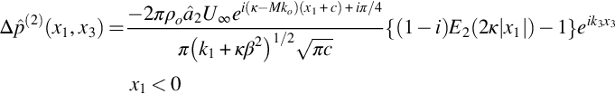
which on evaluation of the integral gives
where E2(x) is a modified Fresnel integral defined as

which is a function that appears often in the theory of edge scattering in several different forms.
13.2.2 Obtaining the Schwartzschild solution using the Weiner Hopf method
The result given by Eq. (13.2.2) is specific to the boundary value problem given by Eq. (13.2.1). However, we can obtain the same result in a way that may be extended to more general cases by considering the scattering in more detail. This will lead to formulations for leading edge noise and far-field radiation that do not follow directly from Eq. (13.2.2).
To obtain Eq. (13.2.2) we start by taking the wavenumber transform of the wave equation with respect to x1, defined such that
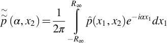
(Note: since this is a wavenumber transform we have chosen the exponential to have a negative sign.) The wave equation then reduces to
and the solution to this equation is
where
The branch cut for γ is chosen so that Re(γ)>0. The presence of the plate implies that the wave field can be discontinuous across the plate where x2=0, and so we can define separate solutions for the regions x2>0 and x2<0. The additional boundary condition that we have is that the acoustic waves must decay at large distances from the plate, and we can only meet that condition if we set B(α)=0 when x2>0 and A(α)=0 when x2<0. While the plate can support a pressure jump, the normal derivative of the pressure on x2=0 must be continuous for both x1>0 (where there is no plate) and x1<0 (where it is zero). The pressure gradient is therefore

and so A(α)=−B(α), and the acoustic field caused by the scattered waves is given by the inverse of Eq. (13.2.4) (i.e., the inverse wavenumber transform)
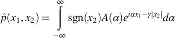
and allows for a pressure jump across the plate.
In order to solve the unknown function A(α) we use the wavenumber transform of Eq. (13.2.6) on the surface x2=0+ given by

However, the boundary condition is different for x1>0 and x1<0, so we write this as
where

and
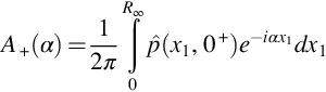
The integrand of Eq. (13.2.9) is known from the boundary conditions of the problem, but A−(α) remains as an unknown. To make use of the non-penetration boundary condition we define the chordwise Fourier transform of the pressure gradient normal to the plate, given by

where the lower limit of the integral is zero because the pressure gradient is zero when x1<0. However, by differentiating Eq. (13.2.6) we see that the pressure gradient is given by the inverse Fourier transform
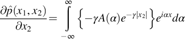
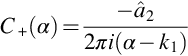
and thus C+(α) is given by the terms in curly brackets at x2=0+, which using Eq. (13.2.7) is
This completely defines the boundary value problem with the conditions set by Eq. (13.2.1). The functions A+(α) and A−(α) are required to define the acoustic field using Eq. (13.2.6), but unfortunately only A+(α) is known, and both A−(α) and C+(α) are unknowns, and so it appears that this problem is underdetermined and cannot be solved with these boundary conditions alone.
13.2.3 The radiation condition and the Weiner Hopf separation
In solving the wave equation, we used the radiation condition that requires the sound field to decay at large distances from the surface. The same condition applies far upstream or downstream from the edge, and we can use this additional boundary condition to solve for the two unknowns in Eq. (13.2.11). To ensure that waves decay as |x1| tends to infinity we require that the surface pressure has the asymptotic values

where C, D, and β are real positive constants. (There is no need to impose a restriction on the pressure gradient for negative x1 since the gradient is zero here anyway.) The same condition should also be required for the incident pressure disturbance, and this is achieved by requiring that Im(k1)>β. This apparently implies that the incident wave decays from a large value upstream, but this issue can be addressed by assuming that the incident wave is of finite extent in the upstream direction, as would be the case in a real flow.
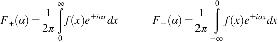
To show how this additional boundary condition can be used, we make use of some well-known properties of the Laplace transform, which is defined by the transform pairs
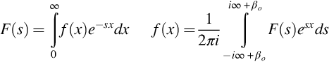
This transform is relevant to the problem being considered because it is essentially the same as the Fourier transform defined in Eq. (13.2.9) over the positive values of x1, so, for example,
Laplace transforms are used extensively in control theory and are often applied to determine if a system is stable or unstable. By definition they represent a function that is zero for x<0, and the system is stable if it does not have exponential growth as x tends to infinity. The criterion to prevent growth at infinity is that the Laplace transform of the function should have no poles, branch cuts, or other singularities on the right side of the complex s plane where Re(s)>0, as shown in Fig. 13.2.
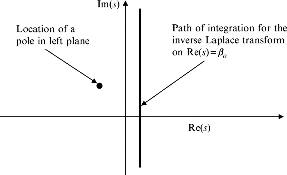
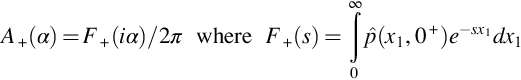
If the function f(x) decays exponentially for large x>0, so f(x)<Cexp(−βx), where C and β are positive real constants, then the Laplace transform converges when Re(s)>−β, and all the singularities of F(s) lie to the left side of the path of integration shown in Fig. 13.2. Since we wish to impose the boundary condition that the scattered field decays for large |x1|, the criterion can be restated as requiring that all the singularities of F+(s) lie in the region of the s plane where Re(s)<−β. We can then impose this restriction on the boundary condition given by Eq. (13.2.12) to eliminate one of the two unknown functions and obtain a complete solution.
However, before we proceed we must define the Laplace transforms of the other terms in Eq. (13.2.11). Since the pressure gradient normal to the plate is zero when x1<0 we can define its Laplace transform as in Eq. (13.2.12), by the function G+(s), and so C+(α)=G+(iα)/2π. However, for the pressure upstream of the edge, the Laplace transform must be defined by reversing the direction of integration, so (using ξ=−x1)
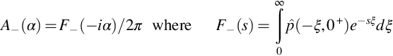
So, the boundary condition may be written as
The functions in this equation are analytic in different parts of the s plane as shown in Fig. 13.3.

It follows that the right side of Eq. (13.2.14) only converges in the strip −β<Re(s) <β. This is important when we evaluate the inverse Laplace transform defined as

which is only valid if F(s) converges along the path of integration. The inversion of Eq. (13.2.14) is therefore required to be carried out by choosing −β<βo<β and is only possible if β>0.
We also need to be very specific about the definition of the function γ. This is a multivalued function and, to meet the radiation condition, is required to have a positive real part. To ensure that this is the case on the path of integration Re(s)=βo we choose the branch cuts that are shown in Fig. 13.4, and using the criteria given in Appendix B, define


and require that k has a small positive imaginary part that moves the branch points away from the path of integration as shown.
All the terms in Eq. (13.2.14) are now defined along the path of integration required for the inverse Laplace transform. However, on the left side of this equation G+(s) represents a function that is zero upstream of the edge and decays at large x1, so it can have no singularities for Re(s)>−β. The same is therefore true for the right-hand side of this equation. This gives the additional restriction that is needed to solve Eq. (13.2.14) for the two unknowns, and we can manipulate the terms so that this criterion is met, which is the basis of the Weiner Hopf method. First divide by J+(s) so that
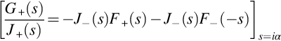
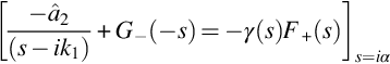
The first term on the right side of this equation is a mixture of functions that have nonanalytic features for both positive and negative values of real s. However, it can be split into two parts, one which exactly cancels the second term on the right (which only has singularities for Re(s)>β) and the second that has no singularities on the left side of the s plane. This separation is dependent on the form of F+(s) which is given by the boundary condition for x1>0 in Eq. (13.2.1) with the pressure at x2=0+ being taken as half of the pressure difference Δps, and thus
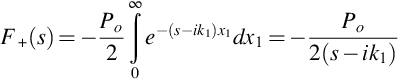
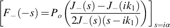
This has a simple pole at s=ik1 that is shown in Fig. 13.4. By removing the residue at the pole we can then write Eq. (13.2.15) as

If we take the inverse transform of this equation along the imaginary axis s=iα the right side will give a function that is zero for x1>0 because all the terms are analytic for Re(s)<0 as shown in Fig. 13.3. Similarly, the left side will give an equation that is zero for x1<0 (providing that J+(s) is not zero when Re(s)>0). The only possible solution therefore is that the two sides are independently equal to zero (or equal to a function whose inverse transform is zero). We then obtain the solution for the unknown function that gives the pressure on the upstream surface as
Using the definitions in Eq. (13.2.16) the pressure on the upstream part of the surface can be obtained from the inverse Laplace transform of
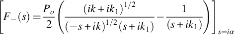
as a function of ξ=−x1. Both terms in this equation have a pole at s=−ik1 in the right half plane that individually would cause a growing wave, but since the residues of the terms cancel we can move the path of integration to the right of the pole and substitute s=s1+ik, so the inverse transform (designated by L−1{}) is

Standard tables give the inverse Laplace transform of the functions 1/(s+a) and 1/s1/2, which should be combined as a convolution integral when multiplied together. We then obtain the pressure jump across the surface as 2f(ξ) where
which is identical to the result given by Eq. (13.2.2).
13.2.4 Generalized Fourier transforms and Laplace transforms
The analysis given in the previous section was based on Laplace transforms to obtain the solution to the Schwartzschild problem. In much of the literature (Noble [3], Morse and Feshbach [4]) the Weiner Hopf method is carried out using Generalized Fourier transforms of the type
These are equivalent to the approach given above with ±iα replacing the Laplace transform variable s. The advantage of the current approach is that there are well-documented tables of Laplace transforms and their inverses that are readily available and can be used to simplify the results, and so this is the reason that this approach has been used here. Generalized Fourier transforms can always be obtained from Laplace transforms, providing the correct substitutions are made. However, care must be exercised in the location of branch cuts in the s plane as a function of different variables. If the wrong branch cut is chosen, then the incorrect result will be obtained.
The other benefit of the present approach is that, while different authors use different conventions for Fourier transforms, the convention for Laplace transforms is universal, and so there is little ambiguity in the final result.
13.3 The effect of uniform flow
In Chapter 6 we discussed thin airfoil theory and showed how the unsteady loading of an airfoil in a uniform flow could be modeled by a flat plate at zero angle of attack that satisfied the convective wave equation. In trailing edge noise applications, we need to account for the mean flow over the surface, and so the Schwartzschild problem described in the previous section must be modified to account for the flow. In addition, the pressure perturbation over the surface is usually three dimensional, and so the two-dimensional analysis used in Section 13.2 must be extended to the three-dimensional case.
To account for these effects, the perturbations in pressure and velocity potential must satisfy the convective wave equation (6.4.3) so that

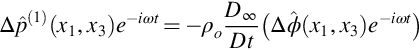
These equations account for the convection of the sound waves by the uniform free stream and are thus no different than the sound propagation equations for a stationary medium derived in Chapter 3, except that the time derivative is expressed in the frame of reference of an observer who is moving relative to the medium rather than one who is fixed with respect to it. The pressure perturbation on the surface can still be considered harmonic, but is convected downstream in the direction of the flow, and can include a harmonic spanwise variation so that the boundary condition given by Eq. (13.2.1) is modified to
where k1=ω/Uc with Uc being the convection speed of the incident pressure perturbation. Since the incident disturbance is harmonic in time and the surface geometry is independent of the spanwise direction, we can specify the scattered acoustic field as
so that the scattered pressure has the form ![]() . Substituting this form into the convective wave equation we obtain
. Substituting this form into the convective wave equation we obtain

with M=U/c∞, β=(1−M2)1/2, and k=ω/c∞.
To solve this equation, we proceed as in Section 13.2 and take its wavenumber Fourier transform with respect to x1, giving

We solve this equation as in Section 13.2 subject to the same boundary conditions for the pressure jump across the surface and the continuity of the pressure gradient and obtain the solution as before, so the three-dimensional pressure is given in the same form as Eq. (13.2.6) by

where in this case
The Schwartzschild problem can be solved in exactly the same way as was done in Section 13.2 the only difference being in the definition of γ, which can be taken into account by factorizing γ and specifying, for s=iα

The unsteady surface pressure in the no flow case was shown to be determined by the function J−(s)=(s+ik)1/2, and so the effect of flow is to modify the result by replacing k with κ+koM in the final result, so from Eq. (13.2.3) we obtain
This extends the two-dimensional analysis to the three-dimensional case with flow and gives a procedure for simplifying the rather complex problem of a convected flow to a tractable problem.
The blade response to an incident pressure disturbance is important in the evaluation of trailing edge noise, as will be discussed in detail in Chapter 15. In this case the nondimensional response gte(x1, k1, k3) is defined so that
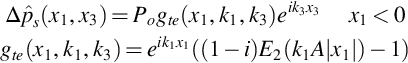
where A=1+(κ+koM)/k1. Some care needs to be used when evaluating κ because this can be imaginary for large values of k3. However, for surface pressure fluctuations that couple to the acoustic far field κ must always be real valued as will be discussed in Chapter 14. For the case when k3=0 we find that A=1+Uc/c∞(1−M) which is always greater than 1. The effect of the mean flow on the surface pressure only appears as the factor of (1−M) in the definition of A and tends to make the response more rapid in the vicinity of x1=0.
13.4 The leading edge scattering problem
The unsteady loading on a flat plate of finite chord caused by an unsteady upwash gust can also be evaluated in a compressible flow by using a modification to the Schwartzschild problem described in the previous sections. However, the effect of finite chord is important in this problem, and so we need to include the effect of both the leading edge and the trailing edge of the blade in the solution. This cannot be achieved in closed form, but an iterative method based on the successive approximations of the blade by semi-infinite flat plates converges quite quickly and is a good approximation to the complete response. The approach is to first solve the problem of an upwash gust incident on a semi-infinite flat plate and then add a correction based on the Schwartzschild solution described in Section 13.2 to ensure that there is no pressure jump across the wake downstream of the blade trailing edge. This correction however introduces a small jump in potential upstream of the leading edge, and so additional terms need to be added to correct this. However, as we will show below this is a relatively small correction that can usually be ignored.
13.4.1 The leading edge response
To solve the first-order problem of an upwash gust encountering a semi-infinite flat plate, as shown in Fig. 13.5, we will use the same approach as was used in Section 13.2 but with the velocity potential as the dependent variable in the wave equation rather than the pressure.

The wave equation in this case is defined by Eq. (13.3.1); the potential of the scattered acoustic field has the form ![]() , and the boundary conditions are
, and the boundary conditions are
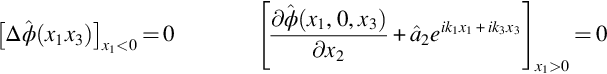
for a harmonic upwash gust convected by the mean flow, so k1=ω/U∞ in this case. The solution can be obtained as before by taking the wavenumber transform of the wave equation. The final result will be of the same form as Eq. (13.3.5) with the velocity potential replacing the unsteady pressure and the requirement that the gradient of the velocity potential is continuous across the plate. The boundary conditions can then be defined using the half-range transforms given by Eqs. (13.2.7) through (13.2.10), with the subscripts referring to the upstream or downstream part of the x1 axis, so
In this case A−(α)=0 and
As before this equation has two unknowns A+(α) and C−(α), so we need to use the radiation condition as |x1| tends to infinity to find a solution. The procedure used in Section 13.2 is followed again by writing the boundary condition in terms of the Laplace transforms defined in Eq. (13.2.14) with the velocity potential as the dependent variable and s=iα, so
We need to separate the terms in this equation that contribute to the wave field upstream or downstream of the leading edge, and this is achieved by factorizing γ(s), as in Eq. (13.3.6) identifying those terms that have singularities in the right or left side of the s plane. From Fig. 13.4 we see that the factored equation takes the form

As before the inverse Laplace transform of the left side of this equation gives a function that is zero for x1>0, while the right side gives a function that is zero for x1<0 providing that the imaginary part of k1 is greater than zero. We then obtain the Laplace transform of the jump in potential across the surface downstream of the leading edge as

or, in terms of the wavenumber spectrum of the potential jump,

The inverse Laplace transform of Eq. (13.4.2) gives the potential jump, but in this case it is useful to evaluate the unsteady pressure jump
and since (ω−αU∞)=(k1−α)U∞ and the pressure jump is the inverse transform of 2A(α), we obtain

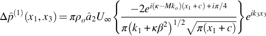
The inverse transform can be evaluated from tables, and we find that

(where we have used β2(k1+koM)=k1). The important conclusion from this result is that the pressure jump at the sharp edge has a square root singularity and tends to zero at large distances downstream of the leading edge. The implication is that both the pressure jump and the particle velocity at the leading edge are infinite, but in reality the velocity at the edge will be limited by viscous effects and the details of the geometry. The modeling that has been used here is based on thin airfoil theory, which ignores that rounding of the leading edge of a blade. When the details of the rounding are included in the analysis the leading edge pressure jump will be quite different as discussed in Chapter 7 for incompressible flow.
13.4.2 The trailing edge correction
For a blade with a finite chord these results need to be corrected for the effect of the trailing edge and the Kutta condition. We can calculate a correction that satisfies the trailing edge boundary condition by using the trailing edge scattering theory described in Section 13.2. However, this result is for a semi-infinite flat plate, and so there will be a residual error that occurs at the blade leading edge. Successive corrections can be calculated using the methods described here, but first we will consider the first-order trailing edge correction that is obtained by solving the trailing edge boundary value problem described with the incident pressure jump given by Eq. (13.4.5). Since the origin in the leading edge problem is at a distance c upstream of the trailing edge the result given by Eq. (13.4.5) must be redefined with the origin at the trailing edge, giving
Carrying out the full Weiner Hopf procedure on this function is difficult, but a simplified result is obtained in the high-frequency limit if the amplitude variation with x1 is ignored, and we approximate the pressure near the trailing edge as
We can then use the analysis given in Section 13.2 to find the trailing edge correction as the additional pressure jump
If the origin of the coordinate system is relocated back to the leading edge, we obtain the corrected nondimensional surface pressure function as

The corrected solution given by Eq. (13.4.6) is only an approximate solution, but includes the major effects caused by the trailing edge, and ensures that the Kutta condition is satisfied. The pressure jump includes a discontinuity upstream of the leading edge because we have used a trailing edge correction that assumes it is the same as the response of a semi-infinite flat plate upstream of the trailing edge. However, for large arguments we find that
so this correction is small when the blade chord is large compared to the acoustic wavelength.
In conclusion we have developed expressions for the response of a flat plate airfoil to a harmonic gust and obtained the unsteady surface pressure distribution, which can be used to calculate the unsteady loading and the far-field sound. These results are crucial to the calculation of sound radiation from thin airfoils and, although the derivation is complex, the results are important to our understanding of the problem. We will discuss the features and characteristics of the results in the following chapters.