Trailing edge and roughness noise
Abstract
Airfoils and other fluid dynamic devices generate noise as a result of turbulence and unsteadiness in the boundary layers and other viscous flow regions that grow from their surfaces. This is called self-noise. In this chapter we focus our discussion on self-noise generated by turbulent boundary layer over a sharp trailing edge and the flow of the boundary layer over a rough wall. The fundamental origins of these noise sources are discussed. We present both Amiet's prediction method for trailing edge noise and the empirical approach of Brooks, Pope, and Marcolini. The scattering theory of roughness noise is explained, and the possibility of using designed-rough surfaces to radiate specific portions of the boundary layer pressure fluctuations is demonstrated.
Keywords
Turbulent boundary layers; Trailing edge noise; Roughness noise
In the last chapter we examined leading edge noise—noise generated by an airfoil subjected to free stream unsteadiness. Airfoils and other fluid dynamic devices also generate noise as a result of turbulence and unsteadiness in the boundary layers and other viscous flow regions that grow from their surfaces. This is called self-noise. In this chapter we focus most of our discussion on self-noise generated by turbulent boundary layers, specifically the flow of a turbulent boundary layer over a sharp trailing edge and the flow of the boundary layer over a rough wall.
15.1 The origin and scaling of trailing edge noise
Trailing edge noise is fundamentally a consequence of the interaction between unsteadiness in the flow and the sharp corner formed by the trailing edge of a lifting surface. Consider this situation in its most idealized form, illustrated in Fig. 15.1. The trailing edge is modeled as a semi-infinite flat plate of zero thickness immersed in a uniform flow with a sweep angle Λo. This approximation, in which the leading edge is ignored, is realistic as long as the airfoil chord remains large compared to the acoustic wavelength of the sound produced.

Turbulence generated by the boundary layers formed on both sides of the plate is convected over the trailing edge. Sound generated in this scenario can be characterized in terms of a solution to Lighthill's equation. One strategy, first considered by Ffowcs Williams and Hall in 1970 [1], is to employ a tailored Green's function chosen to satisfy the rigid wall boundary condition on the plate. The sound produced is then given by Eq. (4.5.6) purely in terms of the Lighthill stress tensor,
where we have expressed the sound field in terms of the pressure fluctuations it produces. Ffowcs-Williams and Hall solved this equation using an exact expression for the Green's function and by ignoring the viscous and nonisentropic contributions to the Lighthill stress tensor, approximations consistent with high Reynolds number and low Mach number flow. In this case the sound source is only a function of the Reynolds stress fluctuations Tij=ρvivj. Simplifying the result for turbulence close to the edge and for a far-field observer, they developed an expression for the radiated sound

As illustrated in Fig. 15.1, θx and θy are the angles of the observer and source points, x and y, measured from the plate in a plane perpendicular to its edge; ry is the source distance from the edge, in that plane; and ϕx is the angle of the observer measured from the edge. The result is expressed in terms of the polar velocity components about the trailing edge vr and vθ and the acoustic wavenumber k.
Eq. (15.1.2) reveals immediately that there is no significant sound generated by velocity fluctuations parallel to the trailing edge. This is consistent with expectations of the theory of vortex sound (Section 7.1, discussed for trailing edge applications by Howe [2]) from which we would expect the streamwise component of the vorticity to have no impact on the sound generated.
In order to examine the scaling of the sound implied by Eq. (15.1.2) we note that since the mean velocity of the flow must be parallel to the flat plate, then, for example,
We can ignore the first term since it is steady and does not contribute to the sound, and the last term on the basis that it is negligible if the turbulent fluctuations are small compared to the mean velocity. If we restrict ourselves to low Mach number flows then we also ignore the density fluctuation contribution to the Lighthill stresses and replace ρ with ρo. Applying similar considerations to νθ2 and vrvθ, Eq. (15.1.2) becomes

where subscript i=1,2 for the cylindrical components vr and vθ, and f1 and f2 involve only trigonometric functions of θy. Note that the form of Eq. (15.1.2) is unchanged if we choose to use Cartesian velocity components inside the integral. We can now estimate the spectrum of the far-field sound as
where we have introduced the two-point velocity cross spectrum,
and also the constant u representing the velocity scale of the turbulent fluctuations. Now, the frequency of the sound will be controlled by the frequency with which eddies pass the trailing edge, U/L, and thus we expect k=U/Lc∞, where L is the lengthscale of the turbulence. We also expect L to be the scale of the distance between the sources and the trailing edge, ry and ry′. Incorporating these observations, Eq. (15.1.4) becomes

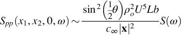
The inner integral in this expression is the volume under a weighted correlation coefficient function and is expected to scale with the cube of L. The outer integral will multiply this result by the span of the trailing edge b, and a distance proportional to L in each of the other two directions where the weighting in ry′ is effective. In conclusion, we have that the far-field sound spectrum will scale approximately as
where S(ω) provides the shape of the normalized pressure spectrum and has units of seconds.
This expression reveals a number of characteristics typical of trailing edge noise. Most importantly trailing edge noise is seen to scale approximately on the fifth power of the flow velocity, or more accurately, as the fourth power of the velocity times the Mach number. This clearly demonstrates that at low Mach number the presence of the trailing edge greatly amplifies the direct sound radiation from the turbulence which, in the absence of the trailing edge, would scale as U4M4 according to Eq. (4.4.11). Interestingly, trailing edge noise is also slightly more efficient than the classical dipole scaling given by Eq. (4.4.8), much like high-frequency leading edge noise. Trailing edge noise also has a cardioid directivity, cos2(½θx) (Fig. 15.2), in which the loudest sound is directed upstream and no sound propagates directly downstream. Sound is emitted above the airfoil in antiphase with that emitted below. Eq. (15.1.6) reveals that trailing edge noise can be reduced by sweeping the trailing edge, relative to the flow it experiences (though this effect may be partly compensated for if accompanied by a corresponding increase in the trailing edge length), or by decreasing the scale of the turbulence L. Note that Eq. (15.1.5) suggests that trailing edge noise can also be controlled if the turbulent sources can be moved away from the edge, increasing ry.

The most important results from Ffowcs-Williams and Hall's analysis are these scaling and directivity observations. More detailed analysis requires estimation of the complicated two-point velocity spectrum function that forms the source term.
15.2 Amiet's trailing edge noise theory
A different strategy for the analysis of trailing edge noise is to seek a solution through Curle's equation (4.3.12). In this case we will have a quadrupole contribution from the sound generated directly by the turbulence and a dipole contribution from the sound produced by the unsteady loading on the airfoil which, of course, is an integration of the pressure fluctuations experienced on the airfoil surface. Based on the scaling arguments outlined in Section 4.4, we expect the dipole contributions to dominate in low Mach number flows.
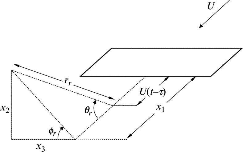
Amiet [3,4] exploited this observation to develop an analytical approach to the quantitative prediction of trailing edge noise. Like Ffowcs-Williams and Hall he used the thin-airfoil theory approximation of a flat plate (Fig. 15.3) in a uniform flow in the x1 direction. Statistically identical turbulent boundary layers are assumed to form on either side of the airfoil.

Amiet's theory takes advantage of the fact that the spectral form of the wall pressure fluctuations imposed by a turbulent boundary layer on a flat plate, in the absence of the trailing edge, is well known. At least in the idealized circumstances pictured in Fig. 15.3, the convected vorticity that defines the boundary-layer turbulence will not be modified as it flows over the trailing edge since no flow distortion occurs. The changes in the pressure field that occur in the vicinity of the trailing edge, including the radiation of sound, are therefore an irrotational response of the flow to the removal of the non-penetration condition and the imposition of the Kutta condition at the trailing edge. Amiet modeled this situation by treating the pressure fluctuation as having two components, one representing the undisturbed boundary layer and the other resulting from the response of the trailing edge to this disturbance.
We begin with Eq. (6.5.5) for the dipole sound radiated by a flat plate airfoil in terms of the pressure difference it experiences. Integrating this expression gives the sound expressed in terms of the wavenumber transform of the acoustic pressure

where the wavenumber arguments to Δp are given by Eq. (6.5.6)
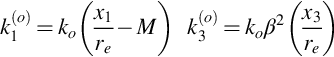
and thus account for the convection of the sound waves in the uniform stream surrounding the airfoil. Note that here ko=ω/(β2c∞), ![]() , and β2=1−M2. Using the definition of the wavenumber transform of the pressure, adapted from Eq. (4.7.12), the full wavenumber transform of the surface pressure jump is related to the spanwise wavenumber transform as
, and β2=1−M2. Using the definition of the wavenumber transform of the pressure, adapted from Eq. (4.7.12), the full wavenumber transform of the surface pressure jump is related to the spanwise wavenumber transform as

We can therefore rewrite Eq. (15.2.1) to give the far-field sound in terms of the pressure differences at a given chordwise location on the airfoil
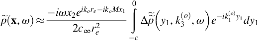
Note that in Eqs. (15.2.2), (15.2.3) we have prescribed the limit so as to recognize the finite size of the airfoil, which is taken as extending from −c to 0 in the chordwise direction y1. We are interested in the spectrum of the far-field sound, rather than the acoustic pressure at any particular instant, and this we can obtain using Eq. (8.4.14) as
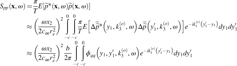
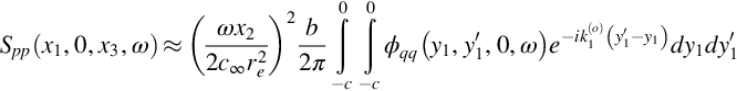
where ϕqq is the spanwise wavenumber transform of the cross spectrum of pressure difference fluctuations between any two points on the airfoil surface. Note that we have taken the range ±R∞ of the spanwise Fourier transform to be the airfoil span, of ±b/2, effectively assuming that this is very large compared to the spanwise scales of the turbulence encapsulated in ϕqq. We will restrict ourselves to an overhead observer for whom ![]() , and so
, and so
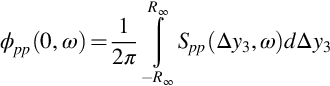
In order to specify ϕqq we prescribe the boundary-layer pressure fluctuations in two parts. The first part is the pressure fluctuations that would be produced by the boundary layer in the absence of the trailing edge pbl. In terms of the wavenumber frequency transform of pbl this is

Using Taylor's frozen flow hypothesis we assume that pressure fluctuations do not evolve and are convected downstream along the airfoil surface at a uniform speed Uc so that k1=K1≡ω/Uc. Following the discussion at the end of Chapter 8, we expect this to be 60–80% of the boundary-layer edge velocity. This means that the wavenumber transform of the boundary-layer pressure fluctuations can be written as
Thus Eq. (15.2.5) can be reduced to

Note that because of the overhead observer simplification we will only need to consider contributions to pbl at zero-spanwise wavenumber, k3=0. The second part of ϕqq is the pressure fluctuation that results from the response of the trailing edge to this disturbance, which is given by the Schwarzschild solution detailed in Chapter 13. For a pressure perturbation,
the Schwarzschild solution Eq. (13.3.9) gives the trailing edge pressure response as
So, for all wavenumber components, the total pressure fluctuation on the airfoil surface will be

Taking the Fourier transform in y3 and time, we obtain
For the response function gte we ignore the leading edge of the airfoil and use the result for the trailing edge response of a semi-infinite airfoil, from Eq. (13.3.9)
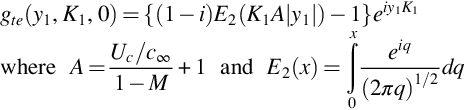
We expect this to be a good approximation as long as the airfoil chord remains large compared to the acoustic wavelength and thus K1c≫1. Substituting into Eq. (15.2.6) we obtain
Now, the spectrum of the pressure difference across the airfoil will be twice the spectrum of the pressure itself, as we do not expect the boundary-layer pressure fluctuations to correlate between the two sides. So,

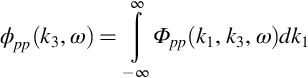
where ϕpp is the spanwise wavenumber frequency spectrum of the undisturbed boundary-layer pressure fluctuations. That is, in terms of the full wavenumber frequency spectrum Φpp,
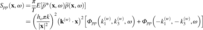
Substituting from Eq. (15.2.8) into Eq. (15.2.4), we recover
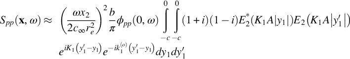
The integrals inside over y1 and y1′ can be separated and are conjugates of each other, and so our final result can be written as

or,
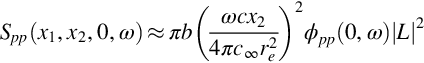
where ![]() , the integral inside the absolute value, is Amiet's [3,4] generalized lift function. Note that the sound predicted by Eq. (15.2.10) is twice that given by Amiet since we are accounting for both airfoil boundary layers. The integration defining
, the integral inside the absolute value, is Amiet's [3,4] generalized lift function. Note that the sound predicted by Eq. (15.2.10) is twice that given by Amiet since we are accounting for both airfoil boundary layers. The integration defining ![]() can be done analytically, but Amiet [4] argues that the integrand should be modified to soften the effects of the leading edge limit (at −c) which otherwise implies unsteady loading generated by the plane-wall boundary-layer pressure fluctuations pbl acting at the sharp leading edge of the flat plate. These do not exist for a real airfoil where the boundary layer originates at a rounded leading edge. To avoid this problem, the complex exponential in Eq. (15.2.6) is modified to include a term that ensures decay with distance from the trailing edge, i.e., the exponential becomes exp(K1y1[i+ɛ]) and the undisturbed boundary-layer contribution to
can be done analytically, but Amiet [4] argues that the integrand should be modified to soften the effects of the leading edge limit (at −c) which otherwise implies unsteady loading generated by the plane-wall boundary-layer pressure fluctuations pbl acting at the sharp leading edge of the flat plate. These do not exist for a real airfoil where the boundary layer originates at a rounded leading edge. To avoid this problem, the complex exponential in Eq. (15.2.6) is modified to include a term that ensures decay with distance from the trailing edge, i.e., the exponential becomes exp(K1y1[i+ɛ]) and the undisturbed boundary-layer contribution to ![]() is then assessed in the high-frequency limit as ɛ tends to zero. With this adjustment Amiet [4] gives the magnitude of
is then assessed in the high-frequency limit as ɛ tends to zero. With this adjustment Amiet [4] gives the magnitude of ![]() as
as
where

Note that the source term ϕpp in Eq. (15.2.10) is related by Fourier transform to the spanwise cross spectrum of surface pressure fluctuations
Thus we can write
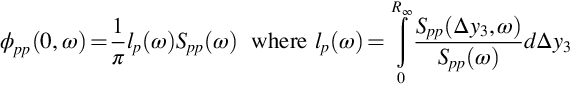
and express the source term as the product of a frequency-dependent spanwise pressure lengthscale lp(ω) and the autospectrum of the surface pressure fluctuations Spp(ω). At any given frequency we expect the scale of the turbulence in the streamwise and spanwise directions to be the comparable and therefore anticipate that lp(ω) will vary as U/ω.
To determine the scaling and directivity implied by Amiet's result we note, as before, that the frequency of the sound ω will be determined by the flow speed divided by the turbulence scale U/L. Roughly speaking we also expect the pressure spectrum to vary as ρo2U4S(ω). The scaling of |![]() |2 can be determined from the fact that
|2 can be determined from the fact that ![]() . Thus for large K1c (implying, not unreasonably, that the eddies are small compared to the chord length)
. Thus for large K1c (implying, not unreasonably, that the eddies are small compared to the chord length)

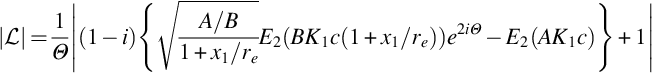
since at low Mach number A≈1 and B≈M. The realism of this characterization can be seen in Fig. 15.4 which shows that (K1c/2)2|![]() |2M is equal to 1 over a substantial range of frequencies and Mach numbers with an error of less than ±1 dB. Indeed estimating |
|2M is equal to 1 over a substantial range of frequencies and Mach numbers with an error of less than ±1 dB. Indeed estimating |![]() |2 as (K1c/2)−2M−1 may be sufficiently accurate for some applications. Finally, we note that ignoring convective effects, re=|x|, x2/re=x2/|x|=sinθ, and x1/re=cosθ, where θ is the directivity angle from the downstream direction defined in Fig. 15.3. Combining these observations, we conclude that in the absence of convective effects
|2 as (K1c/2)−2M−1 may be sufficiently accurate for some applications. Finally, we note that ignoring convective effects, re=|x|, x2/re=x2/|x|=sinθ, and x1/re=cosθ, where θ is the directivity angle from the downstream direction defined in Fig. 15.3. Combining these observations, we conclude that in the absence of convective effects
 |2M vs. Mach number and wavenumber, evaluated for Uc/U=0.8 and x1/re=0.5, in decibels.
in complete agreement with Ffowcs-Williams and Hall's result (Eq. 15.1.6). Note that accounting for convective effects [5] produces a more complex directivity in terms of the angle θr, the observer location measured from the retarded source position (Fig. 15.3), giving
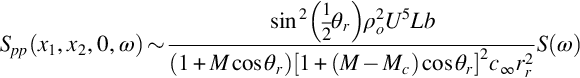
where rr is the distance from the retarded source position to the observer.
Amiet's major contribution is in formulating a method in which well-defined and established empirical information can be used to predict the form and level of a trailing edge noise spectrum from first principles. As an example, we consider sound predictions for a NACA 0012 airfoil at zero angle of attack. The data [6], shown in Fig. 15.5, reflect a chordlength of 0.23 m and a span of 1.22 m, with an observer 3 m directly overhead over the mid-span of the trailing edge. The flow speed is 55.5 m/s giving a chord Reynolds number close to 660,000. The airfoil boundary layer is heavily tripped, and the trailing edge displacement thickness δ* is estimated as 2.4 mm. From the discussion following Eq. (9.2.12) we take uτ/Ue=4%. We would expect, approximately, δ/δ*=8 and Uc/Ue=0.8 (see Section 9.2.2). With these parameters we can use Eqs. (9.2.29) or (9.2.37) to estimate the autospectrum of the boundary-layer pressure fluctuations Spp(ω). For lp(ω) we use Amiet's suggested relation

Note that we could alternatively get an expression for lp(ω), or for ϕpp(0,ω) as a whole, by integrating one of the wavenumber spectrum models for the wall pressure presented at the end of Chapter 9.
The comparison of predictions performed using the boundary-layer spectrum models and the data are presented in Fig. 15.5. The predictions have been scaled to one-third octave band SPL to make this comparison, by multiplying by the frequency and by (21/6−2−1/6). Overall the spectrum is predicted quite well, including some features of the shape. The predictions appear some 5 dB below the measurements at lower frequencies. This type of disagreement is not unexpected. The adverse pressure gradient experienced toward the rear of the airfoil would be expected to increase the energy of larger boundary-layer eddies, and the amplitude of the pressure fluctuations they produce, and increase the spanwise lengthscale over which the pressure fluctuations correlate lp when compared to a flat plate boundary layer. Using pressure spectra and scales measured on the airfoil itself has been shown to improve agreement between measurements and predictions [5,7].
15.3 The method of Brooks, Pope, and Marcolini [8]
While Amiet's theory establishes the fundamental relationship between trailing edge noise and the boundary-layer pressure fluctuations on the airfoil generating the sound, it does not in most cases serve as a very practical prediction tool. While the flat plate serves as an adequate aeroacoustic model of a real airfoil, it is a poor model for determining the detailed aerodynamics of the boundary layer. Airfoil geometry and angle of attack have a strong influence on the boundary-layer turbulence, particularly at the trailing edge. One might therefore propose an experimental campaign to measure the zero-spanwise wavenumber spectrum ϕpp(0,ω) over a large test matrix of practical conditions and fit the resulting data to correlations to be used in trailing edge noise prediction. Measurements of pressure fluctuations and their scale near a trailing edge are difficult, however, and this approach requires that we choose the “right” measurement location in an evolving flow and also separate out the boundary-layer pressure fluctuations and the trailing edge response. A much better plan is to run the same test matrix but instead measure the far-field trailing edge noise at each condition, since this comparatively simple measurement contains all the needed information about the source.
Brooks, Pope, and Marcolini (BPM) [8] took precisely this approach, measuring the self-noise of airfoils over a large range of conditions and forming these data into empirical correlations that then serve as a prediction tool. Since its publication in 1989, the BPM method has become the tool of first (and often last) choice for airfoil self-noise predictions. It has also become the comparison baseline for more sophisticated noise prediction schemes, such as those using large eddy simulation, or measurements on configurations or at conditions that lie outside of the range of tests that underpinned the original correlations.
BPM did not use their sound measurements to invert Amiet's equation (15.2.10) and determine the source component of the surface pressure spectrum at each condition. Though perfectly possible, this is an unnecessary step. The empirical information can more directly be incorporated by scaling the measured sound spectra according to the form derived by Amiet and Ffowcs-Williams and Hall (Eq. 15.2.14) and then establishing normalized spectral forms and correlations for the boundary-layer scaling variables as functions of conditions.
In their study of turbulent boundary-layer trailing edge noise, BPM placed a series of two-dimensional NACA 0012 airfoils, of chordlength from 1 in. to 1 ft, in the test section of the Quiet Flow Facility at NASA Langley (Fig. 10.4). They positioned a pair of far-field microphones on either side of the chord line of each airfoil in order to separate the trailing edge noise from facility noise by using its antiphase relationship. They also used a second pair of microphones placed fore and aft of each airfoil to eliminate parasitic leading edge noise originating from the airfoil model mounting. The airfoils were tested over a range of angles of attack in clean configuration and with a heavy boundary-layer trip, to ensure transition, and at flow speeds that provided chord Reynolds numbers up to 1.5 million, and Mach numbers up to 0.2.
They extracted from this database all the cases where the far-field sound appeared to be produced by turbulent boundary-layer trailing edge noise. They chose to model the contributions to the noise spectrum using the form

where the normalized frequency is defined as

and where subscript i distinguishes the contributions from different components of the boundary-layer turbulence, and we have explicitly indicated the airfoil chord Reynolds number Re, the absolute value of the angle of attack α, and Mach number M as parameters controlling the spectrum. Comparing with Eq. (15.2.14) we can see that they chose the boundary-layer displacement thickness (dependent on α and Re) as the measure of the turbulence scale, and they replaced the U5 scaling with M5. The residual factors of ρo2 and ![]() are absorbed into the dimensional model spectral form Si. The directivity includes the term sin2 ϕr which prescribes a standard dipole out-of-plane directivity to allow results to be used for all observer locations. The definitions of θr and ϕr in three-dimensional space are shown in Fig. 15.6. As a practical matter, BPM chose to express their spectral curve fits in terms of one-third octave band SPL. Thus we write
are absorbed into the dimensional model spectral form Si. The directivity includes the term sin2 ϕr which prescribes a standard dipole out-of-plane directivity to allow results to be used for all observer locations. The definitions of θr and ϕr in three-dimensional space are shown in Fig. 15.6. As a practical matter, BPM chose to express their spectral curve fits in terms of one-third octave band SPL. Thus we write


Two of the contributions to the spectrum are from the pressure- and suction-side boundary layers, SPLp and SPLs, and use the corresponding displacement thicknesses. The third contribution SPLα, which also uses the suction-side boundary-layer displacement thickness, was hypothesized by BPM to be associated with a thin region of separated flow formed on the suction side. They introduced this when they found that the attached boundary-layer correlations could not account for the frequency shifts seen in measured sound spectra with angle of attack. Since the contributions add linearly in power, the total trailing edge noise is
To evaluate this expression we need the displacement thicknesses δs* and δp* and the spectral functions Fs, Fp, and Fα. The displacement thicknesses can be supplied from measurements, calculations (e.g., using a software tool such as Xfoil), or curve fits given by BPM based on integrating hot-wire velocity profiles measured just downstream of the NACA 0012 airfoil trailing edges. The spectral functions are defined as follows
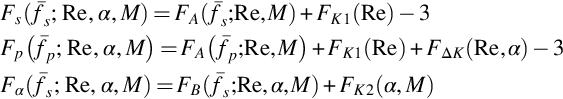
The function FK1 sets the level of the model spectrum FA and has the form

FΔK provides an additional adjustment to the level of the model spectrum for the pressure side contribution

where the group Reδp*/c is the Reynolds number based on the pressure side boundary-layer displacement thickness. For brevity we have not explicitly indicated functional dependence on δp*/c. Function FK2 sets the level of the model spectrum due to separation, FB, and is

where

The function FA defining the spectral shape and frequency scaling for attached flow is
where
For the separated flow portion the spectral shape and frequency scaling function FB is similarly defined as
where

Note that all angles are in degrees, and that these relations are valid for angles of attack from 0 to 12.5 degrees or γo, whichever is the smallest.
The above equations constitute a prediction method that accounts not only for Reynolds number and boundary-layer thickness effects but also for the most important aerodynamic parameter—the angle of attack. At the conditions of the BPM measurements, these formulae constitute a curve fit to their experimental data and can be used to illustrate some basic variations, as we have done in Figs. 15.7 and 15.8.
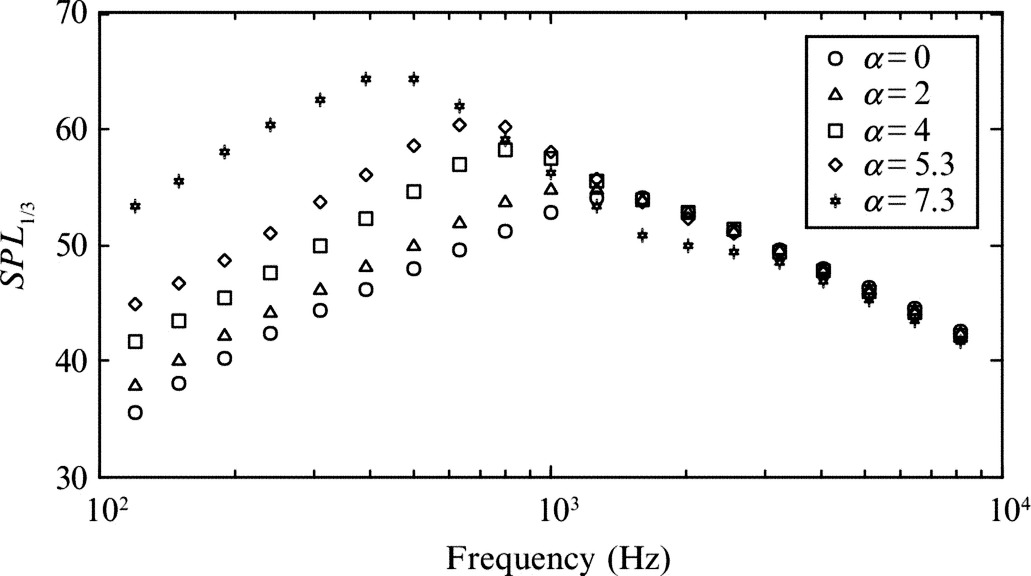
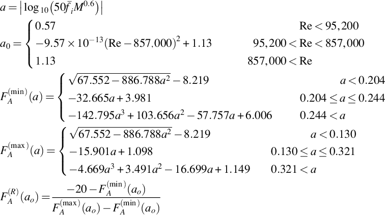
Fig. 15.7 shows the effect of angle of attack on the trailing edge noise radiated by a tripped 22.86 cm chord blade. Angle of attack has surprisingly little effect on the high-frequency portion of the spectrum. At low frequencies the sound level increases with angle of attack at an increasing rate, and the frequency at which the sound level reaches its maximum decreases by roughly a factor of 3 between 0 and 7.3 degrees. This change presumably reflects the effects of adverse pressure gradient on the suction-side boundary layer, increasing the scale and intensity of turbulent motions.
Fig. 15.8 shows the effect of chordlength on the sound at zero angle of attack. The obvious effect here is that as the chordlength is increased, the trailing edge boundary layer grows, and so the frequency of the sound drops, these effects being roughly in proportion. In Fig. 15.8 we have factored this variation out by plotting the sound against frequency normalized on chord and flow speed, as fc/U, where f is frequency in Hz. In this form we can see that the simple chord scaling just described works well at frequencies below fc/U≈5 (i.e., turbulent scales larger than about 20% of the chord). At higher frequencies the sound level increases with the chordlength because the greater the chordlength, the higher the Reynolds number of the boundary layer, and the greater the range and energy of the turbulence it produces at small scales.
Fig. 15.5 includes a prediction using the BPM method of the same NACA 0012 airfoil results compared with Amiet's method. The BPM prediction is also quite good, though curiously shows a larger difference at low frequencies. Trailing edge noise measurement at low frequencies is notoriously difficult, and the differences may reflect the fact that BPM include only noise contributions in antiphase across the chord line, whereas the measurements of [6] were made using a phased microphone array to distinguish trailing edge noise sources from one side of the airfoil.
A particular advantage of the BPM scheme is that it is not restricted to self-noise generated by turbulent boundary-layer flow over a sharp trailing edge. Self-noise generated by vortex shedding from a trailing edge (due to trailing edge bluntness or a laminar trailing edge boundary layer), stalled flow over the airfoil, and interaction of boundary-layer turbulence with the tip of a blade during the formation of a trailing vortex can be handled by essentially the same approach. BPM reviewed experimental data and present further curve fits that allow prediction of these sources and, in the case of laminar shedding noise and stall noise, the conditions at which these become the dominant self-noise mechanisms.
The BPM method is often used for airfoils that do not have a NACA 0012 section. This may be done by entering trailing edge boundary-layer thicknesses computed or measured on the airfoil in question and entering an angle of attack referenced to zero lift. It is also quite common to see predictions at conditions that exceed the range of the experiments on which the method is based. (BPM did so themselves on a model scale rotor in the DNW-LLF, as discussed in Appendix C of Ref. [8], which actually caused them to refine some of their prediction methods.) These approaches are fine for rough estimates, but it is important to remember that such extrapolations can lead to substantial error.
15.4 Roughness noise
We have seen above that the intense surface pressure fluctuations generated by a turbulent boundary layer are a significant source of sound at low Mach numbers when they are scattered from a trailing edge. Given the form of Curle's equation (4.3.9) one might be forgiven for thinking that turbulent boundary-layer flow over a smooth flat surface would be a similarly important source of noise. This is not the case. To see why, imagine the application of Eq. (4.3.9) to flow over an infinite rigid wall defined by the plane x2=y2=0, as shown in Fig. 15.9.
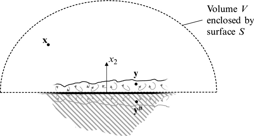
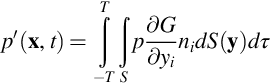
We apply this equation by taking the volume of integration V as existing only above the surface so that its enclosing surface S is formed by the wall and hemispherical surface of much greater radius than the extent of the flow and the turbulent boundary layer. Given that the velocities on the surface will be zero, because of the non-penetration and no-slip conditions, then Eq. (4.3.9) becomes

where the sound field has been written in terms of its pressure fluctuations, and pij is the sum of the pressure and viscous stresses pδij−σij. At low Mach number, the only significant viscous stresses acting on the wall are those associated with viscous shear parallel to the wall, σ12=σ21=μ∂v1/∂y2 and σ23=σ32=μ∂v3/∂y2. Thus, since nj=(0,1,0) the first term expands to give
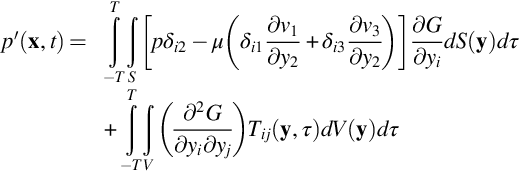
This equation can be evaluated in two ways, first using the free-field Green's function, Go, i.e.,
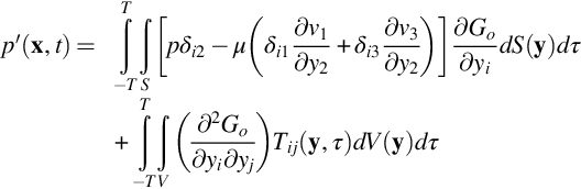
Alternatively, we can evaluate Eq. (15.4.2) using the tailored Green's function of Eq. (4.5.3) that accounts for sound reflection from a flat surface

where y#=(y1,−y2,y3) identifies locations of the image sources in the wall. As indicated, this function is merely the sum of the free-field Green's function for the source and image points. Differentiation of Eq. (15.4.4) shows that on the wall at y2=0, ∂GT/∂y2=0, ∂GT/∂y1=2∂Go/∂y1, and ∂GT/∂y3=2∂Go/∂y3. So, substituting these relations into Eq. (15.4.2) we lose the pressure term and obtain

By comparing Eqs. (15.4.3), (15.4.5) we see that effect of the surface pressure term is equivalent to a doubling of the viscous shear stress dipole and the addition of a quadrupole term representing the noise made by the image of the boundary-layer turbulence in the wall. The shear dipole is expected to be negligibly weak except perhaps at low Reynolds numbers, and even then it has been argued [9] that this term is not a true source but acts as a modifier to the propagation of acoustic waves adjacent to the surface. The quadrupole term is, of course, small in any low Mach number flow.
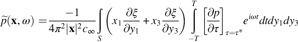
The relative silence of turbulent boundary layers is not maintained when the wall is rough (Fig. 15.10). In this case the unsteady boundary-layer pressure field is experienced on an uneven surface so that individual features of the roughness (which we will refer to as roughness elements) are subjected to an unsteady pressure force tangential to the wall that acts as a dipole source, radiating sound back out into the flow. This source is enhanced by the effect that the roughness has on the boundary layer itself, intensifying the turbulence and the associated surface pressure fluctuations. To analyze this situation, we begin once more with Eq. (15.4.1) but without the viscous and Lighthill stress tensor terms
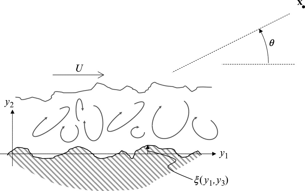
As shown in Fig. 15.10, we define our coordinates so that the mean plane of the wall is at y2=0 and with the surface shape defined by the function ξ so that on the surface y2=ξ(y1,y3). Note that we are assuming that ξ is single valued function, i.e., the surface has no overhanging elements. The apparently complex task of evaluating the derivative of the Green's function on the rough surface is simplified by using once more the tailored Green's function of Eq. (15.4.4). Since ∂G/∂y2=0 at y2=0 we can write the derivatives of this Green's function at the rough surface in terms of the Taylor series expansions
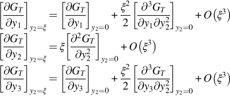
Substituting Eq. (15.4.4) into Eq. (15.4.7), and ignoring all but the leading order terms, we obtain
Where these results have been simplified using far-field approximations. For example, the result for ∂GT/∂y1 without simplification is

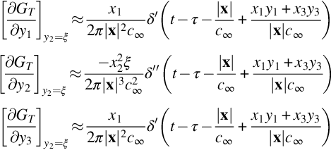
In the far-field x is large (using an origin close to the source), so we can neglect the second term compared to the first, ignore y1 relative to x1 in the remaining numerator, and replace |x−y|2 in the remaining denominator by |x|2 and |x−y| in the argument of δ′ by |x|−xiyi/|x|, thereby giving the result in Eq. (15.4.8). Substituting Eq. (15.4.8) into Eq. (15.4.6) we obtain
where

Performing the time integration then yields

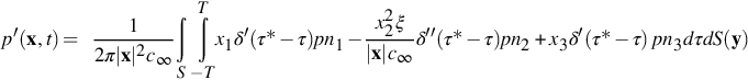
where dS and ni represent the surface area and unit outward normal on the uneven rough wall. As shown in Fig. 15.11 these can be expressed in terms of the roughness height function ξ as

and so,

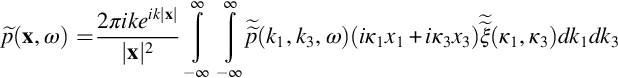
The two terms inside the integral are not of the same order. If we characterize the timescale of the flow in terms of the turbulence lengthscale L divided by the flow velocity U and denote the characteristic height of the roughness as h, then the second term is smaller than the first by a factor of MLξ/L, where Lξ is the streamwise or spanwise scale of the roughness. The second derivative term thus scales as if it were a quadrupole, and we neglect it as we have already neglected the quadrupole turbulence sources. Taking the Fourier transform of the result with respect to observer time we obtain
Changing the variable of time integration to τ*, and remembering that taking the time derivative of a variable is equivalent to multiplying its Fourier transform by −iω, we obtain
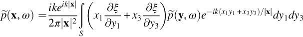
where k is the acoustic wavenumber ω/c∞. From the definition of the inverse spatial Fourier transform, we can express ![]() in terms of the wavenumber frequency transform of the wall pressure
in terms of the wavenumber frequency transform of the wall pressure ![]() as
as

giving

where
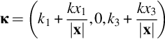
The inner integral of Eq. (15.4.17) has the form of a wavenumber transform. Indeed, if we introduce the wavenumber transform of the surface height,
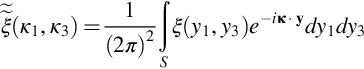
and note that ![]() and
and ![]() are the wavenumber transforms of the surface slopes in the y1 and y3 directions, then Eq. (15.4.17) can be reduced to
are the wavenumber transforms of the surface slopes in the y1 and y3 directions, then Eq. (15.4.17) can be reduced to
This is the equation for the roughness noise. If the features of the roughness are acoustically compact in all directions so that k≪k1 and k≪k3, then κ1 and κ1 are indistinguishable from k1 and k3.
For Eq. (15.4.19) to be practically useful, we need to express the far-field sound in terms of its frequency spectrum
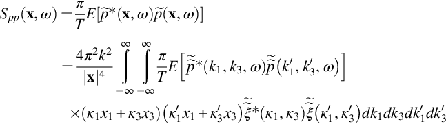
Now, if we assume that the portion of the fluctuating surface pressure field that is responsible for the roughness noise is homogeneous then we can write the expected value in the integral in terms of the wavenumber spectrum of the surface pressure Φpp. Note that this assumption excludes pressure fluctuations directly associated with the individual flows around roughness elements, such as due to the local effect of eddy shedding from an element or the interstitial flows between adjacent elements. From Eq. (8.4.37), we have
and so,

Eq. (15.4.21) is an expression for the sound field that assumes that we know the precise roughness geometry. In many situations it is more likely that we will only have statistical knowledge of the roughness, and for this situation the expected value operator on the right-hand side of Eq. (15.4.20) needs to encompass the surface coordinate terms as well as the pressure terms. Assuming there is direct correlation between the details of the pressure field and those of the rough surface (which is inevitable if the homogeneity assumption is valid) then the result of this derivation becomes

where Σ is the area of the surface, projected onto the y2=0 plane, h is the RMS roughness, and
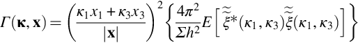
Note that the term inside the curly braces is the wavenumber spectrum of the surface height, normalized on its mean square. We see that both Eqs. (15.4.21), (15.4.22) cleanly separate the flow-dependent acoustic source term, represented by the surface pressure wavenumber spectrum, from the surface geometry term representing the spectrum of the surface slope in the direction of the observer.
These equations provide perfectly practical expressions for roughness noise prediction if we know the surface geometry, or its typical statistical form, and the boundary-layer parameters needed to define one of the wavenumber frequency spectrum models of the surface pressure, such as Eq. (9.2.34) or (9.2.38). Given the fact that we have neglected sound generated by the individual flows around roughness elements, we might expect these equations only to be accurate when the roughness comparable to the viscous scales of the boundary layer and such flows are suppressed. However, this is not the case and accurate predictions have been made in flows where the roughness elements are at least as large as the displacement thickness [10]. The implication is that the scattering of the homogeneous components of the surface pressure spectrum is a much greater contributor to roughness noise than the self-noise of individual elements. For a broadband rough surface, the predicted far-field sound has been found to be only weakly dependent on the form of the wavenumber frequency spectrum [10], so the exact choice or accuracy of this model is not likely to be critical in most circumstances.
As regards the scaling implicit in Eq. (15.4.22), we expect that k˜M/L, that the wavenumber spectrum of surface pressure will vary approximately as ρo2U4S(ω)L2, where L represents the scale of the turbulence, and that the wavenumbers k1 and k3 (and κ1 and κ3) representing flow scales will vary as 1/L. We thus have, for an observer above the mid-span of the surface (x3=0),
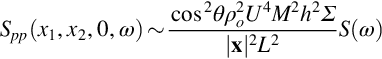
where we are taking κi≈ki and introducing cos θ=x1/|x| and S(ω), with units of seconds, which gives the normalized spectral shape. This shows that roughness noise has classical dipole scaling and directivity, the dipole being oriented parallel to the wall. The sound increases in proportion to the area of the surface and the square of the height of the roughness elements. Dividing Eq. (15.4.24) by Eq. (15.2.13) for trailing edge noise and ignoring the differences in spectral shape and directivity gives
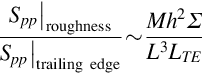
Since h/L is likely to be small, we see that at low Mach number roughness noise will be the dominant self-noise source only when the surface area of the roughness is very large compared to the product of the turbulence scale and the total edge length. This happens with undersea vehicles, for example, which can have large surface area but small lifting surfaces. Roughness noise can also be important in determining the acoustic noise floor of wind tunnels [11], where an observer in a hard-wall test section finds themselves far from any edge sources, but in the direct line of streamwise roughness noise dipoles associated with the walls of the diffuser and contraction.
The above scaling argument ignores factors controlling the shape of the noise spectrum. From Eq. (15.4.22) we see that the observer hears a sound spectrum whose shape is determined by wavenumber filtering of the surface pressure fluctuation field, the filter being the surface slope spectrum represented by Γ. For rough surfaces with random roughness elements defined by near-vertical sides it can be shown [12] that the slope spectrum is wavenumber white, i.e., Γ is simply a constant. In this case, Eq. (15.4.22) becomes dependent on the unweighted wavenumber spectrum integrated with respect to k1 and k3, which is simply equal to the wall pressure frequency spectrum, i.e.,

Thus the roughness noise spectrum normalized on the surface pressure frequency spectrum should simply be proportional to the frequency squared, the mean square roughness height, and the area of the rough surface, i.e.,
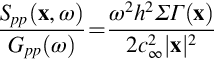
Fig. 15.12 shows this type of behavior on roughness noise measurements made over a series of sandpaper surfaces of different grit size [13]. The smallest grit size of 100 implies roughness elements with heights comparable to the viscous sublayer thickness, whereas the largest, of 20, indicates roughness elements that penetrate into the log layer and are comparable to the displacement thickness. The sound spectra are normalized on the surface pressure frequency spectrum and the square of the roughness height and convincingly follow a line proportional to ω2, except at high frequencies for the largest roughness sizes.

Sandpaper and other stochastic surfaces do not strictly have wavenumber white surface slope spectra, but their slope spectra are expected to have a broad maximum. In the vicinity of this maximum not only Γ is approximately constant, but the surface pressure wavenumber spectrum is most heavily weighted by Γ, making it probable that this portion of the integral in Eq. (15.4.22) will dominate what is heard in the far field. Thus Eq. (15.4.27) provides a simple means of estimating the roughness noise spectrum generated by many random surfaces.
The fact that the rough surface acts as a filter on the surface pressure field in determining the far-field sound raises the intriguing possibility of using such a surface as a probe. That is, designing a deterministic surface with a shape chosen to reveal a specific part of the surface pressure wavenumber frequency spectrum in the noise it radiates. For example, consider a wall with sinusoidal ribs of wavenumber ![]() . The shape of the wall is
. The shape of the wall is
which has the wavenumber transform
Substituting this into Eq. (15.4.19) and assuming that the surface is acoustically compact, so that κ=k, we obtain

So that the far-field sound spectrum is
Note that if our coordinate system is oriented so that k1 is measured in the flow direction, then the wavenumber frequency spectrum at negative k1(w) will be negligible since this implies upstream traveling turbulence, and we can truncate this result to

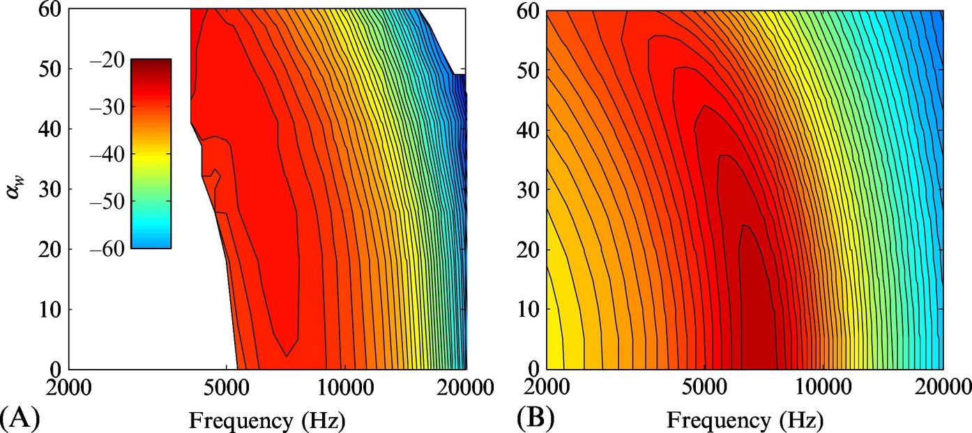
So, a sinusoidal surface of wavenumber k(w) radiates only the portion of the wavenumber frequency spectrum of the wall pressure at that wavenumber. The shape of the far-field sound spectrum gives the frequency dependence or the surface pressure spectrum at that wavenumber, multiplied by ω2. By turning a sinusoidal surface to different angles, different parts of the wavenumber frequency spectrum can be revealed. Fig. 15.13 illustrates just how this works. The wavenumber frequency spectrum of the wall pressure is represented in terms of contour surfaces drawn using the Chase model of Eq. (9.2.34). We are considering the sound radiated by a circular patch of sinusoidal ridges, with ridges oriented perpendicular to the direction αw where ![]() . This surface will radiate sound that reveals the shape of the wavenumber frequency spectrum along the line AA. By rotating the surface to vary αw we can reveal an entire cylindrical cut through the wavenumber frequency spectrum, as shown. Fig. 15.14 shows results from just such a measurement used to reveal the wavenumber spectrum of a wall-jet boundary layer using a ridged surface with a 1.26-mm wavelength [14]. This is a far smaller wavelength (and thus higher wavenumber) that could be probed using an array of conventional surface microphones and is a much easier measurement, requiring only a single far-field microphone. The results (Fig. 15.14A) are plotted as a map, which reveals the convective ridge forming a near-vertical arc in the plot. This appears to be in fair agreement with the prediction of the map using the Chase model (Fig. 15.14B).
. This surface will radiate sound that reveals the shape of the wavenumber frequency spectrum along the line AA. By rotating the surface to vary αw we can reveal an entire cylindrical cut through the wavenumber frequency spectrum, as shown. Fig. 15.14 shows results from just such a measurement used to reveal the wavenumber spectrum of a wall-jet boundary layer using a ridged surface with a 1.26-mm wavelength [14]. This is a far smaller wavelength (and thus higher wavenumber) that could be probed using an array of conventional surface microphones and is a much easier measurement, requiring only a single far-field microphone. The results (Fig. 15.14A) are plotted as a map, which reveals the convective ridge forming a near-vertical arc in the plot. This appears to be in fair agreement with the prediction of the map using the Chase model (Fig. 15.14B).