1.1 Aeroacoustics of low Mach number flows

Sound is a fundamental part of human life. We use it for social interaction, for art, for communication and education, and for understanding each other. Sound is also a byproduct of human activities. Unwanted sound, or noise, can adversely affect our productivity, health, security, and quality of life. Flow noise generated by fans, vehicles, wind turbines, and propulsion systems are major contributors to this unwanted sound. Aeroacoustics is the study of noise generation by air flows, and the way in which aerodynamic systems can be designed to minimize noise.

Much of our motivation for understanding flow generated noise originates from the aircraft industry. Regulations require noise certification for all new aircraft and so new products must meet increasingly high standards for noise emissions. Historically, most key developments can be traced to the advent of the jet engine at the end of World War II and its role in ushering in a new era in commercial air transportation. The original engines were unacceptably loud and it was clear that for the jet engine to be viable the noise had to be reduced. At that time there was no understanding of how sound waves could be generated by a turbulent flow, although theories did exist for sound radiation from vibrating surfaces, and even propellers. In 1952 Sir James Lighthill [1] published his theory of aerodynamic sound and the subject of aeroacoustics was born. This theory, which is known as Lighthill's Acoustic Analogy, provides the basis for our understanding of sound generation by flow. It is an exact re-arrangement of the equations of fluid motion, but has certain limitations, which must be carefully understood if it is to be applied correctly. Lighthill's theory has been frequently challenged, but remains the most important and effective analytical tool for the understanding and reduction of flow noise.

The purpose of this book is to provide an introduction to the basic concepts that describe the sound radiation from low Mach number flows, in particular flows over moving surfaces, which are the most widespread cause of flow noise in engineering systems. This includes fan noise, rotor noise, wind turbine noise, boundary layer noise, airframe noise, and aircraft noise, with the exception of jet and shock associated noise. The basic principles are also applicable to hydroacoustics, the study of flow generated noise in underwater applications. The primary difference between aero and hydroacoustics is that water is an almost incompressible fluid and thus usually involves Mach numbers that are an order of magnitude smaller than in aerodynamic applications.

This book is intended to be an introductory text on low Mach number aeroacoustics for graduate students who do not have a background in acoustics but who are familiar with the mathematical foundations of fluid dynamics and thermodynamics. It is written in four parts. Part 1 introduces the fundamentals, including the basic equations of unsteady fluid flow, a review of fluid dynamics concepts, and an introduction to linear acoustics. Lighthill's acoustic analogy is then introduced, leading to Curle's theorem, the Ffowcs Williams and Hawkings equation, the linearized Euler equations, vortex sound, and a discussion of turbulence and turbulent flows. This is followed by Part 2 that details experimental measurement techniques, including the use of microphones and flow measurement devices, signal processing and phased arrays, and wind tunnel testing methods. Part 3 of the text deals with edge and boundary layer noise including leading edge noise, trailing edge noise, and the flow over rough surfaces. Finally, Part 4 considers rotating sources such as fans, propellers, and rotors. It includes chapters on open rotor noise, duct acoustics, and fan noise.

1.2 Sound waves and turbulence

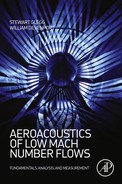
Sound waves cause small perturbations in pressure that propagate through a fluid medium. The speed of propagation, c_o, depends on the local properties of the fluid, but is typically about 343 m/s in air and 1500 m/s in water. The simplest form of a sound wave is a harmonic wave that has a sinusoidal variation in space with a wavelength λ and a frequency f=c_o/λ, Fig. 1.1. The human ear responds to frequencies between 20 Hz and 20 kHz, so typical wavelengths of interest are from 17 m to 17 mm in air.

In contrast, turbulence is caused by instabilities in viscous shear flows breaking down into random chaotic motion. Common examples are boundary layers on wings and aircraft fuselages, and the wakes behind moving vehicles. At higher speeds (high Reynolds number) the loss of energy due to turbulent mixing far exceeds the loss that occurs directly from viscous action. Turbulence is sometimes conceptualized as if it consisted of eddies convected at constant velocity through the medium without evolving in the convected frame of reference. This simplification is known as Taylor's hypothesis and the average convection speed U_c is typically taken to be about 60–80% of the free stream velocity. The size of the eddies L is usually the same order of magnitude as the smallest dimension of the mean flow, for example the boundary layer, shear layer, or wake thickness.

When convected turbulence encounters a solid body, it generates rapid changes of pressure on the surface of the body that radiate as sound waves through the fluid. The frequencies of the fluctuations which result from this type of interaction are determined by the eddy size and its convection velocity, and can be estimated as f≈U_c/L. The sound waves generated at this frequency will therefore have a wavelength λ≈Lc_o/U_c. In low Mach number applications, the convection speed is always much less than the speed of sound (U_c≪c_o), so the acoustic wavelength is always much larger than the size of the eddies generating the sound. The disparity in scales between the turbulent eddy dimensions and the acoustic wavelength is one of the most important features of aeroacoustics and hydroacoustics and one of the reasons that the subject is so challenging.

1.3 Quantifying sound levels and annoyance

The ear responds to the pressure fluctuations of sound waves to cause the sensation of hearing. When carrying out calculations of noise levels and designing for quiet systems it is always important to keep in mind the end goal. This is most often the level of annoyance experienced by a human listener.

The human ear has a remarkable dynamic range and can hear sound waves with amplitudes as low as 20 μPa and as high as 200 Pa before encountering the threshold of pain. The ear's sensitivity is logarithmic and so sound is measured using a decibel scale, referred to as the sound pressure level (SPL). This is given in terms of the root mean square of the fluctuating pressure time history p_rms and a reference pressure p_ref as

$\mathrm{S}\mathrm{P}\mathrm{L}=20{log}_{10}\left(p_{rms}/p_{ref}\right)$

where the units are stated as dB(re p_ref). It is important to specify the reference sound pressure p_ref when quoting a result in decibels because different units are used in different applications. For almost all airborne applications the standard is p_ref=20 μPa, but results in underwater applications are not as well standardized. The most common reference pressure used in underwater acoustics is p_ref=1 μPa, but historical data is also given in other units such as p_ref=1 μbar.

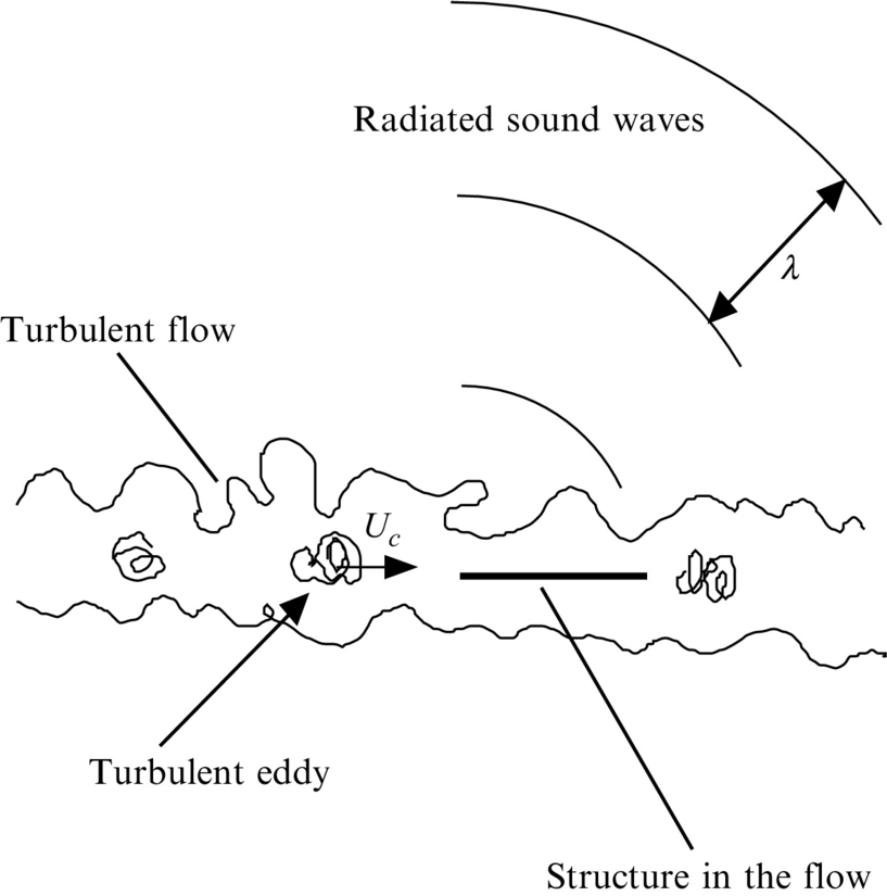
The root mean square pressure p_rms is the time average of the square of the fluctuating pressure. At any instant the pressure at a point is given as the sum of the mean background pressure p_o and a time varying perturbation p′(t). If p(t) is the pressure at a point in the fluid then the pressure perturbation is $p^{\prime }\left(t\right)=p\left(t\right)-p_o$. The root mean square or “rms” pressure is then defined as

$p_{rms}=\sqrt{\frac{1}{2T}{\displaystyle {\int }_{-T}^T{\left(p\left(t\right)-p_o\right)}^{2}dt}}$

where the averaging time must be large enough to include many cycles of the lowest frequency contained in the signal.

The human ear also discriminates the frequency of sound in a logarithmic manner. The frequency content of noise is therefore often characterized by summing up the sound into one-third octave bands that appear as equal intervals on a logarithmic scale. In acoustics, an octave is a doubling of the frequency and thus a third-octave band integrates the sound over a band for which the upper limit is 2^1/3 times its lower limit. The mid-band frequencies in Hertz are given by the relation

$f_n=1000\times 2^{\left(n-30\right)/3}$

where n is known as the band number [2]. Thus the band extends from f_n×2^−1/6 to f_n×2^1/6.

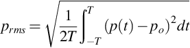
The typical response of the ear at different frequencies is plotted in Fig. 1.2 and we see that low and high frequencies are significantly less important than the mid-frequency range around 1 kHz. Note especially how the ear does not respond well to frequencies below 100 Hz, although sometimes low-frequency sounds are identified as being most irritating. To obtain a measure of the perceived loudness of a sound the most commonly used metric is the dB(A) level. This applies a weighting to each one-third octave band level and then each band level is summed on an energy basis. Since the dB(A) level corrects for the sensitivity of the ear, and is easy to measure directly using a sound level meter, it is used extensively in noise control applications. It has also been found to be a good measure of annoyance and so most noise ordinances are defined using this unit with corrections for duration, pure tones, and day/night levels. Other measures of annoyance such as perceived noise level (PNL) and effective perceived noise level (EPNL) are used in assessing aircraft noise.

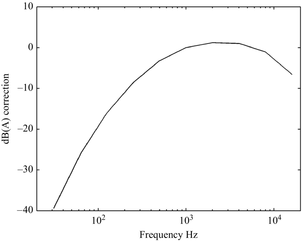
It is important to appreciate that simple physical scaling of sound levels from model scale tests to full scale applications must also incorporate a correction that accounts for annoyance. For example, slowing the rpm of a propeller will not only reduce its source level, but will generate lower frequencies which receive a larger negative A-weighting correction. The dB(A) level will therefore scale quite differently from the SPL, and significant additional noise benefits can be achieved by changing the frequency content of a sound.

In this text we will not attempt to rate noise source levels in subjective units such as dB(A), PNL, or EPNL, but rather the focus will be on the fundamental physics behind the sound generation process. However, it is important to keep in mind that based on the sensitivity of the ear (Fig. 1.2), the frequencies of most concern to humans usually lie between about 350 and 10,000 Hz. This roughly corresponds to wavelengths between 1 m and 3 cm in air.

1.4 Symbol and analysis conventions used in this book

While there is no universally agreed upon nomenclature for aeroacoustics, we use symbol conventions that will be familiar to many aeroacousticians. In this way analysis methods or results described in this book will be, as far as possible, recognizable when seen elsewhere in the aeroacoustics literature. We have also strived to be as consistent as possible and avoid using the same symbol for quantities that may be confused. Recognizing that these desires often conflict with that of familiarity, we have included in Appendix A both a list of symbols for basic quantities that appear repeatedly throughout the book, as well as a chapter-by-chapter nomenclature for more specialized symbols.

Our conventions for symbol modifiers are also listed in Appendix A and the most important ones are summarized here. Vector quantities are represented using bold symbols, such as x for position, or using subscript notation to refer to their Cartesian components, e.g., x₁, x₂, and x₃. Except in special cases, the mean part of a variable will be denoted by subscript “o” or an overbar, the latter being used to indicate an averaging or expected value operation. The fluctuating part (such as p′(t) discussed above) will usually be denoted using a prime. A tilde accent, such as $\tilde{p}\left(\omega \right)$ is used to denote the Fourier transform of the variable in question with respect to time, whereas a caret accent, such as $\hat{p}$ denotes the complex amplitude of a signal with harmonic time dependence.

Fourier transforms are perhaps the most important mathematical tool of aeroacoustic analysis. Except where otherwise noted we define the Fourier transform of a time history as

$\tilde{p}\left(\omega \right)=\frac{1}{2\pi }{\displaystyle {\int }_{-T}^T{p}^{\prime }\left(t\right)e^{i\omega t}dt}$

where T tends to infinity, and the inverse Fourier transform as

$p^{\prime }\left(t\right)={\displaystyle {\int }_{-\infty }^{\infty }\tilde{p}\left(\omega \right)e^{-i\omega t}d\omega }$

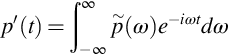
where ω is angular frequency and we are using the symbol i to represent the square root of −1. We define the one-dimensional Fourier transform of a variation over distance as

$\stackrel{\approx }{f}\left(k_1\right)=\frac{1}{2\pi }{\displaystyle {\int }_{-R_{\infty }}^{R_{\infty }}f\left(x_1\right)e^{-i{k}_1{x}_1}d{x}_1}$

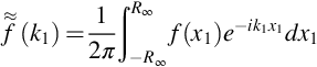
where R_∞ tends to infinity, and the inverse transform as

$f\left(x_1\right)={\displaystyle {\int }_{-\infty }^{\infty }\stackrel{\approx }{f}\left(k_1\right)e^{i{k}_1{x}_1}d{k}_1}$

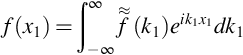
with two- and three-dimensional forms that are the result of repeated application of Eqs. (1.4.3) or (1.4.4). Here k₁ is the wavenumber. Note that in the forward time transform the exponent is positive, and the transformed variable is identified with a tilde, whereas it is negative in the forward spatial transform, and the transformed variable is identified with a double tilde.

It is important to realize that the above Fourier transform definitions are not universal to aeroacoustics analysis since there is no common standard. Our definitions are consistent with the definitions used in the previous aeroacoustics texts by Goldstein [3], Howe [4], and Blake [5]. Other texts on aeroacoustics, such as Dowling and Ffowcs Williams [6], and books focused on related topics, such as signal analysis [7], use different conventions, and it is obviously important to be aware of these distinctions when applying or comparing results.