Nomenclature

A.1 Symbol conventions, symbol modifiers, and Fourier transforms

Vectors are denoted using a bold character, such as x for position vector, or in terms of their Cartesian components, e.g., x₁, x₂, x₃, or x_i. Tensors are denoted in terms of their Cartesian components using double subscript notation, for example, p_ij for the compressive stress tensor.

In general, the mean value of a variable is denoted using subscript “o” (as in the mean pressure, p_o), or using the expected value operator denoted as E[ ] or using an overbar (as in the mean square pressure fluctuation, $\bar{{p^{'}}^{2}}$ $\bar{{p^{'}}^{2}}$ ). The fluctuating part of a variable is indicated using a prime, as in the fluctuating density ρ′=ρ−ρ_o. For some common variables special symbols are defined for the mean and fluctuating parts that do not follow these conventions. For example, U_i and u_i for the mean and fluctuating velocity components, respectively. The estimated value of a variable or statistic (used in discussing measurements) is indicated by triangular brackets, as in the estimated value of the mean square velocity fluctuation $〈\bar{u_{1}^{2}}〉$ $〈\bar{u_{1}^{2}}〉$ . The dot accent is used to indicate partial derivative with respect to time, as in the time rate of change of velocity potential, $\dot{ϕ}$ $\dot{ϕ}$ .

In certain situations, most notably Lighthill's analogy, variations in the thermodynamic variables are properly referenced to their ambient values indicated using an infinity subscript, for example ρ_∞. In these circumstances, the prime is used to indicate variation from the ambient value, e.g., ρ′=ρ−ρ_∞. The text has been written to make clear which meaning of the prime is intended whenever the distinction is significant.

The complex amplitude is indicated using a caret accent, as in the pressure amplitude of a harmonic wave $\hat{p}$ $\hat{p}$ where $p^{'} = \hat{p} e^{- i ω t}$ $p^{'} = \hat{p} e^{- i ω t}$ . The time Fourier transform is indicated using a tilde accent, and a wavenumber transform is indicated using a double tilde accent. We repeat here the Fourier transform definitions used in this book (also given in Chapters 1 and 3) for easy reference. Specifically, we define the Fourier transform of a time history as

$\tilde{p} (ω) = \frac{1}{2 π} \int_{- T}^{T} p^{'} (t) e^{i ω t} d t$ $\tilde{p} (ω) = \frac{1}{2 π} \int_{- T}^{T} p^{'} (t) e^{i ω t} d t$

si25_e

where T tends to infinity, and the inverse Fourier transform as

$p^{'} (t) = \int_{- \infty}^{\infty} \tilde{p} (ω) e^{- i ω t} d ω$ $p^{'} (t) = \int_{- \infty}^{\infty} \tilde{p} (ω) e^{- i ω t} d ω$

si26_e

where ω is angular frequency and we are using the symbol i to represent the square root of −1. We define the one-dimensional Fourier transform of a variation over distance as

$\overset{\approx}{f} (k_{1}) = \frac{1}{2 π} \int_{- R_{\infty}}^{R_{\infty}} f (x_{1}) e^{- i k_{1} x_{1}} d x_{1}$ $\overset{\approx}{f} (k_{1}) = \frac{1}{2 π} \int_{- R_{\infty}}^{R_{\infty}} f (x_{1}) e^{- i k_{1} x_{1}} d x_{1}$

si27_e

where R_∞ tends to infinity, and the inverse transform as

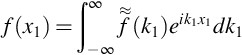
$f (x_{1}) = \int_{- \infty}^{\infty} \overset{\approx}{f} (k_{1}) e^{i k_{1} x_{1}} d k_{1}$ $f (x_{1}) = \int_{- \infty}^{\infty} \overset{\approx}{f} (k_{1}) e^{i k_{1} x_{1}} d k_{1}$

si28_e

with two and three dimensional forms that are the result of repeated application of the above two expressions. Here k₁ is the wavenumber in the x₁ direction. Note that in the forward time transform the exponent is positive, whereas it is negative in the forward spatial transform. Thus the four-fold Fourier transform of a quantity a( ) varying in space and time would be calculated as,

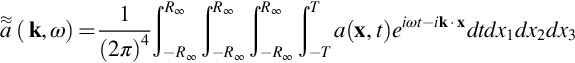
$\overset{\approx}{a} (k, ω) = \frac{1}{{(2 π)}^{4}} \int_{- R_{\infty}}^{R_{\infty}} \int_{- R_{\infty}}^{R_{\infty}} \int_{- R_{\infty}}^{R_{\infty}} \int_{- T}^{T} a (x, t) e^{i ω t - i k \cdot x} d t d x_{1} d x_{2} d x_{3}$ $\overset{\approx}{a} (k, ω) = \frac{1}{{(2 π)}^{4}} \int_{- R_{\infty}}^{R_{\infty}} \int_{- R_{\infty}}^{R_{\infty}} \int_{- R_{\infty}}^{R_{\infty}} \int_{- T}^{T} a (x, t) e^{i ω t - i k \cdot x} d t d x_{1} d x_{2} d x_{3}$

si29_e

In other texts or fields of study the convention used for the fourfold Fourier transform is often different. Most importantly some more mathematically oriented texts, such as the book by Noble [1] on the Weiner Hopf Method, the exponent +iωt+ik·x is used, and the factors of 2π may be shifted to the inverse transform, or replaced by √2π in both the transform and inverse transform. The final results of any derivation may of course be used to obtain the results in another convention by changing the sign of k (or ω or multiplying by factors of 2π, etc.). However, some care needs to be exercised if the result includes a multivalued function for which a branch cut has been defined, such as in the results presented in Chapter 13.

A.2 Symbols used

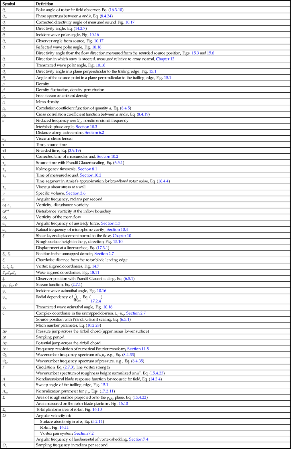
Symbols used are tabulated below in alphabetical order with Roman symbols listed before Greek symbols, and lower-case characters before upper case.

Symbol	Definition
a	Distance, representing;
	Airfoil semichord
	Radius of small sphere, Sections 3.4 and 3.5
	Streamwise spacing between shed vortices, Section 7.4
	Duct outer radius, Fig. 17.2B
	Amplitude of undisturbed gust, representing;
	Velocity, Eq. (6.3.4)
	Velocity potential, Eq. (13.4.1)
b	Distance representing;
	Span
	Duct inner radius, Fig. 17.2B
b, b_j	Spectral densities of the output of a phased array at the jth focus point, Eqs. (12.2.7), (12.3.4)
c	Airfoil chord length
c	Local unsteady speed of sound
c_m	Weighting function, Chapter 12
c_n	Fourier coefficients of sound from a rotor blade, Eq. (16.3.5)
c_o	Speed of sound
c_p	Specific heat at constant pressure
c_v	Specific heat at constant volume
c_∞	Free stream or ambient sound speed
d	Distance, representing;
	Semispan
	Distance between monopole sources
	Radial position of line vortex, Section 7.2
	Cylinder diameter, Section 7.4
	Pinhole diameter, Section 10.4
	Source separation, Fig. 12.4
	Chordwise blade displacement, Fig. 18.4
e	Specific internal energy
e	Viscous force per unit mass
e_T	Specific total energy
f	Frequency in Hz
f(r)	Longitudinal correlation function of homogeneous turbulence, Section 9.1
f(x,t)	Scalar function defining a surface, Section 5.1
f_i	Rotor blade surface loading per unit area, Section 16.2.1
${\bar{f}}_{i}$ ${\bar{f}}_{i}$	Normalized frequency 2πωδ_i⁎/U, Eq. (15.3.2)
f_n	Third octave band mid-band frequency
f_s	Sampling frequency
g(r)	Lateral correlation function of homogeneous turbulence, Section 9.1
g⁽¹⁾	First order leading edge blade response function, Eq. (13.4.5)
g⁽¹⁺²⁾	Second order leading edge blade response function, Eq. (13.4.6)
g_te	Trailing edge blade response function, Eq. (13.3.9)
h	Specific enthalpy
	Distance, representing
	Off center position of shed vortex, Section 7.4
	Off chord position of incident vortex, Section 7.5
	Test section height, Section 10.1
	x₂ distance between source and shear layer, Section 10.2, Fig. 10.17
	Cavity depth, Section 10.4
	Perpendicular distance from source to array, Fig. 12.4
	Vortex-blade separation, Fig. 14.7
	Root-mean-square roughness height, Eq. (15.4.22)
	Rotor blade thickness, Chapter 16
	Cascade blade spacing, Fig. 18.5
h_i	Initial length of material volume i
h_o	Mean specific enthalpy
h_∞	Free stream specific enthalpy
i	Square root of −1
i, j, k	Unit vectors in directions x₁, x₂, x₃
k	Acoustic wavenumber
k	Turbulence wavenumber magnitude, Section 9.1
k^(o)	Acoustic wavenumber vector in the direction of the observer, Eq. (4.7.8)
k^(w)	Wavenumber vector of sinusoidal ribs (k₁^(w),0,k₃^(w)), Eq. (15.4.28)
k, k_i	Wavenumber vector
k₁^(o)	Streamwise acoustic wavenumber with Prandtl Glauert scaling, Eq. (6.5.6)
k₁₃	$\sqrt{k_{1}^{2} + k_{3}^{2}}$ $\sqrt{k_{1}^{2} + k_{3}^{2}}$
k₃^(o)	Spanwise acoustic wavenumber with Prandtl Glauert scaling, Eq. (6.5.6)
k_e	Wavenumber scale of the largest eddies, Eq. (9.1.9)
K_n( )	Modified Bessel function of the second kind of order n
k_o	Acoustic wavenumber with Prandtl Glauert scaling, Eq. (6.5.6)
l_p(ω)	Frequency-dependent spanwise pressure lengthscale, Eq. (15.2.12)
m	Azimuthal mode order, Eq. (17.2.2)
n, n_i	Surface normal unit vector
n, n_i	Unit vector normal to a streamline in two dimensions, Fig. 6.3
n	Radial mode order, Section 17.2.2
n^(o), n_j^(o)	Unit outward normal vector
p	Pressure
p	Vector of Fourier transforms of measured microphone signals, Eq. (12.2.15)
p′	Pressure fluctuation, pressure perturbation
$\hat{p}$ $\hat{p}$	Complex amplitude of the acoustic pressure
p_bl	Boundary layer pressure fluctuation in the absence of the trailing edge, Section 15.2
p_c	Corrected sound pressure, Section 10.2
p_i	Incident acoustic pressure
p_ij	Compressive stress tensor, pδ_ij−σ_ij
p_m	Measured sound pressure, Section 10.2
p_o	Mean pressure
p_ref	Reference pressure
p_rms	Root mean square pressure
p_s	Scattered acoustic pressure, Section 3.5
p_t	Sound pressure just after refraction, Section 10.2
p_∞	Free stream or ambient pressure
q, q_n	Time Fourier transform of effective source strengths, Eq. (12.2.2) and Section 12.2.7, diagonal elements of B
q_m	Radial phase function, Eq. (17.6.3)
r	Radial coordinate, radial distance
r_c	Corrected propagation distance of measured sound, Fig. 10.17
r_e	Observer radius with Prandtl Glauert scaling, Eq. (6.5.5)
r_g	Source to observer distance with Prandtl Glauert scaling, Eq. (6.5.3)
r_m	Observer distance from source, Fig. 10.17
r_o	Distance to flow origin in distortion example, Section 6.3
r_o	Distance from source to array center, Chapter 12
r_r	Distance from the retarded source position to the observer, Figs. 15.3 and 15.6
r_y	Distance of the source point from the trailing edge, Fig. 15.1
s	Specific entropy
	Distance traveled by shed vortex, Section 7.4
	Laplace transform frequency, Chapter 13
	Blade index number, Chapter 18
	Blade spacing, Fig. 18.4
s	Unit vector along a streamline in two-dimensions, Fig. 6.3
t	Time, observer time
t	Unit vector out of plane of flow of Fig.6.3, s×n
t_g	Observer time with Prandtl Glauert scaling, Eq. (6.5.1)
u	Scale of velocity fluctuation due to largest eddies, Section 8.1
u( )	Time varying convection speed of shed vortex during acceleration, Section 7.4
u^(∞), $u_{i}$ $u_{i}$ ^(∞)	Undisturbed gust velocity at the inflow boundary, Eq. (6.2.6)
u^(g)	Goldstein's velocity perturbation, Eq. (6.1.9)
u^(h)	Goldstein's composite velocity perturbation, Eq. (6.1.12)
u, u_i	Velocity fluctuation
u⁺	Mean velocity in boundary layer inner variables, Eq. (9.2.15)
u₂	Upwash velocity of gust, Eq. (14.1.7)
u_n	Surface normal velocity fluctuation
u_n	Velocity component in direction of separation distance, Section 9.1
u_o	Surface velocity of sphere, Eq. (3.4.1)
u_r	Velocity fluctuation in the direction perpendicular to the trailing edge, Fig. 15.1
u_s	Velocity component normal to direction of separation distance, Section 9.1
u_t	Velocity component normal to direction of separation distance and u_s, Section 9.1
u_η	Kolmogorov velocity scale, Section 8.1
u_τ	Friction velocity, Section 9.2.2
$\hat{v}$ $\hat{v}$	Complex amplitude of the acoustic velocity
v, v_i	Velocity vector
v_o	Amplitude of sphere oscillations, Section 3.4
v_r, v_θ	Polar velocity components aligned with the trailing edge, Fig. 15.1
w	Complex potential, Eq. (2.7.10)
w′	Complex velocity, Eq. (2.7.11)
w( )	Window function
w, w_i	Deviation of the velocity from $U_{i}^{(\infty)}$ $U_{i}^{(\infty)}$
${\tilde{\tilde{w}}}_{2}$ ${\tilde{\tilde{w}}}_{2}$	Planar wavenumber transform of u₂(y₁, 0, y₃), Eq. (14.1.10)
w_c′	Convection velocity in the mapped domain, Section 2.7
w_m^(j)	Array steering vector for microphone m and focus point j, Eq. (12.2.4)
w_o	Amplitude of step gust
x, x_i	Position, far-field position of observer
x	Axial duct coordinate, Fig. 17.2A
x′	Observer position in frame moving with uniform flow, Eq. (5.4.1)
x, x′	Cascade chordwise position, Fig. 18.5 and Fig. 18.7
$x_{2}^{+}$ $x_{2}^{+}$	Distance from the wall in inner variables, Eq. (9.2.15)
x_o	Downstream-pointing axial location, Fig. 18.1
y, y_i	Position, near-field position of source
y′	Observer position in frame moving with uniform flow, Eq. (5.4.1)
y, y′	Cascade blade-normal position, Fig. 18.5 and Fig. 18.7
y^(c)	Centroid of noise generating surface
y^(v)	Line vortex coordinate, Section 7.2
z, z_i	Position, moving coordinates, rotor blade based coordinates
z	Complex coordinate, x₁+ix₂, y₁+iy₂
z	Liner acoustic impedance, Section 17.3
z	Unit vector aligned with line vortex, Fig. 14.7
A	Acoustic wave amplitude, Eq. (3.3.1)
	Pinhole area, Section 10.4
	Wavenumber multiplier, Eq. (13.3.9)
A( )	Fourier transform of the scattered pressure, Eq. (13.2.7)
A₋( ), A₊( )	Half-range Fourier transforms of the scattered pressure, Eqs. (13.2.8), (13.2.9)
A_mn	Duct mode amplitude, Chapter 17
B	Integer factor used in frequency averaging, Section 11.6.1
	Parameter equal to $U_{c} / (c_{\infty} (1 - M^{2}))$ $U_{c} / (c_{\infty} (1 - M^{2}))$ , Eq. (15.2.11)
	Number of blades, Chapters 16 and 18
B	Matrix of estimated source auto and cross spectra from which the source image is extracted, Eq. (12.2.18)
B( )	Component function of the wavenumber transform of the scattered field, Section 13.2.2
C, C_mn	Cross-spectral matrix of microphone signals, Eqs. (12.2.8), (12.2.16)
C₋( ), C₊( )	Half-range Fourier transform of the gradient of the scattered pressure, Chapter 13
C_ab	Cospectrum between a and b, Section 8.4
C_d	Drag coefficient of 2D body
C_f	Friction coefficient $C_{f} ≡ τ_{w} / \frac{1}{2} ρ U_{e}^{2}$ $C_{f} ≡ τ_{w} / \frac{1}{2} ρ U_{e}^{2}$
C_L	Coefficient of fundamental of cylinder lift fluctuations
C_p	Nondimensional acoustic pressure due to loading noise, Eq. (16.2.5)
C_q	Nondimensional acoustic pressure due to thickness noise, Eq. (16.2.19)
D	Cavity diameter, Section 10.4
D( )	Fourier transform of the potential jump across a blade, Eq. (18.3.9)
D/Dt	Substantial derivative
D_o/Dt	Substantial derivative for convection with the mean flow
D_∞/Dt	Substantial derivative relative to uniform motion at U_∞ or $U_{i}^{(\infty)}$ $U_{i}^{(\infty)}$
E	Energy spectrum function of homogeneous turbulence
E[ ]	Expected value
E₂( )	Modified Fresnel integral function, Eq. (13.2.3)
F, F_i	Force on the fluid (imposed by an aerodynamic body for example)
F₂	Negative of the lift force on an airfoil
F₋( )	Laplace transform of the scattered field in the limit as the x₁ axis is approached from the positive side for x₁<0, Eq. (13.2.14)
F()	Array sensitivity function, Chapter 12
F₊( )	Laplace transform, with respect to x₁ of the scattered field in the limit as the x₁ axis is approached from the positive side for x₁>0, Eq. (13.2.13)
F_A, F_B, F_K1, F_K2, F_ΔK	Component parts of model trailing edge noise spectral forms F_i, Section 15.3
F_i	Model spectral forms for trailing edge noise spectra SPL_i, Section 15.3
F_D	Rotor blade drag force due to an element of its span ΔR
F_jn	Point spread function at focus point y_j due to a source at y_n, Eq. (12.2.11)
F_L	Rotor blade thrust force due to an element of its span ΔR
G	Green's function, G(x,t\|y,τ)
G	Matrix of source Green's functions, Eq. (12.2.15)
G₋(s), G₊(s)	Positive and negative range Laplace transforms of the x₂ gradient of the scattered field, in the limit as the x₁ axis is approached for x₁<0, Section 13.4.1
G_aa	Single sided time autospectrum of quantity a, Section 8.4
G_e	Green's function in the fixed frame with a free stream, Eq. (5.4.2)
G_g	Green's function with Prandtl Glauert scaling, Eq. (6.5.1)
G_o	Free field Green's function, Eq. (3.9.17)
G_o^#	Free field Green's function for image sources in the wall, Eq. (4.5.3)
G_T	Tailored Green's function, Section 4.5
H	Stagnation enthalpy
H	Distance in x₂ between source and observer, Fig. 10.17
H′	Stagnation enthalpy fluctuation
H( ), H_s( )	Heaviside step function
H_n⁽¹⁾( )	Hankel function of the first kind of order n
H_o	Mean stagnation enthalpy
I	Acoustic intensity vector E[(ρv)′H′], Eq. (2.6.16).
I	Integrated source level, Section 12.3.5
I_r	Radial component of the acoustic intensity vector
J_n( )	Bessel function of the first kind of order n
J₊(s), J₋(s)	Factorizations of γ, Eq. (13.2.16)
K₁	ω/U_c
L	Flow scale, representing
	Size of the eddies
	Lengthscale of the turbulence
	Scale of the mean flow distortion
	Vortex length
	Pinhole depth (Section 10.4), microphone array length (Chapter 12)
ℒ	Amiet's generalized lift function, Eq. (15.2.11)
L_eff	Effective pinhole depth, Section 10.4
L_f	Longitudinal integral scale, Eq. (9.1.4)
L_g	Lateral integral scale, Eq. (9.1.4)
L_ij	Integral scale of u_i in direction x_j, Eq. (8.4.29)
L_w	Wake half width, Section 9.2.1
L_w	Streamwise gust scale, Eq. (14.1.2)
M	Mach number
	Mass of fluid oscillating in pinhole
	Total number of array microphones, Chapter 12
M_r	Mach number in direction of observer
N_rec	Number of records used in spectral analysis, Chapter 11
P_o	Amplitude of pressure perturbation
Q	Acoustic monopole strength
Q, Q_i	Heat flux vector, Section 2.6.1
Q, Q_mn	Cross-spectral matrix of source strengths, Eq. (12.2.17)
$\hat{Q}$ $\hat{Q}$	Complex amplitude of the potential disturbance, Section 6.3
Q_ab	Quadrature spectrum between a and b, Section 8.4
Q_m,n	Fourier series components of the rotor noise source term, Eq. (16.3.15)
R	Gas constant
	Distance, representing
	Radius of circle, Section 2.7
	Distance from rotor axis, Fig. 16.11
	Radial distance from the duct axis, Fig. 17.2A
	Shear layer reflection coefficient, reflected over incident pressure amplitude
R_∞	Distance interval of Fourier wavenumber transform chosen such that −R_∞ to R_∞ encompasses the entire spatial variation
R_aa	Auto correlation function of quantity a, Eq. (8.4.3)
R_ab	Cross correlation function between a and b, Eq. (8.4.18)
Re	Reynolds number, see Section 2.3.2
Re_d	Cylinder diameter Reynolds number, Section 7.4
Re_θ	Boundary layer momentum thickness Reynolds number, Section 9.2.2
R_ij	Velocity correlation tensor, Section 8.4.3, Eq. (9.1.3)
R_n	Radius segment in Amiet's approximation, Eq. (16.4.4)
R_tip	Rotor tip radius
S	Surface, area
S( )	Sears function
S(ω)	Normalized spectral shape function, Chapter 15
S⁽¹⁾	Unsteady lift per unit span as a function of frequency, Eq. (14.1.4)
S_aa	Double sided time autospectrum of quantity a, Eq. (8.4.2)
S_ab	Cross spectral density between a and b, Eq. (8.4.20)
S_FF	Wavenumber frequency spectrum of the unsteady blade loading, Eq. (14.3.1)
S_o	Closed surface of integration in Ffowcs-Williams Hawkings equation, Section 5.1
SPL	Sound pressure level
SPL_i	One-third octave band spectra due to the suction (i=s) and pressure (i=p) side boundary layers, and angle of attack (i=α), Section 15.3
SPL_n	nth band of one-third octave sound pressure level, Eq. (8.4.9)
S_pp	Far-field sound frequency spectrum
St	Strouhal number
S_∞	Exterior surface of infinite volume, Section 5.1
T	Time period of Fourier frequency transform chosen such that −T to T encompasses the entire time history
	Time period of Green's function integration (−T to T), Eq. (3.9.8)
	Shear layer transmission coefficient, transmitted over incident pressure amplitude
T	Integral timescale, Eq. (8.4.5)
T_e	Temperature
T_ij	Lighthill stress tensor, Eq. (4.1.4)
T_o	Total sampling time
T_p	Rotor rotation period
T_v	Thrust disturbance timescale, Eq. (16.2.7)
U	Reference flow velocity
U, U_i	Mean velocity
U_∞	Nominal wind tunnel free stream velocity, Section 10.1
$U^{(\infty)}$ $U^{(\infty)}$ , $U_{i}^{(\infty)}$ $U_{i}^{(\infty)}$	Constant velocity vector of uniformly moving medium, Eq. (4.2.3)
U_c	Convection speed
U_e	Boundary layer edge velocity
U_o	Axial forward velocity of rotor, Fig. 16.11
U_r	Source velocity in direction of observer
U_s	Translational velocity of surface, Eq. (5.2.11)
U_s	Velocity of shear layer surface wave, Eqs. (10.2.3), (10.2.4)
U_w	Wake centerline velocity deficit, Section 9.2.1
U_∞	Free stream velocity
V	Volume
V	Number of stator vanes, Section 18.6
V, V_i	Velocity of moving surface, Eq. (5.1.12)
V_b	Blade velocity, Section 18.3.5
V_o	Volume exterior to S_o in Ffowcs-Williams Hawkings equation, Section 5.1
V_∞	Infinite volume, Section 5.1
W	Complex potential in the unmapped domain, Section 2.7
W′	Complex velocity in the unmapped domain, Section 2.7
W_a	Expected acoustic sound power output, Eq. (2.6.14)
W_c′	Convection velocity in the unmapped domain, Section 2.7
W_i	Uniform axial flow, Chapter 18
W_m	Array weighting for mth microphone, Chapter 12
W_s	Expected power generated due to steady contributions, Eq. (2.6.13)
W_T	Total power generated by a system, Eq. (2.6.11)
X₁, X₂, X₃	Drift coordinates, Eq. (6.2.1)
X_m	Axial dependency of ${\hat{ϕ}}_{m}$ ${\hat{ϕ}}_{m}$ , Eq. (17.2.4)
Y_i	Kirchoff coordinates (Eq. 7.3.3)
Y_m( )	Bessel function of the second kind of order m
α	Free-stream angle, angle of attack, angle of surface
	Wavenumber of the scattered pressure field in the x₁ direction, Eq. (13.2.4)
	Wavenumber parameter for duct acoustics, Eq. (17.2.8)
α′	Wind tunnel geometric angle of attack, Section 10.1
α_w	Orientation of ribs in the y₁y₃ plane, Fig. 15.13
β	$\sqrt{1 - M^{2}}$ $\sqrt{1 - M^{2}}$
β	Negative of the zero lift angle of attack for a Joukowski foil, Section 2.7
β_o	Location on the real axis of the inverse Laplace transform, Eq. (13.2.15)
β_o	Blade pitch angle, Fig. 16.22
β_a	Nondimensional liner admittance, Eq. (17.3.5)
χ_mn	Cut off ratio, Eq. (17.2.17)
χ_o	Angle between wake and stator-relative flow direction, Fig. 18.11
θ_s	Angle between wake and duct axis, Fig. 18.11
δ	Boundary layer thickness
δ( )	Dirac delta function, Eq. (3.9.3)
δ(x)	Dirac delta function (3D), Eq. (3.9.4)
δ⁎	Boundary layer displacement thickness
δ[ ]	Uncertainty interval
δH	Far-field sound (in terms of stagnation enthalpy) from segment of vortex pair, Section 7.2
δ_i⁎	Trailing edge boundary layer displacement thickness for the suction (i=s) and pressure (i=p) sides, Section 15.3
δ_ij	Kronecker delta
δl⁽ⁱ⁾	Displacement coordinate giving the edge length of a material volume
δq	Heat added per unit mass, Eq. (2.4.2)
δw	Work done, per unit mass, Eq. (2.4.2)
ɛ	Small parameter, number tending to zero
ɛ	Rate of viscous dissipation per unit mass, Section 8.1
ϕ	Velocity potential
	Phase angle, Eq. (3.3.1)
	Azimuthal rotor angle in the observer frame, Fig. 16.11
ϕ_o	Azimuthal angle of rotor far-field observer, Eq. (16.3.10)
ϕ₁	Azimuthal rotor angle in the blade frame, Fig. 16.11
ϕ₂₂	Planar wavenumber upwash frequency spectrum
ϕ_ij	Planar wavenumber spectrum of u_iu_j, e.g., Eq. (8.4.32)
ϕ_LE, ϕ_TE	Azimuthal angle of rotor blade leading and trailing edges, in the blade-fixed frame
${\hat{ϕ}}_{m}$ ${\hat{ϕ}}_{m}$	Complex Fourier coefficients of the velocity potential of the in-duct sound field, Eq. (17.2.2)
ϕ_m	Phase shift needed to steer array to direction θ_s, Chapter 12
ϕ_qq	Spanwise wavenumber transform of airfoil surface pressure jump, Section 15.2
ϕ_r	Out of plane directivity angle measured from the retarded source position, Fig. 15.6
ϕ_v	Angle between vortex and blade span, Fig. 14.7
ϕ_x	Directivity angle measured from the trailing edge, Fig. 15.1
γ	Ratio of specific heats
γ	Combination of k and α, Eq. (13.2.5)
γ_ab²	Coherence spectrum between a and b, Eq. (8.4.23)
η	Kolmogorov lengthscale, Section 8.1
η	Wake similarity coordinate x₂/L_w, Section 9.2.1
φ	Angle given by the gust wavenumbers scaled using Mach number, Section 14.1.3
φ	Azimuthal angle in duct, Fig. 17.2A
φ_e	Angle of propagation of acoustic wave produced by gust, Section 14.1.3
φ_ij	Wavenumber spectrum, e.g., Eq. (9.1.2)
κ	von Karman constant, Eq. (9.2.18)
	Magnitude of the wavenumber vector component in the x₁, x₂ plane scaled on β², Eq. (13.3.7)
	Wavenumber parameter representing constant terms in Goldstein's equation for duct acoustics, see Eq. (17.2.6)
κ	Product of the wavenumber vector and the drift gradient, Eq. (6.3.6)
κ	Modified wavenumber, Eq. (15.4.17)
κ_e	Turbulence kinetic energy, Eq. (8.3.3)
λ	Acoustic wavelength
μ	Dynamic viscosity
	Angle of the observer to the path of the source, Eq. (5.3.6)
	Scaled frequency, k_o(1−M)c, Eq. (14.1.5)
μ, $μ_{m n}^{\pm}$ $μ_{m n}^{\pm}$	Axial wavenumber of the in-duct sound field, Eqs. (17.2.7), (17.2.16)
μ_t	Boussinesq eddy viscosity, Eq. (8.3.3)
ν	Kinematic viscosity
θ	Angle measured from the x₁ axis, directivity angle
	Polar angle in the complex plane, arctan(x₂/x₁), Section 2.7
	Momentum thickness of a wake (Section 9.2.1) or boundary layer (Eq. 9.2.9)
	Angle subtended by source to array normal, Chapter 12
θ_o	Polar angle of rotor far-field observer, Eq. (16.3.10)
θ_ab	Phase spectrum between a and b, Eq. (8.4.24)
θ_c	Corrected directivity angle of measured sound, Fig. 10.17
θ_e	Directivity angle, Eq. (14.2.7)
θ_ι	Incident wave polar angle, Fig. 10.16
θ_m	Observer angle from source, Fig. 10.17
θ_r	Reflected wave polar angle, Fig. 10.16
θ_r	Directivity angle from the flow direction measured from the retarded source position, Figs. 15.3 and 15.6
θ_s	Direction in which array is steered, measured relative to array normal, Chapter 12
θ_t	Transmitted wave polar angle, Fig. 10.16
θ_x	Directivity angle in a plane perpendicular to the trailing edge, Fig. 15.1
θ_y	Angle of the source point in a plane perpendicular to the trailing edge, Fig. 15.1
ρ	Density
ρ′	Density fluctuation, density perturbation
ρ_∞	Free stream or ambient density
ρ_o	Mean density
ρ_aa	Correlation coefficient function of quantity a, Eq. (8.4.5)
ρ_ab	Cross correlation coefficient function between a and b, Eq. (8.4.19)
σ	Reduced frequency ωa/U_∞, nondimensional frequency
	Interblade phase angle, Section 18.3
	Distance along a streamline, Section 6.2
σ_ij	Viscous stress tensor
τ	Time, source time
τ⁎	Retarded time, Eq. (3.9.19)
τ_c	Corrected time of measured sound, Section 10.2
τ_g	Source time with Prandtl Glauert scaling, Eq. (6.5.1)
τ_η	Kolmogorov timescale, Section 8.1
τ_m	Time of measured sound, Section 10.2
τ_m	Time segment in Amiet's approximation for broadband rotor noise, Eq. (16.4.4)
τ_w	Viscous shear stress at a wall
υ	Specific volume, Section 2.6
ω	Angular frequency, radians per second
ω, ω_ι	Vorticity, disturbance vorticity
ω^(∞)	Disturbance vorticity at the inflow boundary
ω_o	Vorticity of the mean flow
ω_o	Angular frequency of unsteady force, Section 5.3
ω_n	Natural frequency of microphone cavity, Section 10.4
ξ	Shear layer displacement normal to the flow, Chapter 10
	Rough surface height in the y₂ direction, Fig. 15.10
	Displacement at a liner surface, Eq. (17.3.1)
ξ₁, ξ₂	Position in the unmapped domain, Section 2.7
ξ₁	Chordwise distance from the rotor blade leading edge
ξ₁,ξ₂,ξ₃	Vortex aligned coordinates, Fig. 14.7
ξ′₁,ξ′₂,ξ′₃	Wake aligned coordinates, Fig. 18.11
ξ	Observer position with Prandtl Glauert scaling, Eq. (6.5.1)
ψ₁, ψ₂, ψ	Stream function, Eq. (2.7.1)
ψ_ι	Incident wave azimuthal angle, Fig. 10.16
ψ_m	Radial dependency of ${\hat{ϕ}}_{m}$ ${\hat{ϕ}}_{m}$ , Eq. (17.2.4)
ψ_t	Transmitted wave azimuthal angle, Fig. 10.16
ζ	Complex coordinate in the unmapped domain, ξ₁+iξ₂, Section 2.7
	Source position with Prandtl Glauert scaling, Eq. (6.5.1)
	Mach number parameter, Eq. (10.2.28)
Δp	Pressure jump across the airfoil chord (upper minus lower surface)
Δt	Sampling period
Δϕ	Potential jump across the airfoil chord
Δω	Frequency resolution of numerical Fourier transform, Section 11.5
Φ_ij	Wavenumber frequency spectrum of u_iu_j, e.g., Eq. (8.4.33)
Φ_pp	Wavenumber frequency spectrum of pressure, e.g., Eq. (8.4.35)
Γ	Circulation, Eq. (2.7.3), line vortex strength
Γ	Wavenumber spectrum of roughness height normalized on h², Eq. (15.4.23)
Λ	Nondimensional blade response function for acoustic far field, Eq. (14.2.4)
Λ_o	Sweep angle of the trailing edge, Fig. 15.1
Λ_mn	Normalization parameter for ψ_m, Eqs. (17.2.11)
Σ	Area of rough surface projected onto the y₁y₃ plane, Eq. (15.4.22)
Σ	Area measured on the rotor blade planform, Fig. 16.10
Σ_o	Total planform area of rotor, Fig. 16.10
Ω	Angular velocity of;
	Surface about origin of z, Eq. (5.2.11)
	Rotor, Fig. 16.11
	Vortex pair system, Section 7.2
	Angular frequency of fundamental of vortex shedding, Section 7.4
Ω_o	Sampling frequency in radians per second