
Duct acoustics
Abstract
In many applications aeroacoustic sources occur in ducted environments. A most important application is, of course, the internal sources of noise on a high bypass-ratio turbofan engine that is commonly used in commercial aircraft transportation. The duct has a large impact on the both the flow through the engine and the acoustic source efficiency. In this chapter the important issues of duct propagation will be discussed, including the effect of acoustic absorption by material that can be placed on the duct walls to attenuate the sound before it is radiated from the duct exits to the acoustic far field.
Keywords
Duct acoustics; Liners; Inlet radiation; Duct modes; Green's function in a duct
In many applications aeroacoustic sources occur in ducted environments. A most important application is, of course, the internal sources of noise on a high bypass-ratio turbofan engine that is commonly used in commercial aircraft transportation. The duct has a large impact on both the flow through the engine and the acoustic source efficiency. In this chapter the important issues of duct propagation will be discussed, including the effect of acoustic absorption by material that can be placed on the duct walls to attenuate the sound before it is radiated from the duct exits to the acoustic far field.
17.1 Introduction
In the early days of commercial air transportation the noise from aircraft was dominated by jet noise, which scales with the sixth or eighth power of the jet velocity depending on the temperature of the jet. However, in the 1970s high bypass-ratio turbofan engines were introduced, and this enabled the same thrust to be obtained with a lower jet exit velocity relative to the surrounding flow and a corresponding reduction in jet noise. Aircraft noise levels were significantly reduced as a consequence, and the fan noise sources became comparable in level to the noise from the jet. To further reduce aircraft noise, the fan noise sources had to be minimized as well as the jet noise, and consequently ducted fan noise has become an important consideration in low noise aircraft engine design.
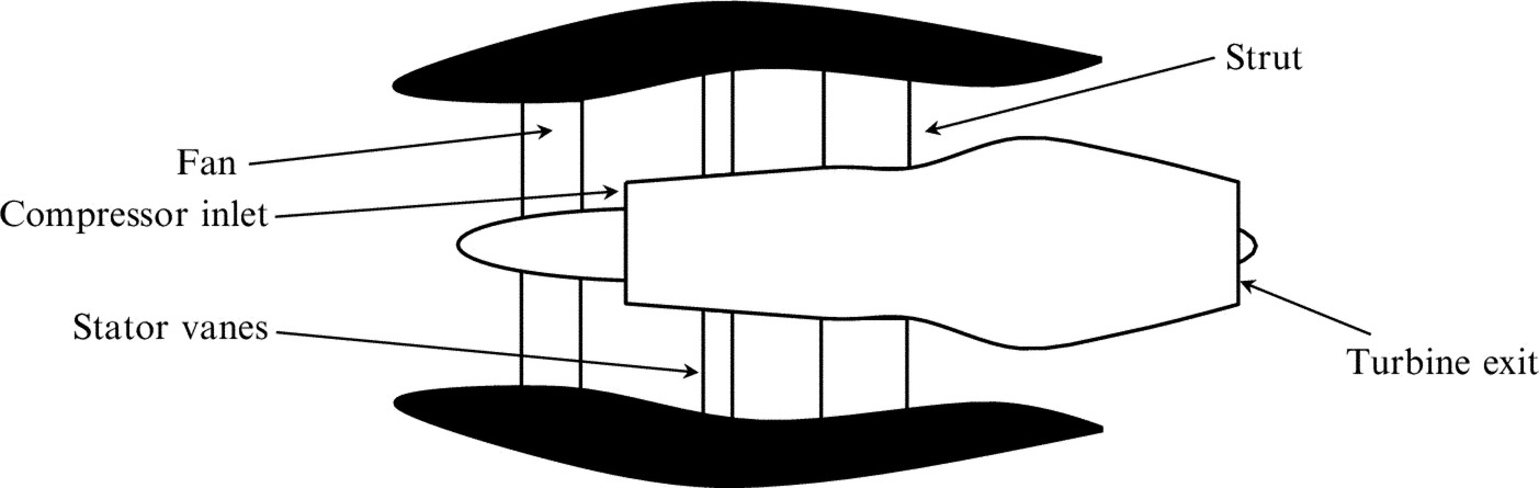
The design of a typical high bypass-ratio aircraft engine is shown in Fig. 17.1. The outer duct extends from the engine inlet to the bypass duct exit and is supported by the stator vanes and struts that are downstream of the fan. Just aft of the fan is the compressor inlet, which leads to the combustion chamber and the turbine, and the high speed flow generated by combustion exhausts through the turbine exit to form the jet core. The fan generates thrust, and the turbulent flow that results from the loaded fan blades impinges on the downstream stator vanes. The wake flow is highly turbulent and has a swirling motion, and the stator vanes are designed to reduce the swirl, recovering the energy lost to angular momentum downstream of the fan. The primary source of noise in the engine has been found to be the impingement of the wake from the fan onto the stator vanes.
In general, the outer duct of the engine is circular, but in some applications the inlet is modified so that it interferes less with the aerodynamic performance of the aircraft or enables additional ground clearance when the engine is mounted below the wing. The duct shape also has a varying cross section, and this can impact the propagation of acoustic waves along the duct. However, a great deal can be learned from studying the acoustic propagation in circular ducts and treating the variations in the duct cross section as a second-order effect. However, there are instances when the variation in duct cross section is vital to the understanding of sound propagation, and we will discuss these effects in more detail later.
In the analysis given in this chapter we will assume that sound propagation along the duct is linear, which implies the use of Goldstein's equation given in Chapter 6, and excludes the nonlinear propagation of sound associated with buzz-saw noise (noise caused by the rotating shock structure produced when the rotor is operated supersonically). We will limit consideration to circular ducts with a steady mean flow, which may be a function of radius and may include a swirling flow. We will also evaluate the effect of liners on the duct walls and radiation from the duct exits upstream or downstream of the fan. In general, we will consider these effects as idealized with simple boundary conditions so that we can identify the physical effects that are taking place. For an accurate calculation for aeroacoustic sources in a duct, numerical methods must be used. However, these are beyond the scope of the current treatment, and so references will be provided when appropriate.
17.2 The sound in a cylindrical duct
17.2.1 General formulation
We start by considering the linear acoustics problem of sound propagation in a cylindrical duct that has a mean flow. It will be assumed that the mean flow is uniform in the axial direction and that there are no vortical or turbulent perturbations introduced upstream of the region of interest. The duct will initially be taken to be infinitely long, but in later sections we will consider ducts of finite length.
Given these assumptions we can use Goldstein's equation to describe the acoustic waves in the duct in terms of the velocity potential ϕ as a function of the cylindrical coordinates (R,φ,x) shown in Fig. 17.2A. We will also consider cases when the duct has a center body as shown in Fig. 17.2B. Expressing Goldstein's equation (in the form of Eq. (6.3.2) with no source term) in cylindrical coordinates with an axisymmetric mean flow and a uniform sound speed and mean density, yields


We will solve this equation for a harmonic time dependence exp(−iωt) and a mean flow in the axial direction. We make use of the fact that the sound field is periodic in the azimuthal direction, so the potential can be expanded as a Fourier series giving
where ![]() are the complex Fourier series coefficients of order m that define the sound field. This simplifies Eq. (17.2.1) to
are the complex Fourier series coefficients of order m that define the sound field. This simplifies Eq. (17.2.1) to
where M=U/c∞ is the Mach number of the axial flow. Eq. (17.2.3) is the basic equation that describes the wave propagation in a circular duct.
17.2.2 Hard-walled ducts
The solution of this equation will depend on the boundary conditions that are imposed. We will start by requiring that the duct walls are hard and velocity perturbations in the direction normal to the wall are zero. If the mean flow is independent of the radius, then we can use the method of separation of variables to find a solution to Eq. (17.2.3). In this approach we specify
then Eq. (17.2.3) can be simplified by substituting for ![]() and dividing by Xmψm, so
and dividing by Xmψm, so

The second and third terms are independent of R and so must be equal to a constant if this equation is to apply for all values of x. We will choose this constant to be −κ2, and so we obtain

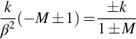
To solve the first of these two equations we can seek a solution in the form Xm(x)=Cmexp(iμx), where Cm is a constant. The value of μ is then obtained from the dispersion relationship, by substituting this expansion for Xm(x) into the first expression in Eq. (17.2.6)
which has two possible solutions given by

Similarly, we can solve the second of the two equations in Eq. (17.2.6) by multiplying through by ψm and expanding the differential, so

This is Bessel's equation which has the well-known solution
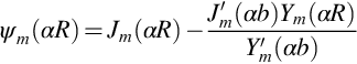
where Jm(αR) and Ym(αR) are Bessel functions of the first and second kind of order m and are illustrated in Fig. 17.3. We see that the Bessel function of the first kind is finite for all values of αR and is zero at αR=0 for all orders m≠0. In contrast the Bessel functions of the second kind are infinite at αR=0 for all orders. Both functions are oscillatory for large values of αR and decay to zero as (αR)−1/2 for large arguments.

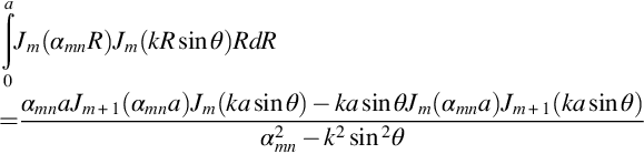
For the special case when the duct has no center body the sound field must remain finite at R=0, and this eliminates Ym(αR) as a possible solution. The sound field in the duct then only depends on Jm(αR). However, the solution must also match the non-penetration boundary condition on the outer duct wall, and so we require that the derivative of Jm(αR) with respect to R is zero at the wall where R=a. This is only possible for values of α for which ∂Jm(αR)/∂R=0 when R=a. There will be an infinite number of values of α that meet this condition, and they will be defined as αmn. For example, Fig. 17.4A and B shows the functions ψm(αmnR)=Jm(αmnR) for different values of m and n. Of particular note is the case when m=0, n=0 for which αmn=0. This represents the plane wave mode that has no radial variation, so the sound field is constant across the duct.

If the duct has a center body with radius b then the boundary condition at R=b is satisfied if the derivative of ψm(αR) with respect to R is zero at both walls. The boundary condition at R=b is met if
where the prime represents a differentiation with respect to the argument of the function. To satisfy the boundary condition on the outer wall α must take on the values for which

As with the duct without a center body there are an infinite number of solutions to this equation, and each represents a characteristic function or mode of propagation defined by the functions ψm(αmnR). Examples of these modes for a duct with a center body are shown in Fig. 17.4C and D. Note that the m=0, n=0 case yields a plane wave for which αmn=0 as was the case for the duct without a center body.
Eq. (17.2.8) is also identifiable as a Sturm Liouville equation with boundary conditions ![]() . The theory of differential equations shows that the solution of this equation is given by the sum of a set of eigenfunctions of the form
. The theory of differential equations shows that the solution of this equation is given by the sum of a set of eigenfunctions of the form

We commonly refer to the eigenfunctions as modes of propagation, and each mode individually satisfies the boundary conditions. Furthermore, Sturm Liouville theory shows that the modes are orthogonal which means that

where Cmn is a constant. Using the properties of the Fourier series that was used to expand the solution as a function of azimuthal angle φ (Eq. 17.2.2) we then find that

This is a valuable property that we will use to identify modes and evaluate how they are coupled to acoustic sources in the duct. Note that the integral is now over the duct cross-sectional area, and we can define the constant Λmn as
where S is the duct cross sectional area.
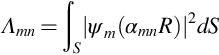
The key element required to define the modes is the wavenumbers αmn that are solutions to ![]() . For the duct without a center body for which ψm(αmna)=Jm(αmna) these values are tabulated and readily available. For large values of n there is also an asymptotic solution given by
. For the duct without a center body for which ψm(αmna)=Jm(αmna) these values are tabulated and readily available. For large values of n there is also an asymptotic solution given by
For a duct with a center body an approximate high-frequency solution can be obtained for the mode shapes given by Eq. (17.2.9) by using the large argument approximations of the Bessel functions
The approximate mode shapes of a hard-walled duct with a center body are then

where the normalization of the amplitude of the mode has been chosen for convenience (see below), and the wavenumbers are given by the solutions to tan(α(a−b))=1/2αa. For large arguments this gives, to a first approximation, αmn=nπ/(a−b). The important aspect of this result is that for ducts with center bodies the mode shapes are characterized by a relatively simple function that closely resembles a cosine wave with maxima or minima at the duct walls and n zero crossing points, as illustrated in Fig. 17.4C and D.
Finally, we note that the normalization parameter for a duct without a center body is given by

and for the duct modes with a center body Λmn=(a2−b2)π which is the cross-sectional area of the duct and justifies the choice of normalization used in Eq. (17.2.13).
17.2.3 Modal propagation
We can now summarize these results and combine Eqs. (17.2.2), (17.2.4) to give the modal description of sound propagation in a duct as

where from the dispersion relationship (17.2.7) and (17.2.8) we define
as the wavenumber that specifies the propagation in the axial direction. This is more conveniently written by rearranging terms as

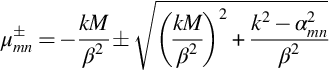
This wavenumber tells a great deal about the wave propagation in the duct. First we note that the ± sign is chosen to represent waves propagating in the positive or negative x direction when the value of the square root is real and taken to be positive. When the argument of the square root is negative (which occurs when βαmn>k) then it must have a positive imaginary part to ensure that the wave decays in the direction of propagation. It follows that waves will either propagate as waves or decay with distance in either the upstream or downstream direction as defined by the ± sign in Eq. (17.2.16). When the waves decay they are classified as being cutoff, and when they propagate they are defined as being cut on. The rate of decay depends on the “cutoff” ratio
If the cutoff ratio is large χmn≫1 then the value of ![]() has a large positive or negative imaginary part, and the duct mode of order m,n decays rapidly with distance along the duct. On the other hand, when the cutoff ratio is very small then the value of kmn is real, and the duct mode of order m,n propagates along the duct without attenuation with the wavenumber
has a large positive or negative imaginary part, and the duct mode of order m,n decays rapidly with distance along the duct. On the other hand, when the cutoff ratio is very small then the value of kmn is real, and the duct mode of order m,n propagates along the duct without attenuation with the wavenumber
which is consistent with upstream or downstream propagation of a plane wave in a uniform flow with Mach number M. When the cutoff ratio χmn is of order 1 then the modes are said to be close to cutoff and kmn tends to zero.
The decay of cutoff modes is an important feature of duct acoustics because it limits the number of acoustic modes that will propagate from a source to a duct exit, where they can radiate to the acoustic far field. If the source is a large distance from the duct exit then the cutoff modes play no role in the far-field radiation, but if the source is close to the duct exit then cutoff modes cannot be neglected. The rate of decay of a cutoff mode depends on
where |x| is the distance from the source. When χmn≫1 the amplitude of the mode decays to zero over a distance that is a fraction of an acoustic wavelength. However, when the mode is close to cut off then the decay is relatively slow. This is important because the fan design can be tailored so that the acoustic modes are cutoff, and this can result in significant far-field noise reductions.
An important property of Bessel functions is that the first zero of Jm′(αa) will occur when αa>m. Consequently, for a duct without a center body there will only be propagating duct modes when
and, as a consequence, modes will only propagate when 2πa/λ>βm. This is the ratio of the duct circumference to the acoustic wavelength and must be greater than m in order for the mode of order m to be cut on.
Another feature of the modal expansion of the sound field (Eq. 17.2.15) is that the modes are spinning as they propagate along the duct. The axial propagation speed is given by ![]() , and the speed of angular rotation is given by ω/m. Since ka/β>m it follows that the angular speed at the outer duct wall is ωa/m>ωβ/k=c∞β. The angular speed of a propagating mode at the duct wall is therefore supersonic. This is an important characteristic of duct propagation because it implies that rotating sources, such as fans with subsonic tip speeds, will not couple directly with propagating acoustic modes. This issue will be discussed in more depth in the next chapter where it will be shown that subsonic fan noise sources only couple with duct modes if their rate of rotation is “stepped up” or increased by source interactions that effectively increase their rate of rotation.
, and the speed of angular rotation is given by ω/m. Since ka/β>m it follows that the angular speed at the outer duct wall is ωa/m>ωβ/k=c∞β. The angular speed of a propagating mode at the duct wall is therefore supersonic. This is an important characteristic of duct propagation because it implies that rotating sources, such as fans with subsonic tip speeds, will not couple directly with propagating acoustic modes. This issue will be discussed in more depth in the next chapter where it will be shown that subsonic fan noise sources only couple with duct modes if their rate of rotation is “stepped up” or increased by source interactions that effectively increase their rate of rotation.
17.3 Duct liners
In the previous section it was assumed that the duct had a hard wall so that the acoustic perturbation velocity normal to the wall was zero. In a lined duct the relationship is more complicated and defined by the liner impedance which is a complex quantity given by the ratio of the pressure imposed on the liner to the acoustic velocity normal to the surface ![]() where both the pressure and particle velocity have a harmonic time dependence exp(−iωt). The wall is assumed to be locally reacting, which implies that acoustic waves do not propagate within the liner. To match the motion of the fluid with the motion at the liner we must ensure that the displacement normal to the surface ξ is equal to the fluid particle displacement at the same point. The particle velocity of the fluid normal to the surface is given by the rate of change of the particle displacement in a frame of reference moving with the mean flow, so the relationship between the acoustic velocity potential ϕ and the acoustic particle displacement is
where both the pressure and particle velocity have a harmonic time dependence exp(−iωt). The wall is assumed to be locally reacting, which implies that acoustic waves do not propagate within the liner. To match the motion of the fluid with the motion at the liner we must ensure that the displacement normal to the surface ξ is equal to the fluid particle displacement at the same point. The particle velocity of the fluid normal to the surface is given by the rate of change of the particle displacement in a frame of reference moving with the mean flow, so the relationship between the acoustic velocity potential ϕ and the acoustic particle displacement is

where n is the unit normal to the surface. To obtain a boundary condition for the acoustic velocity potential with a harmonic time dependence we use the relationship between the pressure and the potential given by Eq. (6.1.7) so that

For the liner, however, the relationship between its displacement and velocity normal to the surface is vs=∂ξ/∂t, and so
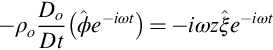
We take the substantial derivative of Eq. (17.3.2) and linearize Eq. (17.3.1) about the mean flow to obtain the boundary condition

The boundary conditions for the Sturm Liouville problem discussed in the previous section need to be modified to account for the liner. Using Eq. (17.3.3) we find that boundary condition for the radial modes in Eq. (17.2.15) becomes
where the wavenumber of propagation along the duct is defined as a function of the radial wavenumber as given by Eq. (17.2.16). This is often written in terms of the nondimensional admittance βa=ρoc∞/z and takes the form
This is a far more complicated boundary condition than for a hard-walled duct (which has an admittance of zero) and needs to be computed numerically. However, some insight can be obtained by considering approximate solutions for small admittances and no axial flow. Considering a Taylor series expansion of Eq. (17.3.5) gives
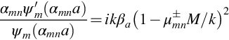
where αmn(o)a are the solutions for the hard-walled duct, and so ![]() . From Eq. (17.2.8) we find that
. From Eq. (17.2.8) we find that

and so we can approximate Eq. (17.3.5) when M=0 as
This gives a relatively simple approximation for the radial wavenumber.
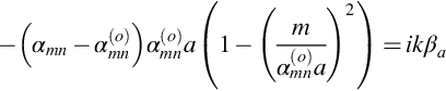
To determine the effect on mode attenuation along the duct we need to consider the axial wavenumber, which, for zero flow, can be approximated from Eq. (17.2.16) as

and combining this with Eq. (17.3.6) we obtain

This shows that the effect of the liner impedance is to give the axial wavenumber an imaginary part, which causes the modes to attenuate as they propagate along the duct. The amount of attenuation is determined by not only the admittance but also the wavenumbers of propagation. For the lowest order mode, we have noted in Section 17.2 that m/αmo(o)a is approximately 1, and so this mode will be highly attenuated by the liner because the imaginary part of the axial wavenumber will be large. However, this effect is reduced for the higher-order radial modes for which ![]() . Similarly, close to the cutoff frequency kmn(o) will be small, and so the effect of the liner will be large. It follows that liners are important at reducing levels close to cutoff where typically duct mode power levels are high.
. Similarly, close to the cutoff frequency kmn(o) will be small, and so the effect of the liner will be large. It follows that liners are important at reducing levels close to cutoff where typically duct mode power levels are high.
The more general result, with flow, requires a solution to Eqs. (17.3.5), (17.2.16), and can be achieved by evaluating these functions for different values of αmn/k (both real and imaginary) and determining βa and ![]() . For example, in Fig. 17.5 we show contours of the admittance |βa|, and its phase plotted against the real and imaginary parts of
. For example, in Fig. 17.5 we show contours of the admittance |βa|, and its phase plotted against the real and imaginary parts of ![]() . In this case the flow Mach number is 0.3 and ka=2, and there is no center body in the duct. Note that for a hard wall the admittance is zero, and the curves lie on the real axis at
. In this case the flow Mach number is 0.3 and ka=2, and there is no center body in the duct. Note that for a hard wall the admittance is zero, and the curves lie on the real axis at ![]() , which is the phase speed for the m=1 mode propagating upstream at this frequency. As the magnitude of the admittance is increased the imaginary part of
, which is the phase speed for the m=1 mode propagating upstream at this frequency. As the magnitude of the admittance is increased the imaginary part of ![]() is no longer zero and takes on significant negative values, which attenuates the mode as it propagates. For the wave to decay as it propagates upstream the imaginary part of
is no longer zero and takes on significant negative values, which attenuates the mode as it propagates. For the wave to decay as it propagates upstream the imaginary part of ![]() must be negative as shown, and the attenuation of this mode in decibels is given by
must be negative as shown, and the attenuation of this mode in decibels is given by ![]() and gives an attenuation of about 10 dB per wavelength when the magnitude of the admittance is >0.2 and the phase lies in the range ±30 degrees.
and gives an attenuation of about 10 dB per wavelength when the magnitude of the admittance is >0.2 and the phase lies in the range ±30 degrees.

17.4 The Green's function for a source in a cylindrical duct
To analyze aeroacoustic sources in a duct we can make use of either Curle's theorem or the Ffowcs-Williams and Hawkings equation written in terms of a suitable Green's function. In general, a Green's function in a duct with a nonuniform mean flow and liners is not readily available in an analytical form, but we can obtain useful results by limiting consideration to a uniform flow in a hard-walled duct. The more complex situation of sources in a nonuniform swirling flow will be considered in Section 17.6. For the case of uniform flow in a hard-walled duct the Green's function is chosen so that its derivative normal to the duct wall is zero. The surface integrals over the duct walls in the Ffowcs-Williams and Hawkings equation (5.2.9) are thus eliminated, and only the surface integrals over the fan blades and stator vanes need to be considered. It should also be noted that Lighthill's equation only applies in a uniform mean flow. If the flow in the duct is nonuniform, then this has to be accounted for separately in the evaluation of the source terms. In principle this can be achieved by coupling the wave field in the duct to the source terms on a Ffowcs-Williams and Hawkings surface surrounding the sources in the acoustic near field and using a separate solution for the wave propagation in the duct. However, the key part of the calculation remains as the evaluation of the Ffowcs-Williams and Hawkings equation using a Green's function with a uniform mean flow, that is the solution to

As in Section 3.10 we will first consider the Green's function defined in terms of its Fourier transform with respect to time. We can then use Eq. (3.10.7) to obtain the equivalent result in the time domain, which can be used in Eq. (5.4.4) for a source in a duct with flow. Substituting Eq. (3.10.7) into the equation above and evaluating all the integrals gives the Green's function in the frequency domain as the solution to

where the right-hand side of this equation is defined in cylindrical coordinates and meets the requirements of Eq. (3.9.4). The source location is given by (Ro,φo,xo) and the observer location by (R,φ,x), and the flow is defined as being uniform in the axial direction with speed U so that M=U/c∞. Note also that the sign of the exponent in the definitions in Eq. (3.10.7) determines the signs of the terms on the left of this equation because the differential is carried out with respect to τ.
In the region x<xo or x>xo this equation is identical to the homogeneous equation for sound propagation in a duct with flow −U in the axial direction (see Eq. 17.2.3), so we expect the solution to have the same form as Eq. (17.2.15), and we can expand the Greens function as a set of modes given by

where the sign in the exponent is chosen as positive when xo>x and as negative when xo<x (as will be justified below). As it stands this solution is discontinuous at x=xo and if it is used in Eq. (17.4.1) we will have to account for the discontinuity in the evaluation of the derivatives with respect to xo. If the mode amplitudes are continuous at the source point, then it follows that

When this result is used in Eq. (17.4.1) and the derivatives are evaluated using

we find that the differential equation for the Green's function reduces to

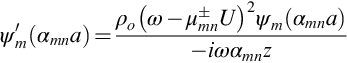
Since the modes form an orthogonal set we can use Eq. (17.2.10) to extract the mode amplitudes from this equation by multiplying each side by ψm(αmnR)eimφ and integrating over the duct cross section, giving

and so the Green's function is given by
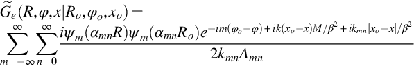
and the solution in the time domain is obtained from the inverse transform specified in Eq. (3.10.7).
This result is fundamental to the understanding of sound propagation in a duct because it shows how sound will propagate from a source at (Ro,φo,xo) to an observer at (R,φ,x). When x>xo then the waves propagate downstream with the same phase dependence as given by the modal expansion (17.2.15) and (17.2.16). Similarly, when x<xo the waves are propagating upstream with the correct phase dependence. We also note that this result is not reciprocal. If the source and observer positions are interchanged then the phase factor that depends on ik(xo−x)M/β2 will be reversed, and so the wave fields are not identical unless M=0. Reciprocity is only achieved if the direction of the flow is also reversed, and this is known as the reverse flow theorem, which applies for all sources in a steady flow not only when they are in a duct.
The Green's function represents the sound from a point monopole or volume displacement source, and Eq. (17.4.2) shows how this depends on the radial location of the source. If the source is located at a null of the radial mode shape, then it does not couple with the acoustic field in the duct and that mode is not excited. In contrast if the source is located at a maximum of the radial mode shape then that mode is strongly excited, and if that mode is close to cutoff (![]() ) then it could dominate the sound field in the duct. Similar results apply to dipole and quadrupole sources since their acoustic efficiency is given by the derivative of the Green's function along the axis of the dipole. This can impact the efficiency of each mode because the derivatives will introduce a factor that depends on the mode wavenumber and/or order. This will be discussed in more detail in Chapter 18.
) then it could dominate the sound field in the duct. Similar results apply to dipole and quadrupole sources since their acoustic efficiency is given by the derivative of the Green's function along the axis of the dipole. This can impact the efficiency of each mode because the derivatives will introduce a factor that depends on the mode wavenumber and/or order. This will be discussed in more detail in Chapter 18.
17.5 Sound power in ducts
In Section 2.6 we introduced the concept of sound power. An important application of this concept is to duct acoustics. Since waves propagate along the duct and out of the duct exit to the far field via a complicated path (see Fig. 17.1) the concept that sound power is conserved allows us to relate the in duct sound levels directly to the far field, assuming that there is no absorption at the duct walls and no sound power is reflected back toward the source by the duct exits or internal features. This of course is an important assumption that only applies for ducts of large diameter compared to the acoustic wavelength. For small diameter ducts such as car exhausts, the acoustic wavelength is large compared to the duct diameter and the reflections at the exhaust exit and at changes of cross section, such as the muffler, completely control the sound power radiated to the far field. In contrast on an aero engine the duct diameter is so large that waves propagate freely out of the inlet or exhaust, and reflections back toward the source are of secondary importance. This characteristic is very important for engine design purposes because it means that the sound power provides a measure of the effective noise source level, which corresponds to the expected level of the far-field sound.
In Section 2.6 we defined the sound power from a source in a volume bounded by the surface S as

where I is the acoustic intensity vector and n is the unit normal vector pointing out of the volume containing the sources. In a hard-walled duct, the intensity is zero normal to the duct walls, and so the integral is carried out over the duct cross sections upstream or downstream of the source. We can therefore split the sound power into its upstream and downstream components, which radiate from the engine inlet or exit, respectively.
The acoustic intensity in a moving fluid is given by Eq. (2.6.17) in terms of the acoustic particle velocity and acoustic pressure perturbations as
In the absence of vortical waves ![]() and the pressure perturbation is given by
and the pressure perturbation is given by ![]() , so
, so
The intensity can then be written in terms of the velocity potential as

For waves with harmonic time dependence we can reduce this result using the approach given in Section 3.8 so that
For upstream or downstream propagating waves we need to consider the component of the intensity in the positive or negative axial direction and integrate over the cross section of the duct. For a uniform flow we can define the acoustic velocity potential using the modal expansion given by Eq. (17.2.15) so that
where the normal vector points away from the source and the ± refers to downstream or upstream propagation, respectively. The terms in the curly braces simplify to give ![]() . When these results are used in Eq. (17.5.2) and the surface integral is carried out over the duct cross section, then we can make use of the orthogonality of the duct modes, given by Eq. (17.2.10), to obtain the sound power in either the upstream or downstream directions as
. When these results are used in Eq. (17.5.2) and the surface integral is carried out over the duct cross section, then we can make use of the orthogonality of the duct modes, given by Eq. (17.2.10), to obtain the sound power in either the upstream or downstream directions as
This remarkably simple result has some important implications. First we note that the power for each mode is uncoupled, so we can treat a noise control problem mode by mode. Furthermore, the level is not simply a function of the mode amplitude but is also determined by the normalization factor Λmn and the real part of the wavenumber kmn. If the mode is cutoff, then kmn is imaginary, and there is no sound power transmitted in that mode. Consequently, only propagating modes contribute to the far-field sound power levels. An important result is that for a source in a duct the duct mode amplitudes are given by the Green's function specified in Eq. (17.4.2). This shows that the duct mode amplitudes are inversely proportional to kmnΛmn, and so the sound power will tend to infinity at the cut on frequency where kmn is zero unless the source strength also tends to zero. This issue will be discussed in more detail in Chapter 18.
The consequence of this result is that if we use the modal sound power to evaluate sources in the duct only the amplitude of propagating modes needs be considered. Since these are limited to a finite number of modes the infinite summations in Eq. (17.5.3) are no longer required making their evaluation tractable.
17.6 Nonuniform mean flow
In Section 17.3 a formulation was given for acoustic propagation in a cylindrical duct with a uniform mean flow. It was shown that a modal solution could be obtained by using the method of separation of variables, so the wave equation was reduced to solving a Sturm Liouville equation. However, when the mean flow is not uniform the wave equation is not separable, and we must resort to other methods to find a solution. The most general approach is to use a numerical method to solve the appropriate differential equation with the correct boundary conditions as described by Astley and Eversman [1,2] and Golubev and Atassi [3]. However, some insight to the problem is obtained if a high-frequency approximation is used to obtain the solution to the wave equation in a hard-walled duct with nonuniform flow (Cooper and Peake [4]).
To show how the high-frequency approximation can be applied, it is assumed that the mean flow is only a function of the radial coordinate and is given by the sum of an axial component U(R) and an azimuthal component W(R)=Ω(R)R. We will assume no mean radial flow, which is an important simplification and ignores the interaction of the mean flow with the turbulent wakes of the fan blades. It will also be assumed that there are no vortical waves in the duct, so the acoustic field is completely described by the velocity potential that satisfies the convected wave equation given in Eq. (17.2.1). We can assume that the velocity potential has a harmonic time dependence and make use of the periodicity in the azimuthal direction to expand the potential in a Fourier series as given by Eq. (17.2.2). The resulting Fourier series coefficients satisfy the differential equation given by

where
is the effective acoustic wavenumber in a swirling flow and will be a function of radius unless the mean flow is in solid-body rotation. The difference between Eq. (17.6.1) and Eq. (17.2.3) is that it is not separable because the coefficients are dependent on the radius. However, we can find a solution using the Wentzel–Kramers–Brillouin (WKB) method which gives an approximate solution in the high-frequency limit that ka≫1. To implement this approximation, we specify the potential as an exponential or phase function so that
where μ and Bm are constants and qm(R/a) is to be determined from the solution to Eq. (17.6.1). The mode shape is then given by exp(iqm(R/a)), and Eq. (17.6.1) becomes
where the prime represents differentiation with respect to the argument of qm and
For the analysis of the sound field in the duct with uniform flow we expect μ/k and m/ka to be of order one, and so it follows that λm is of order O(ka), which is a large parameter in the high-frequency limit ka≫1. We consider a solution that is of the form
where both qm(o) and qm(1) are the same order of magnitude. In terms of these variables Eq. (17.6.4) becomes

each term in this equation is therefore defined in descending orders of ka. The principle of the WKB method is that when ka≫1 the first term is large compared to the second two terms, and so an approximate solution is obtained for qm(1) as

To obtain a solution that is accurate to second order the second term in Eq. (17.6.6) can also be set to zero, giving
We have therefore reduced the problem to solving two first-order differential equations that have the solutions
(where b is the radius of the inner duct wall, and we have used the fact that ![]() ). The approximate solution to the wave equation in the high-frequency limit is then given by
). The approximate solution to the wave equation in the high-frequency limit is then given by
This gives two alternative solutions for the acoustic field in a duct with a mean flow that is a function of radius, and the two solutions can be combined to match the boundary conditions at the duct walls. The radial dependence of the modes depends on the integral defining qm(1) in Eq. (17.6.7) which takes the form
The first point to note from this result is that at small radii the term (m/R)2 may be large enough that the integrand is imaginary, but as R increases a branch point is reached where the integrand is zero and at larger radii it becomes real valued. This causes the integrand to have a critical point defined by the value of R=Rc where the integrand is zero.
To match the boundary conditions, we specify

where the square roots are evaluated so that their real parts are positive. Using this form of the solution the hard-walled boundary condition is met on the inner duct wall to first order in 1/ka, and to the same order we must solve for μ in Eq. (17.6.5) so that kaq(1)(a)=nπ to match the boundary condition on the outer wall, which can be done iteratively if λm2(R)>0 for b<R<a.
However, this solution does not apply close to the so-called critical radius where λm is approximately zero, and so the high-frequency approximation is no longer strictly valid. A solution can be obtained by solving Eq. (17.6.1) in the vicinity of the critical point and the result is given by Cooper and Peake [4] in terms of Airy functions. This needs to be matched to the solution valid outside the critical region defined by Eq. (17.6.9). In the region where λm2 is negative the mode shapes are given by a hyperbolic cosine, which needs to be matched to the solution in the critical region. The net effect is that the mode amplitude tends to zero when λm2(R)<0.
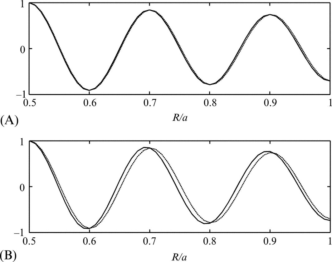
In the absence of swirl and for a uniform axial flow the approximate solution reduces to the form of the Bessel function solutions given in the previous section in Eq. (17.2.12) and shown in Fig. 17.4. The accuracy of the approximation is shown in Fig. 17.6A for m=2 and ka=50 for no axial flow. The advantage of the high-frequency analysis is that it allows the mean axial flow and swirl to be a function of radius. To illustrate this Fig. 17.6B shows the mode shape when the mean flow speed varies with radius as M(R)=MtR/a in comparison with the zero flow case.
The effect of solid-body swirl, in which Ω is constant, is to alter the effective frequency, so depending on the sign of m, the cut on frequency is shifted from ωo without swirl to the effective frequency |ωo±mΩ|, and this can have important implications for the number of modes that propagate.
It was also pointed out by Cooper and Peake [4] that some interesting possibilities occur when λm(R) has more than one zero in the range b<R<a. In this case there is the possibility for two or more critical radii, and so the sound field can be trapped between these points, giving rise to loud zones and quiet zones radially in the duct. These zones exist if both λm2(a) and λm2(b) are less than zero and that λm2(R) is greater than zero at some location across the duct. If the swirl velocity is of the form Ω(R)=Ωo+Γ/R2, corresponding to the combination of solid-body rotation and a potential vortex, then ω+mΩ(R) will be less at the outer wall than at the inner wall, and a mode that is cut on at a small radius could be cut off at the larger radius because the effective frequency is less.
17.7 The radiation from duct inlets and exits
So far in this chapter we have discussed the propagation of acoustic modes in circular ducts of infinite length. In a turbofan engine (Fig. 17.1) the duct will vary in cross section and will be of finite length, and it is the radiation out of the duct inlets and exits that is of primary concern. There are a number of numerical approaches that can be used to address a real duct, including Finite Element Methods [1,2] and the Geometrical Theory of Diffraction [5,6]. Small variations in the cross section of the duct can also be considered using multiple scale analysis [7]. We can also gain insight into radiation from a duct inlet or exit using analytical methods, and these are discussed in this section.
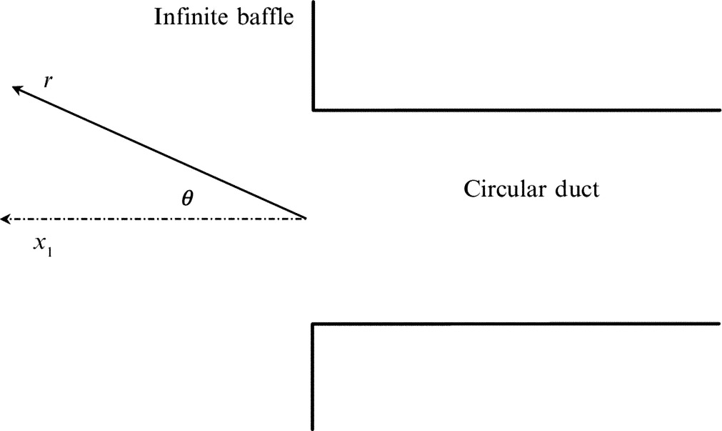
Analytical models of the sound radiation from a duct are most readily obtained by considering a semi-infinite circular duct as illustrated in Fig. 17.7. In the case of the duct exit or jet pipe (Fig. 17.7A) the flow inside the duct is taken to be uniform and the flow speed outside the duct can be different so that a shear layer is formed between the two flows, and this can cause shear layer refraction effects and the possibility of instability waves at the interface. In the case of an inlet (Fig. 17.7B) the flow is taken to be uniform both inside and outside the duct.

The sound radiation from semi-infinite pipes with flow is described by Munt [8], who analyzed the problem using the Weiner Hopf method. However, Tyler and Sofrin [9] argued that a good approximation to the far-field sound from an inlet without flow is obtained by modeling the inlet by a circular duct that is mounted in a baffle, as shown in Fig. 17.8. Lansing [10] studied the equivalence between these two approximations and showed that there were only small differences in the radiated sound power between the two cases. The differences occurred at frequencies close to cutoff, as might be expected. However, the Tyler and Sofrin model cannot give the correct directivity at angles >90 degrees to the duct axis because this observer would be inside the baffle.
An alternative approximation was given by Cargill [11] who used a Ffowcs-Williams and Hawkings surface on the external surface of a semi-infinite pipe, and the pipe exit, for the configuration shown in Fig. 17.7A. A Green's function was developed for a source in the jet pipe flow with different flow speeds on either side of the shear layer. A key assumption was that the contribution from the external surface of the pipe was negligible compared to radiation from the duct exit. In spite of this apparently major simplification it was shown that the far-field sound was almost identical to Munt's exact solution at all but a few observer angles in the region upstream of the jet pipe exit.
To illustrate Cargill's method, we will consider the sound radiation from an inlet without flow, using the coordinates given in Fig. 17.7A, with U=0. The solution for the acoustic field outside the duct is given by Eq. (3.10.5) with the surface taken as the external surface of the duct and the duct exit. In Cargill's approximation only the duct exit is included, and the acoustic pressure and its normal derivative are defined by the waves propagating along the duct toward the duct exit. This implies that no waves are reflected back toward the source inside the duct, which is a reasonable approximation when ka≫1. The far-field sound is then given by Eq. (3.10.5) for a harmonic time dependence
If we limit consideration to a single duct mode and integrate over the duct exit, we obtain the pressure as
where Bmn is the pressure amplitude of the duct mode. For a duct without a center body ψm(αmnR)=Jm(αmnR). The free field Green's function can be approximated for observers in the acoustic far field of the duct by

where r is the distance from the center of the duct exit to the observer located at x1=rcosθ, x2=rsinθ, x3=0 as shown in Fig. 17.7A. Using y1=0, y2=Rcosφ, y3=Rsinφ, the acoustic far field is given by

The integral over the azimuth gives
and the integral over the radius is a standard integral given by
For a hard-walled duct ![]() , and we can use the Bessel function recurrence relationships to simplify this result to
, and we can use the Bessel function recurrence relationships to simplify this result to

The far-field sound is then given by

where the directivity is

Fig. 17.9 shows the directivity of the far-field sound based on Eq. (17.7.2) and is compared to computations based on the full Weiner Hopf solution [12]. It is seen that the approximate solution is very accurate at angles where the directionality is a maximum but fails to give the correct result at large angles where the levels are about 10 dB less than the peak values. This is consistent with Cargill's [11] observation that the error was in the region of the far field where that particular mode did not significantly contribute to the overall level.
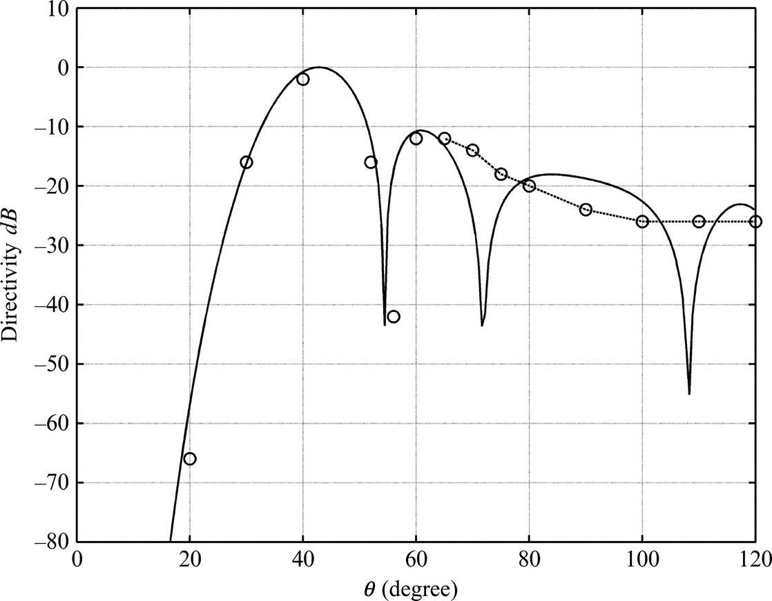
It is clear from Fig. 17.9 that the far-field sound peaks at an angle to the duct axis where ksinθ=αmn where the denominator of Eq. (17.7.2) is zero. At this angle the directivity can be evaluated using L'Hôpital's rule because Jm′(ka sin θ) is also zero when ksinθ=αmn. The directivity therefore has similar characteristics to a sin(x)/x function with a peak at the location where x=0, and side lobes of a lower level on either side of the peak.