Chapter 10: Profitability Analysis

This chapter will explain how to apply the techniques of economic analysis developed in Chapter 9. These techniques will be used to assess the profitability of projects involving both capital expenditures and yearly operating costs. A variety of projects will be examined, ranging from large multimillion-dollar ventures to much smaller process improvement projects. Several criteria for profitability will be discussed and applied to the evaluation of process and equipment alternatives. The first concept is the profitability criteria for new large projects.

10.1 A Typical Cash Flow Diagram for a New Project

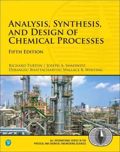
A typical cumulative, after-tax cash-flow diagram (CFD) for a new project is illustrated in Figure 10.1. It is convenient to relate profitability criteria to the cumulative CFD rather than the discrete CFD. The timing of the different cash flows is explained below.

Figure 10.1 A Typical Cumulative Cash Flow Diagram for the Evaluation of a New Project

In the economic analysis of the project, it is assumed that any new land purchases required are done at the start of the project, that is, at time zero. After the decision has been made to build a new chemical plant or expand an existing facility, the construction phase of the project starts. Depending on the size and scope of the project, this construction may take anywhere from six months to three years to complete. In the example shown in Figure 10.1, a typical value of two years for the time from project initiation to the start-up of the plant has been assumed. Over the two-year construction phase, there is a major capital outlay. This represents the fixed capital expenditures for purchasing and installing the equipment and auxiliary facilities required to run the plant (see Chapter 7). The distribution of this fixed capital investment is usually slightly larger toward the beginning of construction, and this is reflected in Figure 10.1. At the end of the second year, construction is finished and the plant is started. At this point, the additional expenditure for working capital required to float the first few months of operations is shown. This is a one-time expense at the start-up of the plant and will be recovered at the end of the project.

After start-up, the process begins to generate finished products for sale, and the yearly cash flows become positive. This is reflected in the positive slope of the cumulative CFD in Figure 10.1. Usually the revenue for the first year after start-up is less than in subsequent years due to “teething” problems in the plant; this is also reflected in Figure 10.1. The cash flows for the early years of operation are larger than those for later years due to the effect of the depreciation allowance discussed in Chapter 9. The time used for depreciation in Figure 10.1 is six years. The time over which the depreciation is allowed depends on the IRS regulations and the method of depreciation used.

In order to evaluate the profitability of a project, a life for the process must be assumed. This is not usually the working life of the equipment, nor is it the time over which depreciation is allowed. It is a specific length of time over which the profitability of different projects is to be compared. Lives of 10, 12, and 15 years are commonly used for this purpose. It is necessary to standardize the project life when comparing different projects. This is because profitability is directly related to project life, and comparing projects using different lives biases the results.

Usually, chemical processes have anticipated operating lives much greater than ten years. If much of the equipment in a specific process is not expected to last for a ten-year period, then the operating costs for that project should be adjusted. These operating costs should reflect a much higher maintenance cost to include the periodic replacement of equipment necessary for the process to operate the full ten years. A project life of ten years will be used for the examples in the next section.

From Figure 10.1, a steadily rising cumulative cash flow is observed over the ten operating years of the process, that is, years 2 through 12. At the end of the ten years of operation, that is, at the end of year 12, it is assumed that the plant is closed down and that all the equipment is sold for its salvage or scrap value, that the land is also sold, and that the working capital is recovered. This additional cash flow, received on closing down the plant, is shown by the upward-pointing vertical line in year 12. It must be remembered that in reality, the plant will most likely not be closed down; it is only assumed that it will be to perform the economic analysis.

The question that must now be addressed is how to evaluate the profitability of a new project. Looking at Figure 10.1, it can be seen that at the end of the project the cumulative CFD is positive. Does this mean that the project will be profitable? The answer to this question depends on whether the value of the income earned during the time the plant operated is smaller or greater than the investment made at the beginning of the project. Therefore, the time value of money must be considered when evaluating profitability. The following sections examine different ways to evaluate project profitability.

10.2 Profitability Criteria for Project Evaluation

There are three bases used for the evaluation of profitability:

1. Time

2. Cash

3. Interest rate

For each of these bases, discounted or nondiscounted techniques may be considered. The nondiscounted techniques do not take into account the time value of money and are not recommended for evaluating new, large projects. Traditionally, however, such methods have been and are still used to evaluate smaller projects, such as process improvement schemes. Examples of both types of methods are presented for all three bases.

10.2.1 Nondiscounted Profitability Criteria

Four nondiscounted profitability criteria and the graphical interpretation of these profitability criteria are illustrated in Figure 10.2. Each of the four criteria is explained below.

Figure 10.2 Illustration of Nondiscounted Profitability Criteria

Time Criterion. The term used for this criterion is the payback period (PBP), also known by a variety of other names, such as payout period, payoff period, and cash recovery period. The payback period is defined as follows:

PBP = Time required, after start-up, to recover the fixed capital investment, FCI_L, for the project

The payback period is shown as a length of time on Figure 10.2. Clearly, the shorter the payback period, the more profitable the project.

Cash Criterion. The criterion used here is the cumulative cash position (CCP), which is simply the worth of the project at the end of its life. For criteria using cash or monetary value, it is difficult to compare projects with dissimilar fixed capital investments, and sometimes it is more useful to use the cumulative cash ratio (CCR), which is defined as

The definition effectively gives the cumulative cash position normalized by the initial investment. Projects with cumulative cash ratios greater than one are potentially profitable, whereas those with ratios less than unity cannot be profitable.

Interest Rate Criterion. The criterion used here is called the rate of return on investment (ROROI) and represents the nondiscounted rate at which money is made from a fixed capital investment. The definition is given as

The annual net profit in this definition is an average over the life of the plant after start-up.

The use of fixed capital investment, FCI_L, in the calculations for payback period and rate of return on investment given above seems reasonable, because this is the capital that must be recovered by project revenue. Many alternative definitions for these terms can be found, and sometimes the total capital investment (FCI_L + WC + Land) is used instead of fixed capital investment. When the plant has a salvage value (S), the fixed capital investment minus the salvage value (FCI_L – S) could be used instead of FCI_L. However, because the salvage value is usually very small, it is preferable to use FCI_L alone. Example 10.1 is a comprehensive profitability analysis calculation using nondiscounted criteria.

Example 10.1

A new chemical plant is going to be built and will require the following capital investments (all figures are in $million):

Cost of land, L = $10.0

Total fixed capital investment, FCI_L = $150.0

Fixed capital investment during year 1 = $90.0

Fixed capital investment during year 2 = $60.0

Plant start-up at end of year 2

Working capital = $30.0 at end of year 2

The sales revenues and costs of manufacturing are given below:

Yearly sales revenue (after start-up), R = $75.0/y

Cost of manufacturing excluding depreciation allowance (after start-up), COM_d = $30.0/y

Taxation rate, t = 45%

Salvage value of plant, S = $10.0

Depreciation: Use 5-year MACRS.

Assume a project life of 10 years.

Calculate each nondiscounted profitability criterion given in this section for this plant.

Solution

The discrete and cumulative nondiscounted cash flows for each year are given in Table E10.1. Using these data, the cumulative cash flow diagram is drawn, as shown in Figure E10.1.

Table E10.1 Nondiscounted After-Tax Cash Flows for Example 10.1 (All Numbers in $10⁶)

End of Year (k)	Investment	dk	FCIL — Σdk	R	COMd	(R-COM-dk) × (1—t) + dk	Cash Flow	Cumulative Cash Flow
0	(10)*	—	150.00	—	—	—	(10.00)	(10.00)
1	(90)	—	150.00	—	—	—	(90.00)	(100.00)
2	(60 + 30) = (90)	—	150.00	—	—	—	(90.00)	(190.00)
3	—	30.00	120.00	75	30	38.25	38.25	(151.75)
4	—	48.00	72.00	75	30	46.35	46.35	(105.40)
5	—	28.80	43.20	75	30	37.71	37.71	(67.69)
6	—	17.28	25.92	75	30	32.53	32.53	(35.16)
7	—	17.28	8.64	75	30	32.53	32.53	(2.64)
8	—	8.64	0.00	75	30	28.64	28.64	26.00
9	—	—	0.00	75	30	24.75	24.75	50.75
10	—	—	0.00	75	30	24.75	24.75	75.50
11	—	—	0.00	75	30	24.75	24.75	100.25
12	10 + 30 = 40	—	0.00	85	30	30.25	70.25	170.50
*Numbers in () are negative cash flows. Nondiscounted Profitability Criteria Payback Period (PBP) Land + Working Capital = 10 + 30 = $40 ×106—find time after start-up for which cumulative cash flow = −$40 ×106 PBP = 3 + (−67.69 + 40)/(−67.69 + 35.16) = 3.85 years Cumulative Cash Position (CCP) and Cumulative Cash Ratio (CCR) CCP = $170.50 × 106 and CCR = Σ positive cash flows/Σ negative cash flows = (38.25 + 46.35 + 37.71 + ... + 24.75 + 70.25) / (10 + 90 + 90) = 1.897 Rate of Return on Investment (ROROI) ROROI = (38.25 + 46.35 + 37.71 + ... + 24.75 + 30.25)/10/150 – 1/10 = 0.114 or 11.4% p.a.

Figure E10.1 Cumulative Cash Flow Diagram for Nondiscounted After-Tax Cash Flows for Example 10.1

The method of evaluation for each of the criteria is given in Figure E10.1 and Table E10.1.

Payback Period (PBP) = 3.85 years

Cumulative Cash Position (CCP) = $170.5 × 10⁶

Cumulative Cash Ratio (CCR) = 1.897

Rate of Return on Investment (ROROI) = 11.4%

All of these criteria indicate that the project cannot be eliminated as unprofitable. They all fail to take into account the time value of money that is necessary for a thorough measure of profitability. The effects of the time value of money on profitability are considered in the next section.

10.2.2 Discounted Profitability Criteria

The main difference between the nondiscounted and discounted criteria is that for the latter each of the yearly cash flows is discounted back to time zero. The resulting discounted cumulative cash flow diagram is then used to evaluate profitability. The three different types of criteria are:

Time Criterion. The discounted payback period (DPBP) is defined in a manner similar to the nondiscounted version given above.

DPBP = Time required, after start-up, to recover the fixed capital investment, FCI_L, required for the project, with all cash flows discounted back to time zero

The project with the shortest discounted payback period is the most desirable.

Cash Criterion. The discounted cumulative cash position, more commonly known as the net present value (NPV) or net present worth (NPW) of the project, is defined as

NPV = Cumulative discounted cash position at the end of the project

Again, the NPV of a project is greatly influenced by the level of fixed capital investment, and a better criterion for comparison of projects with different investment levels may be the present value ratio (PVR):

A present value ratio of unity for a project represents a break-even situation. Values greater than unity indicate profitable processes, whereas those less than unity represent unprofitable projects. Example 10.2 continues Example 10.1 using discounted profitability criteria.

The cumulative discounted cash flows are shown on Figure E10.2, and the calculations are given in Table E10.2. From these sources the profitability criteria are given as

1. Discounted payback period (DPBP) = 5.94 years

2. Net present value (NPV) = $17.12 × 10⁶

3. Present value ratio (PVR) = 1.10

Figure E10.2 Cumulative Cash Flow Diagram for Discounted After-Tax Cash Flows for Example 10.2

These examples illustrate that there are significant effects of discounting the cash flows to account for the time value of money. From these results, the following observations may be made:

1. In terms of the time basis, the payback period increases as the discount rate increases. In the above examples, it increased from 3.85 to 5.94 years.

2. In terms of the cash basis, replacing the cash flow with the discounted cash flow decreases the value at the end of the project. In the above examples, it dropped from $170.5 to $17.12 million.

3. In terms of the cash ratios, discounting the cash flows gives a lower ratio. In the above examples, the ratio dropped from 1.897 to 1.10.

As the discount rate increases, all of the discounted profitability criteria are reduced.

Interest Rate Criterion. The discounted cash flow rate of return (DCFROR) is defined to be the interest rate at which all the cash flows must be discounted in order for the net present value of the project to be equal to zero. Thus,

DCFROR = Interest or discount rate for which the net present value of the project is equal to zero

Therefore, the DCFROR represents the highest after-tax interest or discount rate at which the project can just break even.

For the discounted payback period and the net present value calculations, the question arises as to what interest rate should be used to discount the cash flows. This “internal” interest rate is usually determined by corporate management and represents the minimum rate of return that the company will accept for any new investment. Many factors influence the determination of this discount interest rate, and for current purposes, it is assumed that it is always given.

It should be noted that when evaluating the discounted cash flow rate of return, no interest rate is required because this is what is calculated. Clearly, if the DCFROR is greater than the internal discount rate, then the project is considered to be profitable. Use of DCFROR as a profitability criterion is illustrated in Example 10.3.

Figure 10.3 provides the cumulative discounted cash flow diagram for Example 10.3 for several discount factors. It shows the effect of changing discount factors on the profitability and shape of the curves. It includes a curve for the DCFROR found in Example 10.3. For this case, it can be seen that the NPV for the project is zero. In Example 10.3, if the acceptable rate of return for a company were set at 20%, then the project would not be considered an acceptable investment. This is indicated by a negative NPV for i = 20%.

Figure 10.3 Discounted Cumulative Cash Flow Diagrams Using Different Discount Rates for Example 10.3

Each method described above used to gauge the profitability of a project has advantages and disadvantages. For projects having a short life and small discount factors, the effect of discounting is small, and nondiscounted criteria may be used to give an accurate measure of profitability. However, it is fair to say that for large projects involving many millions of dollars of capital investment, discounting techniques should always be used.

Because all the above techniques are commonly used in practice, familiarity with and being able to use each technique are important.

10.3 Comparing Several Large Projects: Incremental Economic Analysis

In this section, comparison and selection among investment alternatives are discussed. When comparing project investments, the DCFROR tells how efficiently money is being used. When using this criterion, it should be noted that the higher the DCFROR, the more attractive is the individual investment. However, when comparing investment alternatives, it may be better to choose a project that does not have the highest DCFROR. The rationale for comparing projects and choosing the most attractive alternative is discussed in this section.

In order to make a valid decision regarding alternative investments (projects), it is necessary to know a baseline rate of return that must be attained in order for an investment to be attractive. A company that is considering whether to invest in a new project always has the option to reject all alternatives offered and invest the cash (or resources) elsewhere. The baseline or benchmark investment rate is related to these alternative investment opportunities, such as investing in the stock market. Incremental economic analysis is illustrated in Examples 10.4 and 10.5.

Although all the projects in Example 10.4 showed a positive NPV and a DCFROR of more than 10%, at this point it is not clear how to select the most attractive option with this information. It will be seen later that the choice of the project with the highest NPV will be the most attractive. However, consider the following alternative analysis. If Project B is selected, a total of $120 × 10⁶ is invested and yields 12.9%, whereas the selection of Project A yields 14.3% on the $60 × 10⁶ invested. To compare these two options, a situation in which the same amount is invested in both cases would have to be considered. In Project A, this would mean that $60 × 10⁶ is invested in the project and the remaining $60 × 10⁶ is invested elsewhere, whereas in Project B, a total of $120 × 10⁶ is invested in the project.

It is necessary in the analysis to be sure that the last dollar invested earns at least 10%. To do this, an incremental analysis must be performed on the cash flows to establish that at least 10% is made on each additional increment of money invested in the project.

From Example 10.5, it is clear that the rate of return on the $20 × 10⁶ incremental investment required to go from Project C to Project B did not return the 10% required and gave a negative NPV.

The information from Example 10.4 shows that an overall return on investment of more than 10% is obtained for each of the three projects. However, the correct choice, Project C, also has the highest NPV using a discount rate of 10%, and it is this criterion that should be used to compare alternatives.

When carrying out an incremental investment analysis on projects that are mutually exclusive, the following four-step algorithm is recommended:

Step 1: Establish the minimum acceptable rate of return on investment for such projects.

Step 2: Calculate the NPV for each project using the interest rate from Step 1.

Step 3: Eliminate all projects with negative NPV values.

Step 4: Of the remaining projects, select the project with the highest NPV.

10.4 Establishing Acceptable Returns From Investments: The Concept of Risk

Most comparisons of profitability will involve the rate of return of an investment. Company management usually provides several benchmarks or hurdle rates for acceptable rates of return that must be used in comparing alternatives.

Clearly, the high return on investment for Option 1 was associated with a high risk. This is usually the case. There are often additional business reasons that must be considered prior to making the final decision. The concern for lost market position is a serious one and weighs heavily in any decision. The relatively low return on investment of 12% given in this example would probably not be very attractive had it not been for this concern. It is the job of company management to weigh all of these factors, along with the rate of return, in order to make the final decision.

In this chapter, the terms internal interest/discount rates and internal rates of return are used. This deals with benchmark interest rates that are to be used to make profitability evaluations. There are likely to be different values that reflect dissimilar conditions of risk—that is, the value for mature technology would differ from that for unproven technology. For example, the internal rate of return for mature technology might be set at 12%, whereas that for very new technology might be set at 40%. Using these values the decision by the VP given above seems more reasonable. The analysis of risk is considered in Section 10.7.

10.5 Evaluation of Equipment Alternatives

Often during the design phases of a project, it will be necessary to evaluate different equipment options. Each alternative piece of equipment performs the same process function. However, the capital cost, operating cost, and equipment life may be different for each, and the best choice must be determined using some economic criterion.

Clearly, if there are two pieces of equipment, each with the same expected operating life that can perform the desired function with the same operating cost, then common sense suggests choosing the less expensive alternative! When the expected life and operating expenses vary, the selection becomes more difficult. Techniques available to make the selection are discussed in this section.

10.5.1 Equipment with the Same Expected Operating Lives

When the operating costs and initial investments are different but the equipment lives are the same, then the choice should be made based on NPV. The choice with the least negative NPV will be the best choice. Examples 10.6 and 10.7 illustrate evaluation of equipment alternatives.

Despite the higher capital investment for the air-cooled exchanger in Example 10.6, it was the recommended alternative. The lower operating cost more than compensated for the higher initial investment.

10.5.2 Equipment with Different Expected Operating Lives

When process units have different expected operating lives, care is required in determining the best choice. In terms of expected equipment life, it is assumed that this is less than the expected working life of the plant. Therefore, during the normal operating life of the plant, it can be expected that the equipment will be replaced at least once. This requires that different profitability criteria be applied. Three commonly used methods are presented to evaluate this situation. (The effect of inflation is not considered in these methods.) All methods consider both the capital and operating cost in minimizing expenses, thereby maximizing profits.

Capitalized Cost Method. In this method, a fund is established for each piece of equipment to be compared. This fund provides the amount of cash that would be needed to

1. Purchase the equipment initially

2. Replace it at the end of its life

3. Continue replacing it forever

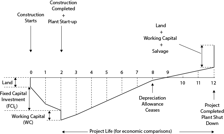
The size of the initial fund and the logic behind the capitalized cost method are illustrated in Figure 10.4.

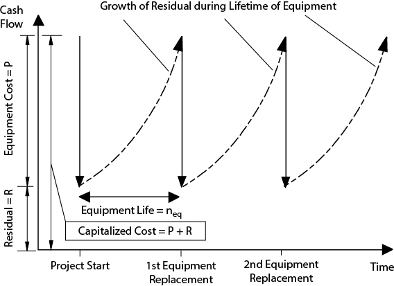
Figure 10.4 An Illustration of the Capitalized Cost Method for the Analysis of Equipment Alternatives

From Figure 10.4, it can be seen that if the equipment replacement cost is P, then the total fund set aside (called the capitalized cost) is P + R, where R is termed the residual. The purpose of this residual is to earn sufficient interest during the life of the equipment to pay for its replacement. At the end of the equipment life, n_eq, the amount of interest earned is P, the equipment replacement cost. As Figure 10.4 shows, replacing the equipment every time it wears out may continue. Referring to Figure 10.4, the equation is developed for the capitalized cost defined as (P + R):

and

The term in square brackets in Equation (10.1) is commonly referred to as the capitalized cost factor.

The capitalized cost obtained from Equation (10.1) does not include the operating cost and is useful in comparing alternatives only when the operating costs of the alternatives are the same. When operating costs vary, it is necessary to capitalize the operating cost. An equivalent capitalized operating cost that converts the operating cost into an equivalent capital cost is added to the capitalized cost calculated from Equation (10.1) to provide the equivalent capitalized cost (ECC):

This cost considers both the capital cost of equipment and the yearly operating cost (YOC) needed to compare alternatives. The extra terms in Equation (10.2) represent the effect of taking the yearly cash flows for operating costs from the residual, R.

By using Equation (10.1) or (10.2), it is possible to account correctly for the different operating lives of the equipment by calculating an effective capitalized cost for the equipment and operating cost. Example 10.7 illustrates the use of these equations.

In Example 10.7, the stainless steel pump costs twice as much as the carbon steel pump and, because of its superior resistance to corrosion, will last nearly twice as long. In addition, the operating cost for the stainless steel pump is lower due to lower maintenance costs. In spite of these advantages, the carbon steel pump was still judged to offer a cost advantage.

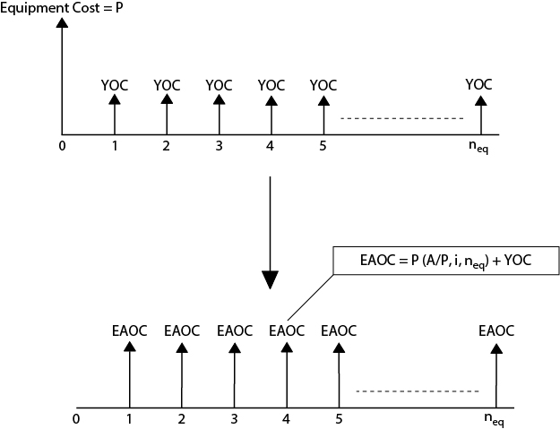
Equivalent Annual Operating Cost (EAOC) Method. In the previous method, both capital cost and yearly operating costs were lumped into a single cash fund or equivalent cash amount. An alternative method is to amortize (spread out) the capital cost of the equipment over the operating life to establish a yearly cost. This is added to the operating cost to yield the EAOC.

Figure 10.5 illustrates the principles behind this method. From Figure 10.5, it can be seen that the cost of the initial purchase will be spread out over the operating life of the equipment. The EAOC is expressed by Equation (10.3):

Figure 10.5 Cash Flow Diagrams Illustrating the Concept of Equivalent Annual Operating Cost

The EAOC method can be understood in terms of the everyday example of comparing new car alternatives. The EAOC can be used to determine whether a higher capital investment, for example, buying a hybrid vehicle, is worthwhile, based on the anticipated savings in the yearly operating cost (reduced fuel consumption).

Example 10.8 illustrates this method for two pumps.

Common Denominator Method. Another method for comparing equipment with unequal operating lives is the common denominator method. This method is illustrated in Figure 10.6, in which two pieces of equipment with operating lives of n and m years are to be compared. This comparison is done over a period of nm years during which the first piece of equipment will need m replacements and the second will require n replacements. Each piece of equipment has an integer number of replacements, and the time over which the comparison is made is the same for both pieces of equipment. For these reasons the comparison can be made using the net present value of each alternative. In general, an integer number of replacements can be made for both pieces of equipment in a time N, where N is the smallest number into which m and n are both exactly divisible; that is, N is the common denominator. Example 10.9 illustrates this method.

Figure 10.6 An Illustration of the Common Denominator Method for the Analysis of Equipment Alternatives

Example 10.9

Compare the two pumps given in Example 10.7 using the common denominator method. The discrete cash flow diagrams for the two pumps are shown in Figure E10.9. The minimum time over which the comparison can be made is 4(7) = 28 years.

Figure E10.9 Cash Flow Diagrams for the Common Denominator Method Used in Example 10.9

Solution

NPV for the carbon steel pump:

NPV	= −($8000)(1 + 1.08−4 + 1.08−8 + 1.08−12 + 1.08−16 + 1.08−20 + 1.08−24)
	−($1800)(P/A, 0.08, 28)
	= −$46,580 (better option)

NPV for the stainless steel pump:

NPV = −($16,000)(1 + 1.08⁻⁷ + 1.08⁻¹⁴ + 1.08⁻²¹) − ($1600)(P/A, 0.08, 28) = −$51,643

The carbon steel pump has a less negative NPV and is recommended.

As found for the previous two methods, the common denominator method favors the carbon steel pump.

Choice of Methods. Because all three methods of comparison correctly take into account the time value of money, the results of all the methods are equivalent. In most problems, the common denominator method becomes unwieldy. The use of the EAOC or the capitalized cost methods are favored for these calculations.

10.6 Incremental Analysis for Retrofitting Facilities

This topic involves profitability criteria used for analyzing situations where a piece of equipment is added to an existing facility. The purpose of adding the equipment is to improve the profitability of the process. Such improvements are often referred to as retrofitting. Such retrofits may be extensive—requiring millions of dollars of investment—or small, requiring an investment of only a few thousand dollars.

The decisions involved in retrofitting projects may be of the discrete type, the continuous type, or a combination of both. An example of a discrete decision is whether to add an on-line monitoring and control system to a wastewater stream. The decision is a simple yes or no. An example of a continuous decision is to determine what size of heat recovery system should be added to an existing process heater to improve fuel efficiency. This type of decision would involve sizing the optimum heat exchanger, where the variable of interest (heat-exchanger area) is continuous.

Because retrofit projects are carried out on existing operating plants, it becomes necessary to identify all of the costs and savings associated with the retrofit. When comparing alternative schemes, the focus of attention is on the profitability of the incremental investment required. Simple, discrete choices will be considered in this section. The problem of optimizing a continuous variable is covered in Chapter 14.

The initial step in an incremental analysis of competing alternatives is to identify the potential alternatives to be considered and to specify the increments over which the analysis is to be performed. The first step is to rank the available alternatives by the magnitude of the capital cost. The alternatives will be identified as A₁, A_2,..., A_n. There are n possible alternatives. The first alternative, A₁, which is always available, is the “do nothing” option. It requires no capital cost (and achieves no savings). For each of the available alternatives, the project cost (capital cost), PC, and the yearly savings generated (yearly cash flow), YS, must be known.

For larger retrofit projects, discounted profitability criteria should be used. The algorithm to compare alternatives using discounted cash flows follows the same four-step method outlined in Section 10.3. For small retrofit projects, nondiscounted criteria may often be sufficiently accurate for comparing alternatives. Both types of criteria are discussed in the next sections.

10.6.1 Nondiscounted Methods for Incremental Analysis

For nondiscounted analyses, two methods are provided below.

1. Rate of Return on Incremental Investment (ROROII)

   ROROII=Incremental Yearly SavingsIncremental Investment

2. Incremental Payback Period (IPBP)

   IPBP=Incremental InvestmentIncremental Yearly Savings

It is observed that these two parameters are reciprocals of each other.

Examples 10.10–10.12 illustrate the method of comparison of projects using these two criteria.

Note that in Part (a) of Example 10.10, the incremental investment and savings are given by the difference between installing the insulation and doing nothing. All of the investments considered in Example 10.10 satisfied the internal benchmark for investment of 15%, which means that the do-nothing option (Option 1) can be discarded. However, which of the remaining options is the best can be determined only by using pairwise comparisons.

It is important to note that in Example 10.11 Options 4 and 5 are rejected even though they give ROROII > 15% when compared with the do-nothing option (see Example 10.10). The key here is that in going from Option 3 to either Option 4 or 5 the incremental investment loses money, that is, ROROII < 15%.

10.6.2 Discounted Methods for Incremental Analysis

Incremental analyses taking into account the time value of money should always be used when large capital investments are being considered. Comparisons may be made either by discounting the operating costs to yield an equivalent capital investment or by amortizing the initial investment to give an equivalent annual operating cost. Both techniques are considered in this section, where the effects of depreciation and taxation are ignored in order to keep the analysis simple. However, it is an easy matter to take these effects into account.

Capital Cost Methods. The incremental net present value (INPV) for a project is given by

When comparing investment options, a given case option will always be compared with a do-nothing option. Thus, these comparisons may be considered as incremental investments. In order to use INPV, it is necessary to know the internal discount rate and the time over which the comparison is to be made. This method is illustrated in Example 10.13.

From the results above, it is clear that Options 2, 3, and 4 are all potentially profitable as INPV > 0. However, the best option is Option 2 because it has the highest INPV when compared with the do-nothing case, Option 1. Note that other pairwise comparisons are unnecessary. The option that yields the highest INPV is chosen. The reason that the INPV gives the best option directly is because by knowing i and n, each dollar of incremental investment is correctly accounted for in the calculation of INPV. Thus, if the incremental investment in going from Option A to Option B is profitable, then the INPV will be greater for Option B and vice versa. It should also be pointed out that by using discounting techniques, the best option has changed from Option 3 (in Example 10.11) to Option 2.

Operating Cost Methods. In the previous section, yearly savings were converted to an equivalent present value using the present value of an annuity, and this was measured against the capital cost. An alternative method is to convert all the investments to annual costs using the capital recovery factor and measure them against the yearly savings.

The needed relationship is developed from Equation (10.4), giving

INPV/(P/A, i, n) = –PC/(P/A, i, n) + YS

It can be seen that the capital recovery factor (A/P,i,n) is the reciprocal of the present worth factor (P/A,i,n). Substituting this relationship and multiplying by −1 gives

–(INPV)(A/P, i, n) = (PC)(A/P, i, n) – YS

The term on the left is identified as the Equivalent Annual Operating Cost (EAOC). Thus,

When an acceptable rate for i and n is substituted, a negative EAOC indicates the investment is acceptable (because a negative cost is the same as a positive savings). Use of EAOC is demonstrated in Example 10.14.

10.7 Evaluation of Risk in Evaluating Profitability

In this section, the concept of risk in the evaluation of profitability is introduced, and the techniques to quantify it are illustrated. Until now, it has been assumed that the financial analysis is essentially deterministic—that is, all factors are known with absolute certainty. Recalling discussions in Chapter 7 regarding the relative error associated with capital cost estimates, it should not be surprising that many of the costs and parameters used in evaluating the profitability of a chemical process are estimates that are subject to error. In fact, nearly all of these factors are subject to change throughout the life of the chemical plant. The question then is not, “Do these parameters change?” but rather, “By how much do they change?” In Table 10.1, due to Humphreys [1], ranges of expected variations for factors that affect the prediction and forecasting of profitability are given.

The most important variable in Table 10.1 is sales volume, with the price of product and raw material being a close second. Clearly, if market forces were such that it was possible to sell (and hence produce) only 50% of the originally estimated amount of product, then profitability would be affected greatly. Indeed, the process would quite possibly be unprofitable. The problem is that projections of how the variables will vary over the life of the plant are difficult (and sometime impossible) to estimate. Nevertheless, experienced cost estimators often have a feel for the variability of some of these parameters. In addition, marketing and financial specialists within large companies have expertise in forecasting trends in product demand, product price, and raw material costs. In the next section, the effect that supply and demand have on the sales price of a product is investigated. Following this, methods to quantify risk and to predict the range of profitability that can be expected from a process, when uncertainty exists in some of the profitability parameters listed in Table 10.1, will be discussed.

10.7.1 Forecasting Uncertainty in Chemical Processes

In order to be able to predict the way in which the factors in Table 10.1 vary, it is necessary to take historical data along with information about new developments to formulate a model to predict trends in key economic parameters over the projected life of a process. This prediction process is often referred to as forecasting and is, in general, a very inexact science. The purpose of this section is to introduce some concepts that must be considered when quantifying economic projections. A detailed description of the art of economic forecasting is way beyond the scope of this text. Instead, the basic concepts and factors influencing economic parameters are introduced.

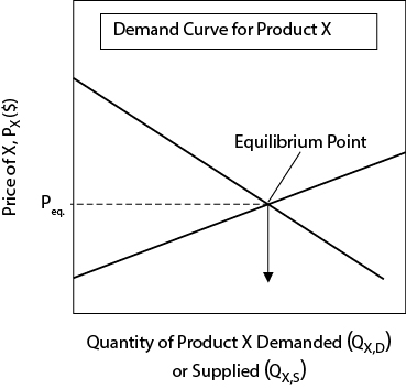
Supply and Demand Concepts in Chemical Markets. Economists use microeconomic theory [2] to describe how changes in the supply of and demand for a given product are affected by changes in the market. Only the most basic supply and demand curves, shown in Figure 10.7, are considered here.

Figure 10.7 Simple Supply and Demand Curves for Product X

The demand curve (on the left) slopes downward and shows the general trend that as the price for commodity X decreases, the demand increases. With very few exceptions, this is always true. Examples of chemical products following this trend are numerous; for example, as the price of gasoline, polyethylene, or fertilizer drops, the demand for these goods increases (all other factors remaining constant). The supply curve (shown on the right) slopes upward and shows the trend that as the price rises, the amount of product X that manufacturers are willing to produce increases. The slope of the supply curve is often positive but may also be negative depending on the product. For most chemical products, it can be assumed that the slope is positive, and with all other factors remaining constant, the quantity supplied increases as the price for the product increases. Unlike physical laws that govern thermodynamics, heat transfer, and so on, these trends are not absolute. Instead, these trends reflect human nature relating to buying and selling of goods.

When market forces are in equilibrium, the supply and demand for a given product are balanced, and the equilibrium price (P_eq) is determined by the intersection of the supply and demand curves, as shown in Figure 10.8.

Figure 10.8 Illustration of Market Equilibrium for Product X

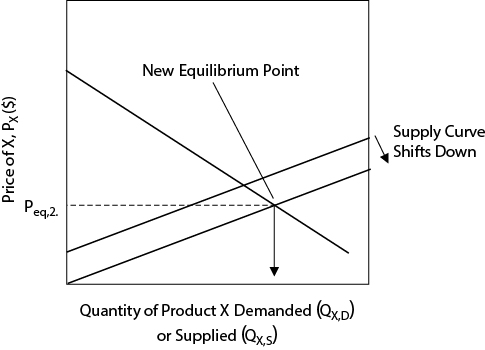
There are many factors that can affect the market for product X. Indeed, a market may not be in equilibrium, and, in this case, the market price must be determined in terms of rate equations as opposed to equilibrium relationships. However, for the sake of this simplified discussion, it will be assumed that market equilibrium is always reached. If something changes in the market, either the supply or demand curve (or both) will shift, and a new equilibrium point will be reached. As an example, consider the situation when a large new plant that produces X comes on line. Assuming that nothing else in the market changes, the supply curve will be shifted downward and to the right, which will lead to a lower equilibrium price. This situation is illustrated in Figure 10.9. The intersection of the demand curve and the new supply curve gives rise to the new equilibrium price, P_eq,2, which is lower than the original equilibrium price, P_eq,1. The magnitude of the decrease in the equilibrium price depends on the magnitude of the downward shift in the supply curve. If the new plant is large compared with the total current manufacturing capacity for product X, then the decrease in the equilibrium price will be correspondingly large. If this decrease in price is not taken into account in the economic analysis, the projected profitability of the new project will be overestimated, and the decision to invest might be made when the correct decision would be to abandon the project.

Figure 10.9 Illustration of Market Equilibrium for Product X When a New Plant Comes on Line

The situation is further complicated when competing products are considered. For example, if product Y can be used as a substitute for product X in some applications, then factors that affect Y will also affect X. It is easy to see that quantifying and predicting changes become very difficult. Torries [3] identifies important factors that affect both the shape and relative location of the supply and demand curves. These factors are listed in Table 10.2.

In order to forecast accurately the prices of a product over a 10- or 15-year project, the factors in Table 10.2 need to be predicted. Clearly, even for the most well-known and stable products, this can be a daunting task. An alternative method to quantifying the individual supply and demand curves is to look at historical data for the product of interest.

The examination of historical data is a convenient way to obtain general trends in pricing. Such data represent the change in equilibrium price for a product with time. Often such data fluctuate widely, and although long-term trends may be apparent, predictions for the next one or two years will often be wildly inaccurate. For example, consider the data for average gasoline prices over the period January 1995 to June 2016, as shown in Figure 10.10. The straight line is a regression through the data and represents the best linear fit of the data. If this were the forecast for gasoline prices over this period, it would be a remarkably good prediction. However, even with this predicting line, significant variations in actual product selling price are noted. The maximum positive and negative deviations are +75¢/gal (+30%) and −45¢/gal (−24%). To illustrate further the effect of these deviations on profitability calculations, consider a new refinery starting production in late 2012. For this new plant, the selling price for its major product (gasoline) over the four-year period after start-up drops by $1.45/gal. If this refinery were contracted to buy crude oil at a price fixed previously, then the profitability of the plant over this initial four-year period would be severely diminished and it would probably lose money.

Figure 10.10 Average Price of All Grades of Gasoline over the Period January 1995 to June 2016 (from www.eia.doe.gov)

From the brief discussion given above, it is clear that predicting or forecasting future prices for chemical products is a very inexact and risky business. Perhaps it is best summed up by a quote attributed to “baseball philosopher” Yogi Berra [4]:

In the following section, it will be assumed that such predictions are available and will be used as given, known quantities. The question then is how much meaning can be placed on the results of these predictions when the input data—the basic variability of the parameters—is often poorly known. The answer is that by investigating and looking at how these parameters affect profitability, a better picture of how this variability or uncertainty affects the overall profitability of a project can be obtained. In general, this type of information is much more useful than the single-point estimate of profitability that has been considered up to this point.

10.7.2 Quantifying Risk

It should be noted that the quantification of risk in no way eliminates uncertainty. Rather, by quantifying it, a better feel can be developed for how a project’s profitability may vary. Therefore, more informed and rational decisions regarding whether to build a new plant can be made. However, the ultimate decision to invest in a new chemical process always involves some element of risk.

Scenario Analysis. Returning to Example 10.1 regarding the profitability analysis for a new chemical plant, assume that, as the result of previous experience with similar chemicals and some forecasting of supply and demand for this new product, it is believed that the product price may vary in the range –20% to +5%, the capital investment may vary between –20% and +30%, and the cost of manufacturing may vary in the range –10% to +10%. How can these uncertainties be quantified?

One way to quantify uncertainty is via a scenario analysis. In this analysis, the best- and worst-case scenarios are considered and compared with the base case, which has already been calculated. The values for the three parameters for the two cases are given in Table 10.3.

Next, these values are substituted into the spreadsheet shown in Table E10.1, and all the cash flows are discounted back to the start of the project to estimate the NPV. The results of these calculations are shown in Table 10.4.

The results in Table 10.4 show that, in the worst-case scenario, the NPV is very negative and the project will lose money. In the best-case scenario, the NPV is increased over the base case by approximately $35 million. From this result, the decision on whether to go ahead and build the plant is not obvious. On one hand, the process could be highly profitable, but on the other hand, it could lose nearly $60 million over the course of the ten-year plant life. By taking a very conservative philosophy, the results of the worst-case scenario suggest a decision of “do not invest.” However, is the worst-case scenario realistic? Most likely, the worst-case (best-case) scenario is unduly pessimistic (optimistic). Consider each of the three parameters in Table 10.3. It will be assumed that the value of the parameter has an equal chance of being at the high, base-case, or low value. Therefore, in terms of probabilities, the chance of the parameter taking each of these values is 1/3, or 33.3%. Because there are three parameters (R, FCI_L, and COM_d), each of which can take one of three values (high, base case, low), there are 3³ = 27 combinations as shown in Table 10.5.

From Table 10.5, it can be seen that Scenario 9 is the worst case and Scenario 19 is the best case. Either of these two cases has a 1 in 27 (or 3.7%) chance of occurring. Based on this result, it is not very likely that either of these scenarios would occur, so care should be taken in evaluating the scenario analysis. This is indeed one of the main shortcomings of the scenario analysis [2]. In reviewing Table 10.5, a better measure of the expected profitability might be the weighted average of all 27 possible outcomes. The idea of weighting results based on the likelihood of occurrence is the basis of the probabilistic approach to quantifying risk that will be discussed shortly. However, before looking at that method, it is instructive to determine the sensitivity of the profitability of the project to changes in important parameters. Sensitivity analysis is covered in the next section.

Sensitivity Analysis. To a great extent, the risk associated with the variability of a given parameter is dependent on the effect that a change in that parameter has on the profitability criterion of interest. For the sake of this discussion, the NPV will be used as the measure of profitability. However, this measure could just as easily be the DCFROR, DPEP, or any other profitability criterion discussed in Section 10.2. If it is assumed that the NPV is affected by n parameters (x₁, x₂, x₃, …, x_n), then the first-order sensitivity to parameter x₁ is given in mathematical terms by the following quantity:

where the partial derivative is taken with respect to x₁, while holding all other parameters constant at their mean value. The sensitivity, S₁, is sometimes called a sensitivity coefficient. In general, this quantity is too complicated to obtain via analytical differentiation; hence, it is obtained by changing the parameter by a small amount and observing the subsequent change in the NPV, or

In Example 10.15, Example 10.1 is revisited to illustrate how the sensitivities of the revenue, cost of manufacturing, and fixed capital investment on the NPV are calculated.

Example 10.15

For the chemical process considered in Example 10.1, calculate the sensitivity of R, COM_d, and FCI_L and plot these sensitivities with respect to the NPV.

Solution

The effect of a 1% change is considered (½% on either side of the base case) in each parameter on the NPV. These results are shown in Table E10.15.

Table E10.15 Calculations for Sensitivity Analysis for Example 10.1 (All $ Figures Are in Millions)

Parameter	Value	NPV	Value	NPV	Si
x1 (Revenue, R)	+0.5% ($75.375/y)	$18.17	−0.5% ($74.625/y)	$16.07	(18.17−16.07)(75.375−74.625)=2.10.75=2.80 y
x2 (COMd)	+0.5% ($30.150/y)	$16.70	−0.5% ($29.850/y)	$17.54	(16.70−17.54)(30.15−29.85)=−0.840.30=−2.80 y
x3 (FCIL)	+0.5% ($150.75)	$16.68	−0.5% ($149.25)	$17.56	(16.68−17.56)(150.75−149.25)=−0.881.50=−0.59 y

The fact that S₁ = −S₂ should not be surprising because, in the calculation of yearly cash flows, whenever R appears COM_d is subtracted from it (see Table E10.1). The changes in NPV for percent changes in each parameter are illustrated in Figure E10.15. The slopes of the lines are not equal to the sensitivities, because the x-axis is the percent change rather than the actual change in the parameter.

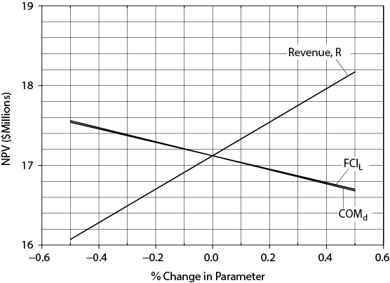
Figure E10.15 Sensitivity Curves for the Parameters Considered in Example 10.15

How can the sensitivity values calculated in Example 10.15 be used to estimate changes in the profitability criterion of the process? For small changes in the parameters, it may be assumed that the sensitivities are constant and can be added. Therefore, the change in NPV can be predicted for a set of changes in the parameters using the relationship in Equation (10.8):

Example 10.16 illustrates this concept.

A Probabilistic Approach to Quantifying Risk: The Monte-Carlo Method. The basic approach adopted here will involve the following steps:

1. All parameters for which uncertainty is to be quantified are identified.

2. Probability distributions are assigned for all parameters in Step 1.

3. A random number is assigned for each parameter in Step 1.

4. Using the random number from Step 3, the value of the parameter is assigned using the probability distribution (from Step 2) for that parameter.

5. Once values have been assigned to all parameters, these values are used to calculate the profitability (NPV or other criterion) of the project.

6. Steps 3, 4, and 5 are repeated many times (for example, 1000).

7. A histogram and cumulative probability curve for the profitability criteria calculated from Step 6 are created.

8. The results of Step 7 are used to analyze the profitability of the project.

The algorithm described in this eight-step process is best illustrated by means of an example. However, before these steps can be completed, it is necessary to review some basic probability theory.

Probability, Probability Distribution, and Cumulative Distribution Functions. A detailed analysis and description of probability theory are beyond the scope of this book. Instead, some of the basic concepts and simple distributions are presented. The interested reader is referred to Resnick [5], Valle-Riestra [6], and Rose [7] for further coverage of this subject.

For any given parameter for which uncertainty exists (and to which some form of distribution will be assigned), the uncertainty must be described via a probability distribution. The simplest distribution to use is a uniform distribution, which is illustrated in Figure 10.11.

Figure 10.11 Uniform Probability Density Function

From Figure 10.11, the parameter of interest can take on any value between a and b with equal likelihood. Because the uniform distribution is a probability density function, the area under the curve must equal 1, and hence the value of the frequency (y-axis) is equal to 1/(b–a). The probability density function can be integrated to give the cumulative probability distribution, which for the uniform distribution is given in Figure 10.12.

Figure 10.12 Cumulative Probability Distribution for a Uniform Probability Density Function

Figure 10.12 is interpreted by realizing that the probability of the parameter being less than or equal to x is P. Alternatively, a random, uniformly distributed value of the parameter can be assigned by choosing a random number in the range 0 to 1 (on the y-axis) and reading the corresponding value of the parameter, between a and b, on the x-axis. For example, if the random number chosen is P, then, using Figure 10.12, the corresponding value of the parameter is x. Clearly, the shapes of the density function and the corresponding cumulative distribution influence the values of the parameters that are used in the eight-step algorithm. Which probability density function should be used? Clearly, if frequency occurrence data for a given parameter are available, the distribution can be constructed. However, complete information about the way in which a given parameter will vary is often not available. The minimum data set would be the most likely value (b), and estimates of the highest (c) and lowest (a) values that the parameter could reasonably take. With this information, a triangular probability density function or distribution, shown in Figure 10.13, can be constructed. The corresponding cumulative distribution is shown in Figure 10.14. The equations describing these distributions are as follows:

Figure 10.13 Probability Density Function for Triangular Distribution

Figure 10.14 Cumulative Probability Function for Triangular Distribution

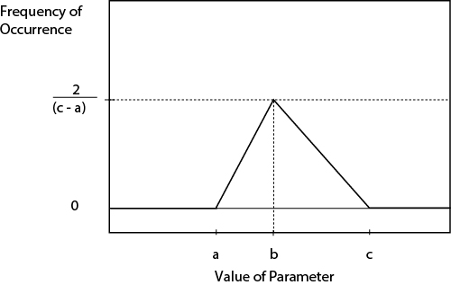
Triangular probability density function:

Triangular cumulative probability function:

Clearly, any probability density function and corresponding cumulative probability distribution could be used to describe the uncertainty in the data. Trapezoidal, normal, lognormal, and so on, are used routinely to describe uncertainty in data. However, for simplicity, the following discussions are confined to triangular distributions. The eight-step method for quantifying uncertainty in profitability analysis is illustrated next.

Monte-Carlo Simulation. The Monte-Carlo (M-C) method is simply the concept of assigning probability distributions to parameters, repeatedly choosing variables from these distributions, and using these values to calculate a function dependent on the variables. The resulting distribution of calculated values of the dependent function is the result of the M-C simulation. Therefore, the eight-step procedure is simply a specific case of the M-C method. Each of the eight steps is illustrated using the example discussed previously in the scenario analysis.

Step 1: All the parameters for which uncertainty is to be quantified are identified. Returning to Example 10.1, historical data suggest that there is uncertainty in the predictions for revenue (R), cost of manufacturing (COM_d), and fixed capital investment (FCI_L).

Step 2: Probability distributions are assigned for all parameters in Step 1. All the uncertainties associated with these parameters are assumed to follow triangular distributions with the properties given in Table 10.6.

Step 3: A random number is assigned for each parameter in Step 1. First, random numbers between 0 and 1 are chosen for each variable. The easiest way to generate random numbers is to use the Rand() function in Microsoft’s Excel program or a similar spreadsheet. Tables of random numbers are also available in standard math handbooks [8].

Step 4: Using the random number from Step 3, the value of the parameter is assigned using the probability distribution (from Step 2) for that parameter. With the value of the random number equal to the right-hand side of Equation (10.10) and using the corresponding values of a, b, and c, this equation is solved for the value of x. The value of x is the value of the parameter to use in the next step. Table 10.7 illustrates this procedure for R, COM_d, and FCI_L.

To illustrate how the random values for the parameters are obtained, consider the calculation for COM_d. The number 0.6498 was chosen at random from a uniform distribution in the range 0–1 using Microsoft’s Excel spreadsheet. This number, along with values of a = 27, b = 30, and c = 33, are then substituted for P(x) in Equation (10.10) to give

From Equation (10.10), the P(x) value for x = b is given by

Because the value of the random number (0.6498) is greater than 0.5, the form of the equation for x > b must be used. Solving for x yields

Step 5: Once values have been assigned to all parameters, these values are used to calculate the profitability (NPV or other criterion) of the project. The spreadsheet given in Table E10.1 was used to determine the NPV using the values given in Table 10.7. The NPV is also shown in Table 10.7.

Step 6: Steps 3, 4, and 5 are repeated many times (say, 1000). For the sake of illustration, Steps 3, 4, and 5 were repeated 20 times to yield 20 values of the NPV. These results are summarized in Table 10.8.

Step 7: A histogram or cumulative probability curve is created for the values of the profitability criterion calculated from Step 6. Using the data from Table 10.8, a cumulative probability curve is constructed. To do this, the data are ordered from lowest (−28.20) to highest (28.27), and the cumulative probability of the NPV being less than or equal to the value on the x-axis is plotted. The results are shown in Figure 10.15. The dashed line simply connects the 20 data points for this simulation. This line shows several bumps that are due to the small number of simulations. The solid line represents the data for 1000 simulations, and it can be seen that this curve is essentially smooth. The 1000-point simulation was carried out using the CAPCOST software accompanying the text. The use of the software is addressed at the end of this section.

Figure 10.15 Cumulative Probability of NPV for Monte-Carlo Simulation

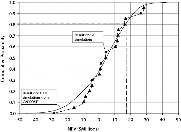
Step 8: The results of Step 7 are used to analyze the profitability of the project. From Figure 10.15, it can be seen that there is about a 38% chance that the project will not be profitable. The median NPV is about $5 million, and only about 21% of the values calculated lie above $17.12 million, which is the NPV calculated for the base case, using the most likely values of R, COM_d, and FCI_L.

Another way that the data from an M-C analysis can be used is in the comparison of alternatives. For example, consider two competing projects, A and B. A probabilistic analysis of both these projects yields the data shown in Figure 10.16. If only the median profitability is considered, corresponding to a cumulative probability of 0.5, then it might be concluded that Project A is better. Indeed, over a wide range of probabilities Alternative A gives a higher NPV than Alternative B. However, this type of comparison does not give the whole picture. By looking at the low end of NPV predictions, it is found that Project A has a 17% chance of returning a negative NPV compared with Project B, which is predicted to have only a 2% chance of giving a negative NPV. Clearly, the choice regarding Projects A and B must be made taking into account both the probability of success and the magnitude of the profitability. The Monte-Carlo analysis allows a far more complete financial picture to be painted, and the decisions from such information will be more profound having taken more information into account.

Figure 10.16 A Comparison of the Profitability of Two Projects Showing the NPV with Respect to the Estimated Cumulative Probability from a Monte-Carlo Analysis

Evaluation of the Risks Associated with Using New Technology. To this point, risks associated with predicting the items listed in Table 10.1 have been considered. For example, predictions for the variations associated with the cost of the plant, the cost of manufacturing, and the revenue generated by the plant were made. Then, by using the M-C technique, the relationship given in Figure 10.15 was generated. For processes using new technology, additional risks will be present, but these risks may be impossible to quantify in terms of the parameters given in Table 10.1. One way to take this additional risk into account is to assign a higher acceptable rate of return for projects using new technology compared with those using mature technologies. The effect of using a higher discount rate is to move the curve in Figure 10.15 to the left. This is illustrated in Figure 10.17. From this figure, it is apparent that if an acceptable rate of return is 15% p.a., then the project is not acceptable, whereas at a rate of 10% p.a. the project looks quite favorable. It can be argued that using a higher hurdle rate for new processes is unnecessary, because, for a new project, there will be greater ranges in the predictions of the variables, and this automatically makes the project using new technology “riskier,” as the effect of broader ranges for variables is to flatten the NPV-probability curve. However, it may be impossible to estimate the effect of the new technology on, for example, the cost of manufacturing or the acceptance of a new product in the market. By specifying a higher acceptable rate of return on the investment for these projects, the interpretation between projects using new and old technologies is clear and unambiguous.

Figure 10.17 The Effect of Interest (Hurdle) Rate on Monte-Carlo Simulations

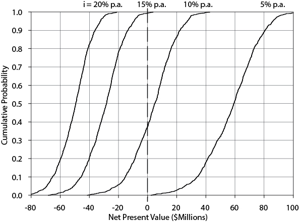
Monte-Carlo Analysis Using CAPCOST. The CAPCOST program introduced in Chapter 7 includes spreadsheets for estimating the cash flows of a project and the evaluation of profitability criteria such as NPV and DCFROR. In addition, a Monte-Carlo simulation has also been included that allows the following variables to be investigated:

• FCI_L

• Price of product

• Working capital

• Income tax rate

• Interest rate

• Raw material price

• Salvage value

By specifying the ranges over which these terms are likely to vary, a Monte-Carlo analysis for a given problem can be achieved. Distributions of criteria such as NPV and DPBP are automatically given. The reader should consult the help file on the website for a tutorial on the use of this software.

10.8 Profit Margin Analysis

All the techniques that have been discussed in this chapter use the fixed capital cost and the operating costs to evaluate the profitability of a process. Clearly, the accuracy of such predictions depends on the accuracy of the estimates for the different costs. When screening alternative processes, it is sometimes useful to evaluate the difference between the revenue from the sale of products and the cost of raw materials. This difference is called the profit margin or sometimes just the margin.

If the profit margin is negative, the process will never be profitable. This is because no capital cost, utility costs, and other ancillary operating costs have been taken into account. A positive profit margin does not guarantee that the process will be profitable but does suggest that further investigation may be warranted. Therefore, the profit margin is a useful, but limited, tool for the initial screening of process alternatives. This is illustrated in Example 10.17.

Clearly, from an analysis of the profit margin, further investigation of the maleic anhydride process is not warranted.

10.9 Summary

In this chapter, the basics of profitability analysis for projects involving large capital expenditures were covered. The concepts of nondiscounted and discounted profitability criteria were introduced, as were the three bases for these criteria: time, money, and interest rate.

How to choose the economically optimum piece of equipment among a group of alternatives using the capitalized cost, the equivalent annual operating cost, and the common denominator methods was demonstrated.

The concept of incremental economic analysis was introduced and applied to an example involving large capital budgets and also to a retrofit project. It was shown that both the net present value (NPV) and the equivalent annual operating cost (EAOC) methods were particularly useful when comparing alternatives using discounted cash flows.

Finally, the concept of assigning probabilities to variables in order to quantify risk was discussed. The Monte-Carlo technique was introduced, and its application to simulate the cumulative distribution of net present values of a project was described. The interpretation of results from this technique was presented. Finally, the simulation of risk and the analysis of data using the CAPCOST package was illustrated by an example.

References

1. Humphreys, K. K., Jelen’s Cost and Optimization Engineering, 3rd ed. (New York: McGraw-Hill, 1991).

2. Salvatore, D., Schaum’s Outline of Theory and Problems of Microeconomic Theory, 3rd ed. (New York: McGraw-Hill, 1992).

3. Torries, T. F., Evaluating Mineral Projects: Applications and Misconceptions (Littleton: SME, 1998).

4. http://en.wikiquote.org/wiki/Yogi_Berra.

5. Resnick, W., Process Analysis and Design for Chemical Engineers (New York: McGraw-Hill, 1981).

6. Valle-Riestra, J. F., Project Evaluation in the Chemical Process Industries (New York: McGraw-Hill, 1983).

7. Rose, L. M., Engineering Investment Decisions: Planning under Uncertainty (Amsterdam: Elsevier, 1976).

8. Spiegel, M. R., Mathematical Handbook of Formulas and Tables, Schaum’s Outline Series (New York: McGraw-Hill, 1968).

Short Answer Questions

1. The evaluation of a project requiring a large capital investment has yielded an NPV (net present value) of $20 × 10⁶. If the internal hurdle rate for this project was set at 10% p.a., will the DCFROR (discounted cash flow rate of return) be greater or less than 10%? Explain.

2. The following are results of a recent evaluation of two projects. Which would you choose? Defend your choice. Your opportunity cost for capital is 15%.

3. Explain the concept of an incremental economic analysis.

4. When comparing two pieces of equipment for a given service, if each piece of equipment has the same life and each costs the same, would the amount of maintenance required for the equipment be an important factor? Why?

5. What economic criterion would you use to choose the best piece of equipment among three alternatives, each with a different operating cost, capital cost, and equipment life?

6. Do you agree with the statement “Monte-Carlo simulation enables the design engineer to eliminate risk in economic analysis”? Please explain your answer.

7. In evaluating a large project, what are the advantages and disadvantages of probabilistic analysis?

Problems

For the following problems, unless stated otherwise, you may assume that the cost of land, L, and the salvage value, S, of the plant are both zero.

8. The projected costs for a new plant are given below (all numbers are in $10⁶).

Land cost = $7.5

Fixed capital investment = $120 ($60 at end of year 1, $39.60 at end of year 2, and $20.40 at end of year 3)

Working capital = $35 (at start-up)

Start-up at end of year 3

Revenue from sales = $52

Cost of manufacturing (without depreciation) = $18

Tax rate = 40%

Depreciation method = MACRS over 5 years

Length of time over which profitability is to be assessed = 10 years after start-up

Internal rate of return = 9.5% p.a.

For this project, do the following:

1. Draw a cumulative (nondiscounted) after-tax cash flow diagram.

2. From Part (a), calculate the following nondiscounted profitability criteria for the project:

   1. Cumulative cash position and cumulative cash ratio

   2. Payback period

   3. Rate of return on investment

3. Draw a cumulative (discounted) after-tax cash flow diagram.

4. From Part (c), calculate the following discounted profitability criteria for the project:

   1. Net present value and net present value ratio

   2. Discounted payback period

   3. Discounted cash flow rate of return (DCFROR)

9. Repeat Problem 10.8 using a straight-line depreciation method over 7 years. Compare the results with those obtained in Problem 10.8. Which depreciation method would you use?

10. The following expenses and revenues have been estimated for a new project:

Revenues from sales = $4.1 × 10⁶/y

Cost of manufacturing (excluding depreciation) = $1.9 × 10⁶/y

Taxation rate = 40%

Fixed capital investment = $7.7 × 10⁶

(two payments of $5 × 10⁶ and $2.7 × 10⁶ at the end of years 1 and 2, respectively)

Start-up at the end of year 2

Working capital = $2 × 10⁶ at the end of year 2

Land cost = $0.8 × 10⁶ at the beginning of the project (time = 0)

Project life (for economic evaluation) = 10 y after start-up

For this project, estimate the NPV of the project assuming an after-tax internal hurdle rate of 11% p.a., using the following depreciation schedules:

1. MACRS method for 5 years

2. Straight-line depreciation with an equipment life (for depreciation) of 9.5 years

Comment on the effect of discounting on the overall profitability of large capital projects.

11. In reviewing current operating processes, the company accountant has provided you with the following information about a small chemical process that was built ten years ago.

Capital investment = $30 × 10⁶ ($10 × 10⁶ at the end of year 1, $15 × 10⁶ at the end of year 2, $5 × 10⁶ at the end of year 3. Working capital = $10 × 10⁶)

Over the last ten years, the average (after-tax) return on investment that nonprocess projects have yielded is 10%.

1. What is the DCFROR for this project over the last 12 years? (Ignore land and working capital costs.)

2. In retrospect, was the decision to build this plant a good one?

12. The after-tax cash flows for a new chemical process are shown in Table P10.12. Using these data, calculate the following:

1. Payback period (PBP)

2. Cumulative cash position (CCP) and cumulative cash ratio (CCR)

3. Rate of return on investment (ROROI)

4. Discounted payback period (DPBP)

5. Net present value (NPV)

6. Discounted cash flow rate of return (DCFROR)

Use a 10% discount rate for Parts (d) and (e).

13. From the data given in Table P10.12, determine the following information regarding the calculations performed for this analysis:

1. What taxation rate was assumed?

2. What was the total fixed capital investment?

3. What method of depreciation was used?

4. What was the cost of manufacturing, not including depreciation?

14. Consider the following two new chemical plants, each with an initial fixed capital investment (year 0) of $15 × 10⁶. Their cash flows are as follows:

1. Calculate the NPV of both plants for interest rates of 6% and 18%. Which plant do you recommend? Explain your results.

2. Calculate the DCFROR for each plant. Which plant do you recommend?

3. Calculate the nondiscounted payback period (PBP) for each plant. Which plant do you recommend?

4. Explain any differences in your answers to Parts (a), (b), and (c).

15. In a design, you have the choice of purchasing one of the following batch reactors:

If the internal rate of return for such comparisons is 9% p.a., which of the alternatives is least costly?

16. Two pieces of equipment are being considered for an identical service. The installed costs and yearly operating costs associated with each piece of equipment are as follows:

1. If the internal hurdle rate for comparison of alternatives is set at 15% p.a., which piece of equipment do you recommend be purchased?

2. Above what internal hurdle rate would you recommend Project A?

17. Your company is considering modifying an existing distillation column. A new reboiler and condenser will be required, along with several other peripherals. The equipment lists are as follows:

The internal hurdle rate for comparison of investments is set at 12% p.a. Which option do you recommend?

18. Because of corrosion, the feed pump to a batch reactor must be replaced every three years. What is the capitalized cost of the pump?

Data:

19. Three alternative pieces of equipment are being considered for solids separation from a liquid slurry:

If the internal hurdle rate for this project is 11% p.a., which alternative do you recommend?

20. A change in air pollution control equipment is being considered. A baghouse filter is being considered to replace an existing electrostatic precipitator. Consider the costs and savings for the project in the following data:

Should the baghouse filter be purchased and installed?

21. In considering investments in large capital projects, a company is deciding in which of the following projects it will invest:

The company can always invest its money in stocks that are expected to yield 5.5% p.a. (after tax). In which, if any, of the projects should the company invest if the capital ceiling for investment is $250 million and a project life of 10 years is assumed? Would you argue to raise the investment ceiling?

22. Because you live in a southern, warm-weather climate, your electricity bill is very large for about eight months of the year due to the need for air conditioning. You have been approached by an agency that would like to assist you in installing solar panels to provide electricity to run your air conditioning. You were also considering adding additional insulation to your house. You also have the option of doing nothing. Which of the following options would you choose based on the given data?

1. Do nothing.

2. Install only the solar collector.

3. Install only the insulation.

4. Install both the solar collector and the insulation.

Data (all figures in $thousands)

If there were a tax credit for installing the solar collector in the year in which it was installed, how much of a tax credit (in % of initial investment) would be required to make the solar collector alone a worthwhile investment?

23. You have been asked to evaluate several investment opportunities for the biotechnology company for which you work. These potential investments concern a new process to manufacture a new, genetically engineered pharmaceutical. The financial information on the process alternatives are as follows:

For the alternatives, the capital investment and the yearly after-tax cash flows are incremental to the base case. The assumed plant life is 12 years, and all of the capital investment occurs at time = 0.

1. If an acceptable, nondiscounted rate of return on investment (ROROI) is 25% p.a., which is the best option?

2. If an acceptable, after-tax, discounted rate of return is 15% p.a., which option is the best?

24. Your company is considering investing in a process improvement that would require an initial capital investment of $500,000. The projected increases in revenue over the next seven years are as follows:

1. The company can always leave the capital investment in the stock portfolio, which is projected to yield 8% p.a. over the next seven years. What should the company do?

2. What is the break-even rate of return between the process improvement and doing nothing?

3. If the capital investment could be changed without changing the incremental revenues, what capital investment changes this investment from being profitable (not profitable) to being not profitable (profitable)?

25. During the design of a new process to manufacture nanocomposites, several alternative waste treatment processes are being considered. The base case is the main waste treatment process, and the options are modifications to the base case. Not all options are compatible with each other, and the economic data on the only possible combinations are as follows:

The nondiscounted, internal hurdle rate for investment is 14% p.a., after tax. Which waste treatment process do you recommend?

26. The installation of a new heat exchanger is proposed for the batch crystallization step in an existing pharmaceutical manufacturing process. The heat exchanger costs $49,600 (installed) and saves $8000/y in operating costs. Is this a good investment based on a before-tax analysis?

Data:

27. A process for the fabrication of microelectronic components has been designed. The required before-tax return on investment is 18% p.a., and the equipment life is assumed to be eight years.

1. Do you recommend construction of the base-case process?

2. Do you recommend including either of the process alternatives?

3. Suppose there were another alternative, compatible with either of the previous alternatives, requiring an additional $3.26 million capital investment. What savings in operating cost would be required to make this alternative economically attractive?

28. A new pharmaceutical plant is expected to cost (FCI_L) $25 million, and the revenue (R) from the sale of products is expected to be $10 million/y for the first four years of operation and $15 million/y thereafter. The cost of manufacturing without depreciation (COM_d) is projected to be $4 million/y for the first four years and $6 million/y thereafter. The cost of land (at the end of year zero) is $3 million, the working capital at start-up (which occurs at the end of year 2) is $3 million, and the fixed capital investment is assumed to be paid out as $15 million at the end of year 1 and $10 million at the end of year 2. Yearly income starts in year 3, and the plant life is ten years after start-up. The before-tax criterion for profitability is 17%. Assume the plant has no salvage value, but that the cost of land and the working capital are recovered at the end of the project life.

1. Draw a labeled, discrete, nondiscounted cash flow diagram for this project.

2. Draw a labeled, cumulative, discounted (to year zero) cash flow diagram for this project.

3. What is the NPV for this project? Do you recommend construction of this plant?

29. How much would you need to save annually to be willing to invest $1.75 million in a process improvement? The internal hurdle rate for process improvements is 18% before taxes over eight years.

30. How much would you be willing to invest in a process improvement to save $2.25 million/y? The internal hurdle rate for process improvements is 15% before taxes over six years.

31. You can invest $5.1 million in a process improvement to save $0.9 million/y. What internal hurdle rate would make this an attractive option? The assumed lifetime for these improvements is nine years.

32. Recommend whether your company should invest in the following process: The internal hurdle rate is 17% p.a., before taxes, over an operating lifetime of 12 years. The fixed capital investment is made in two installments: $5 million at time zero and $3 million at the end of year 1. At the end of year 1, $1 million in working capital is required. For the remainder of the project lifetime, $2 million in income is realized.

33. You are considering two possible modifications to an existing microelectronics facility. The criterion for profitability is 18% p.a. over six years. All values are in $million.

1. What do you recommend based on a nondiscounted ROROII analysis?

2. What do you recommend based on an INPV analysis?

3. Based on the results of Parts (a) and (b), what do you recommend?

34. A new biotech plant is expected to cost (FCI_L) $20 million, with $10 million paid at the beginning of the project and $10 million paid at the end of year 1. There is no land cost because the land is already owned. The annual profit, before taxes, is $4 million and the working capital at start-up (which occurs at the end of year 1) is $1 million. The plant life is 10 years after start-up. The before-tax criterion for profitability is 12%. Assume that the plant has no salvage value, and that the working capital is recovered at the end of the project life.

1. Draw a labeled, discrete, nondiscounted cash flow diagram for this project.

2. Draw a labeled, cumulative, discounted (to year zero) cash flow diagram for this project.

3. What is the NPV for this project? Do you recommend construction of this plant?

4. What would the annual profit, before taxes, have to be for the NPV to be $2 million?

5. The plant is built and has been operational for several years. It has been suggested that $3 million be spent on plant modifications that will save money. Your job is to analyze the suggestion. The criterion for plant modifications is a 16% before-tax return over five years. How much annual savings are required before you would recommend in favor of investing in the modification?

35. You are responsible for equipment selection for a new micro-fiber process. A batch blending tank is required for corrosive service. You are considering three alternatives:

The after-tax internal hurdle rate is 14% p.a. Which alternative do you recommend?

36. In an already operational pharmaceutical plant, you are considering three alternative solvent-recovery systems to replace an existing combustion process. The internal hurdle rate is 15% after taxes over eight years. Which alternative do you recommend?

37. A condenser using refrigerated water is being considered for the recovery of a solvent used in a pharmaceutical coating operation. The amount of solvent recovered from the gas stream is a function of the temperature to which it is cooled. Three cases, each using a different exchanger and a different amount of refrigerated water, are to be considered. Data for the process cases are given in the table.

1. If the nondiscounted hurdle rate for projects is set at 15% p.a., which case do you recommend?

2. If the discounted hurdle rate is set at 5% p.a. and the project life is set at 7 years, which case do you recommend?

3. How does your result from Part (b) change if the project life were changed to 15 years?

4. How does your result from Part (b) change if the project life were changed to 5 years?

38. For Problem 10.8, uncertainties associated with predicting the revenues and cost of manufacturing are estimated to be as follows:

Revenue: Expected range of variation from base case, low = $45 million, high = $53.5 million

COM_d: Expected range of variation from base case, low = $16 million, high = $21.5 million

Using the above information, evaluate the expected distribution of NPVs and DCFRORs for the project. Would this analysis change your decision compared to that for the base case?

39. Calculate the lowest and highest NPVs that are possible for Problem 10.38. Compare these values with the distribution of NPVs from Problem 10.38. What are the probabilities of getting an NPV within $5 million of these values?

40. Perform a Monte-Carlo analysis on Problem 10.10, using the following ranges for uncertain variables (all figures in $millions):

What do you conclude? Hint: When using the CAPCOST program, set the equation for COM_d = C_{raw materials} and input the variability in COM_d as a variability in the cost of raw materials.

41. You are considering buying a house with a mortgage of $250,000. The current interest rates for a mortgage loan for a 15-year period are 7.5% p.a. fixed or 6.75% p.a. variable. Based on historical data, the variation in the variable rate is thought to be from a low of 6.0% to a high of 8.5%, with the most likely value as 7.25%. The variable interest rate is fixed at the beginning of each year. Answer the following questions:

1. What are the maximum and minimum yearly payments that would be expected if the variable interest option is chosen? For simplicity assume that the compounding period is one year.

2. Set up a Monte-Carlo simulation by picking 20 random numbers and using these to choose the variable interest rate for each of the 20 years of the loan.

3. Calculate the yearly payments for each year using the data from Part (b).

Hint: You should keep track of the interest paid on the loan and the remaining principal. The remaining principal is used to calculate the new yearly payment with the new yearly interest rate.

42. Perform a Monte-Carlo simulation on Example 10.1 for the following conditions. Show that the variation in the NPV is the same as shown in Figure 10.15. To which variable is the NPV more sensitive?

Note: Because the Monte-Carlo method is based on the generation of random numbers, no two simulations will be exactly the same. Therefore, you may see some small differences between your results and those shown in Figure 10.15.

43. A product is to be produced in a batch process. The estimated fixed capital investment is $5 million. The estimated raw materials cost is $100,000/batch, the estimated utility costs are $60,000/batch, and the estimated waste treatment cost is $23,000/batch. The revenue is predicted to be $220,000/batch. An initial scheduling scenario suggests that it will be possible to produce 22 batches/y. The internal hurdle rate is 15% p.a. before taxes over 10 years.

1. Is this process profitable?

2. What is the minimum number of batches/y that would have to be produced to make the process profitable?

3. If 26 batches/y is the maximum that can be produced, what is the rate of return on the process?

44. Three different products are manufactured in an existing batch process. The details are as follows:

The cost of manufacturing is $0.95 million/y. The demand for these products is increasing, and the crystallization step has been determined to be the bottleneck to increasing the capacity. It is desired to add 25% capacity to this process. The internal hurdle rate for process improvements is 17% p.a. over five years.

1. If a new batch crystallizer, which allows for a 25% capacity increase, costs $750,000, do you recommend this process improvement?

2. Capital funds are tight, and it has been determined that the maximum investment possible is $600,000, resulting in a smaller new crystallizer. Using this crystallizer, identical profitability as found in Part (a) has been determined. Determine what capacity increase results from purchasing the smaller crystallizer.

3. Suppose that it is now possible to purchase the $750,000 crystallizer, thereby increasing capacity by 25%. However, the purchase of this crystallizer requires that the DCFROR (for this incremental investment) be at least 40% over five years. Is this DCFROR reached?

45. A batch process runs on a zero-wait-time schedule (see Chapter 3). It has been determined that a 20% increase in capacity is possible if three equally sized storage tanks are purchased, and the processing schedule is altered appropriately. The cost of manufacture is $1.5 million/y with revenues of $2.75 million/y. The internal hurdle rate for process improvements is 20% p.a. over six years.

1. If each tank costs $1.7 million, do you recommend the investment?

2. What is the maximum cost per storage tank that will meet the profitability criterion and result in a 20% increase in capacity?

3. Suppose that storage tanks each cost $2.0 million but still result in a 20% increase in capacity. What is the DCFROR for the recommended process improvement?

46. You are designing a new pharmaceutical facility. The criterion for profitability is 14% before taxes over ten years. The alternatives need not be included in the base design, but either one or both may be included if they are profitable. The values listed under the alternatives are in addition to the base case. All values are in $million.

1. Do you recommend the base case? Use what you consider to be the most appropriate method and explain your justification for using it.

2. Do you recommend either or both of the alternatives based on a nondiscounted analysis?

3. Do you recommend either of both of the alternatives based on a discounted analysis?

47. The addition of a heat recovery system to a process is being considered. The costs of the heat exchangers and other economic parameters are:

Installed cost of new heat exchangers = $4,500,000

Time over which cost comparison should be made = 8 years

Internal hurdle rate = 6.5% p.a.

1. What is the minimum yearly savings required for the heat recovery system to be economically attractive?

2. If the yearly savings were $1,050,000/y what would be the discounted payback period for the investment?

48. A plant that operates at high temperatures and moderate pressures is being constructed. You have been asked to evaluate two alternatives for the gasket materials used in the plant. These gasket materials have different lives, different replacement costs, and different maintenance costs:

Gasket A

Gasket B

If the hurdle rate for such comparisons is 5% p.a., determine what the cost of Gasket B would be so that there is no advantage between the two gaskets.

49. You have been tasked with recommending a pump for a corrosive service by considering three manufacturers. The after-tax, internal hurdle rate is 10%. Which of the following three alternatives do you recommend and why?

50. A pressure vessel needs to be purchased by evaluating three different options. The after-tax, internal hurdle rate is 10%. Which of the following three alternatives do you recommend and why?

51. The cumulative discounted cash flow diagram for a process is shown in Figure P10.51; all numbers are given in $million and have been discounted to time t = 0. The project life is ten years after start-up and the construction period is two years. The hurdle rate is 5% p.a. and the tax rate is 40% p.a. The 5-year MACRS (with a ½ year convention) was used for the depreciation calculations. For this project, answer the following questions. The answers for parts (a–d) should be given in terms of the cost or value at the time of purchase, that is, not the discounted value:

1. What was the cost of land?

2. What was the fixed capital investment excluding land, FCI_L?

3. What was the cost for working capital (WC)?

4. What was the value for (R-COM_d)?

5. What is the discounted payback period (DPBP)?

6. What is the net present value of the project (NPV)?

Figure P10.51 Cash Flow Diagram for Problem 51