Chapter 17 Using Dynamic Simulators in Process Design

Search in book...
Toggle Font Controls
Create new playlist

Name your new playlist

Playlist description (optional)
Sign In

Email address

Password

Forgot Password?

or

Continue with Facebook

Continue with Google
Sign Up

Full Name

Email address

Confirm Email Address

Password

or

Continue with Facebook

Continue with Google

Chapter 17: Using Dynamic Simulators in Process Design

WHAT YOU WILL LEARN

Dynamic simulation has a number of uses and is an important tool for both design and simulation purposes.
Setting up a dynamic simulation may require significant changes to a steady-state simulation.
Solver algorithms should be carefully chosen.
Control system design plays a key role in obtaining a stable dynamic simulation.

In Chapters 13 and 16, various aspects of steady-state simulation were discussed. In this chapter, various aspects of dynamic simulation, ranging from its development to its utility in process design, will be discussed. As the steady-state design of a process forms the basis for its dynamic simulation, it is desired that the reader be conversant with Chapters 13 and 16 before proceeding with this chapter. In this chapter and elsewhere in the book, matrices/vectors are denoted by boldface, italicized letters, for example, A and x. To aid the discussion presented in this chapter, the following terms are defined:

Input variables or simply inputs: These are the variables that can affect the process independently. These variables can change externally (to the process) and, as a result, affect the process. It should be noted that input variables are not necessarily related to the inlet streams. Input variables that can be manipulated are called manipulated variables (MVs). Input variables that cannot be manipulated are called disturbance variables (DVs).

State variables: These are the minimum set of variables that can completely describe the internal condition of a system. Development of a process model is often necessary to identify the state variables.

Output variables or simply outputs: These are the variables that depend upon the internal condition of a process. The output variables are the process response to the input variables. The latter can be considered as the cause for the changes in the process.

A steady-state simulation reveals important information about the steady-state operating conditions of a process, but it does not provide any information about the trajectory that the process takes in moving from one steady state to another one. Consider, for example, that an exothermic reaction is taking place in a catalytic reactor. At steady state, the reactor outlet temperature is at T₀ as shown in Figure 17.1. At time t₁, the feed concentration is changed such that the reactor outlet temperature reaches its new steady state T_F after some time. Note that there are an infinite number of trajectories that the temperature can take to reach its steady state. In Figure 17.1, a few trajectories are shown. In trajectory TR1, the temperature gradually reaches its new steady state. But in trajectory TR2, not only is the response oscillatory, but the overshoot in temperature may be unacceptable. It is possible that the overshoot temperature is beyond the softening temperature of the materials of construction of the reactor or above the sintering temperature of the catalyst. In trajectory TR3, there is a time delay that may be unwanted. In trajectory TR4, the temperature first goes in the reverse direction, changes direction, and then goes to the steady state. This is known as an inverse response. A single (or multiple) steady-state simulation(s) of this reactor gives no information about which trajectory the process will take to reach T_F, if it reaches there at all. Traditionally, this information about the trajectory of a process is used for studying the transient response of a process in response to various DVs and MVs and for designing an efficient control system. However, dynamic simulations can be more effectively used by integrating them into the design phase itself to satisfy an optimal process operation in the face of disturbances. It should be noted that, for most process systems, disturbances are unavoidable.

A graph shows the various trajectories from T subscript 0 to T subscript F.

The horizontal axis is labeled Time, and the vertical axis is labeled Temperature. The T R 1 curve begins at a point T subscript 0 along the vertical axis, rises gradually and smoothly turns right at a point T subscript F along the vertical axis and continues as a straight line parallel to the horizontal axis. The T R 2 curve also begins at T subscript 0 along the vertical axis, rises past T subscript F and the continues as a diminishing wave along the T R 1 curve. The curve is labeled Oscillatory. The T R 3 curve originates as a straight line parallel to the horizontal axis from T subscript 0. This is labeled Time Delay. It then rises instantly and proceeds as a straight line along T R 1. The T R 4 curve begins at T subscript 0 along the vertical axis, curves down and begins to rise again at a point t subscript 1 along the horizontal axis. The point it turns is labeled Inverse Response. It then rises gradually and smoothly turns right and continues as a straight line along T R 1.

Figure 17.1 Example of Various Trajectories from T₀ to T_F

17.1 Why is there a Need for Dynamic Simulation?

Dynamic simulations can be used to accomplish one or more of the following:

Dynamic simulations can be used to study the transient response of a process. The transient response can change due to different inputs to the system, both MVs and DVs, and uncertain and time-varying parameters. Dynamic simulations also provide information on system characteristics, such as time delay, inverse response, and oscillatory response, that not only are undesired but also pose significant operational challenges.
One of the very important applications of a dynamic simulation is in control system design. Two types of control problems are encountered: servo control and regulatory control. In servo control, the control objective is that the output(s) should follow a desired trajectory. In the regulatory control problem, the objective is to maintain the output(s) at a desired set point by rejecting the effect of the disturbances. In both cases, the MVs are the degrees of freedom of a process that are manipulated to satisfy the desired control objective. The control system design must ensure that the constraints on state, manipulated, and output variables are not violated. It is highly desired that the control system be designed to ensure that the plant operation is efficient, safe, satisfies environmental regulations, and results in extended equipment life and improved plant availability.
Not all the state variables and DVs can be measured or can be measured within desired accuracy. The dynamic simulation can be used for estimating these variables. This helps in improving process monitoring and improving the performance of the control system.
Dynamic simulation is also very useful in process performance monitoring and fault diagnosis and identification (FDI). The temporal evolution of the process variables can help in root-cause analysis (RCA) of a failure or an undesired event.
Dynamic modeling can be used to identify complex, multivariable interactions of dynamic systems. This information is useful for control system design, FDI, and RCA.
Dynamic modeling also helps to identify unstable systems that grow without bounds when an input variable is perturbed. Control and operational stratgeies can then be appropriately designed.
Dynamic modeling can be used to simulate plant start-up and shutdown and can be used to develop faster start-up/shutdown procedures without damaging the plant equipment and undesired transients.

17.2 Setting up a Dynamic Simulation

For a dynamic simulation, it is necessary to know the initial values of the state and input variables. One common approach to do this in the process simulator environment is to start with the steady-state simulation and use the steady-state solution as the initial condition of the dynamic simulation. However, other initial conditions may be appropriate depending on the intended study. For example, the initial conditions for studying cold start-up of a plant should be specified based on the start-up procedure of a specific plant/unit. In the following discussion, it is assumed that an existing steady-state simulation will be modified to generate a dynamic simulation. The necessary steps will be outlined and an example given to illustrate the procedure.

17.2.1 Step 1: Topological Change in the Steady-State Simulation

Topological changes from the steady-state simulation become necessary for the following reasons:

Valid Pressure-Flow Network. The pressure drop in a unit operation with variable holdup volume, called pressure nodes, depends upon the flow into and out of the unit operation. Examples of pressure nodes are flash separators, towers, vessels, etc. In a steady-state simulation, the flow into a unit operation model is based on user input or depends upon the upstream unit, but not on the operating pressure of the unit operation block. In addition, in a steady-state simulation, the flow out of a unit operation block does not depend upon the pressure of the downstream equipment. However, in a dynamic simulation that tries to mimic the real world plant operation, the flow between equipment items is governed by the pressure difference between them. This is an important feature of a dynamic simulation; namely, the flow into and out of the pressure nodes depends upon upstream and downstream pressures. This requires the solution of coupled, pressure-flow equations. To make the system of equations well defined, the pressure nodes are connected through flow devices or flow nodes (devices/nodes that possess frictional resistance). These flow devices are described by equations that relate the flow through the device to the pressure drop/increase across it. Examples of such flow devices are valves, pumps, compressors, etc. One simple equation that is widely used for relating the volumetric flowrate, $\dot{v}$ $\dot{v}$ , to the pressure drop, ΔP, for the flow devices across which frictional pressure drop takes places is

\begin{matrix} \dot{v} = C_{o} \sqrt{\frac{Δ P}{ρ}} \end{matrix} (17.1)

$\begin{matrix} \dot{v} = C_{o} \sqrt{\frac{Δ P}{ρ}} \end{matrix} (17.1)$

where C_o is the conductance, and ρ is the stream bulk density. As an example, consider the case of turbulent flow through a pipe. Equation (20.11) can be written

\begin{matrix} Δ P = \frac{2 ρ f L_{eq} u^{2}}{D} \Rightarrow Δ P = \frac{2 ρ f L_{eq} {(\frac{π}{4} D^{2})}^{2} u^{2}}{{(\frac{π}{4} D^{2})}^{2} D} = \frac{2 ρ f L_{eq} {\dot{v}}^{2}}{\frac{π}{16} D^{5}} \Rightarrow \dot{v} = C_{o} \sqrt{\frac{Δ P}{ρ}} \end{matrix} (17.2)

$\begin{matrix} Δ P = \frac{2 ρ f L_{eq} u^{2}}{D} \Rightarrow Δ P = \frac{2 ρ f L_{eq} {(\frac{π}{4} D^{2})}^{2} u^{2}}{{(\frac{π}{4} D^{2})}^{2} D} = \frac{2 ρ f L_{eq} {\dot{v}}^{2}}{\frac{π}{16} D^{5}} \Rightarrow \dot{v} = C_{o} \sqrt{\frac{Δ P}{ρ}} \end{matrix} (17.2)$

Therefore, for turbulent flow in a pipe, the conductance is given by

\begin{matrix} C_{o} = \frac{π^{2} D^{5}}{32 f L_{eq}} \end{matrix} (17.3)

$\begin{matrix} C_{o} = \frac{π^{2} D^{5}}{32 f L_{eq}} \end{matrix} (17.3)$

For a dynamic simulation to model the pressure-flow relationship for all equipment properly, it requires two pressure nodes to be always connected through a flow device for developing a valid pressure-flow network. Therefore, a direct connection between two pressure nodes without a connecting flow device is not allowed. The issues that arise if the flow device(s) is(are) missing will be explained below through an example.

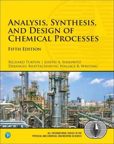
Figure 17.2 shows a flash vessel. For simplicity, the system is considered to be isothermal. The species conservation equation can be written as

Figure 17.2 Schematic of a Flash Vessel

\begin{matrix} \frac{d N_{i}}{dt} = F z_{i} - V y_{i} - L x_{i} \end{matrix} (17.4)

$\begin{matrix} \frac{d N_{i}}{dt} = F z_{i} - V y_{i} - L x_{i} \end{matrix} (17.4)$

where N_i is the molar holdup of species i; F, V, and L are the flowrates of the feed, vapor product, and liquid product, respectively; and z_i, y_i, and x_i are the mole fractions of species i in the feed, vapor product, and liquid product, respectively. Noting that holdup of the species occurs in both liquid and vapor phases, an expression for N_i can be developed:

\begin{matrix} N_{i} = N^{v} y_{i} + N^{l} x_{i} = V^{v} C^{v} y_{i} + V^{l} C^{l} x_{i} = A (H - h) C^{v} y_{i} + Ah C^{l} x_{i} \end{matrix} (17.5)

$\begin{matrix} N_{i} = N^{v} y_{i} + N^{l} x_{i} = V^{v} C^{v} y_{i} + V^{l} C^{l} x_{i} = A (H - h) C^{v} y_{i} + Ah C^{l} x_{i} \end{matrix} (17.5)$

where N^v and N^l are the total molar holdups in the vapor and liquid phases, respectively; V^v and V^l are the volumes of the vapor and liquid phases, respectively; C^v and C^l are the molar densities of the vapor and liquid phases, respectively; A and H are the cross-sectional area and height of the vessel, V-2001, respectively; and h is the height of the liquid at time t inside the vessel. Substituting Equation (17.5) in Equation (17.4) gives

\begin{matrix} A \frac{d [(H - h) C^{v} y_{i} + h C^{l} x_{i}]}{dt} = F z_{i} - V y_{i} - L x_{i} i = 1 \dots n \end{matrix} (17.6)

$\begin{matrix} A \frac{d [(H - h) C^{v} y_{i} + h C^{l} x_{i}]}{dt} = F z_{i} - V y_{i} - L x_{i} i = 1 \dots n \end{matrix} (17.6)$

The phase-equilibrium equations are written as

\begin{matrix} y_{i} = K_{i} x_{i} i = 1 \dots n \end{matrix} (17.7)

$\begin{matrix} y_{i} = K_{i} x_{i} i = 1 \dots n \end{matrix} (17.7)$

The summation equations can be written as

\begin{matrix} \sum_{i = 1}^{n} y_{i} - 1 = 0 \end{matrix} (17.8)

$\begin{matrix} \sum_{i = 1}^{n} y_{i} - 1 = 0 \end{matrix} (17.8)$

\begin{matrix} \sum_{i = 1}^{n} x_{i} - 1 = 0 \end{matrix} (17.9)

$\begin{matrix} \sum_{i = 1}^{n} x_{i} - 1 = 0 \end{matrix} (17.9)$

A suitable thermodynamic model is required for calculating C^v, C^l, and K.

Summing up the total number of equations listed in Equations (17.6) through (17.9) for n species gives a total of 2n + 2 equations. However, the unknown variables are n vapor mole fractions, y_i, n liquid mole fractions, x_i, molar flowrates F, V, and L, vessel pressure P, and the height of the liquid in the vessel, h. Therefore, the total number of unknown variables is 2n + 5. It should be noted that the variables F and h are not calculated in the steady-state simulation of the flash block because F is known, either specified by the user or obtained from the upstream block, and h is not required in the steady-state solution. Therefore, P can be calculated in a steady-state simulation by a user-specified correlation or other detailed momentum balance equation, or it can simply be a constant specified by the user. The dynamic description given previously is underdefined. To make this system square (i.e., the number of equations is equal to the number of unknowns), the flash block, which is a pressure node, must be connected via flow devices as shown in Figure 17.3.

A diagram of a flash vessel connected with flow devices is shown.

Figure 17.3 The Modified Schematic of the Flash Vessel Connected with the Flow Devices

In Figure 17.3, the flow devices are the valves, VLV-1101, VLV-1102, and VLV-1103. Assuming linear characteristics for the valves, the corresponding flow/pressure equations are

\begin{matrix} F = C_{o, 1} V S_{1} \sqrt{\frac{P_{4} - P}{ρ_{F}}} \end{matrix} (17.10)

$\begin{matrix} F = C_{o, 1} V S_{1} \sqrt{\frac{P_{4} - P}{ρ_{F}}} \end{matrix} (17.10)$

\begin{matrix} V = C_{o, 2} V S_{2} \sqrt{\frac{P - P_{5}}{ρ_{V}}} \end{matrix} (17.11)

$\begin{matrix} V = C_{o, 2} V S_{2} \sqrt{\frac{P - P_{5}}{ρ_{V}}} \end{matrix} (17.11)$

\begin{matrix} L = C_{o, 3} V S_{3} \sqrt{\frac{P + ρ_{L} gh - P_{6}}{ρ_{L}}} \end{matrix} (17.12)

$\begin{matrix} L = C_{o, 3} V S_{3} \sqrt{\frac{P + ρ_{L} gh - P_{6}}{ρ_{L}}} \end{matrix} (17.12)$

where F, V, and L are the feed, vapor, and liquid volumetric flowrates entering/leaving V-1101; and C_o_,1, C_o_,2, and C_o_,3 are control-valve flow coefficients for VLV-1101, VLV-1102, and VLV-1103, respectively. It should be noted that in the above formulation there is no pressure drop assumed across V-1101; therefore, the pressures of Streams 1, 2, and 3 (P₁, P₂, and P₃) are related by P = P₁ = P₂ and P₃ = P + ρ_Lgh. The mass density of Streams 1, 2, and 3 is given by ρ_F, ρ_L and ρ_V respectively, and VS₁, VS₂, and VS₃ are the valve-stem positions (expressed as a fraction) of VLV-1101, VLV-1102, and VLV-1103, respectively. To make the system of equations consistent, the pressures at the system boundaries, P₄, P₅, and P₆, are considered constant. The system of equations now becomes well defined. This example shows why the pressure nodes are to be connected to the flow devices to make the system well defined. If a pressure drop in the vessel is considered, then the pressure of Stream 1 is no longer equal to P, the vessel pressure and an additional equation would be required. Similarly, the pressure drop in the piping between the vessel and the valves can be considered but requires additional equations to make the system well defined. For a nonisothermal, flash block model, the temperatures of the streams entering and leaving the flash are additional variables, and the additional equation is the energy conservation equation.

Unsupported Blocks. Certain types of blocks can be adequate for a steady-state simulation and are therefore supported by steady-state simulators, but these blocks may not be appropriate in a dynamic simulation. Such blocks do not usually represent any real unit operation or may be unsupported blocks in a simulator for which the dynamic model is not available in that specific simulation software. For example, a “component separator” block is supported in Aspen Plus, but not in Aspen Plus Dynamics. In a steady-state model, this block can be used to split a feed into two or more products based on user-specified composition(s). While such a composition can be obtained from the experimental or literature data at a given operating condition, it is expected to vary during the transients, and, therefore, such blocks cannot be appropriately represented in a dynamic model. In addition, there may be unsupported blocks, such as the blocks handling solids, for which the dynamic model is not yet available in a simulator software. The simulator manual should be consulted for this information. All unsupported blocks must be replaced by appropriate supported blocks.

17.2.2 Step 2: Equipment Geometry and Size

First-principles models are based on conservation equations. The conservation equations for a dynamic model are written as

\begin{matrix} \begin{matrix} Rate of accumulation = & Rate of inputs + Rate of addition / generation \\ - Rate of outputs - Rate of consumption \end{matrix} \end{matrix} (17.13)

$\begin{matrix} \begin{matrix} Rate of accumulation = & Rate of inputs + Rate of addition / generation \\ - Rate of outputs - Rate of consumption \end{matrix} \end{matrix} (17.13)$

Note that the term on the left-hand side of Equation (17.13) does not appear in a steady-state model. This term is expressed as

\begin{matrix} Rate of accumulation = \frac{d [(holdup volume) (appropriate terms)]}{dt} \end{matrix} (17.14)

$\begin{matrix} Rate of accumulation = \frac{d [(holdup volume) (appropriate terms)]}{dt} \end{matrix} (17.14)$

The “appropriate terms” in Equation (17.14) depend upon the conserved variable. Equation (17.14) shows that the volume information plays a key role in calculating the rate of accumulation or mass or momentum or energy. The equipment should be sized appropriately, mainly based on the steady-state results. Most steady-state process simulators provide sizing routines for the trays and packings in distillation columns. Other equipment can be sized using appropriate software, heuristics, or following this and other books in this area [1–3]. Some useful information about equipment sizing from the perspective of dynamic simulation can be found elsewhere [4] and in Chapters 20 through 23.

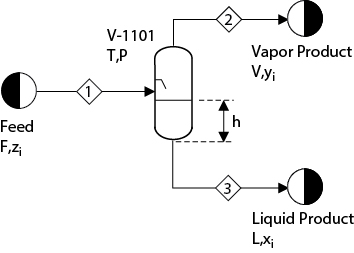
The vessel size, the equipment geometry, and the equipment orientation can have a significant impact on the transient response of certain types of equipment. For example, the orientation of a flash vessel can be horizontal or vertical, as shown in Figure 17.4(a)(b). For a given length L, radius r, and height of liquid h, the holdup volume of the vertical and horizontal vessels is given by (neglecting the volume of the heads)

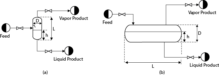
Illustrations of the vertical and horizontal orientations of vessels.

Figure 17.4 Vessels with Different Orientations: (a) Vertical Orientation; (b) Horizontal Orientation

\begin{matrix} V_{vertical} = π r^{2} h \end{matrix} (17.15)

$\begin{matrix} V_{vertical} = π r^{2} h \end{matrix} (17.15)$

\begin{matrix} V_{horizontal} = L [r^{2} {cos}^{- 1} (\frac{r - h}{r}) - (r - h) \sqrt{2 rh - h^{2}}] \end{matrix} (17.16)

$\begin{matrix} V_{horizontal} = L [r^{2} {cos}^{- 1} (\frac{r - h}{r}) - (r - h) \sqrt{2 rh - h^{2}}] \end{matrix} (17.16)$

As shown by Equations (17.15) and (17.16), the holdup volumes for a given height of the liquid, and therefore the transient response, can be considerably different between both types of vessels, even if the inlet and outlet flowrates to both types of vessels are the same. If the holdup volumes are the same in two such vessels, the height can be significantly different, which affects the pressure at the upstream of the discharge liquid control valve at a given vessel pressure.

In addition, the equipment geometry can have an effect on the transient response. For example, if the flash vessel is vertical, as in Figure 17.4(a), and the liquid level at any time is above the vessel tangent line (the hypothetical line that passes through the points of contact between the cylinder and the knuckle portion of the vessel head), the geometry of the vessel head has no effect on the rate of accumulation. However, for a horizontal vessel, the head geometry has an effect (albeit small in most cases) on the transient no matter where the level is being maintained. The geometry can have an effect on the heat loss from a vessel to the environment or on the heat transfer to or from a vessel if a heating/cooling jacket is considered. Two vessels having the same volume and the same wall thickness but different L/D ratios will have different surface areas, which affect their temperature transients. For tray distillation columns, the tray design, such as the diameter, spacing, weir height, downcomer dimension, and type of tray, can have a significant effect on the dynamics of holdup and residence time. Chapter 23 may be consulted for additional details on the design of flash vessels.

17.2.3 Step 3: Additional Dynamic Data/Dynamic Specification

The additional data/dynamic specifications required for transient simulation are equipment specific. In the following discussion, the key dynamic information for common equipment items will be presented. Before the discussion of equipment-specific dynamic data, a discussion that is applicable to most equipment items is presented.

The effect of the ambient conditions, such as the temperature, pressure, and humidity, on the transient response depends on the type of equipment used and the model fidelity. For example, the heat loss to the environment depends upon the ambient temperature. The operation of an air compressor that uses atmospheric air is highly affected by the ambient pressure, temperature, and humidity. In addition, the metal mass of a piece of equipment plays a key role in its temperature transients. The metal mass includes the mass of the entire equipment item including the internals, if any. To clarify further, it can be noted that the accumulation term in the energy conservation equation is written as

\begin{matrix} Rate of accumulation of energy = \frac{dU}{dt} \end{matrix} (17.17)

$\begin{matrix} Rate of accumulation of energy = \frac{dU}{dt} \end{matrix} (17.17)$

where U is the internal energy of the system. Equation (17.17) has been written neglecting the change in kinetic and potential energy. Since

\begin{matrix} H = U + PV \end{matrix} (17.18)

$\begin{matrix} H = U + PV \end{matrix} (17.18)$

where H is the enthalpy, Equation (17.17) can be written as

\begin{matrix} \frac{dU}{dt} = \frac{dH}{dt} - P \frac{dV}{dt} - V \frac{dP}{dt} \end{matrix} (17.19)

$\begin{matrix} \frac{dU}{dt} = \frac{dH}{dt} - P \frac{dV}{dt} - V \frac{dP}{dt} \end{matrix} (17.19)$

The expression for H depends upon the equipment type, the number of phases within the equipment, whether their temperatures are considered to be equal, and other assumptions. Considering the example of the flash block shown in Figure 17.2, H can be calculated by

\begin{matrix} H = N^{v} M^{v} h^{v} + N^{l} M^{l} h^{l} + M_{eq} h_{eq} \end{matrix} (17.20)

$\begin{matrix} H = N^{v} M^{v} h^{v} + N^{l} M^{l} h^{l} + M_{eq} h_{eq} \end{matrix} (17.20)$

In Equation (17.20), M² and M² are the average molecular weights of the vapor and liquid phases, respectively, and h² and h² are the specific enthalpy of the vapor and liquid phases, respectively. Calculation of h² and h² depends on the properties package used in the process simulator. M_eq and h_eq are the metal mass and the specific enthalpy of the metal, respectively. With further simplification, it can be seen that

\begin{matrix} \frac{dH}{dt} = \frac{d (N^{v} M^{v} h^{v})}{dt} + \frac{d (N^{l} M^{l} h^{l})}{dt} + M_{eq} \frac{d (C_{p, eq} T)}{dt} \end{matrix} (17.21)

$\begin{matrix} \frac{dH}{dt} = \frac{d (N^{v} M^{v} h^{v})}{dt} + \frac{d (N^{l} M^{l} h^{l})}{dt} + M_{eq} \frac{d (C_{p, eq} T)}{dt} \end{matrix} (17.21)$

where C_p,eq is the equivalent heat capacity of the metal.

Equation (17.21) shows why the metal mass plays a key role in the temperature transient. This term can be the dominant term during start-up and shutdown of a plant and, therefore, should be considered in the models intended for simulating plant start-up and shutdown.

A representative design of the equipment and the materials of construction is needed to calculate the metal mass. This is usually done in Step 2 as part of the equipment design.

Heat Exchangers. The dynamic models for heat exchangers in process simulators are usually lumped-parameter models. In a lumped-parameter model, the process variables are assumed to vary only with time; therefore, their spatial variation is neglected. However, in a heat exchanger, the temperature of the fluids, and, therefore, the thermodynamic and transport properties, vary with location. Therefore, a rigorous heat-exchanger model should be a distributed-parameter model, where the process variables are considered to vary with space and time. Such models quickly become intractable in dynamic simulations of large process systems and are rarely used. Various simplifications are also made in the lumped-parameter models for easier solution of the equations. These points will be discussed below. In the following discussion, whenever rigorous models are mentioned, it is assumed that these refer to rigorous, lumped-parameter models and not to distributed-parameter models. In process flowsheets, both utility heaters/coolers and process heat exchangers are used.

Utility Heaters/Coolers. For heaters/coolers, where a utility is used for heating/cooling a process stream, a temperature or heat duty is provided in the steady-state model. A simple lumped-parameter, dynamic model of the process side of a utility heater/cooler can be written as

\begin{matrix} \frac{d H^{p}}{dt} = \dot{m} (h_{in}^{p} - h_{out}^{p}) + \dot{Q} \end{matrix} (17.22)

$\begin{matrix} \frac{d H^{p}}{dt} = \dot{m} (h_{in}^{p} - h_{out}^{p}) + \dot{Q} \end{matrix} (17.22)$

where superscript p denotes process stream, and H, h_in, h_out, and ṁ represent enthalpy of process holdup, specific enthalpy of the incoming process stream, specific enthalpy of the exiting process stream, and mass flowrate of the process fluid, respectively. $\dot{Q}$ $\dot{Q}$ is the heat transfer rate. The dynamic heater/cooler models vary depending on how $\dot{Q}$ $\dot{Q}$ is calculated. The appropriate option for calculating $\dot{Q}$ $\dot{Q}$ should depend upon the actual process configuration. Even though the number of possible options varies with the process simulator of choice, four common options will be discussed here. The first option, called the “constant duty” option here, is the simplest case, where the heat duty can be an input variable that can be used as an MV in the dynamic simulation for maintaining the temperature. This option may be used for processes where a heating fluid (such as steam) or a cooling fluid (refrigerant) is being used such that the process temperature is far from the heating/cooling-medium temperature, and it is not expected that the system will ever reach the minimum temperature approach. The underlying assumption of this option is that the dynamics in the heating/cooling medium are very fast and, therefore, can be neglected. With this option, if a temperature controller is not considered and the process-stream flowrate, specific heat, or inlet temperature drastically changes in comparison to its steady-state design conditions, the outlet temperature can be unrealistic and the simulation may fail to converge. In the second option, called the “constant medium temperature” option here, while calculating $\dot{Q}$ $\dot{Q}$ using Equation (17.23), the heating/cooling medium temperature is assumed to remain constant at the inlet temperature as shown in Equation (17.24).

\begin{matrix} \dot{Q} = U_{h} A Δ T_{lm} \end{matrix} (17.23)

$\begin{matrix} \dot{Q} = U_{h} A Δ T_{lm} \end{matrix} (17.23)$

\begin{matrix} Δ T_{lm} = \frac{(T_{in}^{p} - T_{m}) - (T_{out}^{p} - T_{m})}{\ln [(T_{in}^{p} - T_{m}) / (T_{out}^{p} - T_{m})]} \end{matrix} (17.24)

$\begin{matrix} Δ T_{lm} = \frac{(T_{in}^{p} - T_{m}) - (T_{out}^{p} - T_{m})}{\ln [(T_{in}^{p} - T_{m}) / (T_{out}^{p} - T_{m})]} \end{matrix} (17.24)$

In Equation (17.24), T_m, T_in, T_out denote the temperature of the heating/cooling medium, inlet, and outlet process streams, respectively. This option is appropriate when the change in the heating/cooling-medium temperature along the length of the separator/vessel is negligible, and its flowrate is kept constant in the dynamic simulation. The first two options do not take into account the cooling/heating-medium flowrate and the change in the utility temperature due to heat exchange. Therefore, they cannot be used in dynamic simulations where the flowrate of the medium varies (i.e., it is a DV or an MV) and/or the utility flow must be accounted for. Therefore, in the third option, called the “LMTD” option here, the effect of the flowrate of the medium and its temperature change due to heat exchange are considered. Neglecting the temperature dynamics of the medium, in this option, the medium temperature is calculated by (assuming that the specific heat of the medium is constant and there is no phase change of the medium)

\begin{matrix} \dot{Q} = {\dot{m}}_{m} C_{p, m} (T_{m, out} - T_{m, in}) \end{matrix} (17.25)

$\begin{matrix} \dot{Q} = {\dot{m}}_{m} C_{p, m} (T_{m, out} - T_{m, in}) \end{matrix} (17.25)$

where ṁ_m, C_p,m, T_m,out, and T_m,in are the flowrate, specific heat, and inlet and outlet temperatures of the medium, respectively. In this option, the holdup of the medium is not considered. Additional equations should be written if the temperature transients of the metal mass are considered.

If the heat duty is provided by evaporating/condensing a medium, then the option (fourth option) is to model the heat duty by

\begin{matrix} \dot{Q} = {\dot{m}}_{m} λ \end{matrix} (17.26)

$\begin{matrix} \dot{Q} = {\dot{m}}_{m} λ \end{matrix} (17.26)$

where λ is the specific latent heat of the evaporating/condensing medium.

It should be noted that many variations are possible while calculating $\dot{Q}$ $\dot{Q}$ other than those mentioned above. In addition, the equations provided above under each option do not conform to any specific simulator. For the options and the corresponding equations used in a specific simulator platform, the reader should consult the specific user manual.

Example 17.1 demonstrates how the option chosen for a cooler affects its transient response and the final steady-state temperature.

Example 17.1

Steam is being condensed in a surface condenser of a steam turbine under vacuum using cooling water. The flowrate of the steam to the condenser is 50 kmol/h at a temperature and pressure of 55°C and 0.12 bar, respectively. The pressure drop in the condenser is 0.02 bar. At the outlet of the condenser, the steam is completely condensed without any subcooling. Cooling water is available at a temperature and pressure of 25°C and 5 bar, respectively. Design the cooler such that the cooling water temperature at the condenser outlet is 35°C. The maximum allowable pressure drop of the cooling water is 0.5 bar. Develop three dynamic models of this condenser using the “constant duty” option, the “constant medium temperature” option, and the “LMTD” option. Compare the transient response of the process outlet temperature for each of the options when the flowrate of the steam is step decreased to 45.5 kmol/h.

Solution

The problem is set up in Aspen Engineering Suite (AES) using Aspen Plus V9.0, Aspen Plus Dynamics V9.0, and Exchanger Design and Rating (EDR) V9.0. In Aspen Plus, the heater/cooler volume can be provided under “dynamic options.” The volume can be distributed between inlet and outlet volumes. In addition, the quantity of the metal mass can be provided. Considering that the steam is in the shell side, the shell volume and the shell mass are calculated using Aspen EDR. In Aspen EDR, the design objective for optimization is considered to be minimization of cost. The default design options for shell-and-tube heat exchangers in EDR are used. The designed heat exchanger has one shell of diameter 0.337 m, tube OD of 0.019 m, tube ID of 0.015 m, tube length of 2.44 m, 117 tubes, and a shell weight (including the heads) of 392 kg. The material of construction is carbon steel. As mentioned before, the shell- and tube-side volumes can be provided under “dynamic options” in Aspen Plus, with options for providing separate inlet and outlet volumes. In this simulation, the shell-side and tube-side volumes are calculated from the heat-exchanger design mentioned above and then divided into two equal volumes for the inlet and outlet volumes. A similar approach is taken for the metal mass. Three condenser models are considered in Aspen Plus, all with the same steady-state specifications, but the dynamic specifications are as per the problem statement. The converged Aspen Plus simulation is exported to Aspen Plus Dynamics, and after running the dynamic simulation for about 0.08 h, the flowrate of steam is decreased from 50 kmol/h to 45.5 kmol/h. No controller is implemented; that is, neither the heat duty, the medium temperature, nor the medium flowrate is changed. The transient response of the process stream at the outlet of the condensers is shown in Figure E17.1. The temperature at the outlet of the condenser with the “constant duty” option reaches a negative value. Even with this severe temperature cross, the simulation continues without any warning. When the steam flowrate is decreased, it would be expected that the cooling water outlet temperature would decrease. Thus, the condenser with the “LMTD” option shows a lower condenser outlet temperature than the condenser with “constant medium temperature” option, that is, a few degrees of subcooling. The temperature response of the exchanger with the “LMTD” option is as expected. This example demonstrates that the user needs to be careful about the choice of the heat-exchanger blocks to avoid unrealistic results from a dynamic simulation.

A graph showing the transient response of the condenser outlet temperature with different options.

The horizontal axis is labeled Time (hours), ranging from 0 to 4.0, in increments of 0.5. The vertical axis is labeled Temperature (degrees Celsius), ranging from negative 20 to 50, in increments of 10. A line labeled Cooling Water Inlet Temperature runs parallel to the horizontal axis from the point (0, 25). The three line graphs described below all begin at (0, 45), continue as a straight line to (1.5, 45), then curve down, and proceeds as a straight line parallel to the horizontal axis. The line representing T subscript (out, constant duty), curves steeply down to the point (1.75, negative 10), and proceeds at a straight line to (3.75, negative 10). The line pertaining to T subscript (out, constant medium temperature), curves slightly down to (1.75, 40), and proceeds as a straight line up to (3.75, 40). The line denoting T subscript (out, LMTD), steps down to (1.75, 42), and continues as a straight line up to (3.75, 42).

Figure E17.1 Transient Response of the Condenser Outlet Temperature with “Constant Duty” Option, “Constant Medium Temperature” Option, and “LMTD” Option

Process Heat Exchanger. For simulating process heat exchangers, two options will be considered. In the first, which will be called the “simple” option, the process heat exchangers will be simulated simply by combining a heater with a cooler and equating their heat duties, as shown in Figure 17.5(a). This option is widely used in steady-state simulation. In a steady-state simulation, the outlet temperature of E-1101A/E-1101B or its heat duty can be specified, ensuring that the minimum temperature approach is not violated. However, if the flowrates and/or the temperatures of the hot and cold streams vary in the dynamic simulation, there can be a temperature cross. Even though this is physically impossible, the simulation may not report this error and continue. This can result in completely unrealistic transient response and steady-state results as seen in Example E17.2. The second option is to consider a heat exchanger as shown in Figure 17.5(b). This will be called a “rigorous exchanger,” in the sense that this option is a rigorous lumped-heat-exchanger model with appropriate methods for calculating heat transfer coefficients.

Illustrations of the simple and rigorous configurations of process heat exchangers.

Figure a shows a simple configuration of process heat exchangers. The input stream 1 is labeled Cold Stream In, is sent to E-1101A, which is a part of the heat exchanger, that sends an output stream 2 labeled Cold Stream Out. The input stream 3 is labeled Hot Stream In, is sent to E-1101B, which is the other part of the heat exchanger, that sends an output stream 4 labeled Cold Stream Out. E-1101B points to E-1101A with an arrow labeled Q. Figure b shows a rigorous configuration of process heat exchangers. Here, the input streams 1 and 3 enter the single heat exchanger E-1101, through its left and bottom-left, respectively. Similarly, the output streams 4 and 2 leave E-1101 through its right and top-right, respectively. The streams are labeled as in figure a. The temperatures of the streams are as follows in both figures: T subscript (c, in), T subscript (c, out), T subscript (h, in), and T subscript (h, out). The mass flow rates of the input streams are m dot subscript c and m dot subscript h, respectively.

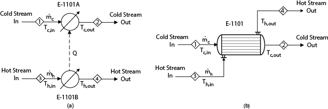
Figure 17.5 Configurations of Process Heat Exchangers: (a) Simple Configuration; (b) Rigorous Configuration

A simple model of a rigorous heat exchanger can be written as

\begin{matrix} \frac{d H^{c}}{dt} = {\dot{m}}_{c} (h_{in}^{c} - h_{out}^{c}) + \dot{Q} \end{matrix} (17.27)

$\begin{matrix} \frac{d H^{c}}{dt} = {\dot{m}}_{c} (h_{in}^{c} - h_{out}^{c}) + \dot{Q} \end{matrix} (17.27)$

\begin{matrix} \frac{d H^{h}}{dt} = {\dot{m}}_{h} (h_{in}^{h} - h_{out}^{h}) + \dot{Q} \end{matrix} (17.28)

$\begin{matrix} \frac{d H^{h}}{dt} = {\dot{m}}_{h} (h_{in}^{h} - h_{out}^{h}) + \dot{Q} \end{matrix} (17.28)$

\begin{matrix} \dot{Q} = UA Δ T_{lm} \end{matrix} (17.29)

$\begin{matrix} \dot{Q} = UA Δ T_{lm} \end{matrix} (17.29)$

In Equations (17.27) and (17.28), superscripts c and h denote cold and hot streams, respectively. Other variables have connotaions similar to Equation (17.22). Additional equations are required if the effect of the metal mass is considered. As mentioned before, such considerations play a key role in the transient response of the models intended for simulating plant start-up/shutdown. In addition, based on the expected skin temperature of a heat exchanger, it may be important to consider the heat loss to the environment.

Example 17.2 shows that a simple process heat exchanger can give unrealistic results under certain process conditions. In this and other examples in this chapter, the specifications shown in the flowsheet are the steady-state values.

Example 17.2

Develop two dynamic models of the process heat exchanger shown in Figures E17.2(a)(a) and E17.2(a)(b), one with the simple option and another with the rigorous option. In this process heat exchanger, at the design condition, Stream 1, a mixture of methane and ethane, is to be heated to 200°C by a hot stream of ethane. Initially the process is at steady state. Then the flowrate of Stream 1 is decreased by a step change to 45 kmol/h. Show the transient response of the outlet temperatures of the hot and cold streams from both the heat-exchanger models. Assume heat loss to the environment to be negligible.

Figures of the simple and rigorous configurations of process heat exchangers.

Figure "a" shows a simple configuration of process heat exchangers. The input stream 1 is labeled Cold Stream In, is sent to E-1101A, which is a part of the heat exchanger, that sends an output stream 2 labeled Cold Stream Out. The input stream 3 is labeled Hot Stream In, is sent to E-1101B, which is the other part of the heat exchanger, that sends an output stream 4 labeled Cold Stream Out. E-1101B points to E-1101A with an arrow labeled Q. Figure b shows a rigorous configuration of process heat exchangers. Here, the input streams 1 and 3 enter the single heat exchanger E-1101, through its left and bottom-left, respectively. Similarly, the output streams 4 and 2 leave E-1101 through its right and top-right, respectively. The streams are labeled as in figure a. The parameters pertaining to Cold Gas In are: 100 kilomoles per hour, 50 degrees Celsius, P equals 5 bar, y subscript methane equals 0.8, and y subscript ethane equals 0.2. The temperature of Cold Gas Out is given to be 200 degrees Celsius. The parameters pertaining to Hot Gas In are: 50 kilomoles per hour, 300 degrees Celsius, P equals 3 bar, and y subscript ethane equals 1.0. The temperature of Hot Gas Out, T subscript (h, out) is asked to be calculated.

Figure E17.2(a) (a) Simple Configuration of a Heat Exchanger; (b) Rigorous Configuration of a Heat Exchanger

The horizontal axis is labeled Time (hours), ranging from 0 to 0.40, in increments of 0.05. The vertical axis is labeled Temperature (degrees Celsius), ranging from negative 100 to 400, in increments of 100. A line labeled Inlet Temperature of the Hot Stream runs parallel to the horizontal axis from the point (0, 300). The line representing T subscript (c, out, sim), begins at (0, 200), continues as a straight line to (0.075, 200), rises gradually to (0.15, 350), where it turns right to continue as a straight line parallel to the horizontal axis up to (0.40, 350). The line pertaining to T (h, out, sim) is a line running parallel to the horizontal from (0, 120). The line pertaining to T subscript (c, out, rig), also begins at (0, 200), and continues as a straight line to (0.075, 200). It then rises instantly and turns right at (0.15, 275), and proceeds as a straight line to (0.40, 275). The line denoting T subscript (h, out, rig), begins at (0,120), continues as a straight line up to (0.075, 120), rises to (0.15, 175), where it turns right and continues as a straight line to (0.40, 180). All coordinate plots are approximate.

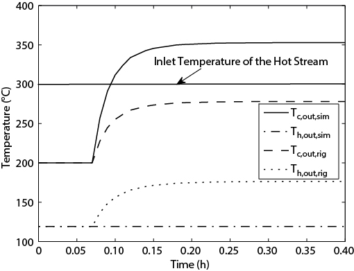
Figure E17.2(b) Transient Response of the Hot and Cold Stream Temperatures for the Simple Heat−Exchanger Configuration and the Rigorous Heat−Exchanger Configuration

Solution

The problem is set up in Aspen Engineering Suite (AES) using Aspen Plus V9.0, Aspen Plus Dynamics V9.0, and Exchanger Design and Rating (EDR) V9.0. In Aspen Plus, the shell- and tube-side volumes of both heat-exchanger models are provided. The volumes are equally distributed between the inlet and outlet volumes. In addition, the quantity of metal mass is provided. For calculating the shell-side and tube-side volumes and the metal mass, Aspen Exchanger Design and Rating V9.0 is used. In this design of a floating-head, shell-and-tube heat exchanger, the hot fluid is located on the shell side. Predictive SRK (PSRK in Aspen Properties) EOS is used for designing the exchanger in EDR and for simulating it in Aspen Plus and Aspen Plus Dynamics. The design objective for the heat-exchanger design is to minimize the cost. The default design options for shell-and-tube heat exchangers in EDR are used. The designed heat exchanger has one shell of diameter 0.205 m, a tube OD of 0.019 m, a tube ID of 0.015 m, a tube length of 4.877 m, 40 tubes, a shell weight (including the heads) of 356 kg, and a tube-bundle weight of 205 kg. The material of construction for both the shell and tubes is carbon steel. For the simple heat exchanger, the pressure drops on both the shell and tube sides are assumed to be 0.1 psi. For the rigorous heat exchanger, the EDR file is inserted in the heat-exchanger specification sheet. The converged Aspen Plus simulation is then exported to Aspen Plus Dynamics, and after running the dynamic simulation for about 0.08 h, the flowrate of Stream 1 is decreased from 100 kmol/h to 45 kmol/h. The transient response of the hot and cold streams at the outlet of the heat exchangers is shown in Figure E17.2(b). The hot stream temperature in the simple configuration does not change at all, since the heat-exchanger duty remains the same and the inlet condition of the hot stream does not change. There is a temperature cross in the cold stream outlet temperature, because it exceeds 300°C, the inlet temperature of the hot stream. However, the simulation continues without any warning. The temperature response of the rigorous exchanger is as expected. It should be noted that in Aspen Plus Dynamics, the response of the simple exchanger can be made similar to that of the rigorous exchanger by writing “scripts.”

Flash Separators and Storage Vessels. Equations (17.6) through (17.9) describe the dynamic model of a flash vessel. For a storage vessel, only a single phase is considered; thus, Equations (17.6) through (17.9) can be modified accordingly. As mentioned previously, the geometry/size information should be provided for the flash separators and storage vessel. In the case of a nonisothermal model, an energy balance equation is also needed. The energy balance equation is written as

\begin{matrix} \frac{dU}{dt} = F h_{in} - V h^{v} - L h^{l} + {\dot{Q}}_{in} - {\dot{Q}}_{loss} \end{matrix} (17.30)

$\begin{matrix} \frac{dU}{dt} = F h_{in} - V h^{v} - L h^{l} + {\dot{Q}}_{in} - {\dot{Q}}_{loss} \end{matrix} (17.30)$

where h_in, h^v, and h^l are the molar enthalpies of the feed stream, vapor outlet, and liquid outlet, respectively. ${\dot{Q}}_{in}$ ${\dot{Q}}_{in}$ is the rate of heat transfer to the vessel and is considered to be nonzero for a vessel with a heating or cooling jacket. ${\dot{Q}}_{loss}$ ${\dot{Q}}_{loss}$ is the rate of heat loss to the environment and can be considered to be zero for a well-insulated vessel and/or when the vessel temperature is close to the temperature of the environment. For the left-hand term of Equation (17.30), appropriate forms of Equations (17.19) and (17.21) are used. For calculating ${\dot{Q}}_{in}$ ${\dot{Q}}_{in}$ in the dynamic simulation, the options are similar to what has been discussed in the section on utility heaters/coolers. Any of the four options discussed there can be used with the most appropriate option chosen for the situation under consideration. The heat transfer option, whenever applicable, plays a key role in the transient response of the temperature. Example 17.3 shows how the heat transfer option affects not only the temperature of the system but also other state variables.

Example 17.3

Figure E17.3(a) shows the schematic of a jacketed flash vessel in which a mixture of CO₂ and methanol is being separated. The inlet temperature of the heating medium stream is 90°C and its specific heat is similar to that of water. There is no phase change of the heating medium in the jacket. Compare the transient response of the flash vessel outlet temperature and its level for the “constant duty” and “LMTD” options when the inlet feed flowrate is reduced to 10 kmol/h. Assume no change in the inlet temperature and flowrate of the heating medium. The vessel is well insulated; that is, heat loss to the environment may be assumed to be negligible.

A diagram shows the configuration of the jacketed flash vessel for separating carbon-dioxide and methanol.

Stream 1 contains an input feed at 30 degrees Celsius, 5 bars of pressure, 100 kilomoles per hour, y subscript methanol equals 0.9, and y subscript carbon-dioxide equals 0.1. Stream 1 enters FC-1101, which is connected to C V - 1101 directly and through an FC unit. C V - 1101 sends stream 2 to the flash vessel, along with an input Heating Fluid. The flash vessel has a layer, that forms the jacket, coating its bottom half. The vessel is labeled V-1101, has a temperature of 70 degrees Celsius, and P equals 3.0 bar. Heating Fluid is sent out from the vessel through its bottom. Streams 3 and 5 also leave the vessel. Stream 3 is connected to C V - 1102, both directly and through a PC unit. Stream 4 from C V - 1102 produces a Vapor Product. Stream 5 from the vessel is sent to C V - 1103, which is connected back to the vessel through an LC unit. Stream 6 from C V - 1103 contains a Liquid Product. All C V valves have delta P equivalent to 1 bar.

Figure E17.3(a) Configuration of the Jacketed Flash Vessel for Separating CO₂ and Methanol

Solution

The problem is set up in Aspen Engineering Suite (AES) using Aspen Plus V9.0 and Aspen Plus Dynamics V9.0. The Aspen Plus V9.0 simulation is developed by modifying one of the examples for methanol absorbers available in the example flowsheet under Program FilesAspenTechAspen Plus V9.0GUIExamplesPhysical Solvents. For users simulating it in other platforms, it should be noted that the perturbed-chain statistical associating fluid theory (PC-SAFT) EOS is used. In this model, the thermophysical property models have been validated against DIPPR correlations for species vapor pressure and liquid density and against literature data for liquid heat capacity, heat of vaporization, and VLE. The vessel size is calculated considering both liquid holdup and vapor velocity following the heuristics laid out in Table 11.6. Holdup time is considered to be 5 min for the half-full flash vessel. For calculating the gas velocity, the flash vessel is considered to have a mesh demister. It is assumed that L/D = 3. The values of length and diameter are found to be L = 1.92 m and D = 0.64 m. The thickness of the wall is found using carbon steel as the material of construction and by applying the following equation:

t = \frac{PD}{2 SE - 1.2 P} + CA

$t = \frac{PD}{2 SE - 1.2 P} + CA$

where P is the design pressure of the vessel (in bar), D is the diameter of the vessel (m), S is the maximum allowable stress (940 bar for carbon steel), E = 0.9, and CA = corrosion allowance (assumed to be 0.00315 m here). Accordingly, the metal mass of the vessel is calculated. Two models of the flash vessel, one with the “constant duty” option and the other with the “LMTD” option, are set up in Aspen Plus. The simulation is exported to Aspen Plus Dynamics as a pressure-driven simulation. The pressure and the level of the vessel are maintained by PI controllers. The feed flow is decreased to 10 kmol/h. The corresponding transient response of the temperature is shown in Figure E17.3(b)(a). The temperature of the flash vessel with the “LMTD” option does not change appreciably. The initial increase in the temperature of the flash vessel with the “constant heat duty” option is slightly higher than the heat exchanger with the “LMTD” option. However, it is seen in Figure E17.3(b)(b) that the level in the vessel with the “constant duty” option starts decreasing even with the liquid outlet valve completely closed. This is because the rate of vapor flow out is larger than the feed flowrate. Eventually, as the vessel becomes completely empty, the temperature steeply increases, as seen in Figure E17.3(b)(a). Note that the level of the flash vessel using the “LMTD” option is maintained at near its steady-state value after some small transient due to the steep change in feed flow. The reader is encouraged to verify that as the feed valve is completely closed, the temperature of the flash vessel with the “constant duty” option steeply increases to the maximum temperature allowed by the simulator (which is 1995°C in Aspen Plus Dynamics, by default). This example demonstrates that it is important to model the heat transfer option appropriately for jacketed flash vessels to obtain a representative transient response.

Two graphs showing the temperature transient and level of the flash vessel with respect to the transient response of the jacketed flash vessels.

Graph "a" has the horizontal axis labeled Time (hours), ranging from 0 to 6, in unit increments, and the vertical axis labeled Temperature (degrees Celsius), ranging from 0 to 400, in increments of 100. The T subscript (out, constant duty) begins at (0, 80), and continues as a straight line to (1.2, 80), where it rises slightly and proceeds as a straight line up to (3, 100). It rises steeply from here and turns right at (3.2, 300) and continues as a straight line to (5.7, 300). The T subscript (out, LMTD) curve runs almost as a straight line from (0, 80), with a small rise at (1.2, 80). From here it continues as a straight line to (5.7, 100). Graph b has the horizontal axis labeled Time (hours), ranging from 0 to 6, in unit increments, and the vertical axis labeled Level (percentage), ranging from 0 to 60, in increments of 20. The Level subscript (constant duty) curve begins at (0, 70), runs as a straight line to (1.2, 70), where it dips slightly and again proceeds as a slightly rising curve that ends at (5.7, 69). The Level subscript LMTD curve also begins at (0, 70), and runs as a straight line to (1.2, 70). From here is slopes gradually down to the point (2.9, 0). All coordinate plots are approximate.

Figure E17.3(b) Transient Response of the Jacketed Flash Vessels with “Constant Duty” Option and “LMTD” Option: (a) Temperature Transient; (b) Level of the Flash Vessel

Reactors. A number of excellent references discuss dynamic models for nonisothermal CSTR and PFR reactors [5, 6]. Interested readers should review the discussions provided in these books. In a process simulator environment, the user needs to provide the reactor orientation (note that this option matters only when a level is maintained or if the effect of gravity is considered for a liquid-phase reactor) and the reactor size. The reactor size (and therefore the residence time) not only affects the steady-state results but also has a significant effect on the transient response of the product composition and temperature. For dynamic simulation of jacketed reactors, the heat transfer options are similar to those discussed previously for utility heaters/coolers. The heat transfer option can strongly affect the transient response of the reactor. For packed-bed reactors, the catalyst temperature and its dynamics can be different from those of the process stream, especially when the heat transfer coefficient is low. To model such reactors, separate energy conservation equations for the process stream and the catalyst are considered in a process simulator. The model equations for a dynamic PFR consist of partial differential equations (PDEs). As the process simulators usually consider a one-dimensional model of a PFR, the steady-state model can be solved by an efficient ordinary differential equation (ODE) solver. For dynamic simulation of PFRs, two common approaches are to use the method of lines or to approximate the PFR as series of CSTRs.

Method of Lines. In this method, the PDEs are discretized in the spatial dimension, leaving the time variable continuous, generating a system of ODEs. Coupled with the algebraic equations, this generates a system of differential algebraic equations (DAEs). The spatial discretization can be performed by several methods, such as finite-difference methods (backward or central finite difference), orthogonal polynomials (collocation methods), and others. The dynamic simulation can be initialized based on the steady-state results or by a consistent set of initial conditions. However, there can be large errors (which may eventually lead to convergence failure) due to an insufficient number of grid points if there is a large change in the species concentration or temperature. If the number of grid points increases, so does the number of equations. Therefore, the grid size is specified by evaluating the trade-off between accuracy and computation expense. A reasonable grid size for a particular system is often established by a grid sensitivity study.

Series of CSTRs. A PFR can be replaced by a series of CSTRs. In this technique, the state variables can be initialized by using the steady-state results and/or by a consistent set of initial conditions. Similar to the method of lines, the suitable number of CSTRs to replace a single PFR depends upon the system of interest and has to be determined on a case-by-case basis.

Distillation Columns. A number of excellent books are available that discuss the dynamic models and control of distillation columns [7–9]. The condenser of a distillation column is a special type of cooler in which phase change takes place. Therefore, the previous heat transfer options for utility heaters/coolers are applicable. The reflux drum in a distillation column with a partial condenser is similar to a flash vessel, and the discussions provided before are also applicable. The discussion of utility heaters is applicable to kettle- or thermosiphon-type reboilers. In the case of forced-circulation reboilers or fired heaters used as reboilers, pumps are usually used. Therefore, additional equations/unit operations will be required to capture the flow dynamics along with the appropriate heat transfer option. In the case of fired heaters, especially when they are large, a simple heater model is not representative. In large fired heaters, both radiative and convective heat transfer usually play a key role based on the spatial location. In addition, the dynamics of the fuel-oil/fuel-gas stream and the oxidant stream may have a large impact on the dynamics of the process streams. Therefore, appropriate process models should be chosen for these unit operations. The column sump and reflux drum volumes should be calculated mainly based on holdup requirements. For tray columns, the tray hydraulics should also be considered. The dynamic model of a tray can be developed by suitably modifying the equations provided earlier for a flash vessel. Therefore, the liquid and vapor holdup on a tray and the pressure drop (if important) should be modeled precisely. For these calculations, the tray type, spacing, configuration (single/double pass, etc.), the tower diameter, the weir height, the open area, downcomer details, and other characteristic parameters based on a type of tray should be specified. For packed columns, the packing type and packing void fraction, specific surface area, height of packing in a section, packing diameter, and other characteristic parameters based on packing type should be specified. Most steady-state process simulators offer sizing routines, and, therefore, these can be used to generate this information. In addition, the metal mass of the reflux vessel, the sump, trays/packing, and the column shell may be important, especially when a large variation in operating temperature is expected or for dynamic models intended for studying start-up/shutdown. In addition, heat loss to the environment can be modeled.

17.3 Dynamic Simulation Solution Methods

A dynamic model involves the solution of a system of DAEs. The differential equations relate the state variables to other state variables and the manipulated variables. The algebraic equations relate the output variables to the state variables and represent the constitutive relations, properties calculations, and any other closure equations. In addition, the algebraic equations relate the output variables to the state variables. Mathematically,

\begin{matrix} \frac{d x}{dt} = f (x, y, u, d, θ) \end{matrix} (17.31)

$\begin{matrix} \frac{d x}{dt} = f (x, y, u, d, θ) \end{matrix} (17.31)$

\begin{matrix} h (x, θ, y) = 0 \end{matrix} (17.32)

$\begin{matrix} h (x, θ, y) = 0 \end{matrix} (17.32)$

where x, u, d, θ, and y denote state variables, manipulated inputs, disturbance inputs, parameter vector, and algebraic variables, respectively.

The index of a DAE system is defined as the minimum number of times the function h(x, θ, y) must be differentiated to result in a DAE system. For problems that are of index higher than one, $\frac{∂h}{∂y}$ $\frac{∂h}{∂y}$ is singular, and consistent initial conditions must be specified. Most commercial process simulators handle only index-one problems, and, therefore, the discussion that follows pertains only to these types of problems. It should be noted that the stability of any numerical method can be markedly different for the case of higher-index problems, and certain sections of the following discussion are not applicable to problems of higher index. Solving a dynamic simulation involves two steps, namely, initialization and the solution of the DAE system. In the following paragraphs, these steps will be discussed in detail.

17.3.1 Initialization

Process simulators solve first-order ODEs as shown in Equation (17.31). In the initialization step, a consistent set of initial values is calculated by using Equations (17.31) and (17.32). If there are s state variables and w algebraic variables, then a total of s + w equations is available. However, in the initialization steps, the unknowns are s number of x(0), s number of $\frac{dx}{dt} |_{t = 0}$ $\frac{dx}{dt} |_{t = 0}$ , and w number of y(0). Therefore, s number of variables among 2s unknown state variables and their derivatives should be specified. The variables that should be specified depend upon the problem being solved. When the initial state is steady state, then $\frac{d x}{dt} |_{t = 0} = 0$ $\frac{d x}{dt} |_{t = 0} = 0$ . However, if the initial state is a cold start-up or shutdown of the system, or if the system is not at steady state, all or some of the initial values of x(0) can be specified. Additionally, some $\frac{d x}{dt} |_{t = 0}$ $\frac{d x}{dt} |_{t = 0}$ values and/or y(0) values can be specified, if necessary, for making the system square, but such specifications must ensure that they are consistent, that is, that they satisfy Equations (17.31) and (17.32).

17.3.2 Solution of the DAE System

As seen previously, it may be possible to convert the system of DAEs shown in Equation (17.31) to a system of ODEs by differentiating the algebraic equations and manipulating them. However, this procedure can be very tedious for many systems and is not always guaranteed to produce a system of ODEs in explicit form. Therefore, the popular approach is to carry out numerical integration of the differential equations in Equation (17.31) and then solve them along with the algebraic equations. Therefore, a linear/nonlinear algebraic system of equations is finally solved. However, the process dynamic simulators vary based on how the DAEs are solved. These are broadly divided into two methods, namely, modular and simultaneous.

Modular. The modular method is similar to the sequential modular (SM) method discussed in Chapter 16 for steady-state simulation. The idea is to solve the dynamic model of individual equipment separately and then iterate until a converged solution is reached. However, as discussed in Section 17.2.1, the flow into and out of a unit operation depends upon the upstream and downstream pressures of the corresponding blocks in a dynamic simulation. This necessitates an iterative approach even in the absence of a recycle. In the presence of recycle, tear streams are generated similar to the SM method. However, the initial guess for temporal variations of the tear stream is needed. This usually makes it much more computationally expensive, especially for large simulations and if a large number of recycles are present. The advantages are in using an efficient solution approach for specific unit operations instead of using a general-purpose equation solver and easier troubleshooting in the case of convergence failure.

Simultaneous. In this method, all the equations for all the blocks are collected together and solved simultaneously. The simultaneous method again can take two different approaches. In one approach, a separate pressure-flow solver is used to solve only the pressure-flow network equations, while other equations can be solved at a different time interval (frequency). This approach has two advantages. First, an efficient solution approach for specific unit operations can be used. Second, time-consuming calculations such as flash calculations can be carried out at different frequencies. Another approach is to solve all the equations simultaneously, including the pressure-flow equations. This approach guarantees stability and accuracy of solution as long as an appropriate solver is chosen. These concepts will be made clear in the following discussions.

For solving the differential equations, an efficient integrator algorithm is required. As the integrator algorithm generates a set of linear/nonlinear equations, an efficient algebraic equation solver is also required for solving the coupled equations. A brief account of the integrator and linear/nonlinear algebraic equation solver algorithms will now be provided.

Dynamic Simulation Integrator Algorithms. Before further discussion of integrator algorithms, the definition of a stiff problem will be provided. Considering Equation (17.31), if $J = \frac{∂f}{∂x}$ $J = \frac{∂f}{∂x}$ and the matrix J has eigenvalues λ_i for which max|λ_i|≫min|λ_i|, then the system is called stiff. Stiff problems can be difficult to solve and need special consideration when applying numerical methods. These points are discussed below.

Various numerical integration methods are usually taught as part of a numerical methods course. Therefore, only the salient points that are important from the point of view of dynamic simulation of a process model will be covered here.

Explicit Methods. In explicit methods, state variables at any time instant n + 1 are explicitly written in terms of the variables at the previous instant, that is, at time n. For Equation (17.31), this takes the form

\begin{matrix} x_{n + 1} = g (x_{n}, y_{n}, u_{n}, d_{n}, θ) \end{matrix} (17.33)

$\begin{matrix} x_{n + 1} = g (x_{n}, y_{n}, u_{n}, d_{n}, θ) \end{matrix} (17.33)$

This approach can be very advantageous for a system of ODEs, since the solution of a system of nonlinear equations is avoided. However, in the case of a DAE system, which usually is the case for a process simulation, a nonlinear system of equations still needs to be solved because of the coupled algebraic equations. The explicit Euler method is available in most dynamic simulators and will be discussed below.

Explicit Euler Method. This is probably the simplest first-order, explicit method based on a forward difference approximation of the derivative. Considering Equation (17.31), the numerical integration is written as

\begin{matrix} x_{n + 1} = x_{n} + Δ t_{n} f (x_{n}, y_{n}, u_{n}, d_{n}, θ) \end{matrix} (17.34)

$\begin{matrix} x_{n + 1} = x_{n} + Δ t_{n} f (x_{n}, y_{n}, u_{n}, d_{n}, θ) \end{matrix} (17.34)$

This method is stable for a restrictive time step, beyond which it may be unstable; that is, x will eventually grow without limits and the integrator will fail to converge. The stiffer the system is, the smaller the time step must be to obtain a stable solution. On the other hand, the simulation should be run until the process with the smallest time constant has reached its new steady state. In addition, a much smaller time step than is required for stability will make the approach computationally inefficient. This makes the Euler method difficult to use for large process simulations containing thousands of equations and where the time scales of different processes are widely different.

A few other explicit methods will also be discussed under “Multistep Methods.”

Implicit Methods. In implicit methods, irrespective of whether an ODE or a DAE system is being solved, a system of algebraic equations needs to be solved. The biggest advantage of any implicit method is that it is stable for large step sizes, and some implicit algorithms are stable for any step size. However, a larger step size can cause errors in solution or convergence failure. Therefore, it makes sense to modify the step size adaptively: using a smaller step size when there is a significant change, and using a larger step size otherwise.

Implicit Euler Method. This is probably the simplest first-order implicit method based on a backward difference approximation of the derivative. Considering Equation (17.31), the numerical integration is written as

\begin{matrix} x_{n + 1} = x_{n} + Δ t_{n} f (x_{n + 1}, y_{n + 1}, u_{n + 1}, d_{n + 1}, θ) \end{matrix} (17.35)

$\begin{matrix} x_{n + 1} = x_{n} + Δ t_{n} f (x_{n + 1}, y_{n + 1}, u_{n + 1}, d_{n + 1}, θ) \end{matrix} (17.35)$

Trapezoidal Method. This is a very popular second-order, single-step method.

\begin{matrix} x_{n + 1} = x_{n} + \frac{Δ t_{n}}{2} (f (x_{n + 1}, y_{n + 1}, u_{n + 1}, d_{n + 1}, θ) + f (x_{n}, y_{n}, u_{n}, d_{n}, θ)) \end{matrix} (17.36)

$\begin{matrix} x_{n + 1} = x_{n} + \frac{Δ t_{n}}{2} (f (x_{n + 1}, y_{n + 1}, u_{n + 1}, d_{n + 1}, θ) + f (x_{n}, y_{n}, u_{n}, d_{n}, θ)) \end{matrix} (17.36)$

Multistep Methods. Multistep methods can be explicit or implicit. This family of methods is widely applicable for different types of process models. The generic formulation for the methods in this class is given by

\begin{matrix} x_{n + 1} = \sum_{i = 0}^{q} a_{i} x_{n - i} + Δ t_{n} \sum_{j = 0}^{q + 1} b_{i} f (x_{n + 1 - j}, y_{n + 1 - j}, u_{n + 1 - j}, d_{n + 1 - j}, θ) \end{matrix} (17.37)

$\begin{matrix} x_{n + 1} = \sum_{i = 0}^{q} a_{i} x_{n - i} + Δ t_{n} \sum_{j = 0}^{q + 1} b_{i} f (x_{n + 1 - j}, y_{n + 1 - j}, u_{n + 1 - j}, d_{n + 1 - j}, θ) \end{matrix} (17.37)$

Note that if b₀ is set to zero, this becomes an explicit method. Any multistep method can be used for different polynomial orders. Different multistep methods differ in how the index q varies based on the polynomial order and which coefficients are set to zero. Under this category, one of the most popular methods is Gear’s method. In Gear’s method,

\begin{matrix} q = k - 1 \\ b_{1} = b_{2} = \dots . . = b_{k} = 0 \end{matrix} (17.38)

$\begin{matrix} q = k - 1 \\ b_{1} = b_{2} = \dots . . = b_{k} = 0 \end{matrix} (17.38)$

A fourth-order Gear’s formula is given by

\begin{matrix} x_{n + 1} = a_{0} x_{n} + a_{1} x_{n - 1} + a_{2} x_{n - 2} + a_{3} x_{n - 3} + Δ t_{n} b_{0} f (x_{n + 1}, y_{n + 1}, u_{n + 1}, d_{n + 1}, θ) \end{matrix} (17.39)

$\begin{matrix} x_{n + 1} = a_{0} x_{n} + a_{1} x_{n - 1} + a_{2} x_{n - 2} + a_{3} x_{n - 3} + Δ t_{n} b_{0} f (x_{n + 1}, y_{n + 1}, u_{n + 1}, d_{n + 1}, θ) \end{matrix} (17.39)$

where a_{0} = \frac{48}{25}, a_{1} = - \frac{36}{25}, a_{2} = \frac{16}{25}, a_{3} = - \frac{3}{25}, b_{0} = \frac{12}{25}

$where a_{0} = \frac{48}{25}, a_{1} = - \frac{36}{25}, a_{2} = \frac{16}{25}, a_{3} = - \frac{3}{25}, b_{0} = \frac{12}{25}$

Two other methods in this category are also popular. These are the Adams-Bashford and the Adams-Moulton methods. The Adams-Bashford method is explicit and the Adams-Moulton method is implicit.

If more points are used in a time interval, that leads to the popular Runge-Kutta family of methods. The Runge-Kutta family of methods can be explicit or implicit. An sth-order explicit Runge-Kutta method for a DAE system, such as Equations (17.31) and (17.32), is given by

\begin{matrix} \begin{array}{l} x_{n + 1} = x_{n} + Δ t_{n} \sum_{i = 1}^{s} b_{i} f (X_{n, i}, Y_{n, i}, U_{n, i}, D_{n, i}, θ) \\ X_{n, i} = x_{n} + Δ t_{n} \sum_{j = 1}^{s} a_{ij} f (X_{n, j}, Y_{n, j}, U_{n, j}, D_{n, j}, θ) \\ h (X_{n, i}, Y_{n, i}, U_{n, i}, D_{n, i}, θ) = 0, i = 1 . . s \end{array} \end{matrix} (17.40)

$\begin{matrix} \begin{array}{l} x_{n + 1} = x_{n} + Δ t_{n} \sum_{i = 1}^{s} b_{i} f (X_{n, i}, Y_{n, i}, U_{n, i}, D_{n, i}, θ) \\ X_{n, i} = x_{n} + Δ t_{n} \sum_{j = 1}^{s} a_{ij} f (X_{n, j}, Y_{n, j}, U_{n, j}, D_{n, j}, θ) \\ h (X_{n, i}, Y_{n, i}, U_{n, i}, D_{n, i}, θ) = 0, i = 1 . . s \end{array} \end{matrix} (17.40)$

A very popular method in this family is the fourth-order, explicit Runge-Kutta method. Implicit Runge-Kutta methods are also known as the Gauss-Legendre method. They are computationally expensive but have very good stability properties.

Predictor-Corrector Methods. The implicit methods can be used effectively to solve stiff problems, and larger steps can be taken without sacrificing stability. However, due to convergence problems, quite often a larger step size cannot be taken. If a better initial guess can be generated, then a larger step can be taken without convergence failure. With this incentive, a family of predictor-corrector methods is used for solving dynamic simulations. In these methods, the initial guess is generated by an explicit method in the prediction step, which is followed by a correction step, where an implicit method is used. For example, an explicit Euler algorithm can be used as the predictor algorithm while using an implicit Euler algorithm. The Adams-Bashford algorithm can be used for prediction while the Adams-Moulton algorithm can be used in the correction step.

Due to the numerical integration, an error, even though it may be very small, is unavoidable, due to the difference between the exact value of the variable and the calculated value of the variable. This error at each time step is known as the local truncation error (LTE). Various methods are used in process simulators to calculate the step size based on the LTE value.

In chemical processes, different unit operations vary widely in their time constants. For example, in a single reactor, there may be multiple reactions taking place, some of which are very fast (such as combustion reactions), while others are slow or very slow. Such systems lead to stiff processes that are very difficult to solve. Most explicit methods (including the explicit Runge-Kutta method) fail miserably or would require such a small step size that the computation would become very inefficient. Implicit methods are a natural choice for such systems. Even when using an implicit method, it is necessary to restrict the step size for convergence purposes. A larger step can be taken when the transients of the faster processes die out. Therefore, an adaptive method is particularly useful. It should be noted that a higher-order method does not necessarily lead to better stability, since only implicit methods of order less than or equal to 2 are A-stable. A-stable algorithms are stable for any Δt > 0 as long as Re(λ_i) < 0. A number of diagnostic methods can be used when the process equations are available to the user and are amenable to diagnosis. For example, for detecting the stiffness, the dominant eigenvalue of the Jacobian of the problem can be calculated. In process simulations, the number of differential equations can be in the tens of thousands and the number of algebraic equations can be in the hundreds of thousands. In addition, the model equations may not be extracted from the process simulator. Therefore, the user may have only those diagnostics that are provided by the simulator or that can be calculated with a reasonable effort. Considering all these issues, an implicit adaptive method of order between 2 and 4 is a very good choice for dynamic simulation in a process simulator environment.

Linear/Nonlinear Equation Solvers. Once the ODEs are discretized, a large set of equations that also includes the algebraic equations given by Equation (17.30) is formed. The number of equations in a set depends upon the solution approach (such as modular, simultaneous with pressure-flow network solved separately, simultaneous with all equations collected and solved together) as discussed previously. Nevertheless, a set of linear/nonlinear equations must be solved. The discussion in Section 16.3.2, for solving a set of linear/nonlinear equations in the EO approach, is also applicable here. This also includes the application of a block-decomposition algorithm for increasing the speed.

Example 17.4 demonstrates the effect of the choice of integrator algorithm.

Example 17.4

Synthesis gas composed of CO, CO₂, H₂, and H₂O is sent to a plug-flow reactor, R-1101, through a feed valve for producing methanol as shown in Figure E17.4(a). The following reactions take place [10, 11]:

A diagram of the reactor configuration for producing methanol from syngas.

Figure E17.4(a) Configuration of the Reactor for Producing Methanol from Syngas

\begin{matrix} CO + 2 H_{2} O ⇌ C H_{3} OH \end{matrix} (E17.4a)

$\begin{matrix} CO + 2 H_{2} O ⇌ C H_{3} OH \end{matrix} (E17.4a)$

\begin{matrix} CO + H_{2} O ⇌ C O_{2} + H_{2} \end{matrix} (E17.4b)

$\begin{matrix} CO + H_{2} O ⇌ C O_{2} + H_{2} \end{matrix} (E17.4b)$

\begin{matrix} C H_{3} OH \to C H_{2} O + H_{2} \end{matrix} (E17.4c)

$\begin{matrix} C H_{3} OH \to C H_{2} O + H_{2} \end{matrix} (E17.4c)$

The corresponding rate laws for these reactions are [10, 11]

\begin{matrix} r_{C H_{3} OH} = 6.4278 \times 10^{8} exp (\frac{- 105.5 \frac{kJ}{mol}}{RT}) (C_{CO} C_{H_{2}}^{2} - \frac{C_{C H_{3} OH}}{K_{eq, C H_{3} OH}}) \frac{kmol}{kg cat s} \\ - r_{CO} = 4.189 \times 10^{- 8} exp (\frac{- 40 \frac{kJ}{mol}}{RT}) (y_{CO} y_{H_{2} O} - \frac{y_{C O_{2}} y_{H_{2}}}{K_{eq, WGS}}) \frac{kmol}{kg cat s} \\ - r_{C H_{3} OH} = 6.314 \times 10^{- 7} exp (\frac{- 58.65 \frac{kJ}{mol}}{RT}) C_{C H_{3} OH} \frac{kmol}{kg cat s} \end{matrix}

$\begin{matrix} r_{C H_{3} OH} = 6.4278 \times 10^{8} exp (\frac{- 105.5 \frac{kJ}{mol}}{RT}) (C_{CO} C_{H_{2}}^{2} - \frac{C_{C H_{3} OH}}{K_{eq, C H_{3} OH}}) \frac{kmol}{kg cat s} \\ - r_{CO} = 4.189 \times 10^{- 8} exp (\frac{- 40 \frac{kJ}{mol}}{RT}) (y_{CO} y_{H_{2} O} - \frac{y_{C O_{2}} y_{H_{2}}}{K_{eq, WGS}}) \frac{kmol}{kg cat s} \\ - r_{C H_{3} OH} = 6.314 \times 10^{- 7} exp (\frac{- 58.65 \frac{kJ}{mol}}{RT}) C_{C H_{3} OH} \frac{kmol}{kg cat s} \end{matrix}$

where C_i is the concentration of the species i in kmol/m³.

A coolant with a constant temperature of 350°C and the overall heat transfer coefficient is 80 W/m²°C. The reactor effluent is sent to E-1102 where it is cooled to 40°C at steady state. At steady state, the feed composition (mole fraction) and feed flowrate are

H₂	0.42
H₂O	0.16
CO	0.2
CO₂	0.22
Flowrate = 100 kmol/h

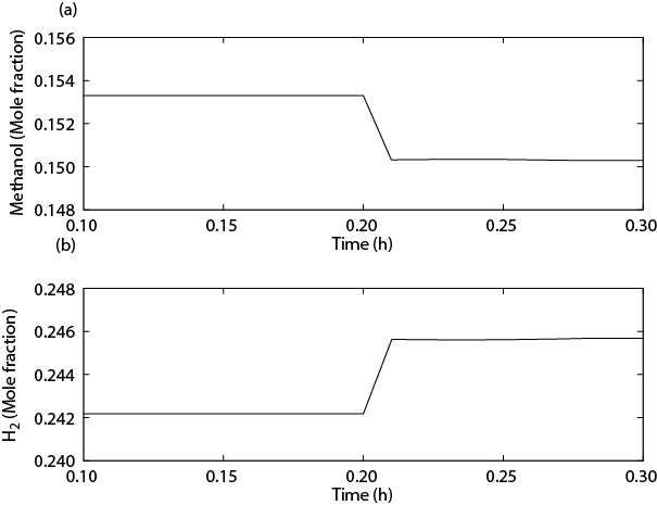
The catalyst particle density is 1800 kg/m³, and the bed voidage is 0.45. The reactor length is 5 m, and the diameter is 1 m. At steady state, the feed valve is 50% open. The feed valve is closed to 25% in a single step. Compare the dynamic responses of the methanol and H₂ concentrations at the reactor outlet by using various explicit methods (such as the explicit Euler and Runge-Kutta methods) and implicit methods (such as the implicit Euler and Gear’s method of various orders).

Solution

The problem is set up in Aspen Engineering Suite (AES) using Aspen Plus V9.0 and Aspen Plus Dynamics V9.0. The thermodynamics package used is PR EOS. The pressure drop in the reactor is calculated by the Ergun equation. It is assumed that the catalyst and the fluid are at the same temperature. The CuO/ZnO/Al₂O₃ catalyst used in this study contains about 63 wt% CuO, 25 wt% ZnO, and 12% Al₂O₃ [10]. The mass-weighted heat capacity of the catalyst is calculated to be 635 J/kg K. As the reactor model is solved in Aspen Plus Dynamics using the method of lines, the PFR is discretized into 100 grids and solved with the first-order, backward finite-difference method. Cooler E-1102 is set up using the “LMTD” option. In Aspen Plus Dynamics, when the explicit Euler method is used, the dynamic simulation could be solved only with a minimum step size of 0.4 × 10⁻⁵ s. Such a small step is obviously unacceptable. Performance of the fourth-order explicit Runge-Kutta method is slightly better, but still unacceptable. The implicit Euler method, Gear’s method of order two, and Gear’s method of order five yield similar results. Figure E17.4(b) shows the methanol and H₂ concentrations at the reactor outlet. Considering the computational expense, the implicit Euler’s method is the best choice for this system.

Two line graphs show the methanol and hydrogen concentrations at the outlet of the reactor.

Graph a has the horizontal axis labeled Time (hours), ranging from 0.10 to 0.30, in increments of 0.05, and the vertical axis labeled Methanol (Mole Fraction), ranging from 0.148 to 0.156, in increments of 0.002. The line graph begins at (0.10, 0.153), continues as a straight line to (0.20, 0.153), slopes down to (0.21, 0.150), and continues as a straight line to (0.30, 0.150). Graph b has the horizontal axis labeled Time (hours), ranging from 0.10 to 0.30, in increments of 0.05, and the vertical axis labeled Hydrogen (Mole Fraction), ranging from 0.240 to 0.248, in increments of 0.002. The line graph begins at (0.10, 0.242), continues as a straight line to (0.20, 0.242), slopes up to (0.21, 0.246), and continues as a straight line to (0.30, 0.246). All coordinate plots are approximate.

Figure E17.4(b) Transient Response at the Outlet of the Reactor: (a) Methanol Concentration (Mole Fraction); (b) H₂ Concentration (Mole Fraction)

17.4 Process Control

When there is no controller present, the dynamic response is called the open-loop response. Open-loop dynamic simulation can be performed only for open-loop-stable processes. A process is open-loop stable if the state variables return to steady-state values when one or more input variables are perturbed. For the processes that are open-loop unstable, an appropriate regulatory control layer should be designed first. The dynamic response of a closed-loop process does not only depend on the process itself but also on the control configuration and controller design. This discussion will mainly focus on lower-level, control system design that is required both for a stable simulation and for satisfying the objectives of plant operation. Only the essentials of process control needed to obtain a stable dynamic simulation are discussed here, but the interested reader can find more details on process control from several excellent books in this area [12–14].

Lower-level controllers are usually single-input-single-output (SISO) controllers. These controllers maintain a single output, known as the controlled variable (CV), at its desired value, known as the set point (SP), by manipulating a single input, known as the manipulated variable (MV). There are two objectives for the lower-level control system design, namely, set point tracking or servo control, and regulatory control or disturbance rejection. In servo control, the objective is to track a reference trajectory in the SP, while in regulatory control, the objective is to maintain the CV at the SP in face of process disturbances.

If the lower-level control system design is not appropriate, the simulation may slowly drift from its nominal operating condition or reach an undesired operating region. In the worst case, it will lead to convergence failure. For stability of the dynamic simulation, both control structure design and controller design are important.

The most common control structure is feedback control used for both the servo and regulatory functions. In feedback control, at every simulation time step, the CV is sampled and compared to the SP, and an error signal is generated. If the deviation variables (i.e., deviation from the steady-state values) for CV and SP are denoted by y_m and y_r, respectively, then the error is calculated as

\begin{matrix} ϵ = y_{r} - y_{m} \end{matrix} (17.41)

$\begin{matrix} ϵ = y_{r} - y_{m} \end{matrix} (17.41)$

The control action is almost always based on the error signal and depends upon the controller design. Most frequently a proportional-integral-derivative (PID), or a proportional-integral (PI), or a proportional-only (P-only) controller is used for calculating the control action. If the deviation variable of the control action is denoted by c and if a PID controller is used, then the control action can be written as

\begin{matrix} c (t) = K_{c} [ϵ (t) + \frac{1}{τ_{I}} \int_{0}^{t} ϵ (t) dt + τ_{D} \frac{dϵ (t)}{dt}] \end{matrix} (17.42)

$\begin{matrix} c (t) = K_{c} [ϵ (t) + \frac{1}{τ_{I}} \int_{0}^{t} ϵ (t) dt + τ_{D} \frac{dϵ (t)}{dt}] \end{matrix} (17.42)$

In Equation (17.42), K_c is the proportional gain, τ_I is the integral time or reset time, and τ_D is the derivative time constant. While designing the controller, the direction of the control action must be provided by the user. If the steady-state gain of a system is positive, that is, an increase in the input variable causes the output variable to increase, the controller gain should be positive. This is known as direct action. In contrast, for a system with negative steady-state gain, the controller gain has to be negative. This is known as reverse action.

Controller type is chosen based on the process. P-only control results in a steady-state offset, except for processes with a natural integrator, such as level control of a vessel or pressure control of a gas drum. PI control is probably the most widely used type of controller, because it eliminates any offset between the steady-state value of CV and the SP. But care must be taken as the response can become oscillatory due to an aggressive integral action. PID controllers are most suitable for processes with some delay in their response. However, the CV value should be relatively noise free for the derivative action to be used effectively without generating a noisy MV. Details are again available in standard textbooks on process control.

To achieve the desired control performance with a PID controller, its parameters, K_c, τ_I, and τ_D, should be tuned. Controller tuning is a vast and complicated subject, and interested readers are again referred to any standard textbook on process control. The parameters can be tuned manually, but a trial-and-error method may not result in a satisfactory performance. For example, for a PID controller, there is a bound on the proportional gain, K_c, beyond which the process can become unstable. Therefore, various methods are available in dynamic simulators where approximate process model/information can be used for finding the appropriate tuning parameters. Two of these methods will be discussed here, mainly because these methods are easy to apply and are typically available in process simulators. The first method is based on the use of stability margins. The second method requires an approximate process model. The first method is based on determination of the ultimate controller gain (K_cu) that brings the closed-loop process to the verge of instability. The corresponding period of sustained oscillation is known as the ultimate period of oscillation (P_u). For determining K_cu, the proportional gain of the controller can be manually increased until the process reaches sustained oscillation in response to a step change in an input. Another popular method to determine K_cu and P_u is known as autotune variation (ATV). In this method, the controller is replaced by a relay that helps to determine K_cu. Once the ultimate controller gain and ultimate period of oscillation are established, the controller tuning parameters are decided by following rules such as the Ziegler-Nichols stability margin controller tuning rule or the Tyreus-Luyben rule. In the second method, the control loop under consideration is opened, a step change in the input is introduced, and the transient response in the output is recorded. Then a simple process model, such as first-order, first-order plus time delay, or second-order plus time delay, is fitted to the process-response curve. Once the characteristic parameters of such models, such as time delay, process gain, time constant, and so forth, are extracted, there are various tuning rules, such as Cohen-Coon tuning rules or the Ziegler-Nichols tuning rule, that can be used. In summary, a stable dynamic simulation can usually be achieved by using an appropriate control structure and controller design even though the control system performance may not be satisfactory.

Example 17.5

Consider Example 17.3, where a mixture of CO₂ and methanol is separated in a jacketed flash vessel. The inlet temperature of the heating medium is 90°C, and its specific heat is similar to that of water. There is no phase change of the heating medium in the jacket. The heat transfer option in the dynamic simulation is “LMTD,” and the heating-medium flowrate is manipulated to maintain the vessel outlet temperature at 70°C, as shown in Figure E17.5(a). Figure E17.5(a) also shows that the flow dynamics of the heating medium are neglected, assuming perfect control. So there are four controllers: FC-1101, PC-1101, LC-1101, and TC-1101. Tune these controllers by using both methods mentioned before (i.e., by using stability margins and by using an approximate process model) and by applying the various rules discussed previously. Then decrease the feed flow to 50 kmol/h in a single step. Show the differences in the transient response of the outlet temperature with the controllers being tuned by different rules.

A diagram shows the configuration of the jacketed flash vessel for separating carbon-dioxide and methanol, where the flow rate of the heating fluid controls the vessel outlet temperature.

Stream 1 contains an input feed at 30 degrees Celsius, 5 bars of pressure, 100 kilomoles per hour, y subscript methanol equals 0.9, and y subscript carbon-dioxide equals 0.1. Stream 1 enters F C - 1101, which is connected to C V - 1101 directly and through an F C unit. C V - 1101 sends stream 2 to the flash vessel. The flash vessel has a layer, that forms the jacket, coating its bottom half. The vessel is labeled V-1101, has a temperature 70 degrees Celsius, and P equals 3.0 bar. Streams 3 and 5 also leave the vessel. Stream 3 is connected to C V - 1102, both directly and through a P C unit. Stream 4 from C V - 1102 produces a Vapor Product. Stream 5 from the vessel is sent to C V - 1103, which is connected back to the vessel through an L C unit. Stream 6 from C V - 1103 contains a Liquid Product. The vessel is connected to the T C unit labeled T C-1101, which in turn sends stream 7 back to the vessel through a valve. The Heating Fluid joins stream 7 through the valve. Heating Fluid is sent out from the vessel through its bottom, as stream 8. All C V valves have delta P equivalent to 1 bar.

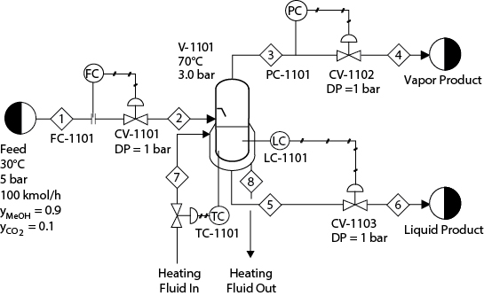
Figure E17.5(a) Configuration of the Jacketed Flash Vessel for Separating CO₂ and Methanol Where the Vessel Outlet Temperature Is Being Controlled by Manipulating the Flowrate of the Heating Fluid

Solution

As in previous problems, the problem is set up in Aspen Engineering Suite (AES) using Aspen Plus V9.0 and Aspen Plus Dynamics V9.0. The flow, pressure, and level controllers are considered to be PI controllers, and the temperature controller is considered to be a PID controller. As seen later, the time delay of the temperature loop is small; thus the derivative action can be neglected. In Aspen Plus Dynamics V9.0, both methods for controller tuning are available under the “Tune” tab of individual controllers. For the first method that uses stability margin, the test method “Closed Loop (CL) ATV” is selected. The relay amplitude is specified to be 5% of the output range. At the end of this test, K_cu and P_u are calculated automatically. Then, under the “Tuning parameters” tab, the tuning parameters are calculated based on these values of K_cu and P_u and choice of tuning rule. Ziegler-Nichols (Z-N) and Tyreus-Luyben (T-L) tuning rules are used to obtain the tuning parameters shown in Table E17.5. For the second method that uses an approximate process model, the test method “open loop” (OL) is selected. A step up by 5% of the output range is selected to be the test specification. At the end of this test, Aspen Plus Dynamics automatically identifies the characteristic parameters, that is, open-loop gain, time constant, and time delay of a first-order-plus-time-delay process. Then, under the “Tuning parameters” tab, the tuning parameters are calculated based on the values of these characteristic parameters and choice of tuning rule. Ziegler-Nichols, Cohen-Coon (C-C), IMC, IAE, ISE, and ITAE tuning rules are used to obtain the tuning parameters shown in Table E17.5.

Table E17.5 Tuning Parameters Applying the Two Methods and Various Tuning Rules

Method	Tuning Rule	FC-1101		PC-1101		LC-1101		TC-1101
Method	Tuning Rule	K_c (%/%)	τ_I (min)	K_c (%/%)	K_c (min)	K_c (%/%)	τ_I (min)	K_c (%/%)	τ_I (min)	τ_η (min)
CL
ATV	Z-N	1.71	0.09	50.61	0.11	306.34	0.09	1723.12	0.06	0.02
CL
ATV	T-L	1.17	0.25	34.79	0.29	210.61	0.25	915.41	0.29	—
OL	C-C	46.18	0.01	401.88	0.01	134.44	0.13	3151.22	0.03	0.01
OL	Z-N	31.25	0.01	401.56	0.01	134.36	0.13	2838.31	0.03	0.01
OL	IMC	3.67	0.09	12.56	0.45	3.00	6.48	16.74	1.53	0.01
OL	IAE	15.22	0.01	410.63	0.03	136.75	0.29	2342.62	0.05	0.01
OL	ISE	22.73	0.01	478.67	0.03	157.98	0.30	2731.63	0.04	0.01
OL	ITAE	21.26	0.01	343.38	0.03	114.01	0.30	2502.84	0.06	0.01

For the IMC method, the tuning parameter, λ, is considered to be 0.3 times the process time constant. Table E17.5 shows that the tuning parameters calculated by the rules under the “closed-loop ATV” method are similar. On the other hand, all the rules for the “open-loop” method calculate similar tuning parameters except the IMC method. Also, note that the gain values calculated by all the rules under the “open-loop” method are much larger. As the feed flow is step decreased to 50 kmol/h, the differences in the transient response in the outlet temperature due to various tuning rules are shown in Figures E17.5(b) and E17.5(c), respectively. In Figure E17.5(b), the transient responses for all the tuning rules except the IMC rule are shown. Figure E17.5(b) shows that the performance of all the control loops is satisfactory. However, Figure E17.5(c) shows that the deviation is comparatively large when the IMC rule is used. It should be noted that the flash vessel is the only unit operation considered in this example. In case of other unit operations being present in the same process, significant interactions may take place and many of the controller gains calculated by the various rules under the “open-loop” method may have to be decreased (“detuned”).

A graph shows the transient response of the outlet temperature using various tuning rules except for the I M C - based rule.

The horizontal axis is labeled Time (hours), ranging from 0.0 to 0.40, in increments of 0.05, and the vertical axis is labeled Outlet Temperature (degrees Celsius), ranging from 69.98 to 70.05, in increments of 00.01. All the three line graphs begin at (0.0, 70.00), run as straight lines until they rise at (0.10, 70.00) to different heights and fall, and then again continue as straight lines to (0.40, 70.00). The Cohen-Coon, Ziegler-Nichols, and Time-Integral Tuning Rules graph rises to the point (0.10, 70.01), and falls to (0.11, 69.999), and joins the straight line. The All Tyreus-Luyben Tuning Rule graph rises to the point (0.10, 70.025), and joins the straight line at (70.00, 0.12). The Ziegler-Nichols Stability Margin Tuning Rule graph rises to (0.10, 70.04), and joins the straight line at (0.135, 70.00). All coordinate plots are approximate.

Figure E17.5(b) Transient Response of the Outlet Temperature Using Various Tuning Rules Except the IMC−Based Rule

A graph shows the transient response of the outlet temperature using various tuning rules including the I M C - based rule.

Figure E17.5(c) Transient Response of the Outlet Temperature Using Various Tuning Rules Including the IMC−Based Rule

Example 17.6 demonstrates that a dynamic simulation can be used to study important changes in the transient response that may occur in the course of plant operations. Such studies can help to avoid potentially unsafe plant operations.

Example 17.6

Figure E17.6(a) shows the schematic of a cooled tubular reactor in which maleic anhydride is being produced by oxidizing benzene [15]. This problem is similar to the problem in Appendix B.5. However, there are some differences in the problem specification in this example compared to that in Appendix B.5. Ignoring the quinine formation reaction in Appendix B.5, the following reactions are considered:

A figure shows the configuration of the cooled tubular reactor for producing Maleic Anhydride from Benzene.

Stream 1 contains Air at 510 degrees Celsius, 2.75 bars of pressure, and 0.20 kilomoles per hour. Stream 1 enters FC-1102, which is connected to C V - 1104 directly and through an F C unit. The output from C V - 1104 is stream 2. The F C unit is connected to a Y C unit through a Remote Set Point. The Y C unit, labeled Y C-1101 benzene concentration connects to stream 2. Stream 3 contains Pure Benzene at 510 degrees Celsius, 2.75 bars of pressure, and 0.001 kilomoles per hour. Stream 3 enters F C - 1103, which is connected to C V - 1105 directly and through an F C unit. The output from C V - 1105 is stream 4. Stream 4 also connect to stream 2, to give stream 5, which is input to the reactor. The reactor is labeled R-1102, where epsilon equals 0.4. The reactor releases stream 6, which passes through V L V - 1104 to produce stream 7, that is the Product at a pressure of 1.72 bars. Stream 8 contains Steam at 49 degrees Celsius and 143.6 bars of pressure. Stream 8 enters F C - 1104, which is connected to C V - 1106 directly and through an F C unit. The output from C V - 1106 is stream 9, which enters the reactor. The reactor releases stream 10, which passes through V L V - 1105 to produce stream 11, that is Steam at a pressure of 142.2 bars. All C V valves have delta P equivalent to 0.82 bars.

Figure E17.6(a) Configuration of the Cooled Tubular Reactor for Producing Maleic Anhydride from Benzene

\begin{matrix} C_{6} H_{6} + 4.5 O_{2} \to C_{4} H_{2} O_{3} + 2 C O_{2} + 2 H_{2} O \\ C_{6} H_{6} + 7.5 O_{2} \to 6 C O_{2} + 3 H_{2} O \\ C_{4} H_{2} O_{3} + 3 O_{2} \to 4 C O_{2} + H_{2} O \end{matrix}

$\begin{matrix} C_{6} H_{6} + 4.5 O_{2} \to C_{4} H_{2} O_{3} + 2 C O_{2} + 2 H_{2} O \\ C_{6} H_{6} + 7.5 O_{2} \to 6 C O_{2} + 3 H_{2} O \\ C_{4} H_{2} O_{3} + 3 O_{2} \to 4 C O_{2} + H_{2} O \end{matrix}$

These reactions are carried out using excess air to avoid runaway reactions. As a result, the reactions can be considered as pseudo-first-order reactions. The reaction rates can be written as [15]

\begin{matrix} k_{1} = 4280 exp [\frac{- 12,660}{T (K)}] \frac{m^{3}}{kg cat s} \\ k_{2} = 70,100 exp [\frac{- 15,000}{T (K)}] \frac{m^{3}}{kg cat s} \\ k_{3} = 26 exp [\frac{- 10,800}{T (K)}] \frac{m^{3}}{kg cat s} \end{matrix}

$\begin{matrix} k_{1} = 4280 exp [\frac{- 12,660}{T (K)}] \frac{m^{3}}{kg cat s} \\ k_{2} = 70,100 exp [\frac{- 15,000}{T (K)}] \frac{m^{3}}{kg cat s} \\ k_{3} = 26 exp [\frac{- 10,800}{T (K)}] \frac{m^{3}}{kg cat s} \end{matrix}$

Since these reactions are highly exothermic, a molten, eutectic salt is circulated in a multitube reactor to maintain the desired temperature. For simplicity, it can be assumed that an excess amount of steam is used to cool the reactor such that the change in the steam temperature during steady-state operation is not significant. This results in a nearly isothermal operation of the reactor. The reactor size is the same as recommended in the work of Westerink and Westerterp [15]. This gives the length and diameter of a single tube to be 12.8 m and 0.028 m, respectively. The pressure drop across the reactor on both the process and cooling-medium sides can be considered negligible. Catalyst density is 900 kg/m³. Assume SS302 (stainless steel type 302) to be the material of construction. Heat loss to the ambient can be assumed to be negligible.

Develop a dynamic simulation of this cooled tubular reactor assuming that the dimensions of the reactor are that of a single tube. Implement the controllers as shown in Figure E17.6(a). Assume the overall heat transfer coefficient (U) to be 25 W/m²°C. Then increase the flowrate of benzene to 0.0033 kmol/h while keeping the flowrate of air constant. Show the transient response of the temperature and the benzene and CO₂ concentrations at the exit of the reactor.
Now assume that the overall heat transfer coefficient (U) changes to 2 W/m²°C due to fouling. Again, increase the flowrate of benzene to 0.0033 kmol/h, keeping the air flowrate constant as before. Compare the results with those obtained previously.

Solution

The simulation is set up in Dynsim 4.5.3 using the SRK EOS. In Dynsim, three “sink” blocks are used for the sources of air, benzene, and steam, respectively, and kinetic reactions can be simulated in a number of blocks; however, because of the presence of the cooling jacket and the catalyst in the reactor, a PFR block is chosen. The thickness of the reactor wall is calculated as in Example E17.3, considering SS302 as the material of construction. For specifying the pressure drop of a stream in a block, Dynsim provides the option to provide the flow conductance. The flow conductances of the flow and reaction passes of the PFR are provided as 150 kg/s/(kPa kg/m³)^0.5. Three “reaction data sets” are created for modeling the kinetics of the reactions. The “reaction data sets” can be created in Dynsim 4.5.3 by clicking “RDS” under the “Process Equipment” tab of the “Icon Palette.” These data sets are then associated with a reaction set. The reaction set block is known as “RD” in Dynsim and is available under the “Process Equipment” tab of the “Icon Palette.” This reaction set is then enabled under the “Reactions” tab of the PFR. Three “PID” blocks available under the “Controls” tab of the “Icon Palette” are used for the controllers FC-1102, FC-1103, YC-1101, and FC-1104, respectively. Keeping the set point of FC-1102 constant, CV-1105 is manually opened to achieve a step change in the flowrate of the benzene feed. Figure E17.6(b) shows that the change in the temperature is negligible at the reactor outlet. The corresponding concentrations of benzene and CO₂ at the reactor outlet are shown in Figures E17.6(c)(a) and E17.6(c)(b), respectively. The benzene concentration increases at the reactor outlet while the change in the CO₂ concentration is negligible.

The horizontal axis is labeled Time (minutes), ranging from 0 to 20, in increments of 2, and the vertical axis is labeled Reactor Outlet Temperature (degrees Celsius), ranging from 400 to 1600, in increments of 200. The graph pertaining to U equals 2 watts per meter squares degrees Celsius, begins at (0, 500), starts to rise at (4, 500), reaches a peak at (5.9, 1600), falls to (7, 1450), and continues as a slight curve up to (19, 1500). The graph pertaining to U equals 25 watts per meter squared degrees Celsius, runs parallel to the horizontal axis from (0, 490). All coordinate plots are approximate.

Figure E17.6(b) Transients in Reactor Outlet Temperature with Different Overall Heat Transfer Coefficients When the Benzene Concentration in the Feed Is Changed

Graph a has the horizontal axis labeled Time (hours), ranging from 0 to 20, in increments of 2, and the vertical axis labeled Benzene Concentration at the Reactor Outlet (Mole percentage), ranging from 0 to 1.5, in increments of 0.5. The graph pertaining to U equals 2 watts per meter squares degrees Celsius, begins at (0, 0.49), starts to rise gradually at (4, 0.49) up to (6, 1.4), where it turns right and continues as a straight line parallel to the horizontal axis up to (19, 1.4). The graph pertaining to U equals 25 watts per meter squared degrees Celsius, also begins at (0, 0.49), starts to rise gradually at (4, 0.49) up to (5.5, 1.0), where it drops instantly to (5.5, 0). Graph b has the horizontal axis labeled Time (hours), ranging from 0 to 20, in increments of 5, and the vertical axis labeled Carbon-dioxide Concentration at the Reactor Outlet (Mole percentage), ranging from 0 to 10, in increments of 2. The graph pertaining to U equals 2 watts per meter squares degrees Celsius, begins at (0, 0), starts to rise gradually at (4, 0) up to (5.5, 9), where it turns right and continues as a straight line parallel to the horizontal axis up to (19, 9.9). The graph pertaining to U equals 25 watts per meter squared degrees Celsius, also begins at (0, 0), rises slightly to (4, 0.2), and continues as a straight line parallel to the horizontal axis. All coordinate plots are approximate.

Figure E17.6(c) Concentration at the Reactor Outlet with Different Overall Heat Transfer Coefficients When the Benzene Concentration in the Feed Is Changed: (a) Benzene Concentration; (b) CO₂ Concentration
The overall heat transfer coefficient is now changed to 2 W/m²°C. After making changes in an existing Dynsim simulation, the “LF” button must be clicked to load the simulation again. The simulation freezes at this point, and it can be restarted again. Once again, the previous steady-state snapshot is loaded by clicking the “IC” button and then selecting and loading the appropriate “IC” (initial condition) file. Due to the changed overall heat transfer coefficient, the exit temperature and composition will be different from before. The simulation is run for about 10 minutes, so that the process reaches its new steady state. It is noted in Figures E17.6(b) and E17.6(c)(a) that these initial conditions are different from before. Now, as before, the set point of FC-1102 remains constant, and CV-1105 is manually opened to achieve a step change in the flow of benzene feed. The transient responses of the temperature and the benzene and CO₂ concentration are plotted in Figures E17.6(b), E17.6(c)(a), and E17.6(c)(b), respectively. Figure E17.6(b) shows that a temperature runaway has taken place. Figure E17.6(c)(a) shows that the benzene is almost entirely consumed due to Reaction 2, as reflected by a large increase in CO₂ shown in Figure E17.6(c)(b). In this process, Reaction 1 is dominant at lower temperatures while Reaction 2 is dominant at higher temperatures, causing a runaway oxidation reaction due to the presence of a large amount of excess air. According to the work of Westerink and Westerterp [15], a dimensionless group that is representative of the ratio between the heat withdrawal rate and the maximum heat generation rate must be larger than a desired value to avoid unsafe conditions for this reactor. As the feed rate is increased, the rate of heat generation becomes higher. However, when the overall heat transfer coefficient is 2 W/m²°C, the heat removal rate is lower than the heat generation rate. Thus, the reactor temperature keeps increasing gradually, followed by a sharp rise in the temperature due to the fast oxidation reaction.

17.5 Summary

Dynamic simulations can provide information about the transient trajectory of a process that can be effectively used for a number of applications. In this chapter, various steps required for setting up dynamic simulations in a process simulator were discussed. Necessary data and specifications required for simulating realistic transient responses were covered. Troubleshooting stability issues and convergence failures of dynamic simulations are difficult and complicated. To this end, a number of issues were discussed with respect to both problem setup as well as choice of algorithms. A brief demonstration of process control shows how the performance of the control system varies based on the controller tuning parameters. Last, it should be noted, for a robust dynamic simulation such that it does not fail to converge in the face of a wide range of disturbances of varying magnitudes, all three components—the problem setup and its specification, the control system design, and the solver algorithms—must be carefully addressed.

WHAT YOU SHOULD HAVE LEARNED

The steps required for developing a stable dynamic simulation starting with a steady-state simulation involve
- Topological changes in the steady-state simulation
- Design of the equipment size and geometry
- Additional dynamic specifications
- Control systems design
- Choice of appropriate solver algorithms
Dynamic specifications should be carefully chosen from the options available in a simulator to avoid unrealistic transient responses.
An implicit adaptive method of order between 2 and 4 is usually a very good choice for the integrator algorithm.
A number of methods are available for calculating controller tuning parameters. However, the control system performance can vary widely based on the method chosen.

References

1. Coker, A. K., Ludwig’s Applied Process Design for Chemical and Petrochemical Plants, Vol. 1, 4th ed. (Burlington, MA: Gulf Professional Publishing, 2007).

2. Coker, A. K., Ludwig’s Applied Process Design for Chemical and Petrochemical Plants, Vol. 2, 4th ed. (Burlington, MA: Gulf Professional Publishing, 2010).

3. Walas, S. M., Chemical Process Equipment: Selection and Design (Stoneham, MA: Butterworth, 1988).

4. Luyben, W., Plantwide Dynamic Simulators in Chemical Processing and Control (New York: Marcel Dekker, 2002).

5. Fogler, H. S., Elements of Chemical Reaction Engineering, 4th ed. (Upper Saddle River, NJ: Prentice Hall PTR, 2005).

6. Levenspiel, O., Chemical Reaction Engineering, 3rd ed. (New York: John Wiley & Sons, 1998).

7. Taylor, R., and R. Krishna, Multicomponent Mass Transfer (New York: John Wiley & Sons, 1993).

8. Rademaker, O. J., J. E. Rijnsdorp, and A. Maarleveld, Dynamics and Control of Continuous Distillation Column (Amsterdam, The Netherlands: Elsevier, 1975).

9. Shinskey, F. G., Distillation Control (New York: McGraw-Hill, 1984).

10. Šetinc, M., and J. Levec, “On the Kinetics of Liquid-Phase Methanol Synthesis over Commercial Cu/ZnO/Al₂O₃ Catalyst,” Chem. Eng. Sci. 54 (1999): 3577–3586.

11. Newton, R. H., and B. F. Dodge, “The Equilibrium between Carbon Monoxide, Hydrogen, Formaldehyde, and Methanol: I. The Reactions CO + H₂ ⇌ HCOH and H₂ + HCOH ⇌ CH₃OH” J. Am. Chem. Soc. 55 (1933): 4747–4759.

12. Ogunnaike, B. A., and W. H. Ray, Process Dynamics, Modeling, and Control (New York: Oxford University Press, 1994).

13. Coughanowr, D. R., Process Systems Analysis and Control, 2nd ed. (New York: McGraw-Hill, 1991).

14. Bequette, B. W., Process Control: Modeling, Design, and Simulation (Upper Saddle River, NJ: Prentice Hall PTR, 2003).

15. Westerink, E. J., and K. R. Westerterp, “Safe Design of Cooled Tubular Reactors for Exothermic Multiple Reactions: Multiple Reaction Networks,” Chem. Eng. Sci. 43 (1988): 1051–1069.

Short Answer Questions

1. What information about a process can be obtained from a dynamic simulation that is not possible to obtain from a steady-state simulation?

2. For obtaining a valid pressure-flow network, why should the pressure nodes be connected through flow devices?

3. Two flash vessels have the same length (L) but different diameters (D). Both vessels contain the same material and have the same operating pressure and temperature. In both vessels, the liquid level is being maintained at 50% by manipulating a control valve at the bottom of the flash vessel. If both vessels are horizontal, at the inlet of which control valve will you expect the higher pressure? Why? What happens if the vessels are vertical?

4. In a process, it is desired to manipulate the refrigerant flowrate to a cooler to maintain the cooler outlet temperature. What heat transfer option would you choose for developing a dynamic model of this cooler?

5. In a cooler, cooling water is being used to cool a process stream. It is desired to maintain the proces stream outlet temperature. What will be the CV and MV of the controller? Due to the water quality, it is suggested that the cooling water outlet temperature should not exceed 45^oC. What type of controller should be designed and how will it be ensured that the constraint on cooling water temperature is not violated?

6. In a reactor, it is known that a fast reaction takes place in the initial region combined with a slower reaction that occurs over the entire length of the reactor. What will be a computationally efficient way of modeling this reactor? (Hint: A single reactor or a combination of reactors?) For solving this problem, which integrator algorithm would you choose? Why?

7. When the fuel flow to a furnace is varied, in response the furnace outlet temperature changes after some time. The outlet temperature signal is noisy. Would you use a PID controller for this process? If yes, explain what other issues should be addressed and how.

Problems

8. Consider Example 17.5, where a mixture of CO₂ and methanol is being separated in a jacketed flash vessel. The heat content in the bottom product from the flash vessel is now recovered in heat exchanger E-1103, as shown in Figure P17.8. Note the difference in the inlet feed pressure compared to Example 17.5, which is included to take care of the pressure drop in the exchanger, E-1103. Also note the changed location of the control valve, CV-1103, used for level control of V-1102. The remainder of the specifications are the same as in Example 17.5. For this problem do the following:

A diagram shows the configuration of the jacketed flash vessel for separating carbon-dioxide and methanol, with a bottom feed heat exchanger.

Stream 1 contains an input feed at 30 degrees Celsius, 5 bars of pressure, 100 kilomoles per hour, y subscript methanol equals 0.9, and y subscript carbon-dioxide equals 0.1. Stream 1 enters F C - 1101, which is connected to C V - 1101 directly and through an F C unit. C V - 1101 sends stream 2 to the heat exchanger, which in turn is connected to the flash vessel. The flash vessel has a layer, that forms the jacket, coating its bottom half. The vessel is labeled V-1101, has a temperature of 70 degrees Celsius, and a pressure of 3.0 bars. Streams 3, 5 and 8 leave the vessel. Stream 3 is connected to C V - 1102, both directly and through a PC unit. Stream 4 from C V - 1102 produces a Vapor Product. Stream 5 from the vessel is sent back to the heat exchanger. Stream 6 from the heat exchanger is passed on to C V -1103, which is connected back to the vessel through an L C unit labeled L C 1101. Another part of stream 6 from C V - 1103 contains a Liquid Product. The vessel is connected to the T C unit labeled T C - 1101, which in turn sends stream 7 back to the vessel through a valve. The Heating Fluid joins stream 7 through this valve. Heating Fluid is sent out from the vessel through its bottom, as stream 8. All C V valves have delta P equivalent to 1 bar.

Figure P17.8 Configuration of the Jacketed Flash Vessel for Separating CO₂ and Methanol with a Bottom/Feed Heat Exchanger

Develop a “rigorous” design of the heat exchanger, E-1103, considering a maximum pressure drop of 0.1 bar in the shell and tube sides and a minimum temperature approach of 15°C.
Tune the four controllers, FC-1101, TC-1101, PC-1101, and LC-1101, by using both of the methods mentioned in Chapter 17 (i.e., by using stability margins and by using an approximate process model) and applying various rules similar to those used in Example 17.5. Did the tuning parametesrs differ from the ones in Example 17.5? If they did differ, explain why.
Step decrease the feed flow to 40 kmol/h. Show the differences in the transient response in the level controller with the controllers being tuned by different rules.
Use the tuning parameters for which you obtained the “best” performance in Part (c). The process is again at set at steady state with 100 kmol/h feed flowrate. Keep increasing the proportional gain of the level controller, LC-1101, each time by 30% up to 150% of the original gain. For each value of the proportional gain, step decrease the feed flow from 100 kmol/h to 40 kmol/h. Even though the tuning of the temperature controller, TC-1101, was not altered, did you notice any change in its performance? Why does this happen? Take corrective action such that the performance of the TC is similar to what it was before.

9. Consider Example 17.4, in which methanol is produced in a PFR. After being cooled, the reactor effluent is now sent to a flash vessel, V-1103, as shown in Figure P17.9. The overhead gas stream from V-1103 is sent to a compressor where it is compressed to 15 bar. The bottom liquid is pumped by P-1101. The control valve, CV-1105, is used for maintaining the level of V-1103. The material of construction is carbon steel for all equipment. Assume the compressor to be isentropic with 80% efficiency. The efficiency of P-1101 is also 80%.

Stream 1 consists of Syngas Feed at 250 degrees Celsius, 3 bars of pressure, and 100 kilomoles per hour. Stream 1 enters F C - 1102, which is connected to C V - 1104 directly and through an F C unit, labeled F C 1102. C V - 1104 sends stream 2 to the reactor along with a Coolant input. The reactor is labeled R-1101, and has a length and diameter that equals 5 and 1 meters, respectively. Coolant is sent out from the reactor. Stream 3 is also released from the reactor and sent to E-1102. Stream 4 at 40 degrees Celsius is released from E-1102 and is sent to the flash vessel. Stream 5 from the vessel is connected to C-1101 both directly and through a P C unit, labeled P C 1102. C-1101 is labeled Set Point for Compressor Power. It releases stream 6 that contains the Vapor Product at 15 bars of pressure. Stream 7 from the vessel is sent to P-1101, that has the delta P value as 8 bars. Stream 8 from here is sent to C V 1105, which is connected to an L C unit labeled L C 1102. The L C unit is connected to the flash vessel. A part of stream 8 entering C V 1105 leaves it as stream 9 that contains a Liquid Product.

Figure P17.9 Configuration of a Section for Producing Methanol from Syngas

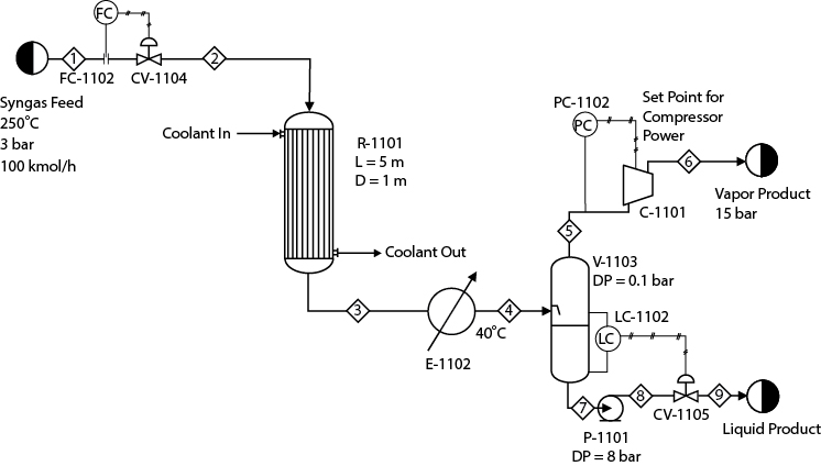
Develop a steady-state model of the process.
Develop a dynamic model. Size the required equipment following the heuristics provided in Chapter 11. Consider the metal mass of V-1103. Heat loss to the environment can be assumed to be negligible. Tune the controllers FC-1102, LC-1102, and PC-1102 one at a time. Now step decrease the syngas flow to 60 kmol/h. As you have tuned the controllers one at a time, does it perform satisfactorily when the controllers interact with each other? If not, what changes should you make to achieve satisfactory performance in case of loop interactions?
Now double the proportional gain of PC-1102. What happens to the performance of LC-1102? Why? Retune LC-1102 to achieve satisfactory performance.

10. Figure P17.10 shows a simplified configuration of a steam generation system. In combustor R-1102, the following reaction takes place:

An illustration of a simplified steam generation system.

Stream 1 consists of Methane at 2.5 bars of pressure, 100 degrees Celsius, and 500 kilomoles per hour which is sent to F C 1103. F C 1103 is connected to C V 1106 both directly and through an F C unit. Stream 2 from C V 1106 is sent to the reactor, R-1102, that has a delta P value equivalent to 0.1 bars. Stream 3 consists of Methane at 2.5 bars of pressure, 60 degrees Celsius, and 6666 kilomoles per hour which is sent to F C 1104. F C 1104 is connected to C V 1104 both directly and through an F C unit. Stream 4 from C V 1104 is sent to the reactor, R-1102. An X C unit labeled XC-1101, connects the two F C units. Stream 5 is sent from the reactor to E-1104, that sends stream 6 to E-1105. Stream 7 is sent from E-1105 to E-1106, which sends stream 8 to V L V 1111, that has delta P value equivalent to 0.1 bars. Stream 9 is released from here, containing Flue Gas to Stack. Stream 10 consists of B F W at 42 bars and 100 degrees Celsius that is sent to the F C unit, labeled F C 1105, and to C V 1108. Stream 11 from C V 1108 is sent to E-1106. Stream 12 from E-1106 enters the steam drum below, which is connected to an L C unit, L C 1103. F C 1105 is connected to L C 1103 by a dashed line labeled Remote sp. Stream 13 leaves the steam drum through its bottom and splits into streams 16 and 14. Stream 14 is sent to F C 1106, which is connected both directly and through an F C circuit to C V 1109. Stream 15 from here is sent to the Blowdown. Stream 16 enters P-1102, which sends stream 17 to F C 1107, which is connected to C V 1110 directly and through an F C unit. Stream 18 is sent from C V 1110 pt E-1105, which sends stream 19 back to the steam drum. Stream 20 is sent from the stream drum to E-1104, which produces stream 21. Stream 21 is connected to C V 1111 both directly and through a P C unit, labeled P C 1103. Stream 22 containing Superheated Steam, is released from C V 1111. All C V valves have delta P equivalent to 1 bar.

Figure P17.10 Configuration of a Simplified Steam Generation System

C H_{4} + 2 O_{2} \to C O_{2} + 2 H_{2} O

$C H_{4} + 2 O_{2} \to C O_{2} + 2 H_{2} O$

Complete conversion of the fuel gas in R-1102 can be assumed. Flue gas from the combustor goes to the superheater, E-1104, followed by the steam generator, E-1105. Finally, the flue gas flows through the economizer, E-1006, before going to the stack. The bfw flows through E-1006 before reaching the steam drum, V-1104. A portion of the bottom steam from the steam drum goes to the blowdown. The other portion goes to pump P-1102 and then to E-1105. The differential pressure across P-1102 should be equal to the pressure drop across CV-1110 and E-1105. The exit stream from E-1105 returns to V-1104. The pressure drop in V-1104 can be neglected. The generated steam gets superheated in E-1104 before leaving the unit. The degree of superheat in E-1104 is 100°C. Assume Stream 19 is 99% vapor. V-1104 may be considered to be adiabatic.

First, develop a steady-state model of this process. Simulate E-1104, E-1105, and E-1106 as “rigorous” heat exchangers. (Note that the pressure drop across the heat exchangers is not provided in the problem statement since it should be determined by the detailed design of these exchangers.) Implement two design specifications. The first design specification manipulates the flow of bfw, Stream 10, to ensure that the temperature of Stream 8 is 150°C to avoid “cold-end” corrosion. The other design specification manipulates the flowrate of the circulating water, Stream 16, so that the flowrate of the blowdown stream, Stream 14, is 1% of the bfw feed, Stream 10. (Note: Because of the recycle loop, the design specifications, and the rigorous heat exchangers and due to the strong interaction between the design specifications, the steady-state simulation is difficult to converge unless appropriate convergence options are chosen. Refer to Section 16.3 for a discussion and approaches to solving such problems.)
Develop a dynamic model of this system. For E-1104, E-1105, and E-1106, provide the shell-side and tube-side volumes and the metal mass of each side. Heat loss to the environment for all equipment can be neglected. Size V-1104 following the heuristics in Chapter 11. Figure P17.10 shows that the air flowrate to R-1102 is regulated by a ratio controller, XC-1101, that maintains the molar ratio between fuel and air at the steady-state value. LC-1103 is cascaded with FC-1105 to maintain the level of V-1104. Information on cascaded loops and ratio controllers is available in Chapter 18. Tune the controllers with various methods and rules and compare their performance by simulating a 20% step increase in the fuel flowrate. Performance of all the controllers should be considered, especially that of LC-1103 and PC-1103.
Compare the performance of various integrator algorithms for this problem.
In Part (b), the performance of all the controllers has been considered for a 20% step increase in the fuel flowrate. Now consider simultaneously a 20% step decrease in the fuel flowrate as well as a step increase to the set point of PC-1103 by 0.5 bar. Did the same set(s) of controller tuning parameters that performed satisfactorily before again perform satisfactorily? If not, why? If the tuning parameters need to be changed, ensure that you are satisfied with the performance of the control system for both Part (b) of this problem and the current problem.

11. Consider Problem 17.10. Show the effect of the metal mass on the temperature transients during shutdown. To show this, ramp down the fuel flowrate to 20% of its steady-state value in 4 h and then completely close the fuel control valve, CV-1106. The air continues to flow with the flowrate being the same as when the fuel flowrate was 20%. Show the temperature transients of Streams 6 and 7. Now increase the metal mass of E-1104 and E-1105 by 50%. Carry out the same test again. Compare the temperature transients with what you obtained before.

12. Figure P17.12 shows the surge control loop of a compressor. The condensate in the feed and recycle stream is drained from V-1105. Then the feed gas is compressed to 25 bar in a compressor and sent to a knockout drum, V-1106. The condensate-free gas from the top of V-1106 is split into two portions. One portion goes out as product while the other portion is recycled to the compressor suction to prevent surge.

An illustration of the surge control loop of a compressor is shown.

Stream 1 consists of a Feed at 40 degrees Celsius, 3 bars of pressure, 100 kilomoles per hour, where benzene equals 0.02, toluene equals 0.03, and methane equals 0.95. The feed enters V L V 1105, that in turn sends stream 2 to the vessel V-1105, where delta Q equals 0 and delta P equals 0.01 bars. Two streams 3 and 5 are released from the vessel. Stream 3 is sent to C V 1112, where delta P equals 0.1 bars. C V 1112 produces a Condensate represented by stream 4. C V 1112 is connected to the vessel through an L C unit labeled L C 1104. Stream 5 leaves the reactor and enters the compressor C-1102, where P subscript out equals 25 bar. Stream 5 is also connected to the compressor through a P C unit labeled P C 1104. Stream 6 leaves the compressor and enters E01107, where T subscript out equals 42 degrees Celsius and delta P equals 0.1 bars. Stream 7 flows from E-1107 to vessel V-1106, where delta Q equals 0 and delta P equals 0.1 bar. Stream 8 flows from V-1106 to C V 1113, where delta P equals 0.1 bars. C V 1113 is connected to an L C unit labeled L C 1105. This is connected to vessel V-1106. Stream 10 from V-1106 splits into two streams 11 and 13. Stream 11 is sent to C V 1114, that in turn sends stream 12 to vessel V-1105. C V 1114 is also connected F C 1108. Stream 13 is connected to C V 1115 both directly and through a P C unit, labeled P C 1105. Stream 14 containing a Vapor Product is released from C V 1115.

Figure P17.12 Surge Control Loop of a Compressor

Develop a steady-state model of this system. The suggested thermo-package is PR EOS. The isentropic efficiency of C-1102 is 80%. At steady state, there is no recycle flow; that is, flow of Stream 11 is zero.
Develop a dynamic model of this system. Heat loss to the environment for all equipment can be neglected. Size V-1105 and V-1106 following the heuristics in Chapter 11. In Figure P17.12, FC-1108 is the anti-surge controller. Compressor surge control algorithms, in general, can be very involved. For simplicity, it can be assumed that if the molar flowrate of Stream 5 can be maintained within 90% of its steady-state value, a surge can be prevented. Therefore, in case of a disturbance, FC-1108 should be able to maintain the flow of Stream 5 within 90% of its set point. When sizing CV-1114, it should be ensured that it can maintain the required flow of Stream 5 even if the flowrate of Stream 1 becomes zero. Determine the “best” set of tuning parameters that provides satisfactory performance when VLV-1105 is completely closed. To reiterate the control performance requirement, the flow of Stream 5 should be maintained within 90% of its steady-state value with no or negligible oscillation. This constraint should be satisfied along with satisfactory performance of PC-1104, PC-1105, and LC-1105.
In Part (b), if performance of any or some of these controllers is not satisfactory, what would you suggest for improvement? You may suggest hardware modification(s).
For this system, it is known that the pressure of Stream 1 may increase up to 3.2 bar under certain circumstances. To check the performance of the control system for this disturbance, again consider that the process is at steady state with the flow of Stream 1 being at 100 kmol/h. Now increase the pressure of Stream 1 from 3 bar to 3.2 bar. Do you get satisfactory performance with the previous tuning parameters, especially for LC-1105 and PC-1105? If not, why?
What would be your suggested overall improvement in the process design, including control system improvement and hardware modification, so that the control system performance is satisfactory for the disturbance considered in Part (b) and in this problem? Implement your suggestions and compare the performance of the control system with the performance that you obtained before.

13. Consider Figure E17.6(a), in which the overall heat transfer coefficient (U) is assumed to be 25 W/m²°C. It can be noted that in Figures E17.6(b) and E17.6(c)(b), the transients in exit temperature and CO₂ concentration appear to be negligible. Now increase the flowrate of benzene to 0.01 kmol/h, while keeping the flowrate of air constant. Simultaneously increase the temperature of air to 520°C. Did you notice any difference in the transient profile of temperature and benzene and CO₂ concentration at the exit of the reactor compared to what is obtained in Example 17.6? Why or why not?

14. Consider Problem 17.13. Now consider the overall heat transfer coefficient (U) to be 100 W/m²°C, as suggested in Appendix B.5. Simulate the same changes as before. Did you notice any difference in the transient profiles in comparison to what you obtained before? Why or why not?

..................Content has been hidden....................

You can't read the all page of ebook, please click here login for view all page.

Table of Contents for Chapter 17 Using Dynamic Simulators in Process Design

Create new playlist

Sign In

Sign Up

Chapter 17: Using Dynamic Simulators in Process Design

17.1 Why is there a Need for Dynamic Simulation?

17.2 Setting up a Dynamic Simulation

17.2.1 Step 1: Topological Change in the Steady-State Simulation

17.2.2 Step 2: Equipment Geometry and Size

17.2.3 Step 3: Additional Dynamic Data/Dynamic Specification

17.3 Dynamic Simulation Solution Methods

17.3.1 Initialization

17.3.2 Solution of the DAE System

17.4 Process Control

17.5 Summary

References

Short Answer Questions

Problems

Table of Contents for
Chapter 17 Using Dynamic Simulators in Process Design