Chapter 19 Process Fluid Mechanics

Search in book...
Toggle Font Controls
Create new playlist

Name your new playlist

Playlist description (optional)
Sign In

Email address

Password

Forgot Password?

or

Continue with Facebook

Continue with Google
Sign Up

Full Name

Email address

Confirm Email Address

Password

or

Continue with Facebook

Continue with Google

Chapter 19: Process Fluid Mechanics

WHAT YOU WILL LEARN

The basic relationships for fluid flow—mass, energy, and force balances
The primary types of fluid flow equipment—pipes, pumps, compressors, valves
How to design a system for incompressible and compressible frictional flow of fluid in pipes
How to design a system for frictional flow of fluid with submerged objects
Methods for flow measurement
How to analyze existing fluid flow equipment
How to use the concept of net positive suction head (NPSH) to ensure safe and appropriate pump operation
The analysis of pump and system curves
How to use compressor curves and when to use compressor staging

The purpose of this chapter is to introduce the concepts needed to design piping systems, including pumps, compressors, turbines, valves, and other components, and to evaluate the performance of these systems once designed and implemented. The scope is limited to steady-state situations. Derivations are minimized, and the emphasis is on providing a set of useful, working equations that can be used to design and evaluate the performance of piping systems.

19.1 Basic Relationships in Fluid Mechanics

In expressing the basic relationships for fluid flow, a general control volume is used, as illustrated in Figure 19.1. This control volume can be the fluid inside the pipes and equipment connected by the pipes, with the possibility of multiple inputs and multiple outputs. For the simple case of one input and one output, the subscript 1 refers to the upstream side and the subscript 2 refers to the downstream side.

A figure showing the General Control Volume m, that is represented by an indefinitely shaped object. Three arrows point to the object from the left and from the object to the right.

Figure 19.1 General Control Volume

19.1.1 Mass Balance

At steady state, mass is conserved, so the total mass flowrate ( $\dot{m}$ , mass/time) in must equal the total mass flowrate out. For a device with m inputs and n outputs, the appropriate relationship is given by Equation (19.1). For a single input and single output, Equation (19.2) is used.

$\begin{matrix} \sum_{i = 1}^{m} {\dot{m}}_{i, in} = \sum_{i = 1}^{m} {\dot{m}}_{i, out} \end{matrix} (19.1)$

$\begin{matrix} {\dot{m}}_{1} = {\dot{m}}_{2} \end{matrix} (19.2)$

In describing fluid flow, it is necessary to write the mass flowrate in terms of both volumetric flowrate ( $\dot{v}$ , volume/time) and velocity (u, length/time). These relationships are

$\begin{matrix} \dot{m} = ρ \dot{v} = ρ Au \end{matrix} (19.3)$

where ρ is the density (mass/volume) and A is the cross-sectional area for flow (length²). From Equation (19.3), for an incompressible fluid (constant density) at steady state, the volumetric flowrate is constant, and the velocity is constant for a constant cross-sectional area for flow. However, for a compressible fluid flowing with constant cross-sectional area, if the density changes, the volumetric flowrate and velocity both change in the opposite direction, since the mass flowrate is constant. Accordingly, if the density decreases, the volumetric flowrate and velocity both increase. For problems involving compressible flow, it is useful to define the superficial mass velocity, G (mass/area/time), as

$\begin{matrix} G = \frac{\dot{m}}{A} = ρ u \end{matrix} (19.4)$

The advantage of defining a superficial mass velocity is that it is constant for steady-state flow in a constant cross-sectional area, unlike density and velocity, and it shows that the product of density and velocity remains constant.

For a system with multiple inputs and/or multiple outputs at steady state, as is illustrated in Figure 19.2, the total mass flowrate into the system must equal the total mass flowrate out, Equation (19.1). However, the output mass flowrate in each section differs depending on the size, length, and elevation of the piping involved. These problems are discussed later.

A figure shows the system with multiple inputs and outputs.

Figure 19.2 System with Multiple Inputs and Outputs

Example 19.1

Two streams of crude oil (specific gravity of 0.887) mix as shown in Figure E19.1. The volumetric flowrate of Stream 1 is 0.006 m³/s, and its pipe diameter is 0.078 m. The volumetric flowrate of Stream 2 is 0.009 m³/s, and its pipe diameter is 0.10 m.

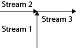
A figure shows stream 1 from the bottom and stream 2 from the left point to a point, from where stream 3 points further to the right.

Figure E19.1 Physical Situation in Example 19.1

Determine the volumetric and mass flowrates of Stream 3.
Determine the velocities in Streams 1 and 2.
If the velocity is not to exceed 1 m/s in Stream 3, determine the minimum possible pipe diameter.
Determine the superficial mass velocity Stream 3 using the pipe diameter calculated in Part (c).

Solution

Since the density is constant, the volumetric flowrate of Stream 3 is the sum of the volumetric flowrates of Streams 1 and 2, 0.015 m³/s. To obtain the mass flowrate, $\dot{m} = ρ {\dot{v}}_{3}$ , so ${\dot{m}}_{3} = (887 kg / m^{3}) (0.0 {15 m}^{3} / s) = 13 . 3 kg / s$ . Alternatively, the mass flowrate of Streams 1 and 2 could be calculated and added to get the same result.
From Equation (19.3), at constant density $u = \dot{v} / A$ . Therefore,

$\begin{matrix} u_{1} = \frac{{\dot{v}}_{1}}{A_{1}} = \frac{4 {\dot{v}}_{1}}{π D_{1}^{2}} = \frac{4 (0.006 m^{3} / s)}{π {(0.078 m)}^{2}} = 1.26 m/s & (E19.1a) \end{matrix}$

$\begin{matrix} u_{2} = \frac{{\dot{v}}_{2}}{A_{2}} = \frac{4 {\dot{v}}_{2}}{π D_{2}^{2}} = \frac{4 (0.009 m^{3} / s)}{π {(0.01 m)}^{2}} = 1.15 m/s & (E19.lb) \end{matrix}$
The diameter at which u₃ = 1 m/s can be calculated from Equation (19.3) at constant density.

$\begin{matrix} \begin{matrix} {\dot{v}}_{3} = u_{3} A_{3} \Rightarrow 0.015 m^{3} /s = (1 m/s) (\frac{π D^{2}}{4}) & ∴ D = 0.138 m \end{matrix} & (E19.1c) \end{matrix}$

If the diameter were smaller, the cross-sectional area would be smaller, and from Equation (19.3), the velocity would be larger. Hence, the result in Equation (E19.1c) is the minimum possible diameter. As shown later, actual pipes are available only in discrete sizes, so it is necessary to use the next higher pipe diameter.
From Equation (19.4), using the rounded values,

$\begin{matrix} G_{1} = \frac{{\dot{m}}_{3}}{A_{3}} = \frac{4 {\dot{m}}_{3}}{π D_{1}^{2}} = \frac{4(13.3 kg/s)}{π {(0.138 m)}^{2}} = {889.2 kg/m}^{2} /s \end{matrix} (E19.1d)$

19.1.2 Mechanical Energy Balance

The mechanical energy balance represents the conversion between different forms of energy in piping systems. With the exception of temperature changes for a gas undergoing compression or expansion with no phase change, temperature is assumed to be constant. The mechanical energy balance is

$\begin{matrix} \int_{1}^{2} \frac{dP}{ρ} + \frac{1}{2} Δ (\frac{< u^{3} >}{}) + g Δ z + e_{f} - W_{s} = 0 \end{matrix} (19.5)$

In Equation (19.5) and throughout this chapter, the difference, Δ, represents the value at Point 2 minus the value at Point 1, that is, out − in. The units in Equation (19.5) are energy/mass or length²/time². In SI units, since 1 J =1 kg m²/s², it is clear that 1 J/kg = 1 m²/s². In American Engineering units, since 1 lb_f = 32.2 ft lb_m/sec², this conversion factor (often called g_c) must be used to reconcile the units. The notation < > represents the appropriate average quantity.

The first term in Equation (19.5) is the enthalpy of the system. On the basis of the constant temperature assumption, only pressure is involved. For incompressible fluids, such as liquids, density is constant, and the term reduces to

$\begin{matrix} \int_{1}^{2} \frac{dP}{ρ} = \frac{Δ P}{ρ} \end{matrix} (19.6)$

For compressible fluids, the integral must be evaluated using an equation of state.

The second term in Equation (19.5) is the kinetic energy term. For turbulent flow, a reasonable assumption is that

$\begin{matrix} \frac{< u^{3} >}{} \approx ^{2} \end{matrix} (19.7)$

For laminar flow,

$\begin{matrix} \frac{< u^{3} >}{} \approx 2 ^{2} \end{matrix} (19.8)$

For simplicity, < u² > is hereafter represented as ², which is shortened to u².

The third term in Equation (19.5) is the potential energy term. Based on the general control volume, Δz is positive if Point 2 is at a higher elevation than Point 1.

The fourth term in Equation (19.5) is often called the energy “loss” due to friction. Of course, energy is not lost—it is just expended to overcome friction, and it manifests as a change in temperature. The procedures for calculating frictional losses are discussed later.

The last term in Equation (19.5) represents the shaft work, that is, the work done on the system (fluid) by a pump or compressor or the work done by the system on a turbine. These devices are not 100% efficient. For example, more work must be applied to the pump than is transferred to the fluid, and less work is generated by the turbine than is expended by the fluid. In this book, work is defined as positive if done on the system (pump, compressor) and negative if done by the fluid (turbine). This convention is consistent with the flow of energy in or out of the system; however, many textbooks use the reverse sign convention. Equipment such as pumps, compressors, and turbines are described in terms of their power, where power is the rate of doing work. Therefore, a device power ( ${\dot{W}}_{s}$ , energy/time) is defined as the product of the mass flowrate (mass/time) and the shaft work (energy/mass):

$\begin{matrix} {\dot{W}}_{s} = \dot{m} W_{s} \end{matrix} (19.9)$

When efficiencies are included, the last term in Equation (19.5) becomes

$\begin{matrix} η_{p} W_{s} = \frac{η_{p} {\dot{W}}_{s}}{\dot{m}} pump/compressor \end{matrix} (19.10)$

$\begin{matrix} \frac{W_{s}}{η_{t}} = \frac{{\dot{W}}_{s}}{η_{t} \dot{m}} turbine \end{matrix} (19.11)$

Example 19.2

Water in an open (source or supply) tank is pumped to a second (destination) tank at a rate of 5 lb/sec with the water level in the destination tank 25 ft above the water level in the source tank, and it is assumed that the water level does not change with the flow of water. The destination tank is under a constant 30 psig pressure. The pump efficiency is 75%. Neglect friction.

Determine the required horsepower of the pump.
Determine the pressure increase provided by the pump assuming the suction and discharge lines have the same diameter.

Solution

Turbulent flow in the pipes is assumed. The mechanical energy balance is

$\begin{matrix} \frac{Δ P}{ρ} + \frac{1}{2} Δ u^{2} + g Δ z + e_{f} - \frac{η_{p} {\dot{W}}_{s}}{\dot{m}} = 0 & (E19.2a) \end{matrix}$

Figure E19.2 is an illustration of the system.

The source tank is shown on the left and the destination tank is shown on the right, such that the destination tank is placed higher than the source tank. The water level in both tanks is labeled 1 and 2, respectively. The height difference between the two water levels is 25 feet. The pressure in the destination tank is 30 pounds per square inch gauge. The source tank points to a pump with an arrow labeled 3, and the pump points to the destination tank with an arrow labeled 4. The pump has eta subscript p equivalent to 0.75.

Figure E19.2 Physical Situation for Example 19.2

The control volume is the water in the tanks, the pipes, and the pump, and the locations of Points 1 and 2 are illustrated. The integral in the first term of Equation (19.2) is simplified to the first term in Equation (E19.2a), since the density of water is a constant. In general, the fluid velocity in tanks is assumed to be zero because tank diameters are much larger than pipe diameters, so the kinetic energy term for the liquid surface in the tank is essentially zero. Any fluid in contact with the atmosphere is at atmospheric pressure, so P₁ = 1 atm = 0 psig. The friction term is assumed to be zero in this problem, as stated. So, Equation (E19.2a) reduces to

$\begin{matrix} \frac{P_{2} - P_{1}}{ρ} + g (z_{2} - z_{1}) - \frac{η_{p} {\dot{W}}_{s}}{\dot{m}} = 0 & (E19.2b) \end{matrix}$

and

$\begin{matrix} \frac{(30 - {0) lb}_{f} {/in}^{2} {(12 in/ft)}^{2}}{{62.4 lb/ft}^{3}} + \frac{{32.2 ft/sec}^{2}}{{32.2 ft lb/lb}_{f} {/sec}^{2}} (25 - 0) ft - \frac{0.75 {\dot{W}}_{s}}{5 lb/sec} = 0 & (E19.2c) \end{matrix}$

$so, {\dot{W}}_{s} = 628 . {2 ft lb}_{f} /sec.$

Converting to horsepower yields

$\begin{matrix} {\dot{W}}_{s} = \frac{{628.2 ft lb}_{f} /sec}{{550 ft lb}_{f} /hp/sec} = 1.14 hp & (E19.2d) \end{matrix}$
To determine the pressure rise in the pump, the control volume is now taken as the fluid in the pump. So, the mechanical energy balance is written between Points 3 and 4. The mechanical energy balance reduces to

$\begin{matrix} \frac{Δ P}{ρ} - \frac{η_{p} {\dot{W}}_{s}}{\dot{m}} = 0 & (E19.2e) \end{matrix}$

The kinetic energy term is zero because the suction and discharge pipes have the same diameter. Frictional losses are assumed to be zero in this example. The potential energy term is also assumed to be zero across the pump; however, since the discharge line of a pump may be higher than the suction line, in a more detailed analysis, that potential energy difference might be included. Solving

$\begin{matrix} \frac{P ({lb}_{f} {/in}^{2}) {(12 in/ft)}^{2}}{62.4 {lb/ft}^{3}} - \frac{{0.75(628.2 ft lb}_{f} /sec)}{5 lb/sec} = 0 \end{matrix} (E19.2f)$

$gives Δ P = 40.8 {lb}_{f} {/in}^{2} .$

Example 19.3

A nozzle is a device that converts pressure into kinetic energy by forcing a fluid through a small-diameter opening. Turbines work in this way because the fluid (usually a gas) with a high kinetic energy impinges on turbine blades, causing spinning, and allowing the energy to be converted to electric power.

Consider a nozzle that forces 2 gal/min of water at 50 psia in a tube of 1-in inside diameter through a 0.1-in nozzle from which it discharges to atmosphere. Calculate the discharge velocity.

Solution

The system is illustrated in Figure E19.3. It is assumed that the velocity at a small distance from the end of the nozzle is identical to the velocity in the nozzle, but the contact with the atmosphere makes the pressure atmospheric.

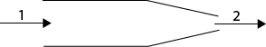
Figure E19.3 Illustration of Nozzle for Example 19.3

For the case when frictional losses may be neglected, the mechanical energy balance reduces to

$\begin{matrix} \frac{P_{2} - P_{1}}{ρ} + \frac{u_{2}^{2} - u_{1}^{2}}{2} = 0 & (E19.3a) \end{matrix}$

which yields

$\begin{matrix} \frac{(14.7 - {50) lb}_{f} {/in}^{2} {(12 in/ft)}^{2}}{{62.4 lb/ft}^{3}} + \frac{u_{2}^{2} - {[\frac{{4(2 gal/min)( ft}^{3} /7.48 gal)(min/60 sec)}{π {(1/12 ft)}^{2}}]}^{2}}{{2(32.2 ft lb/lb}_{f} {/sec}^{2})} = 0 & (E19.3b) \end{matrix}$

so u₂ = 72.4 ft/sec. For a real system, there would be some frictional losses and the actual discharge velocity would be lower than calculated here.

This problem was solved under the assumption of turbulent flow. The criterion for turbulent flow is introduced later; however, for this system, the Reynolds number is about 2 × 10⁵, which is well into the turbulent flow region.

19.1.3 Force Balance

The force balance is essentially a statement of Newton’s law. A common form for flow in pipes is

$\begin{matrix} Δ (\dot{m} \underline{u}) = \sum \underline{F} \end{matrix} (19.12)$

where F are the forces on the system. The underlined parameters indicate vectors, since there are three spatial components of a force balance. For steady-state flow and the typical forces involved in fluid flow, Equation (19.12) reduces to

$\begin{matrix} \dot{m} Δ (\underline{u}) = {\underline{F}}_{p} + {\underline{F}}_{d} + {\underline{F}}_{g} + \underline{R} \end{matrix} (19.13)$

where F_p is the pressure force on the system, F_d is the drag force on the system, F_g is the gravitational force on the system, and R is the restoring force on the system, that is, the force necessary to keep the system stationary. The term on the left side of Equation (19.12) is acceleration, confirming that Equation (19.12) is a statement of Newton’s law. The most common application of Equation (19.13) is to determine the restoring forces on an elbow. These problems are not discussed here.

19.2 Fluid Flow Equipment

The basic characteristics of fluid flow equipment are introduced in this section. The performance of pumps and compressors is dictated by their characteristic curves and, for pumps, the net positive suction head curve. The performance of these pieces of equipment is discussed in Section 19.5.

19.2.1 Pipes

Pipes and their associated fittings that are used to transport fluid through a chemical plant are usually made of metal. For noncorrosive fluids under conditions that are not of special concern, carbon steel is typical. For more extreme conditions, such as higher pressure, higher temperature, or corrosive fluids, stainless steel or other alloy steels may be needed. It may even be necessary, for very-high-temperature service such as for the flow of molten metals, to use refractory-lined pipes.

Pipes are sized using a nominal diameter and a schedule number. The higher the schedule number, the thicker the pipe walls, making pipes with a higher schedule number more suitable for higher-pressure operations. The nominal diameter is a number such as 2 in; however, there is no dimension of the pipe that is actually 2 in until the diameter reaches 14 in. For pipes with a diameter of 14 in or larger, the nominal diameter is the outside diameter. Pipes typically have integer nominal diameters; however, for smaller diameters, they can be in increments of 0.25 in. At larger diameters, the nominal diameters may only be even integer values. Table 19.1 shows the dimensions of some schedules of standard pipe.

Table 19.1 Dimensions of Standard Steel Pipe

Nominal Size (in)	Outside Diameter		Schedule Number	Wall Thickness		Inside Diameter		Inside Cross-Sectional Area
Nominal Size (in)	in	mm	Schedule Number	in	mm	in	mm	10²ft²	10⁴m²
Nominal Size (in)	Outside Diameter		Schedule Number	Wall Thickness		Inside Diameter		Inside Cross-Sectional Area
Nominal Size (in)	in	mm	Schedule Number	in	mm	in	mm	10²ft²	10⁴m²
1/8	0.405	10.29	40	0.068	1.73	0.269	6.83	0.040	0.3664
			80	0.095	2.41	0.215	5.46	0.025	0.2341
1/4	0.540	13.72	40	0.088	2.24	0.364	9.25	0.072	0.6720
			80	0.119	3.02	0.302	7.67	0.050	0.4620
3/8	0.675	17.15	40	0.091	2.31	0.493	12.52	0.133	1.231
			80	0.126	3.20	0.423	10.74	0.098	0.9059
1/2	0.840	21.34	40	0.109	2.77	0.622	15.80	0.211	1.961
			80	0.147	3.73	0.546	13.87	0.163	1.511
3/4	1.050	26.67	40	0.113	2.87	0.824	20.93	0.371	3.441
			80	0.154	3.91	0.742	18.85	0.300	2.791
1	1.315	33.40	40	0.133	3.38	1.049	26.64	0.600	5.574
			80	0.179	4.45	0.957	24.31	0.499	4.641
1 1/4	1.660	42.16	40	0.140	3.56	1.380	35.05	1.040	9.648
			80	0.191	4.85	1.278	32.46	0.891	8.275
1 1/2	1.900	48.26	40	0.145	3.68	1.610	40.89	1.414	13.13
			80	0.200	5.08	1.500	38.10	1.225	11.40
2	2.375	60.33	40	0.154	3.91	2.067	52.50	2.330	21.65
			80	0.218	5.54	1.939	49.25	2.050	19.05
2 1/2	2.875	73.03	40	0.203	5.16	2.469	62.71	3.322	30.89
			80	0.276	7.01	2.323	59.00	2.942	27.30
3	3.500	88.90	40	0.216	5.59	3.068	77.92	5.130	47.69
			80	0.300	7.62	2.900	73.66	4.587	42.61
3 1/2	4.000	101.6	40	0.226	5.74	3.548	90.12	6.870	63.79
			80	0.318	8.08	3.364	85.45	6.170	57.35
4	4.500	114.3	40	0.237	6.02	4.026	102.3	8.840	82.19
			80	0.337	8.56	3.826	97.18	7.986	74.17
5	5.563	141.3	40	0.258	6.55	5.047	128.2	13.90	129.1
			80	0.375	9.53	4.813	122.3	12.63	117.5
6	6.625	168.3	40	0.280	7.11	6.065	154.1	20.06	186.5
			80	0.432	10.97	5.761	146.3	18.10	168.1
8	8.625	219.1	40	0.322	8.18	7.981	202.7	34.74	322.7
			80	0.500	12.70	7.625	193.7	31.71	294.7
10	10.75	273.1	40	0.365	9.27	10.02	254.5	54.75	508.6
			80	0.594	15.09	9.562	242.8	49.87	463.3
12	12.75	304.8	40	0.406	10.31	11.94	303.3	77.73	722.1
			80	0.688	17.48	11.37	288.8	70.56	655.5
14	14	355.6	40	0.438	11.13	13.12	333.2	93.97	873.0
			80	0.750	19.05	12.50	317.5	85.22	791.7
16	16	406.4	40	0.500	12.70	15.00	381.0	122.7	1140
			80	0.844	21.44	14.31	363.5	111.7	1038
18	18	457.2	40	0.562	14.27	16.88	428.8	155.3	1443
			80	0.938	23.83	16.12	409.4	141.8	1317
20	20	508.0	40	0.597	15.16	18.81	477.8	193.0	1793
			80	1.031	26.19	17.94	455.7	175.5	1630
24	24	635.0	40	0.688	17.48	22.62	574.5	279.2	2594
			80	1.219	30.96	21.56	547.6	253.6	2356
Source: Adapted from Geankoplis, C., Transport Processes and Separation Process Principles, 4th ed., Prentice Hall, Upper Saddle River, 2003 [1]; Perry, R. H., and D. Green, Perry’s Chemical Engineers’ Handbook, 6th ed., McGraw-Hill, New York, 1984, Section 5 [2].

Tubing is commonly used in heat exchangers. The dimensions and use of tubing are discussed in Chapter 20.

Pipes are typically connected by screw threads, flanges, or welds. Welds and flanges are more suitable for larger diameters and higher-pressure operation. Proper welds are stronger and do not leak, whereas screwed or flanged connections can leak, especially at higher pressures. Changes in direction are usually accomplished by elbows or tees, and those changes in direction are usually 90°.

19.2.2 Valves

Valves are found in piping systems. Valves are about the only way to regulate anything in a chemical process. Valves serve several functions. They are used to regulate flowrate, reduce pressure by adding resistance, or isolate (turn flow on/off) equipment.

Two common types of valves are gate valves and globe valves. Figure 19.3 shows illustrations of several common types of valves.

Figures show the cross-sectioned structures of gate, globe, and swing check valves.

Figure 19.3 Common Types of Valves: (a) Gate, (b) Globe, (c) Swing Check (Reproduced by Permission from Couper, J. R. et al. Chemical Process Equipment: Selection and Design, 3rd ed. [New York, Elsevier, 2012] [3])

Gate valves are used for on/off control of fluid flow. The flow path through a gate valve is roughly straight, so when the valve is fully open, the pressure drop is very small. However, gate valves are not suitable for flowrate regulation because the flowrate does not change much until the “gate” is almost closed. There are also ball valves, in which a quarter turn opens a flow channel, and they can also be used for on/off regulation.

Globe valves are more suitable than gate valves for flowrate and pressure regulation. Because the flow path is not straight, globe valves have a higher pressure drop even when wide open. Globe valves are well suited for flowrate regulation because the flowrate is responsive to valve position. In a control system, the valve stem is raised or lowered pneumatically (by instrument air) or via an electric motor in response to a measured parameter, such as a flowrate. Pneumatic systems can be designed for the valve to fail open or closed, the choice depending on the service. Failure is defined as loss of instrument air pressure. For example, for a valve controlling the flowrate of a fluid removing heat from a reactor with a highly exothermic reaction, the valve would be designed to fail open so that the reactor cooling is not lost.

Check valves, such as the swing check valve, are used to ensure unidirectional flow. In Figure 19.3(c), if the flow is left to right, the swing is opened and flow proceeds. If the flow is right to left, the swing closes, and there is no flow in that direction. Such valves are often placed on the discharge side of pumps to ensure that there is no flow reversal through the pump.

19.2.3 Pumps

Pumps are used to transport liquids, and pumps can be damaged by the presence of vapor, a phenomenon discussed in Section 19.5.2. The two major classifications for pumps are positive displacement and centrifugal. For a more detailed summary of all types of pumps, see Couper et al. [3] or Green and Perry [4].

Positive-displacement pumps are often called constant-volume pumps because a fixed amount of liquid is taken into a chamber at a low pressure and pushed out of the chamber at a high pressure. The chamber has a fixed volume, hence the name. An example of a positive-displacement pump is a reciprocating pump, illustrated in Figure 19.4(a). Specifically, this is an example of a piston pump in which the piston moves in one direction to pull liquid into the chamber and then moves in the opposite direction to discharge liquid out of the chamber at a higher pressure. There are other variations of positive-displacement pumps, such as rotary pumps in which the chamber moves between the inlet and discharge points. In general, positive-displacement pumps can increase pressure more than centrifugal pumps and run at higher pressures overall. These characteristics define their applicability. Efficiencies tend to be between 50% and 80%. Positive-displacement pumps are preferred for higher pressures, higher viscosities, and anticipated viscosity variations.

Figures show the inner workings of the positive-displacement pump and the centrifugal pump.

Figure 19.4 (a) Inner Workings of Positive-Displacement Pump, (b) Inner Workings of Centrifugal Pump ([a] Reproduced by Permission from McCabe, W. L. et al., Unit Operations of Chemical Engineering, 5th ed. [New York, McGraw−Hill, 1993] [5]; [b] Reproduced by Permission from Couper, J. R. et al., Chemical Process Equipment: Selection and Design, 3rd ed. [New York, Elsevier, 2012] [3])

In centrifugal pumps, which are a common workhorse in the chemical industry, the pressure is increased by the centrifugal action of an impeller. An impeller is a rotating shaft with blades, and it might be tempting to call it a propeller because an impeller resembles a propeller. (While there might be a resemblance, the term propeller is reserved for rotating shafts with blades that move an object, such as a boat or airplane.) The blades of an impeller have small openings, known as vanes, that increase the kinetic energy of the liquid. The liquid is then discharged through a volute in which the kinetic energy is converted into pressure. Figure 19.4(b) shows a centrifugal pump. Centrifugal pumps often come with impellers of different diameters, which enable pumps to be used for different services (different pressure increases). Of course, shutdown is required to change the impeller. Although standard centrifugal pump impellers only spin at a constant rate, variable-speed centrifugal pumps also are available.

Centrifugal pumps can handle a wide range of capacities and pressures, and depending on the exact type of pump, the efficiencies can range from 20% to 90%.

19.2.4 Compressors

Devices that increase the pressure of gases fall into three categories: fans, blowers, and compressors. Figure 19.5 illustrates some of this equipment. For a more detailed summary of all types of pumps, see Couper et al. [3] or Green and Perry [4].

Figures show the inner working of the centrifugal, axial, and positive displacement compressors.

Figure a shows the Centrifugal Compressor, which has Bearings on either side. The Shaft Inlet Edge of vane and Shaft Sheave Labyrinths, along with A and B bearings holding them up. There are spiral tubes that run above and below the shafts. The following are present in the tubes below: Inlet, Eye of Impeller, Drains, Equalizing Connection, and Discharge. Arrows are shown through the spiral tubes from the Inlet. The following are present in the tubes above from the left: Bouncing Piston, Return Guide Vanes, Diffuse vane, Shaft Nut, and the First, Second and Third Stage Impellers. The Carbon Rings and Kingsbury Thrust Bearing are present on the right and left of the Bearings, respectively. Figure b shows the Axial Compressor, which has an Inlet, Stator blades, and Rotor blades. Figure c shows the Positive Displacement Compressor, which has an Inlet and a Discharge vertical tube that is enclosed by Cooling water jockets, Check valves, and a Stuffing box. A Flywheel is attached to the Stuffing box.

Figure 19.5 Inner Working of Compressors: (a) Centrifugal, (b) Axial, (c) Positive Displacement ([a] and [b] Reproduced by Permission from Couper, J. R. et al., Chemical Process Equipment: Selection and Design, 3rd ed. [New York: Elsevier, 2012]; [c] Reproduced by Permission from McCabe, W. L. et al., Unit Operations of Chemical Engineering, 5th ed. [New York: McGraw−Hill, 1993])

Fans provide very low-pressure increases (<1 psi [7 kPa]) for low volumes and are typically used to move air. Blowers are essentially mini-compressors, providing a maximum pressure of about 30 psi (200 kPa). Blowers can be either positive displacement or centrifugal, and while their general construction is similar to pumps, there are many internal differences. Compressors, which can also be either positive displacement or centrifugal, can provide outlet pressures of 1500 psi (10 MPa) and sometimes even 10 times that much.

In a centrifugal compressor, the impeller may spin at tens of thousands of revolutions per minute. If liquid droplets or solid particles are present in the gas, they hit the impeller blades at such high relative velocity that the impeller blades will erode rapidly and may cause bearings to become damaged, leading to mechanical failure. The compressor casing also may crack. Therefore, it is important to ensure that the gas in a centrifugal compressor does not contain solids and liquids. A filter can be used to keep particles out of a compressor, and a packed-bed adsorbent can also be used, for example, to remove water vapor from inlet air. Knockout drums are often provided between compressor stages with intercooling to allow the disengagement of any condensed drops of liquid and are covered in more detail in Chapter 23, Section 23.2. The seals on compressors are temperature sensitive, so a maximum temperature in one stage of a compressor is generally not exceeded, which is another reason for staged, intercooled compressor systems. It should also be noted that compressors are often large and expensive pieces of equipment that often have a large number of auxiliary systems associated with them. The coverage given in this text is very simplified but allows the estimate of the power required.

Positive-displacement compressors typically handle lower flowrates but can produce higher pressures compared to centrifugal compressors. Efficiencies for both types of compressor tend to be high, above 75%.

19.3 Frictional Pipe Flow

19.3.1 Calculating Frictional Losses

The fourth term in Equation (19.5) must be evaluated to include friction in the mechanical energy balance. There are different expressions for this term depending on the type of flow and the system involved. In general, the friction term is

$\begin{matrix} e_{f} = \frac{2 f L u^{2}}{D} = \frac{32 fL {\dot{v}}^{2}}{π^{2} D^{5}} \end{matrix} (19.14)$

where L is the pipe length, D is the pipe diameter, and f is the Fanning friction factor. (The Fanning friction factor is typically used by chemical engineers. There is also the Moody friction factor, which is four times the Fanning friction factor. Care must be used when obtaining friction factor values from different sources. It is even more confusing, since the plot of friction factor versus Reynolds number is called a Moody plot for both friction factors.) The friction factor is a function of the Reynolds number (Re = Du ρ/μ, where μ is the fluid viscosity), and its form depends on the flow regime (laminar or turbulent), and for turbulent flow, f is also a function of the pipe roughness factor (e, a length that represents small asperities on the pipe wall; values are given at the top of Figure 19.6), which is a tabulated value. Historically, the friction factor was measured and the data were plotted in graphical form. Figure 19.6 is such a plot. A key observation from Figure 19.6 is that, with the exception of smooth pipes, the friction factor asymptotically approaches a constant value above a Reynolds number of approximately 10⁵. This is called fully developed turbulent flow, and the friction factor becomes constant and can be used to simplify certain calculations, examples of which are presented later. Typical values for the pipe roughness for some common materials are shown at the top of Figure 19.6.

A line graph shows the Moody Plot for Fanning Friction Factor in Pipes.

A table at the top shows the Typical Roughness and their corresponding e Values in millimeters and inches as follows, row-wise: Cast Iron, 0.25, 0.001; Commercial Steel, 0.046, 0.0018; Drawn Tubing, 0.0015, 0.00006; Wrought Iron, 0.045, 0.0018; Galvanized Iron, 0.15, 0.0059; and Plastic, 0, 0. The graph has the horizontal axis labeled Reynolds Number, R e, ranging from 100 to 10 to the power of 8, and the vertical axis labeled Friction Factor, f, ranging from 0.001 to 0.1, both in increments of the powers of 10. A line slopes down from (250, 0.1) to (10 to the power 3, 0.01). Thirteen curves originate at points along a straight vertical line between 10 to the powers of 3 and 4, along the horizontal axis, and between 0.01 and 0.03 along the vertical axis. All curves decline at various measures and reach different points along the same vertical line from 10 to the power of 8, between 0.001 and 0.03 along the vertical axis. The curves are labeled according to the Relative Roughness eID as follows, from the top: 0.05, 0.02, 0.01, 0.005, 0.002, 0.001, 0.0005, 0.0002, 0.0001, 0.00005, 0.00002, 0.00001, and Smooth. All coordinate plots are approximate.

Figure 19.6 Moody Plot for the Fanning Friction Factor in Pipes

The friction factor for laminar flow is a theoretical result derivable from the Hagen-Poiseuille equation [6] and is valid for Re < 2100.

$\begin{matrix} f = \frac{16}{Re} = \frac{16 μ}{Duρ} \end{matrix} (19.15)$

For turbulent flow, the data have been fit to equations. One such equation is the Pavlov equation ([7] [cited in Levenspiel [8]]):

$\begin{matrix} \frac{1}{f^{0.5}} = - {4 log}_{10} [\frac{e}{3.7 D} + {(\frac{6.81}{Re})}^{0.9}] \end{matrix} (19.16)$

The Pavlov equation provides results within a few percent of the measured data. There are more accurate equations; however, they are not explicit in the friction factor. Any of these curve fits provides significantly more accuracy than reading a graph.

For flow in pipes containing valves, elbows, and other pipe fittings, there are two common methods for including the additional frictional losses created by this equipment. One is the equivalent length method, whereby additional pipe length is added to the value of L in Equation (19.14). The other method is the velocity head method, in which a value (K_i) is assigned to each valve, fitting, and so on, and an additional frictional loss term is added to the frictional loss term in Equation (19.14). These terms are of the form

$\begin{matrix} \underset{i}{Σ} \frac{K_{i} {u_{i}}^{2}}{2} \end{matrix} (19.17)$

where the index i indicates a sum over all valves, elbows, and similar components in the system. If there are different pipe diameters within the system, the velocity in Equation (19.17) is specific to each section of pipe, and a term for each section of pipe must be included. It should be noted that the equivalent K_i value for straight pipe (K_pipe) is given by

$\begin{matrix} K_{pipe} = \frac{4 fL}{D} \end{matrix} (19.18)$

Tables 19.2 and 19.3 show equivalent lengths and K_i values for some common items found in pipe networks, for turbulent flow and for laminar flow, respectively. The values are different for laminar and turbulent flow. Darby [9] presents analytical expressions for the K values that can be used for more exact calculations.

Table 19.2 Frictional Losses for Turbulent Flow

Type of Fitting or Valve	Frictional Loss, Number of Velocity Heads, K_f	Frictional Loss, Equivalent Length of Straight Pipe, in Pipe Diameters, L _eq /D
45° elbow	0.35	17
90° elbow	0.75	35
Tee	1	50
Return bend	1.5	75
Coupling	0.04	2
Union	0.04	2
Gate valve, wide open	0.17	9
Gate valve, half open	4.5	225
Globe valve, wide open	6.0	300
Globe valve, half open	9.5	475
Angle valve, wide open	2.0	100
Check valve, ball	70.0	3500
Check valve, swing	2.0	100
Contraction	0.55(1 – A₂/A₁)	27.5(1 – A₂/A₁)
Contraction A₂ << A₁	0.55	27.5
Expansion	(1 – A₁/A₂)²	50(1 – A₁/A₂)²
Expansion A₁ << A₂	1	50
Source: From Geankoplis, C., Transport Processes and Separation Process Principles, 4th ed., (Upper Saddle River, NJ: Prentice Hall, 2003); Perry, R. H., and D. Green, Perry’s Chemical Engineers’ Handbook, 6th ed. (New York: McGraw-Hill, 1984), Section 5.

Table 19.3 Frictional Loss for Laminar Flow

Frictional Loss, Number of Velocity Heads, K_f
Reynolds number	50	100	200	400	1000	Turbulent
90° elbow	17	7	2.5	1.2	0.85	0.75
Tee	9	4.8	3.0	2.0	1.4	1.0
Globe valve	28	22	17	14	10	6.0
Check valve, swing	55	17	9	5.8	3.2	2.0
Source: From Geankoplis, C., Transport Processes and Separation Process Principles, 4th ed. (Upper Saddle River, NJ: Prentice Hall, 2003), 99–100, citing Kittredge, C. P., and D. S. Rowley, “Resistance Coefficients for Laminar and Turbulent Flow Through One-Half-Inch Valves and Fittings,” Trans. ASME, 79 (1957): 1759–1766.

Another common situation involves frictional loss in a packed bed, that is, a vessel packed with solids. One application is if the solids are catalysts, making the packed bed a reactor. The frictional loss term for packed beds is obtained from the Ergun equation, which yields a friction term for a packed bed as

$\begin{matrix} e_{f} = \frac{{L u}_{s}^{2} (1 - ε)}{ε^{3} D_{p}} [\frac{150 (1 - ε) μ}{D_{p} u_{s} ρ} + 1.75] \end{matrix} (19.19)$

where u_s is the superficial velocity (based on pipe diameter, not particle diameter), D_p is the particle diameter (assumed spherical here; corrections are available for nonspherical shape), and ε is the packing void fraction, which is the volume fraction in the packed bed not occupied by solids. When Equation (19.19) is used in the mechanical energy balance, one unknown parameter, such as velocity, pressure drop, or particle diameter, can be obtained.

For incompressible flow in packed beds, the Ergun equation, Equation (19.19), is used for the friction term in the mechanical energy balance.

For the expansion and contraction losses, A_i is the cross-sectional area of the pipe, subscript 1 is the upstream area, and subscript 2 is the downstream area.

19.3.2 Incompressible Flow

19.3.2.1 Single-Pipe Systems

Incompressible flow problems fall into three categories:

Any parameter unknown in the mechanical energy balance other than velocity (flowrate) or diameter
Unknown velocity (flowrate)
Unknown diameter

For turbulent flow problems with any unknown other than velocity (or flowrate) or diameter, in the mechanical energy balance, Equation (19.5), there is a second unknown: the friction factor. The friction factor can be calculated from Equation (19.15). The solution method can use a sequential calculation, solving Equation (19.5) for the unknown once the friction factor is calculated. If there are valves, elbows, and so on, the length term in Equation (19.15) can be adjusted appropriately or Equation (19.17) can be used. Alternatively, Equations (19.14) and (19.16) can be solved simultaneously to yield all the unknowns. Example 19.5 shows both of these calculation methods. For laminar flow problems, Equation (19.15) can be combined with Equation (19.14) in the mechanical energy balance to solve any problem analytically.

For turbulent flow, if the velocity is unknown, Equations (19.5) and (19.15) must be solved simultaneously for the velocity or flowrate and the friction factor. When solving for a velocity directly, if the pump work term must be included, it is necessary to express the mass flowrate in terms of velocity. If solving for the volumetric flowrate, the second equality in Equation (19.13) must be used, and if a kinetic energy term is required in the mechanical energy balance, the velocities must be expressed in terms of volumetric flowrate. In the friction factor equation, the Reynolds number also needs to be expressed in terms of the volumetric flowrate as follows:

$\begin{matrix} Re = \frac{Duρ}{μ} = \frac{Dρ}{μ} \frac{\dot{v}}{A} = \frac{Dρ}{μ} \frac{4 \dot{v}}{π D^{2}} = \frac{4 \dot{v} ρ}{π Dμ} \end{matrix} (19.20)$

For laminar flow, an analytical solution is possible simply by using Equation (19.14) for the friction factor in the mechanical energy balance.

For turbulent flow, if the diameter is unknown, Equations (19.5) and (19.13) (second equality involving flowrate and diameter to the fifth power) must be solved simultaneously, using Equation (19.20) for the Reynolds number. For laminar flow, an analytical solution may once again be possible by using Equation (19.12) for the friction factor in the mechanical energy balance. If kinetic energy terms are involved, an unknown diameter will appear when expressing velocity in terms of flowrate. If minor losses are involved, the equivalent length will include a diameter term, and the K-value method will include a diameter in the conversion between flowrate and velocity.

Examples 19.4 and 19.5 illustrate the methods for solving these types of problems.

Example 19.4

Consider a physical situation similar to that in Example 19.2. The flowrate between tanks is 10 lb/sec. The source-tank level is 10 ft off of the ground, and the discharge-tank level is 50 ft off of the ground. For this example, both tanks are open to the atmosphere. The suction-side pipe is 2-in, schedule-40, commercial steel, and the discharge-side pipe is 1.5-in, schedule-40, commercial steel. The length of the suction line is 25 ft, and the length of the discharge line is 60 ft. The pump efficiency is 75%. Losses due to fittings, expansions, and contractions may be assumed negligible for this problem.

Determine the required horsepower of the pump.
Determine the pressures before and after the pump.

Solution

The physical situation is depicted in Figure E19.4.

The source tank is shown on the left and the destination tank is shown on the right, such that the destination tank is placed higher than the source tank. The water level in both tanks is labeled 1 and 2, respectively. The height difference between the two water levels is 25 feet. The source tank points to a pump with an arrow labeled 3, and the pump points to the destination tank with an arrow labeled 4. The pump is placed much below the source tank and has eta subscript p equivalent to 0.75. The distance between the water levels in the two tanks to the base of the pump is 10 and 50 feet, respectively.

Figure E19.4

For the control volume of the fluid in both tanks, the pipes, and the pump, the mechanical energy balance reduces to

$\begin{matrix} g Δ z + e_{f, suct} + e_{f, disch} - \frac{η_{p} {\dot{W}}_{s}}{\dot{m}} = 0 & (E19.4a) \end{matrix}$

The pressure term is zero, because both tanks are open to the atmosphere (P₁ = P₂ = 1 atm). The kinetic energy term is zero, because the velocities of the fluid at the surfaces of both tanks are assumed to be zero. There are two friction terms, one for the suction side of the pump and one for the discharge side of the pump, because the friction factors are different due to the different pipe diameters.

To calculate the friction terms, the Reynolds numbers must be calculated first for each section to determine whether the flow is laminar or turbulent. Since a temperature is not provided, the density is assumed to be 62.4 lb/ft³, and the viscosity is assumed to be 1 cP = 6.72 ×10^–4 lb/ft/sec. Using Table 19.1 for the schedule pipe diameter and cross-sectional area, the Reynolds number for the suction side is

$\begin{matrix} Re = \frac{Duρ}{μ} = \frac{(2.067/12 ft) (\frac{10 lb/sec}{({0.0233 ft}^{2}) ({62.4 lb/ft}^{3})}) ({62.4 lb/ft}^{3})}{6.72 \times 10^{- 4} lb/ft/sec} = 110,000 & (E19.4b) \end{matrix}$

Similarly, the Reynolds number for the discharge side is 141,200. Therefore, the flow is turbulent in both sections of pipe. The friction factor is now calculated for each section of pipe. For the suction side, with commercial-steel pipe (e = 0.0018 in from the top of Figure 19.6),

$\begin{matrix} \frac{1}{f^{0.5}} = - {4 log}_{10} [\frac{0.0018 in}{3.7(2.067 in)} + {(\frac{6.81}{110,010})}^{0.9}] & (E19.4c) \end{matrix}$

so f_suct = 0.0054. Similarly, f_iisch = 0.0055. Now, the mechanical energy balance on the entire system is used to solve for the pump power:

$\begin{matrix} \begin{array}{l} \frac{{(32.2 ft/sec}^{2})(40 ft)}{{32.2 ft lb/lb}_{f} {/sec}^{2}} + \frac{2(0.0054)(25 ft) {(\frac{10 lb/sec}{({0.0233 ft}^{2}) ({62.4 lb/ft}^{3})})}^{2}}{(\frac{2.067}{12} ft) ({32.2 ft lb/lb}_{f} {/sec}^{2})} \\ + \frac{2(0.0055)(60 ft) {(\frac{10 lb/sec}{({0.01414 ft}^{2}) ({62.4 lb/ft}^{3})})}^{2}}{(\frac{1.61}{12} ft) ({32.2 ft lb/lb}_{f} {/sec}^{2})} - \frac{(0.75) {\dot{W}}_{s} {(550 ft lb}_{f} /sec/hp)}{(10 lb/sec)} = 0 \end{array} \end{matrix} (E19.4d)$

Solving Equation (E19.4d) gives ${\dot{W}}_{s} = 1 . 5 hp$ . If the contribution of each term is enumerated, 0.97 hp is to overcome the potential energy and 0.48 hp is to overcome the discharge line friction, with 0.056 hp to overcome the suction line friction. Generally, potential energy differences and pressure differences are more significant than frictional losses.
To obtain the pressure on the suction side of the pump, the mechanical energy balance is written on the control volume of the fluid in the tank and pipes before the pump.

$\begin{matrix} \frac{P_{3} - P_{1}}{ρ} + \frac{u_{3}^{2}}{2} + g Δ z + e_{f} = 0 \end{matrix} (E19.4e)$

$\begin{matrix} \begin{array}{l} \frac{[P_{3} - (14.7)] {(144)lb}_{f} {/ft}^{2}}{{62.4 lb/ft}^{3}} + \frac{{(\frac{10 lb/sec}{({0.0233 ft}^{2}) ({62.4 lb/ft}^{3})})}^{2}}{{2(32.2 ft lb/lb}_{f} {/sec}^{2})} + \frac{{(32.2 ft/sec}^{2})(- 10 ft)}{{32.2 ft lb/lb}_{f} {/sec}^{2}} \\ + \frac{2(0.0054)(15 ft) {(\frac{10 lb/sec}{({0.0233 ft}^{2}) ({62.4 lb/ft}^{3})})}^{2}}{(\frac{2.067}{12} ft) {(32.2 ft lb/lb}_{f} {/sec}^{2})} = 0 \end{array} \end{matrix} (E19.4f)$

So, P₃ = 17.7 psi. It is observed that the height change in the potential energy term is negative, since the point at the pump entrance is below the liquid level in the tank, noting that the z-coordinate system is positive in the upward direction.

There are two ways to obtain the discharge-side pressure. One is to solve the mechanical energy balance on the control volume between Points 4 and 2. The other method is to write the mechanical energy balance on the fluid in the pump (pressure, kinetic energy, and work terms) to obtain the pressure rise in the pump. Both methods give the same result of P₄ = 28.9 psi.

The discharge line of a pump is at a slightly higher elevation than the suction line, as illustrated. This height difference is small and is neglected in this analysis.

Example 19.5

Determine the required horsepower of the pump in Example 19.4 if the presence of one 90° elbow and one wide-open gate valve in the suction line and one wide-open gate valve, one half-open globe valve, and two 90° elbows in the discharge line are included.

Solution

The solution to this problem starts with Equation (E19.4d). Friction terms must be added for each item in each section of pipe. Using the equivalent length method for the suction line, L_eq = 25 ft + (2.067/12 ft) (35 + 9 + 27.5) = 37.3 ft, where the equivalent length terms for the elbow, gate valve, and contraction upon leaving the source tank, respectively, are obtained from Table 19.2. For the discharge line, L_q = 60 ft + (1.61/12 ft) [2(35) + 9 + 475 + 50] = 141.04 ft, where the equivalent length terms are for the two elbows, gate valve, globe valve, and expansion upon entering the destination tank, respectively. In terms of friction, these items add significantly to the frictional losses, especially the half-open globe valve in the discharge line. The result is that $\dot{W} s = 2 . 71 hp$ .

It is also possible to use the velocity heads method. For the suction side, once again referring to Table 19.2, S,K_i = 0.75 + 0.17 + 0.55 = 1.47, so a term of $1.47 u_{1}^{2} / 2 / 32.2$ is added to the mechanical energy balance. For the discharge side, K = 2(0.75) + 0.17 + 9.5 + 1 = 12.17, so a term of $12.17 u_{2}^{2} / 2 / 32.2$ is added to the mechanical energy balance. The result is 2.12 hp, which illustrates that the two methods do not give exactly the same results. The difference is because both methods are empirical and are subject to uncertainties. Either method is within the typical tolerance of a design specification. To provide flexibility and since pumps are typically available at fixed values, at least a 3 hp pump would probably be used here, and valves would be used to adjust the flowrate to the desired value.

Example 19.6

A fuel oil (μ = 70 × 10^-³ kg/m/s, SG = 0.9) is pumped through 2.5-in, schedule-40 pipe for 500 m at 3 kg/s. The discharge point is 5 m above the inlet, and the source and destination are both at 101 kPa. If the pump is 80% efficient, what power is required?

Solution

The situation is shown in Figure E19.6.

An arrow from the left is shown pointing to a pump at the bottom, which points right to a destination 5 meters above it. The pump has eta subscript p equivalent to 0.80.

Figure E19.6

The control volume is the fluid in the pipe between the source and destination. The mechanical energy balance contains only the potential energy, friction, and work terms, since there is only one pipe (velocity constant) and since the pressures are identical at the source and destination. The mechanical energy balance is

$\begin{matrix} g Δ z + e_{f} - \frac{η_{p} {\dot{W}}_{s}}{\dot{m}} = 0 & (E19.6a) \end{matrix}$

As in Example 19.4, the Reynolds number should be calculated first:

$\begin{matrix} Re = \frac{Duρ}{μ} = \frac{(0.06271 m) (\frac{3 kg/s}{(0.003089 m^{2}) ({900 kg/m}^{3})}) ({900 kg/m}^{3})}{70 \times 10^{- 3} kg/m/s} = 870 & (E19.6b) \end{matrix}$

Therefore, the flow is laminar, and the friction factor f = 16/Re. A hint that the flow might be laminar is that the fluid is 70 times more viscous than water. This emphasizes the need to check the Reynolds number before proceeding.

The mechanical energy balance is then

$\begin{matrix} {(9.8 m/s}^{2})(5 m) + \frac{2 (\frac{16}{870}) (500 m) {(\frac{3 kg/s}{(0.003089 m^{2} {)(900 kg/m}^{3})})}^{2}}{0.06271m} - \frac{0.8 {\dot{W}}_{s}}{3 kg/s} = 0 & (E19.6c) \end{matrix}$

which gives ${\dot{W}}_{s} = 1464 W$ .

Example 19.7

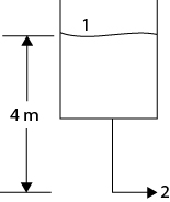
Water flows from a constant-level tank at atmospheric pressure through 8 m of 1-in, schedule-40, commercial-steel pipe. It discharges to atmosphere 4 m below the level in the source tank. Calculate the mass and volumetric flowrates, neglecting entrance and exit losses.

Solution

Since the flowrate is unknown, the velocity is unknown, so the Reynolds number cannot be calculated, which means that the friction factor cannot be calculated initially. A simultaneous solution of the friction factor equation and the mechanical energy balance is necessary. Since the fluid is water, turbulent flow will be assumed, but it must be checked once the velocity or flowrate has been calculated.

The control volume is the fluid in the tank and the discharge pipe. In Figure E19.7, Point 1 is the level in the tank, which is at zero velocity, and Point 2 is the pipe discharge to the atmosphere.

A tank filled with a fluid is shown. The level of fluid is marked 1, which is at a height of 4 meters from the base. An arrow labeled 2, points from the bottom of the tank and turns right on reaching the base.

Figure E19.7

The mechanical energy balance reduces to

$\begin{matrix} \frac{u_{2}^{2}}{2} + g Δ z + \frac{2 fL u_{2}^{2}}{D} = 0 = \frac{u_{2}^{2}}{2} = ({9.8 m/s}^{2}) (- 4 m) + \frac{2 f (8 m) u_{2}^{2}}{0.02664 m} & (E19.7a) \end{matrix}$

and the friction factor is

$\begin{matrix} \frac{1}{f^{0.5}} = - 4 \log_{10} [\frac{4.6 \times 10^{- 5} m}{3.7(0.02664 m)} + {(\frac{{6.81(10}^{- 3} kg/m/s)}{(0.02664 m)(u_{2} {)(1000 kg/m}^{3})})}^{0.9}] & (E19.7b) \end{matrix}$

Equations (E19.7a) and (E19.7b) are solved simultaneously to give f = 0.0062 and u₂ = 3.04 m/s. Using the relationships between velocity, volumetric flowrate, and mass flowrate, the results are ${\dot{v}}_{2} = 1.69 \times 10^{- 3} m^{3} / s$ and $\dot{m} = 1 . 69 kg / s$ . Now, the Reynolds number must be checked using the calculated velocity, and Re = 80,960, so the turbulent flow assumption is valid.

Example 19.8

Number 6 fuel oil (μ = 800 cP, ρ = 62 lb/ft³) flows in a 1.5-in, schedule-40 pipe over a distance of 1000 ft. The discharge point is 20 ft above the inlet, and the source and discharge are both at 1 atm. A 15 hp pump that is 75% efficient is used. What is the flowrate in the pipe?

Solution

The mechanical energy balance reduces to

$\begin{matrix} g Δ z + \frac{32 fL {\dot{v}}^{2}}{π^{2} D^{5}} - \frac{η_{p} {\dot{W}}_{s}}{ρ \dot{v}} = 0 & (E19.8a) \end{matrix}$

The friction expression is in terms of the volumetric flowrate, and in the third term, the mass flowrate in the denominator is also expressed in terms of the volumetric flowrate. The volumetric flowrate is the unknown variable. Given the high viscosity, laminar flow is assumed. This assumption must be checked once a flowrate is calculated. For laminar flow, since f = 16/Re, Equation (E19.8a) becomes

$\begin{matrix} g Δ z + \frac{32 L {\dot{v}}^{2}}{π^{2} D^{5}} \frac{16 π Dμ}{4 \dot{v} ρ} - \frac{η_{p} {\dot{W}}_{s}}{ρ \dot{v}} = 0 & (E19.8b) \end{matrix}$

where the fourth equality in Equation (19.20) is used for the Reynolds number. All terms are known other than the volumetric flowrate, so

$\begin{matrix} \begin{array}{l} {32.2 ft/sec}^{2} (20 ft)+ \frac{128(1000 ft)(800 cP)(6.72 \times 10^{- 4} lb/ft/sec/cP) \dot{v}}{π {(\frac{1.610 in}{12 in/ft})}^{4} {(62 lb/ft}^{3})} \\ - \frac{{0.75(15 hp)(550 ft lb}_{f} {/sec/hp)(32.2 ft lb/lb}_{f} {/sec}^{2})}{\dot{v} ({62 lb/ft}^{3})} = 0 \end{array} & (E19.8c) \end{matrix}$

The solution is $\dot{v} = {0.054 ft}^{3} / sec$ . Checking the Reynolds number,

$\begin{matrix} Re = \frac{4 \dot{v} ρ}{π Dμ} = \frac{{4(0.054 ft}^{3} {/sec)(62 lb/ft}^{3})}{π (\frac{1.610 in}{12 in/ft}) (800 cP) (6.72 \times 10^{- 4} lb/ft/sec/cP)} = 59.1 & (E19.8d) \end{matrix}$

so the flow is indeed laminar.

19.3.2.2 Multiple-Pipe Systems

For complex, multiple-pipe systems, including branching or mixing pipe systems, as illustrated in Figure 19.7, there are two sets of key relationships.

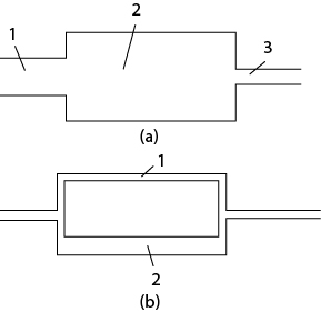
Illustrations of pipes of different diameters in series and parallel.

Figure 19.7 Multiple Pipe Systems: (a) Pipes of Different Diameters in Series, (b) Pipes of Different Diameters in Parallel

For pipes in series, the mass flowrate is constant and the pressure differences are additive:

$\begin{matrix} {\dot{m}}_{1} = {\dot{m}}_{2} = {\dot{m}}_{3} \end{matrix} (19.21)$

$\begin{matrix} Δ P = Δ P_{1} + Δ P_{2} + Δ P_{3} \end{matrix} (19.22)$

For pipes in parallel, the mass flowrates are additive and the pressure differences are equal:

$\begin{matrix} \dot{m} = {\dot{m}}_{1} + {\dot{m}}_{2} = {\dot{m}}_{3} \end{matrix} (19.23)$

$\begin{matrix} Δ P_{1} = Δ P_{2} = Δ P_{3} \end{matrix} (19.24)$

Equation (19.21) is just the mass balance; the mass flowrate through each section must be constant. Equation (19.22) just means that the pressure drops in all sections in series are additive.

In the case of parallel flow, Equation (19.23) means that the mass flowrates in and out of the parallel section are additive, since mass must be conserved. Equation (19.24) means that the pressure drops in parallel sections are equal. This is because mixing streams must be designed to be at the same pressure, or the flowrates will readjust so the pressures at the mixing point are identical. This concept is discussed in more detail later.

The solution method is to write all of the relevant equations, including the mechanical energy balance, friction factor expression, and mass balance, along with the appropriate constraints from Equations (19.21) through (19.24), and solve the equations simultaneously. It is understood that this method applies to any number of pipes in series or parallel.

Example 19.9

Water flows through a pipe, splits into two parallel pipes, and then the fluids mix into another single pipe, as in Figure 19.7(b). All piping is commercial steel. The equivalent length of Branch 1 is 75 m, and the equivalent length of Branch 2 is 50 m. The elevation at the split point is the same as the elevation at the mixing point. Branch 1 is 2-in, schedule-40 pipe, and Branch 2 is 1.5-in, schedule-40 pipe. The pressure drop across Branch 1 is fixed at 100 kPa. Determine the volumetric flowrate in each branch and the total volumetric flowrate. What information could be obtained if the pressure drop was not provided?

Solution

The mechanical energy balance for both sections reduces to

$\begin{matrix} \frac{Δ P_{i}}{ρ} + \frac{2 f_{i} L_{i} u_{i}^{2}}{D_{i}} = 0 & (E19.9a) \end{matrix}$

where the subscript i denotes a parallel section of pipe. The kinetic energy terms are not present in Equation (E19.9a) because the control volume is the parallel pipes not including the feed pipe, the mixing point, the split point, and the discharge pipe. There are four unknowns, the friction factor and velocity in each section. The mechanical energy balance for each section is Equation (E19.9a), and there are two expressions for the friction factor, so the problem can be solved. Because the two branches are in parallel and then mix, the pressure drop in each section is the same, as shown in Equation (19.24), and it is negative, since the downstream pressure is less than the upstream pressure. Initially, turbulent flow will be assumed. The equations are

$\begin{matrix} \frac{- 100,000 Pa}{{1000 kg/m}^{3}} + \frac{2 f_{1} (75 m) u_{1}^{2}}{0.0525m} = 0 & (E19.9b) \end{matrix}$

$\begin{matrix} \frac{- 100,000 Pa}{{1000 kg/m}^{3}} + \frac{2 f_{2} (50 m) u_{2}^{2}}{0.04089 m} = 0 & (E19.9c) \end{matrix}$

$\begin{matrix} \frac{1}{f_{1}^{0.5}} = - 4 \log_{10} [\frac{4.6 \times 10^{- 5} m}{3.7(0.0525 m)} + {(\frac{{6.81(10}^{- 3} kg/m/s)}{(0.0525 m)(u_{1} {)(1000 kg/m}^{3})})}^{0.9}] & (E19.9d) \end{matrix}$

$\begin{matrix} \frac{1}{f_{2}^{0.5}} = - 4 \log_{10} [\frac{4.6 \times 10^{- 5} m}{3.7(0.04089 m)} + {(\frac{{6.81(10}^{- 3} kg/m/s)}{(0.04089 m)(u_{1} {)(1000 kg/m}^{3})})}^{0.9}] & (E19.9e) \end{matrix}$

Solving Equations (E19.9b) to (E19.9e) simultaneously gives f₁ = 0.0053, u₁ = 2.57 m/s, f₂ = 0.0056, u₂ = 2.69 m/s. The volumetric flowrates are ${\dot{v}}_{1} = 0.00 {56 m}^{3} / s$ and ${\dot{v}}_{2} = 0.00 {35 m}^{3} / s$ . While Branch 2 is shorter, the smaller diameter has a stronger effect on the friction, as seen by the fifth-power dependence in Equation (19.14), so Branch 2 has a smaller flowrate.

Finally, the Reynolds numbers must be calculated to prove that the flow is turbulent. The results are Re₁ = 134,700, and Re₂ = 110,160, so the flow is indeed turbulent.

When streams mix, the pressure will be the same. If a pipe system is designed such that the pressures at a mixing point are not the same, the flowrates will adjust (as illustrated in Example 19.9) to make the mixing-point pressures identical, and the flowrates will not be as designed. This is important because steady-state process simulators allow streams to be mixed at different pressures, and the lowest pressure is taken as the outlet pressure unless an outlet pressure or a mixing-point pressure drop is specified. Just because steady-state process simulators allow this to be done does not make it physically correct. Valves are used to reduce higher pressures to make the pressures equal at a mixing point. When using simulators, it is the user’s responsibility to include appropriate devices to make the simulation correspond to reality.

19.3.3 Compressible Flow

For compressible flow, the integral in the mechanical energy balance in Equation (19.5) must be evaluated, since the density is not constant. There are two limiting cases for frictional flow through a pipe section: isothermal flow and adiabatic flow. For isothermal flow of an ideal gas, the density is expressed as

$\begin{matrix} ρ = \frac{PM}{RT} \end{matrix} (19.25)$

where M is the molecular weight, and the integral can be evaluated. For adiabatic, reversible flow of an ideal gas, the temperature in Equation (19.25) is expressed in terms of pressure to evaluate the integral in Equation (19.5) using a relationship obtained from thermodynamics:

$\begin{matrix} T = T_{1} {(\frac{P}{P_{1}})}^{\frac{γ - 1}{γ}} \end{matrix} (19.26)$

where

$\begin{matrix} γ = \frac{C_{p}}{C_{v}} \end{matrix} (19.27)$

where C_p and C_v are the constant pressure and constant volume heat capacities, respectively. The results are expressed in terms of the superficial mass velocity, G. For isothermal, turbulent flow, the result, presented without derivation, is

$\begin{matrix} \frac{M}{2 RT} (P_{2}^{2} - P_{1}^{2}) + G^{2} \ln (\frac{P_{1}}{P_{2}}) + \frac{2 f L_{eq} G^{2}}{D} = 0 \end{matrix} (19.28)$

which can be solved for an unknown pressure, superficial mass velocity (G), diameter (by expressing superficial mass velocity in terms of diameter), or length. For isothermal, laminar flow, the result is

$\begin{matrix} \frac{M}{4 RT} (P_{2}^{2} - P_{1}^{2}) + G^{2} \ln (\frac{P_{1}}{P_{2}}) + \frac{16 μ L_{eq}}{D^{2}} = 0 \end{matrix} (19.29)$

Equation (19.29) is a quadratic in G, or if G is known, any other variable can be found. For adiabatic, turbulent flow, the result is

$\begin{matrix} \frac{γ}{γ + 1} \frac{M}{R T_{1}} P_{1}^{2} [1 - {(\frac{P_{2}}{P_{1}})}^{\frac{γ + 1}{γ}}] - \frac{2 f L_{eq}}{D} - \frac{1}{γ} \ln (\frac{P_{1}}{P_{2}}) = 0 \end{matrix} (19.30)$

For compressible flow in packed beds, the Ergun equation, Equation (19.19), is used for the friction term, and the pressure term in the mechanical energy balance is integrated assuming either isothermal or adiabatic flow. For isothermal flow, the result is

$\begin{matrix} \frac{M}{2 G^{2} RT} (P_{2}^{2} - P_{1}^{2}) + \frac{L (1 - ε)}{D_{p} ε^{3}} [\frac{150 μ (1 - ε)}{D_{p} u_{s} ρ} + 1.75] = 0 \end{matrix} (19.31)$

where subscript 1 is upstream and subscript 2 is downstream. Quite often, it is stated that the mechanical energy balance for packed beds, which is the Ergun equation in Equation (19.19), can be used for gases as long as the pressure drop is less than 10% of the average pressure. However, with the computational tools now available, there is really no need for that approximation.

In Equations (19.28) through (19.33), it is assumed that the flow is in a pipe; therefore, there is no work term. The potential energy term is neglected because it is generally negligible for gases due to their low density.

19.3.4 Choked Flow

In evaluating the flow of compressible fluids, there exists a limit for the maximum velocity of the fluid (gas), that is, the speed of sound in the fluid. As an example, consider a pressurized gas in a supply tank (Tank 1) that is connected to a destination tank (Tank 2) via a pipe. Initially, Tank 1 and Tank 2 are at the same pressure, so no gas flows between them. Gradually, the pressure in Tank 2 is reduced and gas starts to flow from Tank 1 to Tank 2. It seems logical that the lower the pressure in Tank 2, the higher the gas flow rate is and the higher is the velocity of gas entering Tank 2. However, at some critical pressure for Tank 2, $P_{2}^{*}$ , the flow of gas into Tank 2, reaches sonic velocity (the speed of sound). Decreasing the tank pressure below this critical pressure has no effect on the exit velocity of the gas entering Tank 2; that is, it remains constant at the speed of sound. This phenomenon of choked flow occurs because the change in downstream pressure must propagate upstream for the change in flow to occur. The speed at which this propagation occurs is the speed of sound. Thus, when the gas velocity is at the speed of sound, any further decrease in downstream pressure cannot be propagated upstream, and the flow cannot increase further. Therefore, there is a critical (maximum) superficial mass velocity of gas, G*, that can be transferred from Tank 1 to Tank 2 through the pipe. The relationships for critical flow in pipes under turbulent flow conditions are as follows:

Isothermal flow:

$\begin{matrix} G^{*} = \frac{P_{2}^{*}}{P_{1}} \sqrt{P_{1} ρ_{1}} \end{matrix} (19.32)$

and

$\begin{matrix} \frac{4 f L_{eq}}{D} = {(\frac{P_{1}}{P_{2}^{*}})}^{2} - 2 \ln (\frac{P_{1}}{P_{2}^{*}}) - 1 \end{matrix} (19.33)$

Adiabatic flow:

$\begin{matrix} G^{*} = \sqrt{γ P_{1} ρ_{1}} {(\frac{P_{2}^{*}}{P_{1}})}^{(γ + 1) / 2 γ} \end{matrix} (19.34)$

and

$\begin{matrix} \frac{4 f L_{eq}}{D} = \frac{2}{γ + 1} [{(\frac{P_{1}}{P_{2}^{*}})}^{(γ + 1) / γ} - 1] - \frac{2}{γ} \ln (\frac{P_{1}}{P_{2}^{*}}) \end{matrix} (19.35)$

When evaluating compressible flows, a check for critical flow conditions in the system should always be done. Usually, critical flow is not an issue when P₂ > 0.5P₁, but it is always a good idea to check. The use of Equations (19.32) through (19.35) is illustrated in Example 19.10.

Example 19.10

A fuel gas has an average molecular weight of 18, a viscosity of 10^-5 kg/m s, and a γ value of 1.4. It is sent to neighboring industrial users through 4-in, schedule-40, commercial-steel pipe. One such pipeline is 100 m long. The pressure at the plant exit is 1 MPa, and the required pressure at the receiver’s plant is 500 kPa. It is estimated that the gas maintains a constant temperature of 75°C over the entire length of 100 m. Estimate the volumetric flowrate of the fuel gas, metered at 1 atm and 60°C.

Solution

The conditions for critical flow should be checked first, and this requires the simultaneous solution of Equations (19.32) and (19.33) to find $P_{2}^{*}$ . An approximation can be made by assuming that the flow is fully developed turbulent and then checking this assumption. For fully developed turbulent flow, from Equation (19.16),

$\begin{matrix} \frac{1}{f^{0.5}} = - 4 \log_{10} [\frac{e}{3.7 D}] = - 4 \log_{10} [\frac{4.6 \times 10^{- 5} m}{3.7(0.0123 m)}] \Rightarrow f = 0.00408 & (E19.10a) \end{matrix}$

Substituting in Equation (19.33) gives

$\begin{matrix} \frac{4 f L_{eq}}{D} \frac{4 (0.00408)(100)}{(0.10226)} = {(\frac{P_{1}}{P_{2}^{*}})}^{2} - 2 \ln (\frac{P_{1}}{P_{2}^{*}}) - 1 & (E19.10b) \end{matrix}$

Solving gives $P_{2}^{*} = 223.9 kPa < 500 kPa$ ; therefore, the flow is not choked. The actual friction factor is within a few percent of that calculated in Equation (E19.10a), and this difference does not affect the result regarding whether the flow is choked.

Equation (19.28) can now be solved for the superficial mass velocity:

$\begin{matrix} G = {[\frac{\frac{M}{2 RT} (P_{1}^{2} - P_{2}^{2})}{\frac{2 f L_{eq}}{D} + \ln (\frac{P_{1}}{P_{2}})}]}^{0.5} & (E19.10c) \end{matrix}$

All terms in Equation (E19.10c) are given other than the friction factor, which must be calculated. So,

$\begin{matrix} G = {[\frac{\frac{18 kg/kmol}{{2(8314 m}^{3} Pa/kmol/K)(348 K)} ({(10^{6} Pa)}^{2} - {(5 \times 10^{5} Pa)}^{2})}{\frac{2 f (100 m)}{0.10226 m} + \ln (\frac{1MPa}{0.5MPa})}]}^{0.5} & (E19.10d) \end{matrix}$

The friction factor, using the e value for commercial steel at the top of Figure 19.6, is

$\begin{matrix} \frac{1}{f^{0.5}} = - 4 \log_{10} [\frac{4.6 \times 10^{- 5} m}{3.7(0.10226 m)} + {(\frac{{6.81(10}^{- 5} kg/m/s)}{(0.10226 m) G})}^{0.9}] & (E19.10e) \end{matrix}$

where the Reynolds number is expressed as DG/μ. Equations (E19.10d) and (E19.10e) can be solved simultaneously for G. A possible approximation is to assume fully turbulent flow, as was done when checking for choked flow. In that case, the Reynolds number in the Pavlov equation is assumed to be large, so the friction factor asymptotically approaches a value calculated from only the roughness term. In this case, f = 0.004077. Then, from Equation (E19.10d), G = 518.8 kg/m²s. Simultaneous solution of Equations (E19.10d) and (E19.10e) yields f = 0.00411 and G = 516.7 kg/m²s, so the fully turbulent approximation is reasonable, even though an exact solution is possible. The Reynolds number is DG/μ = 5.28 × 10⁶, which, from Figure 19.6, is in the fully turbulent, constant-friction-factor region.

Since $G = \dot{m} / A = ρ \dot{v} / A$ , using the exact solution, with the density calculated using the ideal gas law ρ = PM/RT,

$\begin{matrix} \dot{v} = \frac{{(516.7 kg/m}^{2} /s)(0.0082124 m^{2})}{(\frac{101,325 Pa(18 kg/kmol)}{8314 m^{3} Pa/kmol/K(333 K)})} = {6.44m}^{3} /s \end{matrix} (E19.10f)$

It is observed that the temperature and pressure used to calculate the density in Equation (E19.10d) are not the conditions in the pipeline, because the flowrate required is at 1 atm and 60°C. Since the density of gases is a function of temperature and pressure obtained through an equation of state, a volumetric flowrate must have temperature and pressure specified. In the gas industry, where American Engineering units are common, the standard conditions, known as standard cubic feet (SCF), are at 1 atm and 60°F.

If the second tank were at a pressure of $P_{2}^{*} = 223 . 9 kPa$ or less, then the superficial mass velocity would be at its maximum value, given by Equation (19.32) (where ρ₁ = 6.5016 kg/m³):

$G^{*} = \frac{P_{2}^{*}}{P_{1}} \sqrt{P_{1} ρ_{1}} = \frac{223,900}{10^{6}} \sqrt{(10^{6}) (6.5016)} = {570.9 kg/m}^{2} /s$

19.4 Other Flow Situations

19.4.1 Flow Past Submerged Objects

Objects moving in fluids and fluids moving past stationary, submerged objects are similar situations that are described by the force balance. When an object is released in a stationary fluid, it will either fall or rise, depending on the relative densities of the object and the fluid. The object will accelerate and reach a terminal velocity. The period of acceleration is found through an unsteady-state force balance, which is

$\begin{matrix} m \frac{du}{dt} = - (ρ_{s} - ρ) gV + F_{drag} \end{matrix} (19.36)$

where ρ_s is the object density, and ρ is the fluid density. For solid objects, the density difference most likely will be positive, so the object moves downward due to gravity and the drag force resists that motion—hence the opposite signs of the two terms on the right-hand side of Equation (19.36). However, for a gas bubble in a liquid, for example, the density difference is negative, so the bubble rises and the drag force resists that motion. Since velocity is generally defined as being positive moving away from gravity, because that is the positive direction of the coordinate system, the signs reconcile.

For a sphere, the mass is

$\begin{matrix} m = ρ_{s} V = ρ_{s} \frac{{π D}_{s}^{3}}{6} \end{matrix} (19.37)$

where D_s is the sphere diameter, and the volume is defined in Equation (19.37). The drag force on an object is defined as

$\begin{matrix} F_{drag} = C_{D} \frac{ρ u^{2}}{2} A_{proj} = C_{D} \frac{ρ u^{2}}{2} \frac{{π D}_{s}^{2}}{4} \end{matrix} (19.38)$

where C_D is a drag coefficient that may be thought of as an analog to the friction factor, A_proj is the projected area normal to the direction of flow, and u is the velocity of the object relative to the fluid. For a sphere, the projected area is that of a circle, as shown in the second equality of Equation (19.38). For a cylinder with transverse flow, this area is that of a rectangle. Equation (19.37), Equation (19.38), and the volume of a sphere may be substituted into Equation (19.36), and integration between the limits of zero velocity at time zero and velocity u at time t yields the transient velocity. The transient velocity approaches the terminal velocity at t → ∞, which can also be obtained by solving for velocity in Equation (19.36) when du/dt = 0, that is, at steady state, when the sum of the forces on the object equal zero. The terminal velocity is

$\begin{matrix} u_{t}^{2} = \frac{4 (ρ_{s} - ρ) g D_{s}}{3 C_{D} ρ} \end{matrix} (19.39)$

An expression for the drag coefficient is now needed, just as an expression for the friction factor was needed for pipe flow. Similar to pipe flow, there are different flow regimes with different drag coefficients. The Reynolds number for a sphere is defined as Re = D_su_t ρ/μ, where the density and viscosity are always that of the fluid, and if Re << 1, which is called creeping flow, this is the Stokes flow regime. Stokes’ law, which is a theoretical result, states that the drag force in Equation (19.36) is defined as

$\begin{matrix} F_{d} = 3 π µ D_{s} u_{t} \end{matrix} (19.40)$

which yields

$\begin{matrix} C_{D} = \frac{24}{Re} \end{matrix} (19.41)$

Stokes’ law must be applied only when it is valid, even though its use makes the mathematical results much simpler. In addition to the Reynolds number constraint, the assumptions involved in Stokes’ law are a rigid sphere and that gravity is the only body force. An example of another body force is electrostatic force; therefore, Stokes’ law may fail for charged objects. Theoretically, there are two drag force components for flow past an object. This is based on the concept that drag is manifested as a pressure drop. Form drag is caused by flow deviations due to the presence of the object. Since the fluid must change direction to flow around the object, energy is “lost,” which is manifested as a pressure drop. Frictional drag is analogous to that in a pipe and is due to the contact between the fluid and the object. In Equation (19.40), two-thirds of the total is due to frictional drag and one-third is due to form drag.

Experimental data are usually used as a means to determine the drag coefficient. There are curve fits for the intermediate region, between creeping flow and the constant value observed for 1000 < Re < 200,000. Haider and Levenspiel [11] provide a curve fit to the data for all values of Re < 200,000:

$\begin{matrix} C_{D} = \frac{24}{Re} + {3.3643Re}^{- 0.3471} + \frac{0.4601Re}{Re + 2682.5} \end{matrix} (19.42)$

and these results are plotted in Figure 19.8.

A line graph shows the Drag Coefficient Dependence on Reynolds Number.

Figure 19.8 Drag Coefficient Dependence on Reynolds Number; the Dotted, Straight Line Is the Creeping Flow Asymptote (From Haider, A and O. Levenspiel, “Drag Coefficient and Terminal Velocity of Spheres and Nonspherical Particles,” Powder Technol. 58 (1989): 63–70, Equation [19.42])

Equation (19.42) is not convenient for solving the terminal velocity of a sphere falling in a fluid because an iterative solution is required (see Example 19.11). However, this equation may be reformulated in terms of two other dimensionless variables, $u_{t}^{*}$ and D*:

$\begin{matrix} u_{t}^{*} = {(\frac{4}{3} \frac{{Re}_{t}}{C_{D}})}^{1 / 3} = u_{t} {[\frac{ρ_{f}^{2}}{u (ρ_{s} - ρ_{f}) g}]}^{1 / 3} \end{matrix} (19.43)$

$\begin{matrix} D^{*} = {(\frac{3}{4} C_{D} {Re}_{t}^{2})}^{1 / 3} = D_{sph} {[\frac{ρ_{f} (ρ_{s} - ρ_{f}) g}{μ^{2}}]}^{1 / 3} \end{matrix} (19.44)$

and

$\begin{matrix} u_{t}^{*} = {[\frac{18}{{(D^{*})}^{2}} + \frac{0.591}{{(D^{*})}^{0.5}}]}^{- 1} \end{matrix} (19.45)$

If the properties of the fluid and particle are known, then D^* can be calculated using Equation (19.44), and then Equation (19.45) can be used to determine $u_{t}^{*}$ , and finally u_t can be calculated from Equation (19.43). This is illustrated in Example 19.11.

Example 19.11

In a particular sedimentation vessel, small particles (SG = 1.2) are settling in water. The particles have a diameter of 0.2 mm. What is the terminal velocity of the particles?

Solution

Since the particles are small, creeping flow will be assumed initially. Substituting Equation (19.41) into Equation (19.39) yields

$\begin{matrix} u_{t} = \frac{g D^{2} (ρ_{s} - ρ)}{18 μ} = \frac{{(9.8 m/s}^{2})(2 \times 10^{- 4} {m)}^{2} {(200 kg/m}^{3})}{{18(10}^{- 3} kg/m/s)} = 0.0044 m/s & (E19.11a) \end{matrix}$

Checking the Reynolds number,

$\begin{matrix} Re = \frac{(2 \times 10^{- 4} {m)(0.0044m/s)(1000 kg/m}^{3})}{10^{- 3} kg/m/s} = 0.87 & (E19.11b) \end{matrix}$

which is not in the creeping flow regime. Therefore, simultaneous solution of Equations (19.39) and (19.42) is required, and the result is u_t = 0.0039 m/s and Re = 0.78.

Alternatively, using Equations (19.43), (19.44), and (19.45),

$\begin{matrix} \begin{array}{l} D^{*} = D_{sph} {[\frac{ρ_{f} (ρ_{s} - ρ_{f}) g}{μ^{2}}]}^{1 / 3} \\ D^{*} = (2 \times 10^{- 4} m) {[\frac{(1000)(1200 - 1000)(9.81)}{{(1 \times 10^{- 3})}^{2}}]}^{1 / 3} = 2.504 \end{array} & (E19.11c) \end{matrix}$

$\begin{matrix} u_{t}^{*} = {[\frac{18}{{(D^{*})}^{2}} + \frac{0.591}{(D^{*}) 0.5}]}^{- 1} = {[\frac{18}{{(2.504)}^{2}} + \frac{0.591}{{(2.504)}^{0.5}}]}^{- 1} = 0.3082 & (E19.11d) \end{matrix}$

$\begin{matrix} \begin{array}{l} u_{t}^{*} = u_{t} {[\frac{ρ f 2}{μ (ρ_{s} - ρ_{f}) g}]}^{1 / 3} \Rightarrow ut = u_{t}^{*} {[\frac{μ (ρ_{s} - ρ_{f}) g}{ρ_{f}^{2}}]}^{1 / 3} \\ u_{t} = (0.3082) {[\frac{(1 \times 10^{- 3})(200)(9.81)}{{(1000)}^{2}}]}^{1 / 3} = 0.00385 m/s \end{array} & (E19.11e) \end{matrix}$

For Re > 2 × 105, the phenomenon called boundary layer separation occurs. The drag coefficient in this region is C_D = 0.22.

With the exception of the boundary layer separation region, Figure 19.8 has about the same shape as Figure 19.6. For low Reynolds numbers, the friction factor and drag coefficient are both inversely proportional to the Reynolds number, though the exact proportionality is different. For large Reynolds numbers, what is generally called fully turbulent flow, the friction factor and drag coefficient both approach constant values.

For nonspherical particles, the determination of the drag coefficient and terminal velocity is more complicated. A major challenge is how to account for particle shape. One method is to define the shape in terms of sphericity. Sphericity is defined as

$\begin{matrix} Sphericity = Ψ = {(\frac{surface area of sphere}{surface area of particle})}_{same volume} \end{matrix} (19.46)$

Then, the diameter of a sphere with the same volume as the particle, d_v, is calculated and used in place of the diameter in Equations (19.37) through (19.42). Care is needed when using sphericity, since particles with quite different shapes but similar sphericities may behave quite differently when falling in a fluid.

Example 19.12

Determine the sphericity and D_v of a cube.

Solution

Call the dimension of the cube x. Therefore, D_v is obtained from

$\begin{matrix} \frac{{πD}_{v}^{3}}{6} = x^{3} & (E19.12a) \end{matrix}$

$\begin{matrix} D_{v} = {(\frac{6 x^{3}}{π})}^{1 / 3} = 1.241 x & (E19.12b) \end{matrix}$

and the sphericity is

$\begin{matrix} Ψ_{cube} = \frac{{πD}_{v}^{2}}{6 x^{2}} = \frac{π {(1.241 x)}^{2}}{6 x^{2}} = 0.806 & (E19.12c) \end{matrix}$

Haider and Levenspiel (1989) have provided a curve fit for previously published experimental data, which were taken for regular geometric shapes. The drag coefficient for different sphericities is illustrated in Figure 19.9, and the curve-fit equation is

$\begin{matrix} C_{D} = \frac{24}{Re} [1 + (8.1716 e^{- 4.0655}^{Ψ}) {Re}^{0.0964 0.5565 Ψ}] + \frac{73.69 e^{- 5.0748 Ψ} Re}{Re + 5.378 e^{6.2122 Ψ}} \end{matrix} (19.47)$

A line graph shows the Drag Coefficient Dependence on Reynolds Number and Sphericity from Haider and Levenspiel.

The graph has the horizontal axis labeled Reynolds Number, R e, ranging from 0.1 to 10 to the power of 5, and the vertical axis labeled Drag Coefficient, C subscript D, ranging from 0.1 to 10 to the power of 3, both in increments of the powers of 10. There are six curves all originating at points between 100 and 10 to the power of 3 on the vertical axis. All curves gradually decline up to the 100 mark on the horizontal axis, where they start to rise slightly up to the 10 to the power of 3 mark. From here, they are almost straight line up to the 10 to the power of 5 mark along the horizontal axis. The endpoints of the curves range from 0.5 to 5 along the vertical axis. The curves from the top, pertain to the psi values from 0.5 to 1.0, in unit increments, respectively. All coordinate markings are only approximate.

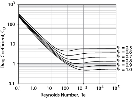
Figure 19.9 Drag Coefficient Dependence on Reynolds Number and Sphericity from Haider and Levenspiel (1989), Equation (19.47)

$where Re = D_{v} u_{t} ρ / μ$ .

The equivalent expression in terms of D* and u_t* is given as

$\begin{matrix} u_{t}^{*} {[\frac{18}{{(D^{*})}^{2}} + \frac{2.335 - 1.745 Ψ}{{(D^{*})}^{0.5}}]}^{- 1} with D^{*} = D_{v} {[\frac{ρ_{f} (| ρ_{s} - ρ_{f} |) g}{μ^{2}}]}^{1 / 3} \end{matrix} (19.48)$

where D_v is the diameter of a sphere with the same volume as the particle.

Equation (19.39) can be solved for one unknown by using either Equation (19.41) or Equation (19.42) for the drag coefficient. For example, the viscosity of a fluid can be determined by measuring the terminal velocity of a falling sphere. Or, the terminal velocity of an object can be determined if all of the fluid and particle physical properties are known. If the Reynolds number is unknown, then the flow regime is unknown. Therefore, depending on the type of problem being solved, judgment may be needed to assume a flow regime, the assumption must be checked, and iterations may be required to get the correct answer.

19.4.2 Fluidized Beds

If fluid flows upward through a packed bed, at a high enough velocity, the particles become buoyant and float in the fluid. For this condition, the upward drag on the particles is equal to the weight of the particles and is called the minimum fluidization velocity, and the particles are said to be fluidized. This is one reason why flow through packed beds is usually downward. The benefits of fluidization are that once the particles are fluidized, they can circulate and the bed of solids mixes. If the upward fluid velocity is sufficiently high, then the bed of particles becomes well mixed (like a continuous stirred tank reactor) and approaches isothermal behavior. For highly exothermic reactions, this property is very desirable. Fluidized beds are often used for such reactions and are discussed in Chapter 22, “Reactors.” Fluidized beds are also used in drying and coating operations where the movement of solids is desirable to increase heat and/or mass transfer. As the fluid velocity upward through the bed of particles increases, the mixing of particles becomes more vigorous and there is a tendency for particles to be flung upward and elutriate from the bed. Therefore, a cyclone is typically part of a fluidized bed to remove the entrained particles and recirculate them to the fluidized bed. Another desirable feature of fluidized beds is that they can be used with very small catalyst particles without a large pressure drop. For very small catalyst particles in a packed bed, the pressure drop becomes very large. An example of such a catalyst is the fluid catalytic cracking catalyst used in petroleum refining to make smaller hydrocarbons from large ones.

The general shape of the pressure drop versus superficial fluid velocity in a fluidized bed is shown in Figure 19.10.

A line graph shows the constant value of the pressure drop above the minimum fluidization velocity.

Figure 19.10 Plot Illustrating Constant Value of Pressure Drop above Minimum Fluidization Velocity

The region to the left of u_mf is described by the Ergun equation for packed beds because, before fluidization begins, behavior is that of a packed bed. If the particles were restricted, by, say, placing a wire screen on top of the bed, then the bed would continue to behave as a packed bed beyond the u_mf. Assuming that the top of the bed is unrestricted, once there is sufficient upward velocity, and hence upward force, the particles begin to lift. This is called minimum fluidization. At minimum fluidization, the upward force is equal to the weight of the particles. Hence, the frictional force equals the weight of the bed, and the pressure drop remains constant. Quantitatively,

$\begin{matrix} - Δ P_{fr} A_{t} = V_{solids} (ρ_{s} - ρ_{f}) g = A_{t} h_{mf} (1 - ε_{mf}) (ρ_{s} - ρ_{f}) g \end{matrix} (19.49)$

where the subscript mf signifies minimum fluidization and h_mf is the height of the bed at minimum fluidization, which for a packed bed is called the length of the bed, L. At the instant at which fluidization begins, the frictional pressure drop is equal to that of a packed bed. Combining Equation (19.19), which is the frictional loss in a packed bed and equals −ΔP_fr/ρ, and Equation (19.49) yields

$\begin{matrix} h_{mt} (1 - ε_{mf}) (ρ_{s} - ρ_{f}) g = \frac{ρ_{f} h_{mf} u_{mf}^{2} (1 - ε_{mf})}{D_{p} ε_{mf}^{3}} [\frac{150 μ (1 - ε_{mf})}{D_{p} μ_{mf} ρ_{f}} + 1.75] \end{matrix} (19.50)$

Rearranging Equation (19.50) and defining two dimensionless groups that characterize the fluid flow in a fluidized bed,

$\begin{matrix} {Re}_{mf} = \frac{D_{p} u_{mf} ρ_{f}}{μ} \end{matrix} (19.51)$

$\begin{matrix} Ar = \frac{D_{P}^{3} ρ (ρ_{s} - ρ_{f}) g}{μ^{2}} \end{matrix} (19.52)$

where Equation (19.51) is the particle Reynolds number, which characterizes the flow regime, and Equation (19.52) defines the Archimedes number, which is the ratio of gravitational forces/viscous forces, yields

$\begin{matrix} \frac{1.75}{ε_{mf}^{3}} {Re}_{mf}^{2} + \frac{150 (1 - ε_{mf})}{ε_{mf}^{3}} {Re}_{mf} - Ar = 0 \end{matrix} (19.53)$

Equation (19.53) is a quadratic in Re_mf, so the minimum fluidization velocity can be obtained if the physical properties of the solid and fluid are known. For nonspherical particles, the result is

$\begin{matrix} \frac{1.75}{Ψ ε_{mf}^{3}} {Re}_{mf}^{2} + \frac{150 (1 - ε_{mf})}{Ψ^{2} ε_{mf}^{3}} {Re}_{mf} - Ar = 0 \end{matrix} (19.54)$

If the void fraction at minimum fluidization, which must be measured, and/or the sphericity are not known, Wen and Yu [12] recommend using

$\begin{matrix} Ψ ε_{mf}^{3} = \frac{1}{14} \end{matrix} (19.55)$

$\begin{matrix} \frac{(1 - ε_{mf})}{Ψ^{2} ε_{mf}^{3}} = 11 \end{matrix} (19.56)$

and Equation (19.54) reduces to

$\begin{matrix} {Re}_{mf} = {[{(33.7)}^{2} + 0.0408Ar]}^{1 / 2} - 33.7 \end{matrix} (19.57)$

Since the volume of solid particles remains constant, it is possible to relate the bed height and void fraction at different levels of fluidization.

$\begin{matrix} h_{mf} (1 - ε_{mf}) = h_{f} (1 - ε_{f}) \end{matrix} (19.58)$

Equation (19.58) is understood by multiplying each side of the equation by A_t, the total bed area, so each side of the equation is the volume of particles because (1 − ε) is the solid fraction, and hA_t is the total bed volume. The operation of fluidized beds above u_mf varies considerably on the basis of the size of particles and the superficial velocity of gas. One way to describe the behavior of these beds is through the flow map by Kunii and Levenspiel [13] in Figure 19.11. In Figure 19.11, u* and D* refer to the dimensionless velocity and particle size introduced in Section 19.4.1, except that the superficial velocity of the gas through the bed (not the particle terminal velocity) is used in u*.

A graph shows the flow regime map for gas-solid fluidization.

The horizontal axis is labeled Dimensionless diameter, D superscript asterisk, ranging from 1 to 100, and the vertical axis is labeled Dimensionless Velocity, u superscript asterisk, ranging from 0.001 to 10, both in increments of the powers of 10. A curve representing Terminal velocity, u subscript t, begins at (1, 0.02) and rises passing through (10, 3) and (100, 10). A curve representing Minimum fluidizing velocity, u subscript (m f) begins at (1.5, 0.002) and rises passing through (50, 1) and (100, 3). Bubbling beds is represented by the plane with the following vertices: (1, 0.05), (1, 0.9), (50, 3), and (50, 1). The terminal velocity curve passes through this plane. Fast fluidized beds is represented by a plane above bubbling bed, with the following vertices: (0.1, 1), (0.1, 7), (10, 10), and (10, 4). Pneumatic transport is a plane overlapping the fast fluidized beds plane. It has the following vertices: (0.5, 2), (0.5, 9), (7, 15), and (7, 4). The coordinate plots are approximate.

Figure 19.11 Flow Regime Map for Gas−Solid Fluidization (Modified from Kunii, D., and O. Levenspiel, Fluidization Engineering, 2nd ed. [Stoneham, MA: ButterworthHeinemann, 1991])

It is clear from this figure that operation of fluidized beds can occur over a wide range of operating velocities from u_mf to several times the terminal velocity. For turbulent (lying above bubbling beds) and fast fluidized beds, internal and external cyclones must be employed, respectively. The gas and solids flow patterns in all these regimes are very complex and can be found only by experimentation or possibly by using complex computational fluid dynamics codes.

19.4.3 Flowrate Measurement

The traditional method for measuring flowrates is to add a restriction in the flow path and measure the pressure drop. The pressure drop can be related to the velocity and flowrate by the mechanical energy balance. More modern instruments include turbine flow meters that measure flowrate directly and vortex shedding devices.

The types of restrictions used are illustrated in Figure 19.12.

Figures show how flowrate is measured using a venturi, a nozzle, and an orifice.

Figure 19.12 Typical Devices Used to Measure Flowrate

The control volume is fluid between an upstream point, labeled 1, and a point in the obstruction, labeled 2. For turbulent flow, the mechanical energy balance written between these two points is

$\begin{matrix} \frac{P_{2} - P_{1}}{ρ} + \frac{u_{2}^{2} - u_{1}^{2}}{2} + e_{f} = 0 \end{matrix} (19.59)$

The friction term is dropped at this point but is incorporated into the problem through a discharge coefficient, C_o. From Equation (19.3), u₁ is expressed in terms of u₂, the cross-sectional areas, and then the diameters; solving for the velocity in the obstruction yields

$\begin{matrix} u_{2} = C_{o} {[\frac{2 (P_{1} - P_{2})}{ρ (1 - β^{4})}]}^{0.5} \end{matrix} (19.60)$

where

$\begin{matrix} β = \frac{D_{2}}{D_{1}} \end{matrix} (19.61)$

The flowrate can then be obtained by multiplying the velocity in the restriction by the cross-sectional area of the restriction. The term C_o, a discharge coefficient, is added to account for the frictional loss in the restriction. Figure 19.13 shows C_o as a function of β and the bore (restriction) Reynolds number for an orifice, one of the most common restrictions used. Since C_o is not known, the asymptotic value of 0.61 for high-bore Reynolds number is assumed, and iterations may be required if the bore Reynolds number is not above about 20,000. This calculation method is illustrated in Example 19.13.

A graph shows the Orifice Discharges Coefficient.

The horizontal axis is labeled Bore Reynolds Number N subscript (R e subscript d) equals (N subscript (R e subscript p)) over beta. It ranges from 1 to 10 to the power of 5, in increments of the powers of 10. The vertical axis is labeled Discharge Coefficient C subscript o, ranging from 0.20 to 1.00, in increments of 0.10. There are nine curves that originate at different between 0.20 and 0.35 along the vertical axis, and on the 4 mark on the horizontal axis. The curves rise to converge at (40, 0.60), from where they continue to rise at different angles in a diverged fashion, such that the top-most curve now becomes the bottom-most. The curves are labeled bottom-up, with their corresponding beta values as follows: 0.2, 0.30, 0.40, 0.5, 0.60, 0.65, 0.70, 0.75, and 0.8. The curves again converge at the point (30000, 0.62), and are again shown to begin to diverge slightly, such that the bottom-most curve now becomes the top-most. All coordinate plots are approximate.

Figure 19.13 Orifice Discharged Coefficient (From Miller, R. W., Flow Measurement Engineering Handbook [New York: McGraw−Hill, 1983] [14])

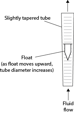
Other flow measurement devices are used. One such device is the rotameter that has a float that moves within a variable area vertical tube. The level of the float in the device is related to the flowrate, as illustrated in Figure 19.14. As the fluid flow increases, the drag on the float increases and it moves up, but the annular flow area around the float also increases. Consequently, the float comes to a new equilibrium position at which its weight is just balanced by the upward drag force of the fluid. Rotameters are still found in laboratories and provide accurate measurements for both gas and liquid flows. While there is a theoretical description of how a rotameter works, it is typically calibrated by measuring the flowrate versus the height of the float for the given fluid of interest.

Figure 19.14 Illustration of Rotameter

Measuring pressure differences is automated in a chemical plant through the use of various devices. However, manometers may still be found in laboratories. Manometers work by having an immiscible fluid of higher density than the flowing fluid in a U-shaped tube, with one end of the tube connected to the pipe at Location 1 and the other end connected as close as possible to Location 2. The height difference between the levels of the immiscible fluid is a measure of the pressure difference between Locations 1 and 2. Figure 19.15 illustrates a general manometer, where the pipe in which the fluid is flowing may be inclined.

Figure 19.15 Illustration of General Manometer Situation

The manometer is an example of fluid statics, so the pressure at any horizontal location must be the same in each manometer leg. For the pressure at height 3 in Figure 19.15,

$\begin{matrix} P_{1} + ρ_{A} g (z_{1} - z_{3}) = P_{2} + ρ_{A} g (z_{2} - z_{4}) + ρ_{B} g (z_{4} - z_{3}) \end{matrix} (19.62)$

Equation (19.62) can be rearranged into the “general” manometer equation:

$\begin{matrix} P_{1} - P_{2} + g Δ h (ρ_{A} - ρ_{B}) + ρ_{A} g (z_{1} - z_{2}) = 0 \end{matrix} (19.63)$

where

$\begin{matrix} Δ h = (z_{4} - z_{3}) \end{matrix} (19.64)$

The third term in Equation (19.63) is zero if the pipe is horizontal. It is important to understand that z₁ − z₂ is a difference in vertical distance (height), not a distance along the pipe, and that the coordinate system points upward, so a high height minus a low height is a positive number.

Example 19.13

An orifice having a diameter of 1 in is used to measure the flowrate of an oil (SG = 0.9, μ = 50 cP) in a horizontal, 2-in, schedule-40 pipe at 70°F. The pressure drop across the orifice is measured by a mercury (SG = 13.6) manometer, which reads 2.0 cm. Calculate the volumetric flowrate of the oil.

Solution

Two steps are involved. First, the pressure drop is calculated from the manometer information. Then, the flowrate is calculated.

To calculate the pressure drop, Equation (19.62) is used, but since the pipe is horizontal, the third term on the right-hand side is zero. The result is

$\begin{matrix} \begin{matrix} P_{1} - P_{2} = g Δ h (ρ_{B} - ρ_{A}) = \\ \frac{{32.2 ft/sec}^{2}}{{32.2 ft lb/lb}_{f} {/sec}^{2}} (2 cm \frac{1 in}{2.54 cm}) (13.6 - {0.9)(62.4 lb/ft}^{3}) {(\frac{ft}{12 in})}^{3} = 0.361 psi \end{matrix} & (E19.13a) \end{matrix}$

Next, the pressure drop is used in Equation (19.60) with the initial assumption that C_o = 0.61. So

$\begin{matrix} u_{2} = 0.61 [\frac{{2(0.361 lb}_{f} {/in}^{2} {)(12 in/ft)}^{2} {(32.2 ft lb/lb}_{f} {/sec}^{2})}{{0.9(62.4 lb/ft}^{3}) [1 - {(\frac{1 in}{2.067 in})}^{4}]}] = 4.84 ft/sec & (E19.13b) \end{matrix}$

Now, the bore Reynolds number must be checked.

$\begin{matrix} Re = \frac{{(1/12 ft)(4.84 ft/sec)(62.4 lb/ft}^{3})}{50 cP (6.72 \times 10^{- 4} lb/ft/sec/cP)} = 749 & (E19.13c) \end{matrix}$

From Figure 19.13, with β = 0.48 and Re = 749, C_o ≈ 0.71. Repeating the calculation in Equation (E19.11b) gives u₂ = 5.63 ft/sec and Re = 872. Within the error of reading Figure 19.12, C_o ≈ 0.71, so the iteration is completed. The volumetric and mass flowrates can now be calculated:

$\begin{matrix} \dot{v} = {(5.63 ft/sec)(0.02330 ft}^{2} {) = 0.131 ft}^{3} /sec & (E19.13d) \end{matrix}$

$\begin{matrix} \dot{m} = {(0.131 ft}^{3} {/sec)(62.4 lb/ft}^{3}) = 8.19 lb/sec & (E19.13e) \end{matrix}$

When fluid flows through an orifice, the pressure decreases because the velocity increases through the small cross-sectional area of the orifice. Physically, this is because pressure energy is converted to kinetic energy. This is similar to a nozzle, as illustrated in Example 19.3. Subsequently, when the velocity decreases as the cross-sectional area increases to the total pipe area, the pressure increases again. However, not all of the pressure is “recovered,” due to circulating fluid flow at the pipe-orifice diameter. The permanent pressure loss requires incremental pump power, and that is part of the cost of measuring the flowrate using an orifice or nozzle. The amount of recovered pressure has been correlated as a function of β for different flow measuring devices, and it is illustrated in Figure 19.16.

A graph shows the unrecovered frictional loss in different glow measuring devices.

The horizontal axis is labeled Beta Ratio, beta, ranging from 0 to 0.8, in increments of 0.1. The vertical axis is labeled Permanent Pressure Loss-Percent of Differential, ranging from 1 to 10 in unit increments, and from 10 to 100, in increments of 10. The curve pertaining to Square edge orifice begins at (0, 100) and curves gradually down to (0.76, 45). The Flow nozzle curve begins at (0.32, 82) and curves down almost along the previous curve to (0.76, 36). These two curves are concave, while the next two are convex. The curves pertaining to Venturi 15 degree exit cone and Herschel Venturi 7 degree exit cone, begin at (0.2, 30) and (0.2, 15) respectively, and curve down accordingly to meet at (0.76, 13). The V over (V T) curve begins at (0.34, 7.8) and curves in a concave fashion to (0.76, 3.9). The curve pertaining to L o loss begins at (0.3, 8) and curves in a convex fashion to (0.76, 2.6). All coordinate plots are approximate.

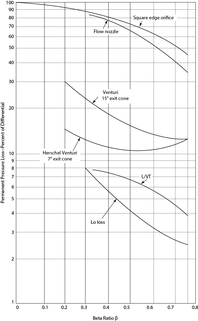
Figure 19.16 Unrecovered Frictional Loss in Different Flow Measuring Devices (Adapted by permission from Cheremisinoff, N. P., and P. N. Cheremisinoff, Instrumentation for Process Flow Engineering [Lancaster: Technomic, 1987] [15])

Example 19.14

For Example 19.13, how much additional power is needed for the permanent pressure loss through the orifice? The pump is 75% efficient.

Solution

For β ≈ 0.5, from Figure 19.16, the permanent pressure loss is about 73%. From the mechanical energy balance,

$\begin{matrix} \frac{0.73 (P_{1} - P_{2})}{ρ} - \frac{η_{p} {\dot{W}}_{s}}{\dot{m}} = 0 & (E19.14a) \end{matrix}$

$\begin{matrix} \frac{{(0.73)(0.361 lb}_{f} {/in}^{2} {)(12 in/ft)}^{2}}{{0.9(62.4 lb/ft}^{3})} = \frac{0.75 {\dot{W}}_{s}}{8.19 lb/sec} & (E19.14b) \end{matrix}$

$\begin{matrix} {\dot{W}}_{s} = {7.38 ft lb}_{f} /sec = 0.0134 hp & (E19.14c) \end{matrix}$

This result shows that, while there is a cost associated with an orifice, it is small.

19.5 Performance of Fluid Flow Equipment

In addition to equipment design, the chemical engineer must deal with the performance of existing equipment. The differences between the design problem (also called a rating problem) (a) and the performance problem (b) are illustrated in Figure 19.17. The use of italics indicates the unknowns in the particular problem. In the design problem, the input and the desired output are specified, and the equipment is designed to satisfy those constraints. In the performance problem, the input and equipment are specified, and the output is determined. The performance problem is what is involved in dealing with day-to-day operations in a chemical plant.

Figures a and b show the same system, that has an Input given to Equipment specifications, and an Output leaving it. In figure a, "Equipment specifications" is shown in italics, while in figure b the Output is shown in italics.

Figure 19.17 Illustrations of (a) Design Problem and (b) Performance Problem (Unknowns Are Indicated by Italics for Each Case)

Several different types of problems in frictional fluid flow using the mechanical energy balance were discussed in Section 19.3. Determining the pump power needed for a given situation is a design problem. Similarly, determining the required pipe diameter is a design problem. On the other hand, determining the flowrate when all equipment is specified is a performance problem, as is determining the pressure change for an existing system.

Suppose it is necessary to increase the capacity of a process without adding new equipment. Logically, all flowrates must increase. This is a performance problem, since the input and equipment are specified, and the output must be determined for each unit in the process. Somewhere in the process, the amount of scale-up needed will be limited due to equipment constraints, and this limiting unit is called a bottleneck. The process of finding a solution that removes the bottleneck is called debottlenecking, which is a performance problem. Similarly, if there is a problem with the output of a process (purity or temperature, for example), the cause of the problem must be determined, which is called troubleshooting.

Returning to the situation in which process capacity must be increased, for the fluid flow component, initially, it may appear that problems similar to those in Section 19.3 must be solved from scratch. However, for many situations, not just in fluid flow, very good approximations can be made with a much simpler analysis.

19.5.1 Base-Case Ratios

The ability to predict changes in a process design or in plant operations is improved by anchoring an analysis to a base case. This calculation tool combines use of fundamental relationships with plant operating data to form a basis for predicting changes in system behavior. As will be seen, it is applicable to problems involving all chemical process units when analytical expressions are available.

For design changes, it is desirable to identify a design proven in practice as the base case. For operating plants, actual data are available and are chosen as the base case. It is important to put this base case into perspective. Assuming that there are no instrument malfunctions and these operating data are correct, then these data represent a real operating point at the time the data were taken. As the plant ages, the effectiveness of process units changes and operations are altered to account for these changes. As a consequence, recent data on plant operations should be used in setting up the base case.

The base-case ratio integrates the “best available” information from the operating plant with design relationships to predict the effect of process changes. It is an important and powerful technique with a wide range of applications. The base-case ratio, X, is defined as the ratio of a new-case system characteristic, x₂, to the base-case system characteristic, x₁:

$\begin{matrix} X \equiv x_{2} / x_{1} \end{matrix} (19.65)$

Using a base-case ratio often reduces the need for knowing actual values of physical properties (physical properties refer to thermodynamic and transport properties of fluids), equipment, and equipment characteristics. The values identified in the ratios fall into three major groups. They are defined below and applied in Examples 19.15 and 19.16.

Ratios Related to Equipment Sizes (equivalent length, L_eq; diameter, D; surface area, A): Assuming that the equipment is not modified, these values are constant, the ratios are unity, and these terms cancel out.
Ratios Related to Physical Properties (such as density, ρ; viscosity, μ): These values can be functions of material composition, temperature, and pressure. Only the functional relationships, not absolute values, are needed. For small changes in composition, temperature, or pressure, the properties often are unchanged, and the ratio is unity and cancels out. An exception to this is gas-phase density.
Ratios Related to Stream Properties: These ratios usually involve velocity, flowrate, concentration, temperature, and pressure.

Using the base-case ratio eliminates the need to know equipment characteristics and reduces the amount of physical property data needed to predict changes in operating systems.

The base-case ratio is a powerful and straightforward tool to analyze and predict process changes. This is illustrated in Example 19.15.

Example 19.15

It is necessary to scale up production in an existing chemical plant by 25%. Your job is to determine whether a particular pump has sufficient capacity to handle the scale-up. The pump’s function is to provide enough pressure to overcome frictional losses between the pump and a reactor.

Solution

The relationship for frictional pressure drop is obtained from the mechanical energy balance:

$\begin{matrix} \frac{Δ P}{ρ} = - \frac{2 fL u^{2}}{D} & (E19.15a) \end{matrix}$

This relationship is now written as the ratio of two cases, where subscript 1 indicates the base case, and subscript 2 indicates the new case:

$\begin{matrix} \frac{Δ P_{2}}{Δ P_{1}} = \frac{2 ρ_{2} f_{2} L_{eq 2} u_{2}^{2} D_{1}}{2 ρ_{1} f_{1} L_{eq 1} u_{1}^{2} D_{1}} & (E19.15b) \end{matrix}$

Because the pipe has not been changed, the ratios of diameters (D₂/D₁) and lengths (L_eq₂/L_eq₁) are unity. Because a pump is used only for liquids, and liquids are (practically) incompressible, the ratio of densities is unity. If the flow is assumed to be fully turbulent, which is usually true for process applications, the friction factor is not a function of Reynolds number. This fact should be checked for a particular application. Figure 19.6 illustrates how, for fully turbulent flow in pipes that are not hydraulically smooth, the friction factor approaches a constant value. Since the x-axis is a log scale, changes up to a factor of 2 to 5, which are well beyond the scale-up capability of most equipment, do not represent much of a difference on the graph. Therefore, the friction factor is constant, and the ratio of friction factors is unity. The ratio in Equation (E19.15b) reduces to

$\begin{matrix} \frac{Δ P_{2}}{Δ P_{1}} = \frac{u_{2}^{2}}{u_{1}^{2}} = \frac{{\dot{m}}_{2}^{2} / A_{2}^{2} ρ_{2}^{2}}{{\dot{m}}_{1}^{2} / A_{1}^{2} ρ_{1}^{2}} = \frac{{\dot{m}}_{2}^{2}}{{\dot{m}}_{1}^{2}} & (E19.15c) \end{matrix}$

where the second equality is obtained by substituting for u_i in numerator and denominator using the mass balance ${\dot{m}}_{i} = ρ_{i} A_{i} u_{i}$ , canceling the ratio of densities for the same reason as above, and canceling the ratio of cross-sectional areas because the pipe has remained unchanged. Therefore, by assigning the base-case mass flow to have a value of 1, for a 25% scale-up, the new case has a mass flow of 1.25, and the ratio of pressure drops becomes

$\begin{matrix} \frac{Δ P_{2}}{Δ P_{1}} = {(\frac{{\dot{m}}_{2}}{{\dot{m}}_{1}})}^{2} = {(\frac{1.25}{1})}^{2} = 1.56 & (E19.15d) \end{matrix}$

Thus, the pump must be able to deliver enough head to overcome 56% additional frictional pressure drop while pumping 25% more material.

It is important to observe that Example 19.15 was solved without knowing any details of the system. The pipe diameter, length, and number of valves and fittings were not known. The liquid being pumped, its temperature, and its density were not known. Yet the use of base-case ratios along with simple assumptions permitted a solution to be obtained. This illustrates the power and simplicity of base-case ratios.

Example 19.16

It is proposed to improve performance through a section of pipe by adding an identical section in parallel.

If the total flowrate remains constant, what parameter changes and by how much, assuming the fluid flow is fully turbulent?
If the original pipe is 1.5-in, schedule-40, commercial steel, and the new section is 2-in, schedule-40, commercial steel, answer the same question as in Part (a).

Solution

By using the mechanical energy balance and Equation (19.14) for the friction term, with the subscript 1 representing the original case and subscript 2 representing the new case, each being the flow through the original section, the ratio of pressure drops is

$\begin{matrix} \frac{Δ P_{2}}{Δ P_{1}} = \frac{- e_{f 2}}{- e_{f 1}} = \frac{32 ρ_{2} f_{2} L_{eq 2} {\dot{v}}_{2}^{2}}{π^{2} D_{2}^{5}} \frac{π^{2} D_{1}^{5}}{32 ρ_{1} f_{1} L_{eq 1} {\dot{v}}_{1}^{2}} & (E19.16a) \end{matrix}$

The constants cancel. If the fluid is unchanged, the densities cancel. Since the new and old pipe lengths and diameters are identical, the lengths and diameters cancel. It is assumed that the minor losses due to the elbows and fitting needed to add the parallel pipe are unchanged, so the equivalent lengths cancel. For fully turbulent flow, the friction factor has asymptotically approached a constant value (Figure 19.6), so the friction factors cancel. So, the result is

$\begin{matrix} \frac{Δ P_{2}}{Δ P_{1}} = \frac{{\dot{v}}_{2}^{2}}{{\dot{v}}_{1}^{2}} & (E19.16b) \end{matrix}$

Since the two parallel sections are identical, the flowrate splits equally between the two sections, so the flowrate in the original section is half of the original flowrate:

$\begin{matrix} \frac{Δ P_{2}}{Δ P_{1}} = \frac{{\dot{v}}_{2}^{2}}{{\dot{v}}_{1}^{2}} = \frac{{(0.5 {\dot{v}}_{1})}^{2}}{{\dot{v}}_{1}^{2}} = 0.25 & (E19.16c) \end{matrix}$

Therefore, the pressure drop through that section of pipe decreases by 75%.
In this case, subscripts 1 and 2 represent the flow though the original and new sections, after the parallel section is installed. The analysis starts identically, but the diameters and friction factors do not cancel. The friction factors do not cancel because the asymptotic value for the friction factor in Figure 19.6 and in the Pavlov equation (Equation [19.16]) depends on the ratio of the roughness factor to the diameter, and that ratio is different for the two sections of pipe. The ratio expression becomes

$\begin{matrix} \frac{Δ P_{2}}{Δ P_{1}} = \frac{f_{2} {\dot{v}}_{2}^{2} D_{1}^{5}}{f_{2} {\dot{v}}_{1}^{2} D_{2}^{5}} & (E19.16d) \end{matrix}$

From the Pavlov equation (Equation [19.16]), using the ratio of the friction factors at an asymptotically large Reynolds number and the schedule pipe diameters, Equation (E19.16d) becomes

$\begin{matrix} \frac{Δ P_{2}}{Δ P_{1}} = {[\frac{\log_{10} (\frac{0.0018 in}{3.7(1.610 in)})}{\log_{10} (\frac{0.0018 in}{3.7(2.067 in)})}]}^{2} \frac{{(1.610 in)}^{5} {\dot{v}}_{2}^{2}}{{(2.067 in)}^{5} {\dot{v}}_{1}^{2}} = 0.270 \frac{{\dot{v}}_{2}^{2}}{{\dot{v}}_{1}^{2}} & (E19.16e) \end{matrix}$

Since the pressure drops in each parallel section must be equal,

$\begin{matrix} \frac{{\dot{v}}_{2}}{{\dot{v}}_{1}} = {(\frac{1}{0.270})}^{0.5} = 1.92 \end{matrix} (E19.16f)$

If the flow is laminar, the analysis would be similar, but the results would differ due to the different expression for the friction factor in laminar flow. Examples of this are the subject of problems at the end of the chapter.

19.5.2 Net Positive Suction Head

There is a significant limitation on pump operation called net positive suction head (NPSH). This is the head that is needed on the pump feed (suction) side to ensure that liquid does not vaporize upon entering the pump. Its origin is as follows. Although the effect of a pump is to raise the pressure of a liquid, frictional losses at the entrance to the pump, between the suction pipe and the internal pump mechanism, cause the liquid pressure to drop upon entering the pump. This means that a minimum pressure exists somewhere within the pump. If the feed liquid is saturated or nearly saturated, the liquid can vaporize upon entering due to this internal pressure drop. This causes formation of vapor bubbles. These bubbles rapidly collapse when exposed to the forces created by the pump mechanism, called cavitation. This process usually results in noisy pump operation and, if it occurs for a period of time, will damage the pump. As a consequence, regulating valves, which lower fluid pressure, are not normally placed in the suction line to a pump.

Pump manufacturers supply NPSH data with a pump, usually in head units. In this book, both head and pressure units are used. The required NPSH, denoted NPSH_R, is a function of the square of velocity because it is a frictional loss and because most applications involve turbulent flow. Figure 19.18(a) shows NPSH_R and NPSH_A curves, which define a region of acceptable pump operation. This is specific to a given liquid. Typical NPSH_R values are in the range of 15 to 30 kPa (2-4 psi) for small pumps and can reach 150 kPa (22 psi) for larger pumps. Figure 19.18 also shows curves for NPSH_A, the available NPSH, along with the NPSH_R curve.

Two graphs show the region of feasible operation of the N P S H subscript A and the N P S H subscript R curves, and the physical parameters that affect the shape of the prior.

Both graphs have the horizontal axis labeled Velocity, u (meters per second), ranging from 0 to 8, in increments of 2, and the vertical axis labeled N P S H (bar), ranging from 0.0 to 1.2, in increments of 0.2. In figure a, the N P S H subscript A curve begins at (0, 1.1) and curves in a concave manner to (7.5, 0.0), and the N P S H subscript R curve begins at (0, 0.0) and curves in a convex manner to (8, 0.8). The two curves meet at (5.9, 0.4) and a perpendicular line is drawn through this point. The areas before and after the perpendicular are labeled as follows, respectively: Region of acceptable operation and Region of unacceptable operation due to cavitation. In figure b, the two curves are shown as in figure a, and the N P S H subscript A curve is said to have the following parameters: 1-inch schedule 40, h equals 3 meters, 57 degrees Celsius. The curve is labeled b. Two more N P S H subscript A curves are shown from (0, 1.1) to (7, 0.0) and (8, 0.1), labeled a and c respectively. Curve a has the following parameters: 1-inch schedule 40, h equals 2 meters, 57 degrees Celsius. The points where curves a, b, and c, meet the N P S H subscript R curve are marked in the respective uppercase letters. All coordinate plots are approximate.

Figure 19.18 (a) NPSH_A and NPSH_R Curves Showing Region of Feasible Operation; (b) How Physical Parameters Affect Shape of NPSH_A Curve

The available NPSH_A is defined as

$\begin{matrix} NPS H_{^{A}} = P_{inlet} - P^{*} \end{matrix} (19.66)$

Equation (19.66) means that the available NPSH (NPSH_A) is the difference between the inlet pressure, P_inlet, and P*, which is the vapor pressure (bubble-point pressure for a mixture). It is required that NPSH_A ≥ NPSH_R to avoid cavitation. Cavitation is avoided if operation is to the left of the intersection of the two curves. It is physically possible to operate to the right of the intersection of the two curves, but doing so is not recommended because the pump will be damaged.

All that remains is to calculate or know the pump inlet conditions in order to determine whether sufficient NPSH (NPSH_A) is available to equal or exceed the required NPSH (NPSH_R). For example, consider the exit stream from a distillation column reboiler, which is saturated liquid. If it is necessary to pump this liquid, cavitation could be a problem. A common solution to this problem is to elevate the column above the pump so that the static pressure increase minus any frictional losses between the column and the pump provides the necessary NPSH to avoid cavitation. This can be done either by elevating the column above ground level using a metal skirt or by placing the pump in a pit below ground level, although pump pits are usually avoided due to safety concerns arising from accumulation of heavier-than-air gases in the pit.

In order to quantify NPSH, consider Figure 19.19, in which material in a storage tank is pumped downstream in a chemical process. This scenario is a very common application of the NPSH concept. For NPSH analysis, the only portion of Figure 19.19 under consideration is between the tank and pump inlet.

An illustration of the application of the N P S H principles.

Figure 19.19 Typical Situation for Application of NPSH Principles

From the mechanical energy balance, the pressure at the pump inlet can be calculated to be

$\begin{matrix} P_{inlet} = P_{tank} + ρ gh - \frac{2 ρ f L_{eq} u^{2}}{D} \end{matrix} (19.67)$

which means that the pump inlet pressure is the tank pressure plus the static pressure minus the frictional losses in the suction-side piping. Therefore, by substituting Equation (19.67) into Equation (19.66), the resulting expression for NPSH_A is

$\begin{matrix} NPS H_{A} = P_{tank} + ρ gh - \frac{2 ρ f L_{eq} u^{2}}{D} - P * \end{matrix} (19.68)$

This is an equation of a concave downward parabola, of the form $NPS H_{A} = a - b u^{2}$ , as illustrated in Figure 19.18(b), Curve a. The intercept is a = P_tank + pgh − P* and b = 2ρfL_eq/D. This analysis does not include the kinetic energy term due to the acceleration of the fluid from the tank into the pipe. Rigorously, this term should also be included in the analysis.

If NPSH_A is insufficient for a particular situation, Equation (19.68) suggests methods to increase the NPSH_A:

Decrease the temperature of the liquid at the pump inlet. This decreases the value of the vapor pressure, P*, thereby increasing NPSH_A. This increases the intercept of the NPSH_A curve while maintaining constant curvature, as illustrated in Figure 19.18(b), Curve b.
Increase the static head. This is accomplished by increasing the value of h in Equation (19.64), thereby increasing NPSH_A. As was said earlier, pumps are most often found at lower elevations than the source of the material they are pumping. This increases the intercept of the NPSH_A curve while maintaining constant curvature, as illustrated in Figure 19.18(b), Curve b.
Increase the tank pressure. This increases the intercept of the NPSH_A curve while maintaining constant curvature, as illustrated in Figure 19.18(b), Curve b.
Increase the diameter of the suction line (feed pipe to pump). This reduces the velocity and the frictional loss term, thereby increasing NPSH_A. This decreases the curvature of the NPSH_A curve, as illustrated in Figure 19.18(b), Curve c. It is standard practice to have larger-diameter pipes on the suction side of a pump than on the discharge side.

Example 19.17 illustrates how to do NPSH calculations and one of the preceding methods for increasing NPSH_A. The other methods are illustrated in problems at the end of the chapter.

Example 19.17

A pump is used to transport toluene at 10,000 kg/h from a feed tank (V-101) maintained at atmospheric pressure and 57°C. The pump is located 2 m below the liquid level in the tank, and there is 6 m of equivalent pipe length between the tank and the pump. It has been suggested that 1-in, schedule-40, commercial-steel pipe be used for the suction line. Determine whether this is a suitable choice. If not, suggest methods to avoid pump cavitation.

Solution

The following data can be found for toluene: ln P*(bar) = 10.97 − 4203.06/T(K), μ = 4.1 × 10^-4 kg/m s, ρ = 870 kg/m³. For 1-in, schedule-40, commercial-steel pipe, the roughness factor is about 0.001 and the inside diameter is 0.02664 m. Therefore, the velocity of toluene in the pipe can be found to be 5.73 m/s. The Reynolds number is about 426,000, and the friction factor is f = 0.005. At 57°C, the vapor pressure is found to be 0.172 bar.

From Equation (19.68),

$\begin{matrix} NPS H_{A} = 1.01325 bar + {870(9.81)(2)(10}^{- 5}) bar \\ - 2 (870) (0.005) (6) {(5.73)}^{2} (10^{- 5}) / (0.02664) bar - 0.172 bar \\ NPS H_{A} = 0.37 bar \end{matrix}$

This is shown as Point A on Figure 19.18(b). At the calculated velocity, Figure 19.18(b) shows that NPSH_R is 0.40 bar, Point B. Therefore, there is insufficient NPSH_A. This means that a 1-in, schedule-40 pipe is unacceptable for this service.

The obvious solution to this problem is to use a larger-diameter pipe for the suction side of the pump. The calculated velocity of 5.73 m/s is far in excess of the typical maximum liquid velocity. The frictional loss in the 6 m of suction piping is approximately 0.64 bar. If, say, a 2-in, schedule-40 pipe was used for the suction line, then the frictional loss would decrease to approximately 0.02 bar and NPSH_A would increase to about 0.99 bar, which is far in excess of NPSH_R. Another method for increasing NPSH_A is to increase the height of liquid in the tank. If the height of liquid in the tank is 3 m, with the original 1-in, schedule-40 pipe at the original temperature, NPSH_A = 0.445 bar. This is shown as Point C on Figure 19.18(b).

19.5.3 Pump and System Curves

Pumps also have characteristic performance curves, called pump curves. Figure 19.20 illustrates a pump curve for a centrifugal pump. Centrifugal pumps are often called constant head pumps because, over a wide range of volumetric flowrates, the head produced by the pump is approximately constant. Pump manufacturers provide the characteristic curve, usually in head units. For centrifugal pumps, the shape of the curve indicates that although the head remains constant over quite a wide range of flowrates, eventually, as the flowrate continues to increase, the head produced decreases. Pump curves also include power and efficiency curves, both of which change with flowrate and head; however, these are not shown here.

A line graph shows the shape of a pump curve for a centrifugal pump. The horizontal and vertical axes are labeled Flowrate and Head, respectively. The curve begins from the upper part of the vertical axis, continues as a straight line and curves down smoothly at about two-thirds the length of the horizontal axis.

Figure 19.20 Typical Shape of Pump Curve for Centrifugal Pump

For a piping system, a system curve can also be defined. Consider the system as illustrated in Figure 19.21. Location 1 is called the source, and Location 2 is the destination. Location 2 may be distant from Location 1, perhaps at the opposite end of a chemical process and at a different elevation from Location 1. Typical processes have only one pump upstream to supply all pressure needed to overcome pressure losses throughout the process. Therefore, the pressure increase across the pump must be sufficient to overcome all of the losses associated with piping and fittings plus the indicated pressure loss across the control valve. The orifice plate is present to illustrate some type of flowrate measurement, and the flow indicator controller (FIC) illustrates that the measured flowrate is compared to a set point, and deviations from the set point are compensated by adjusting the valve, usually pneumatically. If the flowrate is too large, the valve is partially closed, restricting the flowrate. However, this also increases the frictional pressure loss across the valve, as discussed in Section 19.3.2.

An illustration of the physical setup for a system curve.

Figure 19.21 Physical Situation for System Curve

The behavior of the system can be quantified by a system curve. The general equation for a chemical process, in terms of pressure, is given by the mechanical energy balance between Points 1 and 2 in Figure 19.21:

$\begin{matrix} Δ P_{pump} = Δ P_{12} + ρ g Δ z_{12} + (- Δ P_{f}) + (- Δ P_{cv}) = (P_{2} - P_{1}) + ρ g (z_{2} - z_{1}) + (- Δ P_{f}) + (- Δ P_{cv}) \end{matrix} (19.69)$

where

$\begin{matrix} - Δ P_{fr} = ρ e_{f} = \frac{2 ρ f L_{eq} u^{2}}{D} \end{matrix} (19.70)$

Equation (19.70) is derived from the mechanical energy balance with only the pressure and friction terms. It is important to remember that Δ represents out-in; therefore, the frictional loss term and the pressure loss across the valve are negative numbers before the included negative sign. The system curve is the right-hand side of Equation (19.69) without the term for the control valve:

$\begin{matrix} Δ P_{system} = (P_{2} - P_{1}) + ρ g (z_{2} - z_{1}) + (- Δ P_{fr}) = (P_{2} - P_{1}) + ρ g (z_{2} - z_{1}) + \frac{32 ρ f L_{eq} {\dot{v}}^{2}}{π^{2} D^{5}} \end{matrix} (19.71)$

Equation (19.71) is a parabola, concave upward, on a plot of pressure increase versus flowrate. It is of the form $Δ P_{system} = a + b {\dot{v}}^{2}$ , where a = (P₂ − P₁) + ρ g(z₂ −z₁) and $b = 32 ρ f L_{eq} / (π^{2} D^{5})$ . Since the manufacturer pump curve is usually provided in head units, Equation (19.69) can be rewritten in head units as

$\begin{matrix} h_{system} = \frac{Δ P_{system}}{ρ g} = \frac{(P_{2} - P_{1})}{ρ g} + (z_{2} - z_{1}) + \frac{32 f L_{eq} {\dot{v}}^{2}}{g π^{2} D^{5}} \end{matrix} (19.72)$

Figure 19.22 illustrates the result if the pump curve and the system curve are plotted on the same graph. The indicated pressure changes demonstrate how the head provided by the pump must equal the desired head increase from source to destination, plus the frictional pressure loss, plus the pressure loss across the control valve, as quantified in Equation (19.69). The process of flowrate regulation is also illustrated in Figure 19.22. If the flowrate is to be reduced, the valve is closed, and the operating point moves to the left. At this lower flowrate, the frictional losses are lower, but the pressure loss across the valve is larger. The opposite is true for a higher flowrate. At the intersection of the two curves, the valve is wide open, and the maximum possible flowrate has been reached. This analysis assumes that the pump is operating at constant speed. For a variable speed pump, the pump curve moves up or down as the speed of rotation of the impeller changes. (Note that this simplified explanation omits the very small pressure drop across a wide-open control valve.) Operation to the right of this point is impossible. It is important not to confuse the meanings of the intersection points on the pump-system curve plot and the NPSH plot.

A graph showing the components of the pump and system curves.

The horizontal and vertical axes are labeled Volumetric flowrate and Head, respectively. The pump curve for a centrifugal pump begins from the upper part of the vertical axis, continues as a straight line and curves down smoothly at about two-thirds the length of the horizontal axis. The system curve is a mirror image of the pump curve, drawn below it. The point where the two curves intersect is labeled Maximum possible flowrate. A perpendicular to the horizontal axis is drawn through this point and is labeled Impossible operation delta P subscript pump lesser than delta P subscript sys. A line parallel to the horizontal axis is drawn from the starting point of the system curve. This point is labeled delta P subscript (source-dest) plus rho g times delta z. Another perpendicular is drawn to the horizontal axis at the Operating point, cutting both the curves at the points the begin to turn. The point where the perpendicular cuts the pump curve is delta P subscript pump. Negative delta P subscript friction is the distance between the parallel line and the system curve, just past the perpendicular from the Operating point. The distance between the two curves, just within this perpendicular is negative P subscript valve.

Figure 19.22 Pump (Constant Speed Centrifugal Pump) and System Curve Components

The pump and system curve plot also illustrates the cost of flowrate regulation. The pump must provide sufficient pressure to overcome the losses across the valve over a wide range of flowrates. Additional pump power is required for the possibility of operating at lower flowrates with a very large pressure drop across the valve. In general, this is a small cost for a pump, because the liquid density is high. Variable speed pumps are also available with different pump curves for different speeds. For these, the flowrate is regulated by the rotation speed of the impeller, not by a valve. It is not usually worth the extra cost for small pumps given the low cost of pumping liquids but may be worth considering for larger pumps and flowrates. Pumps with different impeller sizes have different pump curves for each impeller size. However, changing an impeller is not something that can be done while a process is operating.

Pumps (and compressors) are about the only pieces of equipment in a chemical plant with moving parts. Moving parts can fail. Therefore, since pumps are often inexpensive (on the order of $10,000), a backup pump is typically installed in parallel so the plant can continue operating while the primary pump is maintained. Since shutdown and start-up can take days, it makes sense not to shut down a process that generates profit at a rate of thousands of dollars per minute to avoid purchasing a relatively inexpensive backup pump.

The presence of a backup pump can also be exploited if is necessary to scale-up a process. The piping system can be constructed such that the two pumps can operate simultaneously, either in series or in parallel. If the pumps are in series, the head increase doubles at the same flowrate. If the pumps are in parallel, the flowrate doubles at the same head increase. The pump curves for these situations are illustrated in Figure 19.23. The two system curves illustrate the maximum possible scale-up for two different system curves, indicated by the dots. In one case, the parallel configuration provides more scale-up potential, and in the other case, the series configuration provides more scale-up potential. This demonstrates that it is not possible to make any generalizations about which configuration can produce more scale-up. It all depends on the particular system.

A graph shows the pump and system curves for series and parallel pumps.

The horizontal and vertical axes are labeled Volumetric flowrate and Head, respectively. Two system curves are shown originating at a point from the lower parts of the vertical axis and rise gradually at different angles. The Pump curve for two pumps in series begins at a point toward the very top of the vertical axis, and curves smoothly down to touch the horizontal axis at almost its mid-point. The point where this curve cuts the first system curve is marked. The Pump curve for two pumps in parallel originates at about the mid-point of the vertical axis, declines slightly and falls steeply toward the end of the horizontal axis. The point where this curve cuts the second system curve is marked. The Pump curve for a single pump originates at the same point as the pump curve for two parallel pumps and gradually falls to end at the same point as the pump curve for two serial pumps.

Figure 19.23 Pump and System Curves for Series and Parallel Pumps

Positive-displacement pumps perform differently from centrifugal pumps. They are usually used to produce higher pressure increases than are obtained with centrifugal pumps. The performance characteristics are represented on Figure 19.24(a), and these are sometimes referred to as constant-volume pumps. It can be observed that the flowrate through the pump is almost constant over a wide range of pressure increases, which makes flowrate control using the pressure increase impractical. One method to regulate the flow through a positive-displacement pump is illustrated in Figure 19.24(b). The strategy is to maintain constant flowrate through the pump. By regulating the flow of the recycle stream to maintain constant flowrate through the pump, the downstream flowrate can be regulated independently of the flow through the pump. Therefore, if a higher flow to the process is needed, then the bypass control valve is closed, and vice versa.

A graph shows the pump curve for the positive-displacement pump and a figure shows the setup for flowrate regulation.

Figure 19.24 (a) Typical Pump Curve for Positive−Displacement Pump and (b) Method for Flowrate Regulation

It is observed from Figure 19.21 and Figure 19.24 that, in both cases, flowrate regulation occurs by adjusting a valve. For regulation of temperature, a valve on a cooling or heating fluid is adjusted. For regulation of concentration, valves on mixing streams are adjusted. This emphasizes the concept that about the only way to regulate anything in a chemical process is to adjust a valve position.

Process conditions are usually regulated or modified by adjusting valve settings in the plant..

Example 19.18

Develop the system curve for flow of water at approximately 10 kg/s through 100 m of 2-in, schedule-40, commercial-steel pipe with the source and destination at the same height and both at atmospheric pressure.

Solution

The density of water will be taken as 1000 kg/m³, and the viscosity of water will be taken as 1 mPa s (0.001 kg/m s). The inside diameter of the pipe is 0.0525 m. The Reynolds number can be determined to be 2.42 × 10⁵. For a roughness factor of 0.001, f = 0.005. Equation (19.71) reduces to

$\begin{matrix} Δ P = - 19 u^{2} & (E19.18a) \end{matrix}$

since ΔP_1-3 is zero, with ΔP in kPa and u in m/s. This is the equation of a parabola, and it is plotted in Figure E19.18. Therefore, from either the equation or the graph, the frictional pressure drop is known for any velocity.

A graph shows the system curves for some examples.

Figure E19.18 System Curves for Examples 19.18 and 19.19

Example 19.19

Repeat Example 19.18 for the same length of pipe but with a 10 m vertical elevation change, with the flow from lower to higher elevation, but with the source and destination both still at atmospheric pressure.

Solution

Here, the potential energy term from the mechanical energy balance must be included. The magnitude of this term is 10 m of water, so ρgΔz = 98 kPa. Equation (19.69) reduces to

$\begin{matrix} Δ P = - (98 + 19 u^{2}) \end{matrix} (E19.19)$

with ΔP in kPa and u in m/s. This equation is also plotted in Figure E19.18. It is observed that the system curve has the same shape as that in Example 19.18. This means that the frictional component is unchanged. The difference is that the entire curve is shifted up by the constant, static pressure difference.

Example 19.20

The centrifugal pump shown in Figure E19.20 is used to supply water to a storage tank. The pump inlet is at atmospheric pressure, and water is pumped up to the storage tank, which is open to atmosphere, via large-diameter pipes. Because the pipe diameters are large, the frictional losses in the pipes and any change in fluid velocity can be safely ignored.

A figure of a centrifugal pump and its graphical curves is shown.

The graph at the top shows the pump curves of a centrifugal pump, that has a speed of 3500 revolutions per minute and has impellers of sizes 6, 7, and 8 inches. The horizontal axis is labeled Flowrate, v dot (cubic meters per minute), ranging from 0 to 2.2, in increments of 0.2. The vertical axis is labeled Head (meters), ranging from 0 to 90, in increments of 10. The 6-inch curve begins at (0, 48), passes through the points (0.75, 40) and (0.95, 35), and ends at (1.55, 0). The 7-inch curve begins at (0, 62), passes through the points (1.0, 50) and (1.35, 35), and ends at (1.8, 0). The area between these two curves is labeled alpha. The 8-inch curve begins at (0, 75), passes through the points (1.55, 50) and (1.8, 35), and ends at (2.1, 0). Horizontal and vertical perpendiculars are extended from the two points through which each of the curves passes. The perpendiculars to the 35 and 50 marks on the vertical axis are labeled a - a and b b, respectively. All coordinate plots are approximate. Below the graph, a Centrifugal Pump is shown. Its inlet and outlet are labeled 1 and 2, respectively. A D P unit is used to connect the inlet and outlet. The label Head of the vertical axis points to the D P unit.

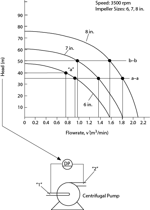
Figure E19.20 Illustration of Example 19.20

If the storage tank is located at an elevation of 35 m above the pump, predict the flow using each impeller.
If the storage tank is located at an elevation of 50 m above the pump, predict the flow using each impeller.

Solution

Figure E19.20 shows the pump curves for three different impeller sizes for the same pump. From Figure E19.20, at Δh_p = 35 m (see line a-a):

6- in Impeller: Flow = 0.93 m³/min

7- in Impeller: Flow = 1.38 m³/min

8- in Impeller: Flow = 1.81 m³/min

Therefore, each impeller can be used, and the larger impeller provides a larger flowrate.
From Figure E19.20, at Δh_p = 50 m (see line b-b):

6- in Impeller: Flow = 0 m³/min

7- in Impeller: Flow = 0.99 m³/min

8- in Impeller: Flow = 1.58 m³/min

In this case, the 6-in impeller is not sufficient to provide the desired flowrate, so only the 7-in and 8-in impellers are appropriate choices.

$\begin{matrix} - Δ h_{p} = 50 m = (P_{1} - P_{2}) / ρ g = P_{1} / ρ g - 1.2 \times 1 0^{5} / [750 (9.81)] = P_{1} / ρ g - 16 . 3 m \\ P_{1} = (50 + 16.3) ρ g = 66.3 (750) (9.81) = 4.88 \times 1 0^{5} Pa = 4 . 88 bar \end{matrix}$

19.5.4 Compressors

19.5.4.1 Compressor Curves

The performance of centrifugal compressors is somewhat analogous to that of centrifugal pumps. A characteristic performance curve, supplied by the manufacturer, defines how the outlet pressure varies with flowrate. However, compressor behavior is far more complex than that for pumps because the fluid is compressible.

Figure 19.25 shows the performance curves for a centrifugal compressor. It is immediately observed that the y-axis is the ratio of the outlet pressure to inlet pressure. This is in contrast to pump curves, which have the difference between these two values on the y-axis. Curves for two different rotation speeds are shown. As with pump curves, curves for power and efficiency are often included but are not shown here. Unlike most pumps, the speed is often varied continuously to control the flowrate because the higher power required in a compressor makes it economical to avoid throttling the outlet as in a centrifugal pump.

A graph shows the performance curves for a Centrifugal Compressor.

Figure 19.25 Performance Curves for a Centrifugal Compressor

Centrifugal compressor curves are read just like pump curves. At a given flowrate and revolutions per minute, there is one pressure ratio. The pressure ratio decreases as flowrate increases. A unique feature of compressor behavior occurs at low flowrates. It is observed that the pressure ratio increases with decreasing flowrate, reaches a maximum, and then decreases with decreasing flowrate. The locus of maxima is called the surge line. For safety reasons, compressors are operated to the right of the surge line. The surge line is significant for the following reason. Imagine the compressor is operating at a high flowrate and the flowrate is lowered continuously, causing a higher outlet pressure. At some point, the surge line is crossed, lowering the pressure ratio. This means that downstream fluid is at a higher pressure than upstream fluid, causing a backflow. These flow irregularities can severely damage the compressor mechanism, even causing the compressor to vibrate or surge (hence the origin of the term). Severe surging has been known to cause compressors to become detached from the supports keeping them stationary and literally to fly apart, causing great damage. Therefore, the surge line is considered a limiting operating condition below which operation is prohibited. Surge control on compressors is usually achieved by opening a bypass valve on a line connecting the outlet to the inlet of the compressor. When the surge point is approached, the bypass valve is opened, and gas flows from the outlet to the inlet, thereby increasing the flow through the compressor and moving it away from the surge condition.

Positive-displacement compressors also exist and are used to compress low volumes to high pressures. Centrifugal compressors are used to compress higher volumes to moderate pressures and are often staged to obtain higher pressures. Figure 19.5 illustrates the inner workings of a compressor.

19.5.4.2 Compressor Staging

There are two limiting cases for compressor behavior: isothermal and isentropic. An actual compressor is neither isothermal nor isentropic; however, the behavior lies between these two limiting cases. From the general mechanical energy balance, compressor work is

$\begin{matrix} η_{c} W_{s} = \int_{P_{_{1}}}^{P_{_{2}}} \frac{dP}{ρ} \end{matrix} (19.73)$

where subscripts 1 and 2 denote compressor inlet and outlet, respectively. For the isothermal case, assuming ideal gas behavior (which will fail as the pressure increases but is sufficient to illustrate the basic concepts),

$\begin{matrix} η_{c} W_{s, isoth} = \int_{P_{_{1}}}^{P_{_{2}}} \frac{dP}{ρ} = \frac{RT}{M} \int_{P_{_{1}}}^{P_{_{2}}} \frac{dP}{ρ} = \frac{RT}{M} \ln (\frac{P_{2}}{P_{1}}) \end{matrix} (19.74)$

For isentropic compression, the relationship from thermodynamics for adiabatic, reversible, compression is

$\begin{matrix} {PV}^{γ} = \frac{P}{ρ^{γ}} = constant \end{matrix} (19.75)$

where γ = C_p/C_v, the ratio of the constant pressure and constant volume heat capacities. Using the compressor inlet as a reference point,

$\begin{matrix} \frac{P_{1}}{ρ_{1}^{γ}} = \frac{P}{ρ^{γ}} \end{matrix} (19.76)$

Solving Equation (19.76) for ρ, using that value in Equation (19.73), and integrating yields a well-known expression from thermodynamics for adiabatic, reversible, compression of an ideal gas:

$\begin{matrix} η_{c} W_{s, isen} = \frac{γ R T_{1}}{M (γ - 1)} [{(\frac{P_{2}}{P_{1}})}^{\frac{γ - 1}{γ}} - 1] \end{matrix} (19.77)$

Taking the ratio of Equations (19.74) and (19.77), and realizing that T = T₁ in Equation (19.74), since the temperature is constant at the inlet value in the isothermal case, yields

$\begin{matrix} \frac{W_{s, isoth}}{W_{s, isen}} = \frac{\ln (\frac{P_{2}}{P_{1}})}{\frac{γ}{γ - 1} [{(\frac{P_{2}}{P_{1}})}^{\frac{γ}{γ - 1}} - 1]} \end{matrix} (19.78)$

Figure 19.26 is a plot of Equation (19.78), with the dependent variable as the compression ratio, P₂/P₁. Figure 19.26 demonstrates that the reversible, adiabatic work for isothermal compression is always less than that for isentropic compression. As the compression ratio exceeds 3 to 4, the isothermal work is significantly less than the isentropic work, making isothermal compression desirable. Of course, since compressing a gas always increases the gas temperature, isothermal compression cannot be accomplished. However, isothermal compression can be approached by staging compressors with intercooling, as illustrated in Figure 19.27 for a two-stage configuration. Isothermal compression can be reached theoretically with an infinite number of compressors each with an infinitesimal temperature rise, hardly a practical situation. From thermodynamics, it can be shown that the minimum compressor work for staged adiabatic compressors, with interstage cooling to the feed temperature to the first compressor, is accomplished with an equal compression ratio in each compressor stage. This is not necessarily the economic optimum, which would require analysis of the capital cost of the compressor stages and heat exchangers, the operating cost of the compressor, and the utility cost of the cooling medium. However, the preceding analysis explains why compressors are usually staged when the compression ratio exceeds 3 to 4.

A graph shows the comparison of isothermal and isentropic work for compressors.

Figure 19.26 Comparison of Isothermal and Isentropic Work for Compressors

A figure shows an example of a two-stage compressor configuration.

Figure 19.27 Example of Two−Stage Compressor Configuration

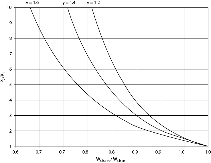
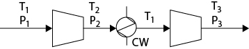
19.5.5 Performance of the Feed Section to a Process

A common feature of chemical processes is the mixing of reactant feeds before they enter a reactor. When two streams mix, they are at the same pressure. The consequences of this are illustrated by the following scenario.

Phthalic anhydride can be produced by reacting naphthalene and oxygen. The feed section to a phthalic anhydride process is shown in Figure 19.28. The mixed feed enters a fluidized bed reactor operating at five times the minimum fluidization velocity. A stream table is given in Table 19.4. It is assumed that all frictional pressure losses are associated with equipment and that frictional losses in the piping are negligible. It is temporarily necessary to scale down production by 50%. The engineer must determine how to scale down the process and to determine the new flows and pressures.

A figure shows the feed section of the Phthalic Anhydride Process.

Figure 19.28 Feed Section to Phthalic Anhydride Process

Table 19.4 Partial Stream Table for Feed Section in Figure 19.27

	Stream
	1	2	3	4	5	6	7	8
P (kPa)	80.00	101.33	343.0	268.0	243.0	243.0	243.0	200.0
Phase	L	V	L	V	V	V	V	V
Naphthalene (Mg/h)	12.82	—	12.82	—	12.82	—	12.82	12.82
Air (Mg/h)	—	151.47	—	151.47	—	151.47	151.47	151.47

It is necessary to have pump and compressor curves in order to do the required calculations. In this example, equations for the pump curves are used. These equations can be obtained by fitting a polynomial to the curves provided by pump manufacturers. As discussed in Section 19.5.3, pump curves are usually expressed as pressure head versus volumetric flowrate so that they can be used for a liquid of any density. In this example, pressure head and volumetric flowrate have been converted to absolute pressure and mass flowrate using the density of the fluids involved. Pump P-201 operates at only one speed, and an equation for the pump curve is

$\begin{matrix} Δ P (kPa) = 500 + 4.663 \dot{m} - 1.805 {\dot{m}}^{2} \dot{m} \leq 16 .00 Mg / h \end{matrix} (19.79)$

Compressor C-201 operates at only one speed, and the equation for the compressor curve is

$\begin{matrix} \begin{matrix} \frac{P_{out}}{P_{in}} = 5.201 + 2.662 \times 10^{- 3} \dot{m} - 1.358 \times 10^{- 4} {\dot{m}}^{2} \\ \begin{matrix} + 4.506 \times 10^{- 8} {\dot{m}}^{3} & \dot{m} \leq 200 Mg / h \end{matrix} \end{matrix} \end{matrix} (19.80)$

From Figure 19.27, it is seen that there is only one valve in the feed section, after the mixing point. Therefore, the only way to reduce the production of phthalic anhydride is to close the valve to the point at which the naphthalene feed is reduced by 50%. Example 19.21 illustrates the consequences of reducing the naphthalene feed rate by 50%.

Example 19.21

For a reduction in naphthalene feed by 50%, determine the pressures and flows of all streams after the scale-down.

Solution

Because it is known that the flowrate of naphthalene has been reduced by 50%, the new outlet pressure from P-201 can be calculated from Equation (19.79). The feed pressure remains at 80 kPa. At a naphthalene flow of 6.41 Mg/h, Equation (19.79) gives a pressure increase of 455.73 kPa, so P₃ = 535.73 kPa. Because the flowrate has decreased by a factor of 2, the pressure drop in the fired heater decreases by a factor of 4, since $Δ P \propto L_{eq} {\dot{v}}^{2}$ . Therefore, P₅ = 510.73 kPa. Consequently, the pressure of Stream 6 must be 510.73 kPa. The flowrate of air can now be calculated from the compressor curve equation.

The compressor curve equation has two unknowns: the compressor outlet pressure and the mass flowrate. Therefore, a second equation is needed. The second equation is obtained from a base-case ratio for the pressure drop across the heat exchanger. The two equations are

$\begin{matrix} \frac{P_{4}}{101.33} = 5.201 + 2.662 \times 10^{- 3} {\dot{m}}_{2, new}^{2} - 1.358 \times 10^{- 4} {\dot{m}}_{2, new}^{2} + 4.506 \times 10^{- 8} {\dot{m}}_{2, new}^{2} & (E19.21a) \end{matrix}$

$\begin{matrix} P_{4} - 510.73 = 25 {(\frac{{\dot{m}}_{2, new}}{151.47})}^{2} & (E19.21b) \end{matrix}$

The solution is

$\begin{array}{l} P_{4} = 512 . 84 kPa \\ {\dot{m}}_{2} = 43.80 Mg / h \end{array}$

The stream table for the scaled-down case is given in Table E19.21. Although it is not precisely true, for lack of additional information, it has been assumed that the pressure of Stream 8 remains constant.

Table E19.21 Partial Stream Table for Scaled-Down Feed Section in Figure 19.28

	Stream
	1	2	3	4	5	6	7	8
P (kPa)	80.0	101.33	535.73	512.84	510.73	510.73	510.73	200.00
Phase	L	V	L	V	V	V	V	V
Naphthalene (Mg/h)	6.41	—	6.41	—	6.41	—	6.41	6.41
Air (Mg/h)	—	43.80	—	43.80	—	43.80	43.80	43.80

It is observed that the flowrate of air is reduced by far more than 50% in the scaled-down case. This is because of the combination of the compressor curve and the new pressure of Streams 5 and 6 after the naphthalene flowrate is scaled down by 50%. The total flowrate of Stream 8 is now 50.21 Mg/h, which is 30.6% of the original flowrate to the reactor. Given that the reactor was operating at five times minimum fluidization, the reactor is now in danger of not being fluidized adequately. Because the phthalic anhydride reaction is very exothermic, a loss of fluidization could result in poor heat transfer, which might result in a runaway reaction. The conclusion is that it is not recommended to operate at these scaled-down conditions.

The question is how the air flowrate can be scaled down by 50% to maintain the same ratio of naphthalene to air as in the original case. The answer is in valve placement. Because of the requirement that the pressures at the mixing point be equal, with only one valve after the mixing point, there is only one possible flowrate of air corresponding to a 50% reduction in naphthalene flow-rate. Effectively, there is no control of the air flowrate. A chemical process would not be designed as in Figure 19.28. The most common design is illustrated in Figure E19.21. With valves in both feed streams, the flowrates of each stream can be controlled independently.

A figure shows the feed section of the Phthalic Anhydride Process, with a better valve placement.

Figure E19.21 Feed Section to Phthalic Anhydride Process with Better Valve Placement Than Shown in Figure 19.28

WHAT YOU SHOULD HAVE LEARNED

How to write the mass balance for pipe flow
How to apply the mechanical energy balance to pipe flow
How to apply the force balance to flow around submerged objects
The types of pipes and pipe sizing
The types of pumps and compressors and their applicability
The purpose of including valves in a piping system
How to design and analyze performance of a system for frictional flow of fluid in pipes
How to design a system for frictional flow of fluid with submerged objects such as packed and fluidized beds
Methods for flow measurement
How to analyze existing fluid flow equipment
What net positive suction head is and the limitations it places on piping system design
How to analyze pump and system curves to understand the limitations of pumps
Why compressors are staged

References

1. Geankoplis, C., Transport Processes and Separation Process Principles, 4th ed. (Upper Saddle River, NJ: Prentice Hall, 2003), 99–100.

2. Perry, R. H., and D. Green, Perry’s Chemical Engineers’ Handbook, 6th ed. (New York: McGraw-Hill, 1984), Section 5.

3. Couper, J. R., W. R. Penney, J. R. Fair, and S. M. Walas, Chemical Process Equipment: Selection and Design, 3rd ed. (New York: Elsevier, 2012), ch. 7.

4. Green, D. W., and R. H. Perry., Perry’s Chemical Engineers’ Handbook, 8th ed. (New York: McGraw-Hill, 2008), Section 10.

5. McCabe, W. L., J. C. Smith, and P. Harriott, Unit Operations of Chemical Engineering, 5th ed. (New York: McGraw-Hill, 1993).

6. Bird, R. B., W. E. Stewart, and E. N. Lightfoot, Transport Phenomena, 2nd ed. rev. (New York: Wiley, 2006), 51.

7. Pavlov, K. F., P. G. Romankov, and A. A. Noskov, Problems and Examples for a Course in Basic Operations and Equipment in Chemical Technology (Moscow: MIR, translated, 1981).

8. Levenspiel, O., Engineering Flow and Heat Exchange, 3rd ed. (New York: Springer, 2014), 27.

9. Darby, R., Chemical Engineering Fluid Mechanics, 2nd ed. (New York: Marcel Dekker, 2001), 209.

10. Kittredge, C. P., and D. S. Rowley. “Resistance Coefficients for Laminar and Turbulent Flow Through One-Half-Inch Valves and Fittings,” Trans. ASME 79 (1957): 1759–1766.

11. Haider, A., and O. Levenspiel, “Drag Coefficient and Terminal Velocity of Spheres and Nonspherical Particles,” Powder Technol. 58 (1989): 63–70.

12. Wen, C. Y., and Y.-H. Yu, “A Generalized Method for Predicting the Minimum Fluidization Velocity,” AIChE J. 12 (1966): 610–612.

13. Kunii, D., and O. Levenspiel, Fluidization Engineering, 2nd ed. (Stoneham, MA: ButterworthHeinemann, 1991).

14. Miller, R.W., Flow Measurement Engineering Handbook (New York: McGraw-Hill, 1983).

15. Cheremisinoff, N. P., and P. N. Cheremisinoff, Instrumentation for Process Flow Engineering (Lancaster: Technomic, 1987).

16. Walas, S., Chemical Process Equipment: Selection and Design (Stoneham, MA: Butterworth, 1988).

Short Answer Questions

1. Explain the physical meaning of each term in the mechanical energy balance.

2. luid flows from a larger-diameter pipe to a smaller-diameter pipe. How does the velocity change?

3. Explain the concept of pressure head.

4. luid flows downward in a vertical pipe of uniform diameter. How does the velocity change with position?

5. liquid flows vertically downward through a pipe of uniform diameter at steady state. Explain how the mass flowrate, volumetric flowrate, and velocity change with vertical position.

6. Explain the meaning of the Reynolds number in terms of forces.

7. Sketch the approximate shape of a graph of frictional losses versus Reynolds number. Discuss two other situations in which the graph has similar shape.

8. There are three key parameters that affect frictional loss in pipe flow. State two of them and explain the effect (i.e., whether the parameter increases or decreases, how the frictional loss is affected).

9. For sections of pipes in series, what is the relationship between the mass flowrate in each section? What is the relationship between the pressure drops in each section?

10. For sections of pipes in parallel, what is the relationship between the mass flowrate in each section? What is the relationship between the pressure drops in each section?

11. How is the mechanical energy balance different for compressible flow compared to incompressible flow?

12. What is the difference between form drag and frictional drag?

13. Define void fraction.

14. Explain the difference between void volume, solid volume, and total volume.

15. Define sphericity.

16. When is mercury a better manometer fluid than water or oil? When is mercury not recommended? Assume the specific gravity of mercury is 13.2, and the specific gravity of oil is 0.8.

17. Explain the physical meaning of the intersection of the NPSH_R and NPSH_A curves.

18. Explain the physical meaning of the intersection of the pump and system curves.

19. Why does a compressor cost more to operate than a pump?

20. Why are compressors often staged with intercooling?

21. For fully developed turbulent flow, assuming all variables not mentioned are held constant:

What is the effect of doubling the flowrate on the pressure drop?
What is the effect of increasing the pipe diameter by 25% on pressure drop?
What is the effect of increasing the pipe diameter on flowrate?
What is the effect of increasing pipe length on pressure drop?
What is the effect of increasing pipe length on flowrate?
What is the effect on pressure drop of replacing one long pipe segment with two equal-sized pipe segments of half the length placed in parallel?

22. Repeat Problem 19.21 for laminar flow.

Problems

23. Consider the situation depicted in Figure P19.23. The fluid is an oil with a specific gravity of 0.85. Fill in the missing data in Table P19.23.

A figure shows streams 1 and 2 combining initially. The stream thus produced splits to streams 3 and 4.

Figure P19.23

Table P19.23

Stream	Pipe	$\dot{m}$ (kg/s)	$\dot{v}$ (m3/s)	u (m/s)
1	2-in, schedule 40	6
2	3.5-in, schedule 40		0.0106
3	1.5-in, schedule 40			4.032
4	3-in, schedule 40

24. For water flowing in the situation shown in Figure P19.24 and the data in Table P19.24, do the following:

Calculate the mass flowrate of Stream 3.
Calculate the velocity of Stream 4.
What schedule-40 pipe size must be used in Stream 3?

Figure P19.24

Table P19.24

Stream	Pipe	u (m/s)
1	1-in, schedule 40	5
2	1.5-in, schedule 40	3
3	?-in, schedule 40	2.18
4	4-in, schedule 40	?

25. Consider the situation depicted in Figure P19.25. The liquid level in the cylindrical tank is increasing at 0.02 ft/sec.

What is the net rate of flow into the tank?
What is the velocity in the 3-in pipe?

A figure shows a tank filled with water with one inlet and two outlets of varying dimensions.

Figure P19.25

26. Water is pumped through a 750-ft length of 6-in, schedule-40 pipe. The discharge at the end of the pipe is 50 ft above the suction end. The pump is 80% efficient and is driven by a 20 hp motor. If the friction loss in the pipe is 50 ft lb_f/lb, what is the flowrate through the pipe?

27. A hydroelectric power plant takes 25 m³/s of water from a large reservoir through its turbine and discharges it to the atmosphere at 1 m/s. The turbine is 50 m below the reservoir surface. The frictional head loss in the system is 10 m. The turbine and electric generator as a whole are 80% efficient. Assuming turbulent flow, calculate the power extracted by the turbine.

28. Water is pumped at a constant rate of 10 m³/h from an open tank on the floor to an open tank with a level 10 m above the floor. Frictional losses in the 50-mm-diameter pipe between the tanks are 3.5 J/kg. At what height above the floor must the water level be kept if the pump can develop only 0.1 kW? The pump is 75% efficient.

29. Water in a dam on a 75-ft-deep river is passed through a turbine to produce energy. The outlet of the turbine is 15 ft above the river bed. The mass flowrate of water is 65,000 lb/s, and the inside diameter of the discharge pipe is 10 ft. Discharge is to the atmosphere, and frictional losses may be neglected. For a 55% efficient turbine, calculate the power produced.

30. Many potential drugs have low water solubility, hindering their transport in the body’s aqueous material distribution medium (blood). One way to improve solubility is to decrease particle size below 1 μm diameter. One method to do this is by high-pressure homogenization, using a homogenizer, which is basically a nozzle. In this process, the drug is dispersed in a solvent and forced through a narrow orifice (nozzle) at high pressure. As the liquid enters the orifice, it experiences a pressure drop so great it partially vaporizes. As it exits the constriction, the vapor bubbles collapse violently and produce local disturbances, breaking up the surrounding solid particles.

A high-pressure homogenizer is being used to decrease the size of some drug particles. The particles are suspended in water at 25°C and sent through the homogenizer at 250 mL/min. The pressure before the orifice is 34.5 MPa, and the diameter of the pipe is 0.1 m. Determine the diameter orifice (nozzle) that results in an exit pressure at the vapor pressure of water. Neglect friction.

31. A pump operating at 80% efficiency delivers 30 gal/min of water from a reservoir to an open-air storage tank at a chemical plant 1 mi away. A 3-in, schedule-40 pipe is used, and the frictional losses are 200 ft lb_f/lb. The elevation of the liquid level in the tank is 873 ft above sea level, and the elevation of the liquid level in the reservoir is 928 ft above sea level.

What is the minimum horsepower required for the pump?
The elevation of the reservoir is fixed. What elevation of the liquid level of the tank would make the pump unnecessary?

32. A pressurized tank situated above ground level contains a liquid with specific gravity of 0.9. The liquid flows down to ground level through 4-in, schedule-40 pipe through a pump (75% efficiency) and into a tank at a level 25 m above the level of the source tank at a pressure of 550 kPa through 2-in, schedule-40 pipe. The pump power is 6.71 kW. A pressure gauge at the pump entrance reads 115.6 kPa, and a pressure gauge at the pump discharge reads 762.6 kPa. The frictional losses in the piping on the suction side of the pump and on the discharge side of the pump are 30 J/kg and 50 J/kg, respectively.

What is the mass flowrate of liquid through the system?
What is the velocity in the 2-in, schedule-40 pipe?
What is the pressure of the liquid in the source tank?
Determine whether the kinetic energy contribution to the mechanical energy balance is small.

33. Water is pumped from one storage tank to a higher tank at a steady rate of 10^-3m³/s. The difference in the elevations of the two water tanks is 50 m. The storage tank, which serves a source, is open to the atmosphere, while the tank receiving the water has a pressure of 170.3 kPa. Pressure gauges in the pipeline at the inlet and outlet of the pump read 34.5 kPa and 551.6 kPa, respectively. The power supplied by an electric motor to the pump shaft is 1000 W. All piping is 1-in, schedule-40 steel pipe. Find the pump efficiency and friction loss in the pipe per kg of water.

34. Oil (SG = 0.88) flows at 5 ft³/s from one tank, through a pump, to another tank. The pipe diameter between the source tank and the pump is 12 in, and the pipe diameter between the pump and the destination tank is 6 in. The liquid level in the source tank is 10 ft above the pump, which is at ground level. The liquid level in the destination tank is 12 ft. The source tank is at 25 psia, and the destination tank is open to the atmosphere. A manometer is connected to the upstream and downstream pipes, immediately adjacent to the pump, with a differential height of 36 in of mercury. The pump is 75% efficient. Frictional losses may be neglected.

What is the power rating of the pump?
What is the maximum possible height of the bottom of the destination tank?

35. A fluid with specific gravity of 0.8 is in a tank, at a pressure of 150 kPa, with a level maintained at 5 m above ground level. The fluid leaves the tank through 4-in, schedule-40 pipe (frictional loss of 30 J/kg) at a mass flowrate of 6.5 kg/s and enters a pump at ground level. The pump power is 1.5 kW and is 70% efficient. The fluid leaving the pump flows through 3.5-in, schedule-40 pipe (frictional loss of 50 J/kg) to a “final” point in the pipe above the original tank level, where the pressure is 200 kPa.

Find the velocity at the final point in the pipe.
Determine the pressure at the pump inlet.
Determine the height above the ground of the final point in the pipe.

36. Consider the problem of how long it takes for a tank to drain. Consider an open-top cylindrical tank with one horizontal exit pipe at the bottom of the tank that discharges to the atmosphere. The tank has a diameter, d, and the height of liquid in the tank at any time is h.

The mass balance is unsteady state. Explain why the mass balance is

$\frac{dm}{dt} = - {\dot{m}}_{out}$

where m is the mass of liquid in the tank and ${\dot{m}}_{out}$ is the mass flowrate out of the tank.
The mass in the tank is the fluid density times the volume of liquid in the tank. The flowrate, ${\dot{m}}_{out}$ , can be related to the velocity and the cross-sectional area of the exit pipe based on what we have already learned. The volume of liquid in the tank can be related to the height of liquid in the tank. Simplify the differential mass balance to obtain an expression for the height of liquid in the tank as a function of the velocity of the liquid through the exit pipe.
Now, write a mechanical energy balance on the fluid in the tank and pipe from the top level in the tank to the pipe outlet, neglecting friction. It is generally assumed the velocity of the tank level (i.e., the fluid level in the tank) is small because of the large diameter. Solve for the velocity, and rearrange the differential equation to look like

$\frac{dh}{dt} = af (h)$

where a is a group of constants and f(h) is a function of the height that you have derived.
Solve this differential equation for height as a function of time with the initial condition of a height of h_o at time zero.
Rearrange the answer to Part (d) to get an expression for the time for complete drainage.

37. The following equations describe a fluid-flow system. Draw and label the system.

$\begin{array}{l} {\dot{m}}_{1} + {\dot{m}}_{2} = {\dot{m}}_{3} = {\dot{m}}_{4} \\ \frac{P_{4} - P_{3}}{ρ} + \frac{v_{4}^{2} - v_{3}^{2}}{2} - η W_{s} = 0 \\ \frac{P_{5} - P_{4}}{ρ} - \frac{v_{4}^{2}}{2} + g (z_{5} - z_{4}) + e_{f} = 0 \end{array}$

38. The following equations describe a fluid flow system, with friction neglected. Draw and label the system, making sure that your diagram is visually accurate.

$\begin{array}{l} {\dot{m}}_{3} + {\dot{m}}_{2} = {\dot{m}}_{4} = {\dot{m}}_{5} \\ \frac{P_{2} - P_{1}}{ρ} + g (z_{2} - z_{1}) + \frac{v_{2}^{2}}{2} = 0 \\ g (z_{6} - z_{1}) - η W_{s} = 0 \\ \frac{P_{5} - P_{4}}{ρ} + \frac{v_{5}^{2} - v_{4}^{2}}{ρ} - η W_{s} = 0 \\ \frac{P_{6} - P_{5}}{ρ} + g (z_{6} - z_{5}) - \frac{v_{5}^{2}}{2} = 0 \\ z_{6} > z_{1} \end{array}$

39. An aneurysm is a weakening of the walls of an artery causing a ballooning of the arterial wall. The result is a region of larger diameter than a normal artery. If the “balloon” ruptures in a high-blood-flow area, such as the aorta, death is almost instantaneous. Fortunately, there are often symptoms due to slow leakage that can precede rupture. What happens to the blood velocity as it passes through the aneurysm? Justify your answer using equations. In the human body, very small changes in pressure can be significant. Using the mechanical energy balance, neglecting only friction and potential energy effects, analyze the pressure change as blood enters the aneurysm a large distance from the heart, so that the pulse flow is not an issue. The blood is flowing in a region not in the vicinity of the heart. What is the effect of the observed pressure change?

40. A pipeline is replaced by new 2-in, schedule-40, commercial-steel pipe. What power would be required to pump water at a rate of 100 gpm through 6000 ft of this pipe?

41. Hot water at 43°C flows from a constant-level tank through 2-in, schedule-40, commercial-steel pipe, from which it emerges 12.2 m below the level in the tank. The equivalent length of the piping system is 45.1 m. Calculate the rate of flow in m³/s.

42. Crude oil (μ = 40 cP, SG = 0.87) is to be pumped from a storage tank to a refinery through a series of pump stations via 10-in, schedule-20, commercial-steel pipeline at a flowrate of 2000 gpm. The pipeline is 50 mi long and contains 35 90° elbows and 10 open gate valves. The pipeline exit is 150 ft higher than the entrance, and the exit pressure is 25 psig. What horsepower is required to drive the pumps if they are 70% efficient?

43. A pipeline to carry 1 million bbl/day of crude oil (1 bbl = 42 gal, SG = 0.9, μ = 25 cP) is constructed with 50-in-inside-diameter, commercial-steel pipe and is 700 mi long. The source and destination are at atmospheric pressure and the same elevation. There are 50 wide-open gate valves, 25 half-open globe valves, and 50 45° elbows. There will be 25 identical pumps along this pipeline, each with an efficiency of 70%. What is the power required for each pump?

44. A pump draws a solution of specific gravity 1.2 with the viscosity of water from a ground-level storage tank at 50 psia through 3.5-in, schedule-40, commercial-steel pipe at a rate of 12 lb/s. The pump produces 4.5 hp with an efficiency of 75%. The pump discharges through a 2.5-in, schedule-40 commercial steel pipe to an overhead tank at 100 psia, which is 50 ft above the level of solution in the feed tank. The suction line has an equivalent length of 20 ft, including the tank exit. The discharge line contains a half-open globe valve, two wide-open gate valves, and two 90° elbows. What is the maximum total length of discharge piping allowed for this pump to work?

45. Many chemical plants store fuel oil in a “tank farm” on the outskirts of the plant. To prevent an environmental disaster, there are specific rules regarding the design of such facilities. One such rule is that there be an emergency dump tank with the capacity of the largest storage tank. Should a leak or structural problem occur with a tank, the fuel oil can be pumped into the emergency dump tank.

Consider the design of the pumping system from a 250 m³ tank storing #6 fuel oil into a 250 m³ dump tank. The viscosity of #6 fuel oil is 0.8 kg/m s, and its density is 999.5 kg/m³. The piping system consists of 43 m of commercial-steel pipe, four 90° flanged regular elbows, a sharp entrance, an exit, and a pump. The oil must be pumped to an elevation 3.35 m above the exit point from the source tank.

If 20-in, schedule-40, commercial-steel pipe is used, and if it is necessary to accomplish the transfer within 45 min, determine the power rating required of the pump. Assume the pump is 80% efficient.
If the pump to be used has 10 kW at 80% efficiency, and the pipe is 20-in, schedule-40, commercial-steel pipe, determine how long the transfer will take.
If the pump to be used has 20 kW at 80% efficiency, and the transfer is to be accomplished in 45 min, determine the required schedule-40 pipe size.

46. Two parallel sections of pipe branch from the same split point. Both branches end at the same pressure and the same elevation. Branch 1 is 3-in, schedule-40, commercial-steel pipe and has an equivalent length of 12 m. Branch 2 is 2-in, schedule-80, commercial-steel pipe and has an equivalent length of 9 m.

Assuming fully turbulent flow, what is the split ratio between the two branches?
Suppose that Branch 2 ends 5 m higher than Branch 1. What is the split ratio between the branches in this case?

47. Consider a two-pipes-in-series system: that is, Pipe 1 is followed by Pipe 2. The liquid is water at room temperature with a mass flowrate of 2 kg/s. The pipes are horizontal. Calculate the pressure drop across these two pipes and the power necessary to overcome the frictional loss. Ignore the minor losses due to the pipe fitting. The pipe data are

Pipe	L (m)	Pipe Size	Material
1	10	1-in, schedule-40	Commercial steel
2	15	2-in, schedule-40	Cast iron

48. Assume that the same two pipes in Problem 19.47 are now in parallel with the same total pressure drop. Compute the mass flowrate in each section of pipe. Neglect additional frictional losses due to the parallel piping. Explain the reason for the observed split between the parallel pipes.

49. A pipe system to pump #6 fuel oil (μ = 0.8 kg/m s, ρ = 999.5 kg/m³) consists of 50 m of 8-in, schedule-40, commercial-steel pipe. It has been observed that the pressure drop is 8.79 × 10⁴ Pa.

Determine the volumetric flowrate of the fuel oil.
Extra capacity is needed. Therefore, it has been decided to add a parallel line of the same length (neglect minor losses) using 5-in, schedule-40, commercial-steel pipe. By what factor will the fuel oil volumetric flowrate increase?

50. There are three equal-length sections of identical 3-in, schedule-40, commercial-steel pipe in series. An increased flowrate of 20% is needed. How is the pressure drop affected? It is decided to replace the second section with two equal-length, identical sections of the original pipe in parallel. How is the pressure drop in this system affected relative to the original case? Neglect minor losses due to elbows and fittings and assume fully developed turbulent flow.

51. Consider two parallel arteries of the same length, both fed by a main artery. The flowrate in the main artery is 10^-6 m³/s. One branch is stenotic (has plaque build-up due to too many Big Macs, Double Whoppers, etc.). The stenotic artery will be modeled as a rigid pipe with 60% the diameter of the healthy artery (diameter of 0.1 cm). For this problem, blood may be considered to be a Newtonian fluid with the properties of water. What fraction of the blood flows in each arterial branch? Be sure to validate any assumptions made.

52. One of the potential benefits of the production of shale gas is that certain seams of the gas contain significant amounts of ethane, which can be cracked into ethylene, a building block for many other common chemicals (polyethylene, ethylene oxide, which is made into ethylene glycol among many others, and tetrafluoroethylene, the monomer for Teflon). Assume that a cracker plant produces ethylene (C₂H₄) at 5 atm and 70°F. It is to be delivered by pipeline to a neighboring plant, which was built near the ethylene cracker facility, which is 10 miles away. The pressure at the neighboring plant entrance must be 2.5 atm. It has been suggested that 6-in, schedule-40, commercial-steel pipe be used. What delivery mass flowrate is possible with this pipe size? If you need to make an assumption, do so and prove its validity.

53. Natural gas (methane, μ = 10^-5 kg/m s) must flow in a pipeline between compression stations. The compressor inlet pressure is 250 kPa, and its outlet pressure is 1000 kPa. Assume isothermal flow at 25°C. The pipe is 6-in, schedule-40, commercial steel. The mass flowrate is 2 kg/s. What is the required distance between pumping stations?

54. Your plant produces ethylene at 6 atm and 60°F. It is to be delivered to a neighboring plant 5 miles away via pipeline, and the pressure at the neighboring plant entrance must be 2 atm. The contracted delivery flowrate is 2 lb/sec. It has been suggested that 4-in, schedule-40, commercial-steel pipe be used. Evaluate this suggestion. Be sure to validate any assumptions made.

55. Calculate the terminal velocity of a 2 mm diameter lead sphere (SG = 11.3) dropped in air. The properties of air are ρ = 1.22 kg/m³ and μ = 1.81 × 10^-5 kg/m s.

56. A packed bed is composed of crushed rock with a density of 200 lb/ft³ with an assumed particle diameter of 0.15 in. The bed is 8 ft deep, has a porosity of 0.3, and is covered by a 3 ft layer of water that drains by gravity through the bed. Calculate the velocity of water through the bed, assuming the water enters and exits at 1 atm pressure.

57. A hollow steel sphere, 5 mm in diameter with a mass of 0.05 g, is released in a column of liquid and attains an upward terminal velocity of 0.005 m/s. The liquid density is 900 kg/m³, and the sphere is far enough from the container walls so that their effect may be neglected. Determine the viscosity of the liquid in kg/m s. Hint: Assume Stokes flow and confirm the assumption with your answer.

58. In a particular sedimentation vessel, small particles (SG = 1.1) are settling in water at 25°C. The particles have a diameter of 0.1 mm. What is the terminal velocity of the particles? Validate any assumptions made.

59. At West Virginia University, each Halloween, there is a pumpkin-drop contest. College, high-school, and middle-school students participate. The goal is to drop a pumpkin off the top of the main engineering building (assume about 100 ft) and have it land close to a target without being damaged. Packing and parachutes are commonly used. You have a theory that the terminal velocity at which a pumpkin packed in your newly invented, proprietary bubble wrap can hit the ground and remain intact is 50 m/s. You will use no parachute, and the shape will be approximately spherical. The pumpkin plus wrapping has a diameter of 40 cm. By calculating the actual terminal velocity, determine whether the pumpkin will exceed the desired terminal velocity. Assume that the wrapped pumpkin has the specific gravity of water, and assume the air is at 25°C and 1 atm.

60. Air enters and passes up through a packed bed of solids 1 m in height. Using the data provided, what are the pressure drop and the outlet pressure?

Data:

$\begin{array}{l} v_{s} = 1 m / s & P_{inlet} = 0.2 MPa \\ T = 293 K & μ = 1.8 \times 10^{- 5} kg/m/s \\ D_{p} = 1 mm & ε = 0.4 \\ ρ_{s} = 9500 kg / m^{3} \end{array}$

61. In the regeneration of a packed bed of ion-exchange resin, hydrochloric acid (SG = 1.2, μ = 0.002 kg/m s) flows upward through a bed of resin particles (particle density of 2500 kg/m³). The bed is 40 cm in diameter, and the particles are spherical with a diameter of 2 mm and a bed void fraction of 0.4. The bed is 2 m deep, and the bottom of the bed is 2 m off the ground. The acid is pumped at a rate of 2 ×10^-5 m³/s from an atmospheric pressure, ground-level storage tank through the packed bed and into another atmospheric pressure, ground-level storage tank, in which the filled height is 2 m. The complete piping system consists of 75 equivalent meters of 4-in, schedule-40, commercial-steel pipe.

Determine the required power of a 75% efficient pump for this duty. Remember that a pump must be sized for the maximum duty needed.
What do you learn from the numbers in Part (a) regarding the relative magnitudes of the maximum duty and the steady-state duty?
What is the pressure rise needed for the pump?

62. A gravity filter is made from a bed of granular particles assumed to be spherical. The bed porosity is 0.40. The bed has a diameter of 0.3 m and is 1.75 m deep. The volumetric flowrate of water at 25°C through the bed is 0.006 m³/s. What particle diameter is required to obtain this flowrate?

63. Calculate the flowrate of air at standard conditions required to fluidize a bed of sand (SG = 2.4) if the air exits the bed at 1 atm and 70°F. The sand grains have an equivalent diameter of 300 μm, and the bed is 3 ft in diameter and 1.5 ft deep, with a porosity of 0.33.

64. Consider a catalyst, specific gravity 1.75, in a bed with air flowing upward through it at 650 K and an average pressure of 1.8 atm (μ_air = 3 × 10^-5 kg/m s). The catalyst is spherical with a diameter of 0.175 mm. The static void fraction is 0.55, and the void fraction at minimum fluidization is 0.56. The slumped bed height is 3.0 m, and the fluidized bed height is 3.1 m.

Calculate the minimum fluidization velocity.
Calculate the pressure drop at minimum fluidization.
Estimate the pressure drop at one-half of the minimum fluidization velocity assuming incompressible flow.

65. A manometer containing oil with a specific gravity (SG) of 1.28 is connected across an orifice plate in a horizontal pipeline carrying seawater (SG = 1.1). If the manometer reading is 16.8 cm, what is the pressure drop across the orifice? What is it in inches of water?

66. Water is flowing downhill in a pipe that is inclined 35° to the horizontal. A mercury manometer is attached to pressure taps 3 in apart. The interface in the downstream manometer leg is 1.25 in higher than the interface in the upstream leg. What is the pressure drop between the two pressure taps?

67. An orifice having a diameter of 1 in is used to measure the flowrate of SAE 10 lube oil (SG = 0.928, μ = 60 cP) in a 2.5-in, schedule-40, commercial-steel pipe at 70°F. The pressure drop across the orifice is measured by a mercury (SG = 13.6) manometer, which reads 3 cm.

Calculate the volumetric flowrate of the oil.
How much power is required to pump the oil through the orifice (not the pipe, just the orifice)?

68. You must install a centrifugal pump to transfer a volatile liquid from a remote tank to a point in the plant 1000 ft from the tank. To minimize the distance that the power line to the pump must be strung, it is desirable to locate the pump as close as possible to the plant. If the liquid has a vapor pressure of 30 psia, the pressure in the tank is 30 psia, the level in the tank is 40 ft above the pump inlet, and the required pump NPSH is 20 ft, what is the closest that the pump can be located to the plant without the possibility of cavitation? The line is 2-in, schedule-40, commercial steel, the flowrate is 75 gpm, and the fluid properties are ρ = 45 lb/ft³ and μ = 5 cP.

69. Refer to Figure P19.69. Answer the following questions. Explain each answer.

At what flowrate is NPSHA = 3.2 m? Comment on the feasibility of operating at this flowrate.
At what flowrate does the pump produce 33.5 m of head? What is the system frictional loss at this flowrate? What is the pressure drop across the control valve at this flowrate?
At what flowrate does cavitation become a problem?
What is the maximum possible flowrate?
If the source and destination pressures are identical, what is the elevation difference between source and destination?
At a flowrate of 1 L/s, what is the system frictional head loss?
At a flowrate of 1 L/s, what head is developed by the pump?
At a flowrate of 1 L/s, what is the head loss across the control valve?

Two graphs show the volumetric flow rate of Acrylic Acid at 89 degrees Celsius.

Both graphs have a horizontal axis labeled Volumetric Flowrate of Acrylic Acid (89 degrees Celsius), liters per second, ranging from 0.0 to 3.0, in increments of 0.5. The vertical axis of the first graph is labeled Head (meters of liquid), ranging from 0 to 60, in increments of 5. The System curve begins at (0.0, 16) and curves gradually up to reach (3.0, 50). The Pump curve begins at (0.0, 35) and curves gradually down to reach (3.0, 4). The two curves meet at (1.75, 30). The vertical axis of the second graph is labeled N P S H (meters of liquid), ranging from 2.2 to 4.0, in increments of 0.2. The N P S H subscript A curve begins at (0.0, 3.5) and gradually curves down to (3.0, 2.7). The N P S H subscript R curve begins at (0.0, 2.6) and rises up to (3.0, 4.0), through the point (2.75, 3.7). The two curves intersect at (1.9, 3.15). All coordinate plots are approximate.

Figure P19.69 Volumetric Flowrate of Acrylic Acid (at 89°C), L/s

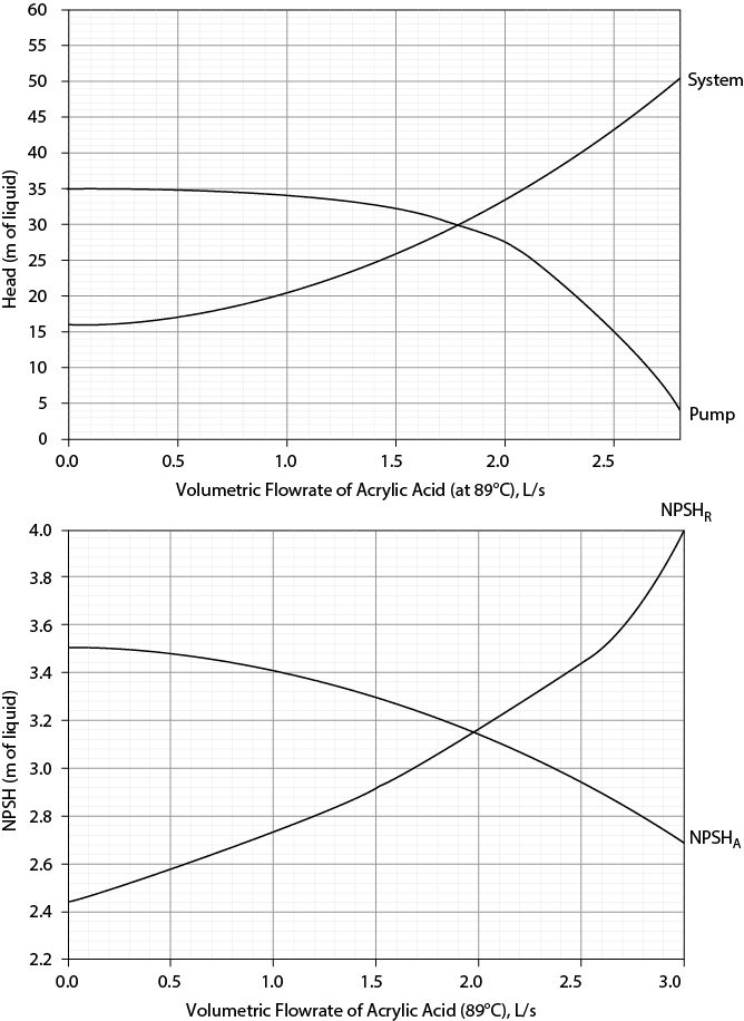
70. Benzene at atmospheric pressure and 41°C is in a tank with a fluid level of 15 ft above a pump. The pump provides a pressure increase of 50 psi to a destination 25 ft above the tank fluid level. The suction line to the pump has a length of 20 ft and is 2-in, schedule-40. The discharge line has a length of 40 ft to the destination and is 1.5-in, schedule-40. The flowrate of benzene is 9.9 lb/sec.

Derive an expression for the NPSH in head units (ft of liquid) vs. flowrate in ft³/s.
Derive an expression for the system curve in head units (ft of liquid) vs. flowrate in ft³/s.
Locate the operating point on both plots on Figure P19.70.

The first graph has the horizontal axis labeled Flow of Benzene (41 degrees Celsius), cubic feet per second, ranging from 0.0 to 0.5, in increments of 0.1, and the vertical axis labeled Pressure head across pump, feet of liquid, ranging from 0 to 1600, in increments of 200. The curve begins at (0.0, 1400), declines slightly to (0.2, 1350), where it bends downward and continues as a slant to (0.41, 200). The second graph has the horizontal axis labeled Flow of Benzene (41 degrees Celsius), cubic feet per second, ranging from 0.0 to 0.6, in increments of 0.1, and the vertical axis labeled N P S H subscript R, feet of liquid, ranging from 0 to 50, in increments of 10. The curve begins at (0.0, 5), rises slightly to (0.2, 6), where it bends upward and continues to (0.5, 30). All coordinate plots are approximate.

Figure P19.70 Flow of Benzene (at 41°C), ft³/s
What is the maximum flowrate before cavitation becomes a problem?
What is the pressure drop across the valve at the operating point?
What is the maximum flowrate possible with one pump, two pumps in series, and two pumps in parallel?

Data:

$\begin{array}{l} {log}_{10} P_{benzene}^{*} (mm Hg) = 6.90565 - \frac{1211.033}{T (° C) + 220.79} \\ ρ_{benzene} = 51.9 lb / {ft}^{3} \\ μ_{benzene} = 0.85 cP \end{array}$

71. Acrylic acid at 89°C and 0.16 kPa (ρ = 970 kg/m³, μ = 0.46 cP) leaves the bottom of a distillation column at a rate of 1.5 L/s. The bottom of a distillation column may be assumed to behave like a tank containing vapor and liquid in equilibrium at the temperature and pressure of the exit stream. The liquid must be pumped to a railroad heading supply tank 4.0 m above the liquid level in the distillation column, where the pressure must be 116 kPa. The liquid level at the bottom of the distillation column is 3.5 m above the pump suction line, and the frictional head loss for the suction line including the tank exit is 0.2 m of acrylic acid. There is a cooler after the pump with a pressure drop of 3.5 m of acrylic acid. The discharge line is 1.5-in, schedule-40, commercial-steel pipe, with an equivalent length of 200 m. The entire process may be assumed to be isothermal at 89°C. The problem at hand is whether this system can be scaled up by 20%. The plots required for this analysis are in Figure P19.71.

Based on a pump/system curve analysis, can this portion of the process be scaled up by 20%? If not, what is the maximum scale-up percentage?
Based on an NPSH analysis, is it good operating policy for this portion of the process to be scaled up by 20%? If not, what is the maximum recommended scale-up percentage?

Figure P19.71 Volumetric Flowrate of Acrylic Acid (89°C), L/s

72. Consider the pump and system curves indicated by the data in Table P19.72. Answer the following questions.

If the source and destination are at the same height, what is the pressure change from source to destination?
The operating condition is 1.2 L/s. What is ΔP_friction at this point?
At 1.2 L/s, what pressure change does the pump provide?
At 1.2 L/s, what is the pressure drop across the control valve following the pump?
What is the maximum flowrate possible with this (assumed single) pump?
What is the maximum flowrate possible with two identical pumps in series?
What is the maximum flowrate possible with two identical pumps in parallel?

Table P19.72

Pump Curve		System Curve
Pressure Developed (kPa)	Flowrate (L/s)	Pressure Change (kPa)	Flowrate (L/s)
225.0	0.00	54.0	0.00
225.0	0.40	59.0	0.50
225.0	0.80	80.0	1.00
224.0	1.20	115.0	1.50
220.0	1.50	200.0	2.00
185.0	1.86	559.0	2.50
0.0	2.60

..................Content has been hidden....................

You can't read the all page of ebook, please click here login for view all page.

Table of Contents for Chapter 19 Process Fluid Mechanics

Create new playlist

Sign In

Sign Up

Chapter 19: Process Fluid Mechanics

19.1 Basic Relationships in Fluid Mechanics

19.1.1 Mass Balance

19.1.2 Mechanical Energy Balance

19.1.3 Force Balance

19.2 Fluid Flow Equipment

19.2.1 Pipes

19.2.2 Valves

19.2.3 Pumps

19.2.4 Compressors

19.3 Frictional Pipe Flow

19.3.1 Calculating Frictional Losses

19.3.2 Incompressible Flow

19.3.2.1 Single-Pipe Systems

19.3.2.2 Multiple-Pipe Systems

19.3.3 Compressible Flow

19.3.4 Choked Flow

19.4 Other Flow Situations

19.4.1 Flow Past Submerged Objects

19.4.2 Fluidized Beds

19.4.3 Flowrate Measurement

19.5 Performance of Fluid Flow Equipment

19.5.1 Base-Case Ratios

19.5.2 Net Positive Suction Head

19.5.3 Pump and System Curves

19.5.4 Compressors

19.5.4.1 Compressor Curves

19.5.4.2 Compressor Staging

19.5.5 Performance of the Feed Section to a Process

References

Short Answer Questions

Problems

Table of Contents for
Chapter 19 Process Fluid Mechanics