Chapter 13: Synthesis of a Process Using a Simulator and Simulator Troubleshooting
WHAT YOU WILL LEARN
Process simulators are used in the design of chemical processes.
All process simulators contain the same basic algorithms and require the same information, but they all have different user interfaces.
The correct choice of thermodynamics package is crucial for accurate simulations of chemical processes.
Simulation of highly nonideal vapor-liquid equilibrium is supported by all process simulators.
Using solid components requires careful evaluation and implementation.
The advancement in computer-aided process simulation over the past generation has been nothing short of spectacular. Until the late 1970s, it was rare for a graduating chemical engineer to have any experience in using a chemical process simulator. Most material and energy balances were still done by hand by teams of engineers. The rigorous simulation of multistaged separation equipment and complicated reactors was generally unheard of, and the design of such equipment was achieved by a combination of simplified analyses, shortcut methods, and years of experience. In the present day, however, companies now expect their junior engineers to be conversant with a wide variety of computer programs, especially a process simulator.
To some extent, the knowledge base required to simulate a chemical process successfully will depend on the simulator used. Currently there are several process simulators on the market, for example, CHEMCAD, Aspen Plus, Aspen HYSYS, PRO/II, and SuperPro Designer. Many of these companies advertise their product in the trade magazines—for example, Chemical Engineering, Chemical Engineering Progress, Hydrocarbon Processing, or The Chemical Engineer—and on the Internet. A process simulator typically handles batch, semibatch, and continuous processes; although, the extent of integration of the batch and continuous processes in a single process flow diagram (PFD) varies among the various popular simulators. The availability of such powerful software is a great asset to the experienced process engineer, but such sophisticated tools can be potentially dangerous in the hands of the neophyte engineer. The bottom line in doing any process simulation is that you, the engineer, are still responsible for analyzing the results from the computer. The purpose of this chapter is not to act as a primer for one or all of these products. Rather, the general approach to setting up processes is emphasized, and the aim is to highlight some of the more common problems that process simulator users encounter and to offer solutions to these problems. Some typical errors made by novice simulator users are discussed. In addition, two sections have been included at the end of this chapter on electrolyte systems and solids modeling. Electrolyte systems play a key role in many processes. These systems can be modeled in current process simulators reasonably accurately without significant effort. Many process simulators now also have the capability to model solids. This helps to integrate the unit operations involving solids with the rest of the plant without major simplifications.
13.1 The Structure of a Process Simulator
The six main features of all process simulators are illustrated in the left-hand column of Figure 13.1. These elements are as follows:
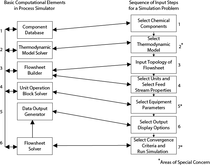
Figure 13.1 Relationship between Basic Computational Elements and Required Input to Solve a Process Simulation Problem
Component Database: This contains the parameters required to calculate the physical properties from the thermodynamic models.
Thermodynamic Model Solver: A variety of options for vapor-liquid (VLE) and liquid-liquid (LLE) equilibrium, enthalpy calculations, and other thermodynamic property estimations are available.
Flowsheet Builder: This part of the simulator keeps track of the flow of streams and equipment in the process being simulated. This information is input and displayed graphically.
Unit Operation Block Solver: Computational blocks or modules are available that allow energy and material balances and some design calculations to be performed for a wide variety of process equipment.
Data Output Generator: This part of the program serves to customize the results of the simulation in terms of an output report. Often, graphical displays of tower profiles, heating curves, and a variety of other useful process data can be produced.
Flowsheet Solver: This portion of the simulator controls the sequence of the calculations and the overall convergence of the simulation.
There are several other elements commonly found in process simulators that are not shown in Figure 13.1. For example, there are file control options, the option to use different engineering units, possibly some additional features associated with regressing data for thermodynamic models, and so on. The availability of these other options is dependent on the simulator used and will not be discussed further.
Also shown on the right-hand side of the diagram in Figure 13.1 are the seven general steps to setting up a process simulation problem. The general sequence of events that a user should follow in order to set up a problem on a simulator is as follows:
Select all of the chemical components that are required in the process from the component database.
Select the thermodynamic models required for the simulation. These may be different for different pieces of equipment. For example, to simulate a liquid-liquid extractor correctly, it is necessary to use a thermodynamic model that can predict liquid-phase activity coefficients and the existence of two liquid phases. However, for a pump in the same process, a less sophisticated model could be used.
Select the topology of the flowsheet to be simulated by specifying the input and output streams for each piece of equipment.
Select the properties (temperature, pressure, flowrate, vapor fraction, and composition) of the feed streams to the process.
Select the equipment specifications (parameters) for each piece of equipment in the process.
Select the way in which the results are to be displayed.
Select the convergence method and run the simulation.
Step 3 is achieved by constructing the flowsheet using equipment icons and connecting the icons with process streams. Sometimes, it is convenient to carry out this step first.
The interaction between the elements and steps and the general flow of information is shown by the lines on the diagram. Of the seven input steps given above, Steps 2, 5, and 7 are the cause of most problems associated with running process simulations. These areas will be covered in more detail in the following sections. However, before these topics are covered, it is worth looking at the basic solution algorithms used in process simulators.
There are basically three types of solution algorithms for process simulators [1]: sequential modular, equation solving (simultaneous nonmodular), and simultaneous modular.
In the sequential modular approach, the equations describing the performance of equipment units are grouped together and solved in modules—that is, the process is solved equipment piece by equipment piece. In the equation solving, or simultaneous nonmodular, technique, all the relationships for the process are written out together and then the resulting matrix of nonlinear simultaneous equations is solved to yield the solution. This technique is very efficient in terms of computation time but requires a lot of time to set up and is unwieldy. The final technique is the simultaneous modular approach, which combines the modularizing of the equations relating to specific equipment with the efficient solution algorithms for the simultaneous equation solving technique.
Of these three types, the sequential modular algorithm is by far the most widely used. In the sequential modular method, each piece of equipment is solved in sequence, starting with the first, followed by the second, and so on. It is assumed that all the input information required to solve each piece of equipment has been provided (see Section 13.2.5). Therefore, the output from a given piece of equipment, along with specific information on the equipment, becomes the input to the next piece of equipment in the process. Clearly, for a process without recycle streams, this method requires only one flowsheet iteration to produce a converged solution. The term flowsheet iteration means that each piece of equipment is solved only once. However, there may be many iterations for any one given piece of equipment, and batch units require time-series calculations to match the required scheduling of operations for the given unit. This concept is illustrated in Figure 13.2.

Figure 13.2 Solution Sequence Using Sequential Modular Simulator for a Process Containing No Recycles
The solution sequence for flowsheets containing recycle streams is more complicated, as shown in Figure 13.3. Figure 13.3(a) shows that the first equipment in the recycle loop (C) has an unknown feed stream (r). Thus, before Equipment C can be solved, some estimate of Stream r must be made. This leads to the concept of tear streams. A tear stream, as the name suggests, is a stream that is torn or broken. If the flowsheet in Figure 13.3(b) is considered, with the recycle stream torn, it can be seen, provided information is supplied about Stream r2, the input to Equipment C, that the flowsheet can be solved all the way around to Stream r1 using the sequential modular algorithm. Then Streams r1 and r2 are compared. If they agree within some specified tolerance, then there is a converged solution. If they do not agree, then Stream r2 is modified and the process simulation is repeated until convergence is obtained. The splitting or tearing of recycle streams allows the sequential modular technique to handle recycles. The convergence criterion and the method by which Stream r2 is modified can be varied, and multivariable successive substitution, Wegstein, and Newton-Raphson techniques [2, 3] are all commonly used for the recycle loop convergence. Usually, the simulator will identify the recycle loops and automatically pick streams to tear and a method of convergence. The tearing of streams and method of convergence can also be controlled by the user, but this is not recommended for the novice. Note that the implementation of heat integration (Chapter 15) may introduce (many) recycle streams.

Figure 13.3 The Use of Tear Streams to Solve Problems with Recycles Using the Sequential Modular Algorithm
13.2 Information Required to Complete a Process Simulation: Input Data
Referring back to Figure 13.1, each input block is considered separately. The input data for the blocks without asterisks (1, 3, 4, and 6) are quite straightforward and require little explanation. The remaining blocks (2, 5, and 7) are often the source of problems, and these are treated in more detail.
13.2.1 Selection of Chemical Components
Usually, the first step in setting up a simulation of a chemical process is to select which chemical components are going to be used. The simulator will have a databank of many components (more than a thousand chemical compounds are commonly included in these databanks). It is important to remember that all components—inerts, reactants, products, by-products, utilities, and waste chemicals—should be identified. If the chemicals that are needed are not available in the databank, then there are usually several ways that components (user-added components) can be added to the simulation. How to input data for user-added components is simulator specific, and the simulator user manual should be consulted.
13.2.2 Selection of Physical Property Models
Selecting the best physical property model is an extremely important part of any simulation. If the wrong property package or model is used, the simulated results will not be accurate and cannot be trusted. The choice of models is often overlooked by the novice, causing many simulation problems down the road. Simulators use both pure component and mixture properties. These range from molecular weight to activity-coefficient models. Transport properties (viscosity, thermal conductivity, diffusivity), thermodynamic properties (enthalpy, fugacity, K-factors, critical constants), and other properties (density, molecular weight, surface tension) are all important.
The physical property options are labeled as “thermo,” “method,” “property package,” or “databank” in common process simulators. There are pure-component and mixture sections, as well as a databank. For temperature-dependent properties, different functional forms are used (from extended Antoine equation to polynomial to hyperbolic trigonometric functions). The equation appears on the physical property screen or in the help utility.
For pure-component properties, the simulator has information in its databank for thousands of compounds. Some simulators offer a choice between DIPPR and proprietary databanks. These are largely the same, but the proprietary databank may contain additional components, petroleum cuts, electrolytes, and so on. DIPPR is the Design Institute for Physical Property Research (a part of AIChE), and sharing of process data across different simulators (e.g., Aspen Plus, CHEMCAD, Aspen HYSYS, PRO/II, SuperPro Designer) can be enhanced by using that databank. (Note that some proprietary databanks may not be supplied in the academic versions of these simulators.) All simulators also have built-in procedures to estimate pure-component properties from group-contribution and other techniques. The details of these techniques are covered in standard chemical engineering thermodynamics texts [4–6] and are not described here. However, the user must be aware of any such estimations made by the simulator. Any estimation, by definition, increases the uncertainty in the results of the simulation. The entry in the databank for each component should indicate estimations. For example, many long-chain hydrocarbons have no experimental critical point because they decompose at relatively low temperatures. However, because critical temperatures and pressures are needed for most thermodynamic models, they must be estimated. Although these estimations allow the use of equation-of-state and some other models, one must never assume that these are experimental data.
Heat capacities, densities, and critical constants are the most important pure-component data for simulation. The transport and other properties are used in equipment sizing calculations. The techniques used in the simulators are no more accurate than those covered in transport, thermodynamics, unit operations, and separations courses—they are just easier to apply.
Even though simple mass and energy balances cannot be done by the simulator without the above-mentioned, pure-component properties, often the most influential decision in a simulation is the choice of a model to predict phase equilibria. Several of the popular simulators have expert systems to help the user select the appropriate model for the system. The expert system determines the range (usually with additional user input) of operating temperatures and pressures covered by the simulation and, with data on the components to be used, makes an informed guess of the thermodynamic models that will be best for the process being simulated. The word expert should not be taken too seriously! The expert-system choice is only a first guess. Additionally, the model chosen may not be best for a given piece of equipment. A moderately complex simulation may use at least two different thermodynamic packages for different parts of the flowsheet.
Due to the importance of thermodynamic model selection and the many problems that the wrong selection leads to, a separate section (Section 13.4) is dedicated to this subject. An example of how the wrong thermodynamic package can cause serious errors is given in Example 13.1.
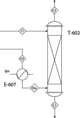
Consider the HCl absorber (T-602) in the separation section of the allyl chloride process, Figure C.3 in Appendix C. This equipment is shown in Figure E13.1. The function of the absorber is to contact countercurrently Stream 10a, containing mainly propylene and hydrogen chloride, with water, Stream 11. The HCl is highly soluble in water and is almost completely absorbed to form 32 wt% hydrochloric acid, Stream 12. The gas leaving the top of the absorber, Stream 13, is almost pure propylene, which is cleaned and then recycled.
Solution
Table E13.1 shows the results for the two outlet streams from the absorber—Streams 12 and 13—for two simulations, each using a different thermodynamic model for the vapor-liquid equilibrium calculations. The second and third columns in the table show the results using the SRK (Soave [7], Redlich and Kwong [8]) model, which is the preferred model for many common organic components. The fourth and fifth columns show the results using a model that is specially designed to deal with ionic type compounds (HCl) that dissolve in water and then dissociate. The difference in results is remarkable. The HCl-water system is highly nonideal, and, even though the absorption of an acid gas into aqueous solutions is quite common, the SRK model is not capable of correctly modeling the phase behavior of this system. With the SRK model, virtually all the HCl leaves the absorber as a gas. Clearly, if the simulation were done using only the SRK model, the results would be drastically in error. This result is especially disturbing because SRK is the default thermodynamics package in many simulators.
Table E13.1 Results of Simulation of HCl Absorption Using Two Different Physical Property Models
Using SRK Model |
Using PPAQ* Model |
|||
Phase Component Flows (kmol/h) |
Stream 12 Liquid |
Stream 13 Vapor |
Stream 12 Liquid |
Stream 13 Vapor |
Propylene |
0.05 |
57.48 |
— |
57.53 |
Allyl chloride |
0.01 |
— |
0.01 |
— |
Hydrogen chloride |
0.91 |
18.78 |
19.11 |
0.58 |
Water |
81.37 |
0.63 |
81.88 |
0.12 |
Total |
82.34 |
76.89 |
101.00 |
58.23 |
* This is a model used in the CHEMCAD simulator especially for HCl-water and similar systems. |
||||
More details of model selection are given in Section 13.4.
The importance of thermodynamic model selection and its impact on the validity of the results of a simulation are discussed at length by Horwitz and Nocera [9], who warn
“You absolutely must have confidence in the thermodynamics that you have chosen to represent your chemicals and unit operations. This is your responsibility, not that of the software simulation package. If you relinquish your responsibility to the simulation package, be prepared for dire consequences.”
13.2.3 Selection and Input of Flowsheet Topology
The most reliable way to input the topology of the process flow diagram is to make a sketch on paper and have this in front of you when you construct the flowsheet on the simulator. Contrary to the rules given in Chapter 1 on the construction of PFDs, every time a stream splits or several streams combine, a simulator equipment module (splitter or mixer) must be included. These “phantom” units were introduced in Chapter 5 and are useful in tracing streams in a PFD as well as being required for the simulator. They are required in the simulator so it “knows” to do the necessary material and energy balances on mixers and splitters; however, they should not appear on a PFD. Certain conventions in the numbering of equipment and streams are used by the simulator to keep track of the topology and connectivity of the streams. When using the graphical interface, the streams and equipment are usually numbered sequentially in the order they are added. These can be altered by the user if required. Care must be taken when connecting batch and continuous unit operations, because it is often assumed that “continuous” units approach steady state instantaneously.
13.2.4 Selection of Feed Stream Properties
As discussed in Section 13.1, the sequential modular approach to simulation requires that all feed streams be specified (composition, flowrate, vapor fraction, temperature, and pressure). In addition, estimates of recycle streams should also be made. Although feed properties are usually well defined, some confusion may exist regarding the number and type of variables that must be specified to define the feed stream completely. In general, feed streams will contain n components and consist of one or two phases. For such feeds, a total of n + 2 specifications completely defines the stream. This is a consequence of the phase rule. Providing the flowrate (kmol/h, kg/s, etc.) of each component in the feed stream takes care of n of these specifications. The remaining two specifications should also be independent. For example, if the stream is one phase, then giving the temperature and pressure of the stream completely defines the feed. Temperature and pressure also completely define a multicomponent stream having two phases. However, if the feed is a single component and contains two phases, then temperature and pressure are not independent. In this case, the vapor fraction and either the temperature or the pressure must be specified. Vapor fraction can also be used to specify a two-phase multicomponent system, but if used, only temperature or pressure can be used to specify the feed completely. To avoid confusion, it is recommended that vapor fraction (vf) be specified only for saturated vapor (vf = 1), saturated liquid (vf = 0), and two-phase, single-component (0 < vf < 1) streams. All other streams should be specified using the temperature and pressure.
Use the vapor fraction (vf) to define feed streams only for saturated vapor (vf = 1), saturated liquid (vf = 0), and two-phase, single-component (0 < vf < 1) streams.
By giving the temperature, pressure, and vapor fraction for a feed, the stream is overspecified and errors will result.
13.2.5 Selection of Equipment Parameters
It is worth pointing out that process simulators, with a few exceptions, are structured to solve process material and energy balances, reaction kinetics, reaction equilibrium relationships, phase-equilibrium relationships, and equipment performance relationships for equipment in which sufficient process design variables and batch operations scheduling have been specified. For example, consider the design of a liquid-liquid extractor to remove 98% of a component in a feed stream using a given solvent. In general, a process simulator will not be able to solve this design problem directly; that is, it cannot determine the number of equilibrium stages required for this separation. However, if the problem is made into a simulation problem, then it can be solved by a trial-and-error technique. Thus, by specifying the number of stages in the extractor, case studies in which the number of stages are varied can be performed, and this information can be used to determine the correct number of stages required to obtain the desired recovery of 98%. In other cases, such as a plug flow reactor module, the simulator can solve the design problem directly—that is, calculate the amount of catalyst required to carry out the desired reaction. Therefore, before starting a process simulation, it is important to know what equipment parameters must be specified in order for the process to be simulated.
There are essentially two levels at which a process simulation can be carried out. The first level, Level 1, is one in which the minimum data are supplied in order for the material and energy balances to be obtained. The second level, Level 2, is one in which the simulator is used to do as many of the design calculations as possible. The second level requires more input data than the first. An example of the differences between the two levels is illustrated in Figure 13.4, which shows a heat exchanger in which a process stream is being cooled using cooling water. At the first level, Figure 13.4(a), the only information that is specified is the desired outlet condition of the process stream—for example, pressure and temperature or vapor fraction—if the stream is to leave the exchanger as a two-phase mixture. However, this is enough information for the simulator to calculate the duty of the exchanger and the properties of the process stream leaving the equipment. At the second level, Figure 13.4(b), additional data are provided: the inlet and desired outlet temperature for the utility stream, the fact that the utility stream is water, the overall heat transfer coefficient, and the heat-exchanger configuration or log-mean-temperature-correction factor, F. Using this information, the simulator calculates the heat-exchanger duty, the required cooling water flowrate, and the required heat transfer area.
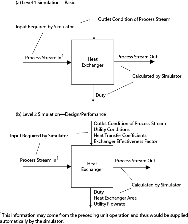
When attempting to do a simulation on a process for the first time, it is recommended that the minimum data required be provided for a Level 1 simulation. When a satisfactory, converged solution is obtained, more data can be provided to obtain desired design parameters, that is, a Level 2 solution.
When first simulating a process, input only the data required to perform the material and energy balances for the process.
The structure of the process simulator will determine the exact requirements for the input data, and such information will be available in the user manual for the software or on help screens. However, for Level 1 simulations, a brief list of typical information is presented below that may help a novice user prepare the input data for a process simulation.
Pumps, Compressors, and Power Recovery Turbines (Expanders). For pumps, the desired pressure of the fluid leaving the pump or the desired pressure increase of the fluid as it flows through the pump and the efficiency are all that is required.
For compressors and turbines, the desired pressure of the fluid leaving the device or the desired pressure increase of the fluid as it flows through the equipment is required. In addition, the efficiency and the mode of compression or expansion—adiabatic, isothermal, or polytropic—are required.
Heat Exchangers. For exchangers with a single process stream exchanging energy with a utility stream, all that is required is the condition of the exit process stream. This can be the exit pressure (or pressure drop) and temperature (single-phase exit condition) or the exit pressure and vapor fraction (two-phase exit condition).
For exchangers with two or more process streams exchanging energy (as might be the case when heat integration is being considered), the exit conditions (pressure and temperature or vapor fraction) for both streams are required. However, the system should not be overspecified. Of the two flowrates and four temperatures (two input, two output), one should not be specified, and the simulator will calculate the unknown variable from the energy balance. The user must be aware of the possibility of temperature crosses in heat-exchange equipment. The simulator may or may not warn the user that a temperature cross has occurred but will continue to simulate the rest of the process. The results from such a simulation will not be valid, and the temperature cross must be remedied before a correct solution can be obtained. Therefore, it is recommended that the user check the temperature profiles for all heat exchangers after the simulation.
Fired Heaters (Furnaces). The same requirements for heat exchangers with a single process fluid apply to fired heaters.
Mixers and Splitters. Mixers and splitters used in process simulators are usually no more than simple tees in pipes. Unless special units must be provided—for example, when the fluids to be mixed are very viscous and in-line mixers might be used—the capital investment of these units can be assumed to be zero.
Mixers represent points where two or more process streams come together. The only required information is an outlet pressure or pressure drop at the mixing point. Usually, the pressure drop associated with the mixing of streams is small, and the pressure drop can be assumed to be equal to zero with little error. If feed streams enter the mixer at different pressures, the simulator assignes the outlet stream pressure to be at the lowest pressure of the mixing streams. This assumption causes little error in the material and energy balance. However, since the pressures of mixing streams will be equal, if a system is actually designed with streams mixing at different pressures, the pressures will equalize by adjusting the flowrates, and the process will not operate as designed. It is recommended that valves be added to the simulation so that mixing streams are at the same pressure.
Splitters represent points at which a process stream splits into two or more streams with different flowrates but identical compositions. The required information is the outlet pressure or pressure drop across the device and the relative flows of the output streams. Usually, there is little pressure drop across a splitter, and all streams leaving the unit are at the same pressure as the single feed stream. In a batch operation, the splitter can be assigned on and off times to divert the inlet flow to various other units on a schedule.
Valves. Either the outlet pressure or pressure drop is required.
Reactors. The way in which reactors are specified depends on a combination of the input information required and the reactor category. Generally there are four categories of reactor: stoichiometric reactor, kinetic (plug flow or CSTR) reactor, equilibrium reactor, and batch reactor. All these reactor configurations require input concerning the thermal mode of operation: adiabatic, isothermal, amount of heat removed or added. Additional information is also required. Each reactor type is considered separately below.
Stoichiometric Reactor: This is the simplest reactor type that can be simulated. The required input data are the number and stoichiometry of the reactions, the temperature and pressure, and the conversion of the limiting reactant. Reactor configuration (plug flow, CSTR) is not required because no estimate of reactor volume is made. Only basic material and energy balances are performed.
Kinetic (Plug Flow and CSTR) Reactor: This reactor type is used to simulate reactions for which kinetics expressions are known. The number and stoichiometry of the reactions are required input data. Kinetics constants (Arrhenius rate constants and Langmuir-Hinshelwood constants, if used) and the form of the rate equation (simple first-order, second-order, Langmuir-Hinshelwood kinetics, etc.) are also required. Reactor configuration (plug flow, CSTR) is required. Options may be available to simulate cooling or heating of reactants in shell-and-tube reactor configurations in order to generate temperature profiles in the reactor. If the reactor volume (or shell-and-tube configuration details) is provided, the simulator determines the outlet conditions. Some simulators allow the fractional conversion of a reactant to be specified and calculate the necessary volume.
Equilibrium Reactor: As the name implies, this reactor type is used to simulate reactions that obtain or approach equilibrium conversion. The number and stoichiometry of the reactions and the fractional approach to equilibrium are the required input data. In addition, equilibrium constants as a function of temperature may be required for each reaction or may be calculated directly from information in the database. In this mode, the user has control over which reactions should be considered in the analysis.
Minimum Gibbs Free Energy Reactor: This is another common form of the equilibrium reactor. In the Gibbs reactor, the outlet stream composition is calculated by a free energy minimization technique. Usually data are available from the simulator’s databank to do these calculations. The only input data required are the list of components that one anticipates in the output from the reactor. In this mode the equilibrium conversion that would occur for an infinite residence time is calculated.
Batch Reactor: This reactor type is similar to the kinetic reactor (and requires the same kinetics input), except that it is batch. The volume of the reactor is specified. The feeds, product compositions, and reactor temperature (or heat duty) are scheduled (i.e., they are specified as time series).
As a general rule, the least complicated reactor module that will allow the heat and material balance to be established should be used. The reactor module can always be substituted later with a more sophisticated one that allows the desired design calculations to be performed. It should also be noted that a common error made in setting up a reactor module is the use of the wrong component as the limiting reactant when a desired conversion is specified. This is especially true when several simultaneous reactions occur, and the limiting component may not be obvious solely from the amounts of components in the feed.
Flash Units. In simulators, the term flash refers to the module that performs a single-stage vapor-liquid equilibrium calculation. Material, energy, and phase-equilibrium equations are solved for a variety of input parameter specifications. In order to specify completely the condition of the two output streams (liquid and vapor), two parameters must be input. Many combinations are possible—for example, temperature and pressure, temperature and heat load, or pressure and mole ratio of vapor to liquid in exit streams. Often, the flash module is a combination of two pieces of physical equipment, that is, a a heat exchanger followed by a phase separator. These should appear as separate equipment on the PFD. Note that a flash unit can also be specified for batch operation, in which case the unit can serve as a surge or storage vessel.
Distillation Columns. Usually, both rigorous methods (stage-by-stage calculations) and shortcut methods (like Fenske, Underwood, and Gilliland relationships using key components) are available. In preliminary simulations, it is advisable to use shortcut methods. The advantage of the shortcut methods is that they allow a design calculation (which estimates the number of theoretical plates required for the separation) to be performed. For preliminary design calculations, this is a very useful option and can be used as a starting point for using the more rigorous algorithms, which require that the number of theoretical stages be specified. It should be noted that, in both methods, the calculations for the duties of the reboiler and condenser are carried out in the column modules and are presented in the output for the column. Detailed design of these heat exchangers (area calculations) often cannot be carried out during the column simulation.
Shortcut Module: The required input for the design mode consists of identification of the key components to be separated, specification of the fractional recoveries of each key component in the overhead product, the column pressure and pressure drop, and the ratio of actual to minimum reflux ratio to be used in the column. The simulator will estimate the number of theoretical stages required, the exit stream conditions (bottom and overhead products), optimum feed location, and the reboiler and condenser duties.
If the shortcut method is used in the rating (or performance) mode, the number of equilibrium stages must also be specified, but the R/Rmin is calculated.
Rigorous Module: The number of theoretical stages must be specified, along with the condenser and reboiler type (total or partial), column pressure and pressure drop, feed tray locations, and side product locations (if side stream products are desired). Even though total condensers and total reboilers are not equilibrium stages, they are included in the stage count in a rigorous distillation module, so the simulator can do the required calculations for them. That is why the type of condenser and reboiler must be specified, so the simulator “knows” whether to do an equilibrium calculation or whether to take saturated vapor to saturated liquid (or vice versa). In addition, the total number of specifications given must be equal to the number of products (top, bottom, and side streams) produced. These product specifications are often a source of problems, and this is illustrated in Example 13.2.
Several rigorous modules may be available in a given simulator. Differences between the modules are the different solution algorithms used and the size and complexity of the problems that can be handled. Stage-to-stage calculations can be handled for several hundred stages in most simulators. In addition, these modules can be used to simulate accurately other equilibrium-staged devices, for example, absorbers and strippers.
Batch Distillation: This module is similar to the rigorous module, except that feeds and product draws are on a schedule (not continuous). Therefore, the start and stop times of the feeds and products must be specified, and a time series of tray concentrations and temperatures is generated by the simulator.
Consider the benzene recovery column in the toluene hydrodealkylation process shown in Figure 1.5. This column is redrawn in Figure E13.2. The purpose of the column is to separate the benzene product from unreacted toluene, which is recycled to the front end of the process. The desired purity of the benzene product is 99.6 mol%. The feed and the top and bottoms product streams are presented in Table E13.2, which is taken from Table 1.5.

Figure E13.2 Benzene Column in Toluene Hydrodealkylation Process (from Figure 1.5)
Table E13.2 Stream Table for Figure E13.2
Component |
Stream 10 |
Stream 15 |
Stream 19 |
Stream 11 |
Hydrogen |
0.02 |
— |
0.02 |
— |
Methane |
0.88 |
— |
0.88 |
— |
Benzene |
106.3 |
105.2 |
— |
1.1 |
Toluene |
35.0 |
0.4 |
— |
34.6 |
Solution
There are many ways to specify the parameters needed by the rigorous column algorithm used to simulate this tower.
Two examples are given:
The key components for the main separation are identified as benzene and toluene. The composition of the top product is specified to be 99.6 mol% benzene, and the recovery (not the mole fraction) of toluene in the bottoms product is 0.98.
The top composition is specified to be 99.6 mol% benzene, and the recovery of benzene in the bottoms product is 0.01.
The first specification violates the material balance, whereas the second specification does not. Looking at the first specification, if 98% of the toluene in the feed is recovered in the bottoms product, then 2% or 0.7 kmol/h must leave with the top product. Even if the recovery of benzene in the top product were 100%, this would yield a top composition of 106.3 kmol/h benzene and 0.7 kmol/h toluene. This corresponds to a mole fraction of 0.993. Therefore, the desired mole fraction of 0.996 can never be reached. Thus, by specifying the recovery of toluene in the bottoms product, the specification for the benzene purity is automatically violated.
The second specification shows that both specifications can be achieved without violating the material balance. The top product contains 99% of the feed benzene (105.2 kmol/h) and 0.4 kmol/h toluene, which gives a top composition of 99.6 mol% benzene. The bottoms product contains 1.0% of the feed benzene (1.1 kmol/h) and 34.6 kmol/h of toluene.
When giving the top and bottom specifications for a distillation column, make sure that the specifications do not violate the material balance.
If problems continue to exist, one way to ensure that the simulation will run is to specify the top reflux rate and the boil-up rate (reboiler duty). Although this strategy will not guarantee the desired purities, it will allow a base case to be established. With subsequent manipulation of the reflux and boil-up rates, the desired purities can be obtained. Another strategy that may be useful when a high purity is needed is to start with a lower purity and then increase the purity specification in steps to the desired purity. This only works if the simulation is not “reset” after each run, that is, the previous result is used as the starting point each time.
Absorbers and Strippers. Usually these units are simulated using the rigorous distillation module given above. The input streams and the number of equilibrium stages are specified, and the outlet streams are obtained. The main difference in simulating this type of equipment is that condensers and reboilers are not normally used. In addition, there are two feeds to the unit: one feed enters at the top and the other at the bottom. It may also be necessary to toggle a setting to indicate that an absorber/stripper is being simulated.
Liquid-Liquid Extractors. A rigorous tray-by-tray module is used to simulate this multistaged equipment. The input streams and the number of equilibrium stages are specified, and the outlet streams are obtained. It is imperative that the thermodynamic model for this unit be capable of predicting the presence of two liquid phases, each with appropriate liquid-phase activity coefficients. This module is usually different from the module that simulates vapor-liquid systems, like distillation, absorption, and stripping.
13.2.6 Selection of Output Display Options
Several options will be available to display the results of a simulation. Often, a report file can be generated and customized to include a wide variety of stream and equipment information. In addition, a simulation flowsheet (not a PFD); T-Q diagrams for heat exchangers; vapor and liquid flows; temperature and composition profiles (tray-by-tray) for multistaged equipment; temperature and composition profiles along a tubular reactor; scheduling charts for batch operations; environmental parameters for exit streams; and a wide variety of phase diagrams for streams can be generated. The user manual should be consulted for the specific options available for the simulator you use.
13.2.7 Selection of Convergence Criteria and Running a Simulation
For equipment requiring iterative solutions, there will be user-selectable convergence and tolerance criteria in the equipment module. There will also be convergence criteria for the whole flowsheet simulation, which can be adjusted by the user.
The two most important criteria are number of iterations and tolerance. These criteria will often have default values set in the simulator. These default values should be used in initial simulations. If problems arise, these values should be adjusted, but it may also be necessary to choose a different convergence method.
If the simulation has not converged, the results do not represent a valid solution and should not be used.
When convergence is not achieved, three common causes are as follows:
The problem has been ill posed. This normally means that an equipment specification has been given incorrectly. For example, see the first specification in Example 13.2 for the rigorous column module.
The tolerance for the solution has been set too tightly, and convergence cannot be obtained to the desired accuracy no matter how many solution iterations are performed.
The number of iterations is not sufficient for convergence. This occurs most often when the flowsheet has many recycle streams. Rerunning the flowsheet simulation with the results from the preceding run may give a converged solution. If convergence is still not obtained, then one way to address this problem is to remove as many recycle streams as possible. The simulation is then run, and the recycle streams are added back, one by one, using the results from the preceding simulation as the starting point for the new one. This method is discussed in more detail in Section 13.3.
Of the three reasons, the first one is by far the most common.
The most common reason for the failure of a simulation to converge is the use of incorrect or impossible equipment specifications.
13.2.8 Common Errors in Using Simulators
As mentioned previously, simulators perform some calculations that are not physically correct, and some unit operations in simulators do not correspond to acutal equipment. Two examples were previously mentioned. One is that mixing streams will be at the same pressure, not the lower of the pressures of the mixing streams, which is what simulators assume. It is the user’s responsibility to add valves to the higher-pressure streams so that mixing streams are at the same pressure. Another example is the “flash” tank that operates at a different temperature from the feed stream without a heat exchanger. In reality, the “flash” operation is a partial vaporization or partial condensation, which requires a heat exchanger. The correct equipment configuration is a heat exchanger followed by a tank to disengage the vapor and liquid phases. The tank can be modeled in a simulator as a flash operating at the same conditions as the feed stream, which is the exit stream from the heat exchanger. It is also important to make use of the information available within a simulator, for example, temperature and composition profiles in tubular reactors and T-xy diagrams for heat exchangers.
Table 13.1 summarizes some common errors made by students when using process simulators.
Table 13.1 Commonly Observed Simulation Errors
Physical Situation |
Error Observed |
Correct Method |
Incorrect use of flash unit simulation |
Including flash unit with heat load, so temperature changes “magically” |
Simulate as heat exchanger followed by flash unit operating at inlet conditions |
Mixing points |
Mixing streams at different pressures, outlet stream at lowest pressure (simulator default) |
Add valves to input streams to mixer as appropriate to ensure mixing streams at same pressure |
Zoned analysis required |
For phase change operations, only one zone used with one heat transfer coefficient |
Simulate each zone as separate heat exchanger with separate heat transfer coefficient, but PFD shows one heat exchanger (some simulators allow zoned analysis in heat exchange unit if each zone’s heat transfer coefficient is provided) |
LMTD correction factor required but ignored |
Standard configuration in industry is 1-2 exchanger |
Check approach temperatures to see if more shell passes are needed, often occurs if heat integration used |
Inappropriate reactor size |
Desired product rate approaches constant value or starts to decrease |
Examine reactor profiles to determine if reactor is oversized or if selectivity is decreasing |
Real vs. actual trays |
Column design and cost calculated for number of equilibrium trays |
Include tray efficiency in simulation or add trays when performing cost calculation |
Column pressure drop |
Column assumed to be at constant pressure or pressure drop chosen does not correspond to reality |
Include pressure drop and make sure pressure drop per tray roughly corresponds to weir height, and that weir height is not too small or not more than 50% of tray spacing; or assume weir height (typically 4-6 in and less than half of tray spacing) and include pressure drop in simulation |
13.3 Handling Recycle Streams
Recycle streams are very important and common in process flowsheets. Computationally, they can be difficult to handle and are often the cause for unconverged flowsheet simulations. There are ways in which the problems caused by recycle streams can be minimized. When a flowsheet is simulated for the first time, it is wise to consider carefully any simplifications that may help the convergence of the simulation. Consider the simulation of the DME flowsheet illustrated in Figure B.1.1, Appendix B. This flowsheet is shown schematically in Figure 13.5(a). The DME process is simple, no by-products are formed, the separations are relatively easy, and the methanol can be purified easily prior to being recycled to the front end of the process. In attempting to simulate this process for the first time, it is evident that two recycle streams are present. The first is the unreacted methanol that is recycled to the front of the process, upstream of the reactor. The second recycle loop is due to the heat integration scheme used to preheat the reactor feed using the reactor effluent stream. The best way to simulate this flowsheet is to eliminate the recycle streams as shown in Figure 13.5(b). In this figure, two separate heat exchangers have been substituted for the heat integration scheme. These exchangers allow the streams to achieve the same changes in temperature while eliminating the interaction between the two streams. The methanol recycle is eliminated in Figure 13.5(b) by producing a methanol pseudo-output stream. The simulation of the flowsheet given in Figure 13.5(b) is straightforward; it contains no recycle streams and will converge in a single flowsheet iteration. Troubleshooting of the simulation, if input errors are present, is very easy because the flowsheet converges very quickly. Once a converged solution has been obtained, the recycle streams can be added back. For example, the methanol recycle stream would be introduced back into the simulation. The composition of this stream is known from the preceding simulation, and this will be a very good estimate for the recycle stream composition. The simulation is then run with the preceding simulation as the starting point. Once the simulation has been run successfully with the methanol recycle stream, the heat integration around the reactor can be added back and the simulation run again. Although this method may seem unwieldy, it does provide a reliable method for obtaining a converged simulation.
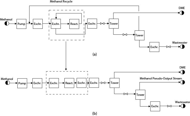
Figure 13.5 Block Flow Diagram for DME Process Showing (a) Recycle Structure and (b) Elimination of Recycles
For the DME flowsheet in Figure 13.5, the unreacted methanol that was recycled was almost pure feed material. This means that the estimate of the recycle stream composition, obtained from the once-through simulation using Figure 13.5(b), was very good. When the recycle stream contains significant amounts of by-products, as is the case with the hydrogen recycle stream in Figure 1.5 (Streams 5 and 7), the estimate of the composition using a once-through simulation will be significantly different from the actual recycle stream composition. For such cases, when purification of the recycle stream does not occur, it is best to keep this recycle stream in the flowsheet and eliminate all other recycle streams for the first simulation. Once a converged solution is reached, the other recycle streams can be added back one at a time.
Often, a series of case studies will need to be run using a base-case simulation as a starting point. This is especially true when performing a parametric optimization on the process (see Chapter 14). When performing such case studies, it is wise to make small changes in input parameters in order to obtain a converged simulation. For example, assume that a converged simulation for a reactor module at 350°C has been obtained, and a case study needs to be run at 400°C. When the equipment temperature in the reactor module is changed and the simulation is rerun, it may be found that the simulation does not converge. If this is the case, then, for example, start with the base-case run, change the reactor temperature by 25°C, and see whether it converges. If it does, then the input can be changed by another 25°C to give the desired conditions, and so on. The use of small increments or steps when simulating changes in flowsheets often produces a converged simulation when a single large change in input will not.
Often when simulating a process, it is the flowrate of products (not feeds) that is known—for example, production of 60,000 tonne/y of chemical X, with a purity of 99.9 wt%. If a converged solution has been found in which all the product specifications have been met except that the flowrate of primary product is not at the desired value, it is a simple matter to multiply all the feeds to the process by a factor to obtain the desired flowrate of the product; that is, the solution is scaled up or down by a constant factor and the simulation rerun to get the correct equipment specifications.
For more advanced simulation applications, such as optimizing or simulating existing plants, it may be necessary or useful to use controller modules (also called design specifications, depending on the simulator) in the simulation to obtain a desired result. For example, in a recycle loop, it might be required that the ratio of two components entering a reactor be set at some fixed value. A controller module could be used to adjust the purge flowrate from the recycle stream to obtain this ratio. A controller module can also be used to specify the feed necessary for the product flowrate to be at a specific value. The use of controller modules introduces additional recycle loops. The way in which specifications for controllers are given can cause additional convergence problems, and this topic is covered in detail by Schad [10].
13.4 Choosing Thermodynamic Models
The results of any process simulation are never better than the input data, especially the thermodynamic data.
Everything from the energy balance to the volumetric flowrates to the separation in the equilibrium-stage units depends on accurate thermodynamic data.
If reaction kinetics information is missing, the simulator cannot calculate the conversion from a given reactor volume. Because such a calculation is not possible, only equilibrium reactor modules and those with specified conversions can be used.
Only a few, readily available data are required to estimate the parameters in simple thermodynamic models. If the critical temperature and critical pressure are known for each pure component, the parameters for simple, cubic equations of state can be estimated. Even if these critical properties are unknown, they in turn can be estimated from one vapor pressure and one liquid density. Group-contribution models require even less information: merely the chemical structure of the molecule. However, these estimations can never be as accurate as experimental data. In thermodynamics, as elsewhere, you get only what you pay for—or less!
Using the default thermodynamics packages in a process simulator will often lead to an erroneous solution.
Compounding this problem is the development and implementation of expert systems to help choose the thermodynamic model. These methods are a good starting point but verification through comparison with real data is always necessary.
A safe choice of thermodynamic model requires knowledge of the system, the calculation options of the simulator, and the margin of error. In this section, guidance on choosing and using a thermodynamic model is given. In an academic setting, the choice of thermodynamic model affects the answers but not the ability of the student to learn how to use a process simulator—a key aspect of this book. Therefore, the examples throughout this book use simplistic thermodynamic models to allow easy simulation. In any real problem, where the simulation will be used to design or troubleshoot a process, the proper choice of thermodynamic model is essential. This section focuses on the key issues in making that choice, in using experimental data, and in determining when additional data are needed.
It has been assumed that the reader understands the basics of chemical engineering thermodynamics as covered in standard textbooks [4–6]. As pointed out before, it is extremely important that the chemical engineer performing a process simulation understand the thermodynamics being used. In a course, the instructor can often provide guidance. The help facility of the process simulator provides a refresher on details of the model choices; however, these descriptions do not include the thermodynamics foundation required for complete understanding. If the descriptions in the help facility are more than a refresher, the standard thermodynamics textbooks should be consulted.
If the thermodynamic option used by the process simulator is a mystery, the meaning of the results obtained from the simulation will be equally mysterious.
13.4.1 Pure-Component Properties
Physical properties such as density, viscosity, thermal conductivity, and heat capacity are generally not difficult to predict accurately in a simulation. The group-contribution methods are reasonably good, and simulator databanks include experimental data for more than a thousand substances. Although these correlations have random and systematic errors of several percent, this is close enough for most purposes. (However, they are not sufficient when paying for a fluid crossing a boundary based on volumetric flowrate.) As noted in Section 13.2.2, it is important always to be aware of which properties are estimated and which are from experimental measurements.
13.4.2 Enthalpy
Although the pure-component heat capacities are calculated with acceptable accuracy, the enthalpies of phase changes often are not. Care should be taken in choosing the enthalpy model for a simulation. If the enthalpy of vaporization is an important part of a calculation, simple equations of state should be used with caution. In fact, the “latent heat” or “ideal” options often give more accurate results. If the substance is above or near its critical temperature, equations of state must be used, but the user must beware, especially if polar substances such as water are present.
13.4.3 Phase Equilibria
Extreme care must be exercised in choosing a model for phase equilibria (sometimes called the fugacity coefficient, K-factor, or fluid model). Whenever possible, phase-equilibrium data for the system should be used to regress the parameters in the model, and the deviation between the model predictions and the experimental data should be studied.
There are two general types of fugacity models: equations of state and liquid-state activity-coefficient models. An equation of state is an algebraic equation for the pressure of a mixture as a function of the composition, volume, and temperature. Through standard thermodynamic relationships, the fugacity, enthalpy, and so on for the mixture can be determined. These properties can be calculated for any density; therefore, both liquid and vapor properties, as well as supercritical phenomena, can be determined.
Activity-coefficient models, however, can only be used to calculate liquid-state fugacities and enthalpies of mixing. These models provide algebraic equations for the activity coefficient (γi) as a function of composition and temperature. Because the activity coefficient is merely a correction factor for the ideal-solution model (essentially Raoult’s Law), it cannot be used for supercritical or “noncondensable” components. (Modifications of these models for these types of systems have been developed, but they are not recommended for the process simulator user without consultation with a thermodynamics expert.)
Equations of state are recommended for simple systems (nonpolar, small molecules) and in regions (especially supercritical conditions for any component in a mixture) where activity-coefficient models are inappropriate. For complex liquid mixtures, activity-coefficient models are preferred, but only if all of the binary interaction parameters (BIPs) are available.
Equations of State. The default fugacity model is often either the SRK (Soave-Redlich-Kwong) or the PR (Peng-Robinson) equation. They (like most popular equations of state) normally use three pure-component parameters per substance and one binary-interaction parameter per binary pair. Although they give qualitatively correct results even in the supercritical region, they are known to be poor predictors of enthalpy changes, and (except for light hydrocarbons) they are not quantitatively accurate for phase equilibria.
The predicted phase equilibrium is a strong function of the binary interaction parameters (BIPs). Process simulators have regression options to determine these parameters from experimental phase-equilibrium data. The fit gives a first-order approximation for the accuracy of the equation of state. This information should always be considered in estimating the accuracy of the simulation. Additional simulations should be run with perturbed model parameters to get a feel for the uncertainty, and the user should realize that even this approach gives an optimistic approximation of the error introduced by the model. If BIPs are provided in the simulator and the user has no evidence that one equation of state is better than another, then a separate, complete simulation should be performed for each of these equations of state. The difference between the simulations is a crude measure of the uncertainty introduced into the simulation by the uncertainty in the models. Again, the inferred uncertainty will be on the low side.
Monte-Carlo simulations (see Section 10.7) can be done with the results of the regression; however, process simulators are not currently equipped to perform these directly. A simpler approach is to perform the simulation with a few different values of the BIPs for the equation of state. These values are typically 0.01 to 0.10. Larger values are rare, except in highly asymmetric systems. However, the difference between results calculated with values of, say, 0.01 and 0.02 can be large.
If BIPs are available for only a subset of the binary pairs, caution should be exercised. Assuming the unknown BIPs to be zero can be dangerous. Group-contribution models for estimating BIPs for equations of state can be used with caution.
There may be dozens of equation-of-state options, including different modifications of the same equation of state, plus a few mixing-rule choices. For polar or associating components or for heavy petroleum cuts, the help facility of the simulator should be consulted. Because different choices are available on the different simulators, they will not be covered here.
For most systems containing hydrocarbons and light gases, an equation of state is the best choice. Peng-Robinson or Soave-Redlich-Kwong are good initial choices. (Note that neither the van der Waals nor Redlich-Kwong equation is a standard choice in simulators. These two equations of state were tremendous breakthroughs in fluid property models, but they were long ago supplanted by other models that give better quantitative results.) VLE (vapor-liquid equilibrium) data for each binary system can then be used with the regression utility to calculate the BIPs for the binary pairs and to plot the resulting model predictions against the experimental data. This regression is done separately for each equation of state. The equation that gives a better fit in the (PTxy) region of operation of the unit operation of interest is then used. If phase-equilibrium data are available at different temperatures, the temperature-dependent BIP feature of the simulator can be used. In the simulator databank, many BIPs are already regressed and available.
If neither simple equation of state adequately reproduces the experimental data, one of the other equations of state or other mixing rules, or a temperature-dependent BIP, may be needed. These often work better for polar-nonpolar systems. However, running the simulation more than once with different BIPs and with different thermodynamic models to judge the uncertainty of the result is recommended, as shown in Example 13.3. If the difference between the simulations seriously affects the viability of the process, a detailed uncertainty analysis is essential [11]. This is beyond the scope of this book.
Use both the Peng-Robinson and the Soave-Redlich-Kwong equations of state to calculate the methane vapor molar flowrate from a flash at the following conditions:
Temperature: |
225 K |
|
Pressure: |
60.78 bar |
|
Feed flowrates: |
||
Carbon dioxide |
6 kmol/h |
|
Hydrogen sulfide |
24 kmol/h |
|
Methane |
66 kmol/h |
|
Ethane |
3 kmol/h |
|
Propane |
1 kmol/h |
|
Compare the results for BIPs from the process simulator databank and with the BIPs set to zero.
Solution
The following results were obtained using CHEMCAD 7.1.1:
Databank BIPs |
Zero BIPs |
|
Peng-Robinson |
51.9 kmol/h |
47.3 kmol/h |
Soave-Redlich-Kwong |
53.2 kmol/h |
35.2 kmol/h |
The two equations of state give different results, and the effect of setting the BIPs to zero is significant especially for SRK.
For most chemical systems below the critical region, a liquid-state activity-coefficient model is the better choice.
Liquid-State Activity-Coefficient Models. If the conditions of the unit operation are far from the critical region of the mixture or that of the major component, and if experimental data are available for the phase equilibrium of interest (VLE or LLE), then a liquid-state activity-coefficient model is a reasonable choice. Activity coefficients (γi) correct for deviations of the liquid phase from ideal solution behavior, as shown in Equation (13.1).
where ˆϕvi
The roles of the terms in Equation (13.1) are discussed in detail in standard thermodynamics texts. Here, it is sufficient to point out that the two terms closest to the equal sign (on either side of the equal sign) give Raoult’s Law and that the most important of the remaining correction terms is usually γi, the activity coefficient. Thus, use of an activity-coefficient model requires values for the pure-component vapor pressures at the temperature of the system. There are several important considerations in using activity-coefficient models:
If no BIPs are available for a given binary system, an activity-coefficient model will give results similar to, but not necessarily the same as, those for an ideal solution.
The standard version of the Wilson equation cannot predict liquid-liquid immiscibility.
The BIPs for various activity-coefficient models can be estimated by UNIFAC. However, caution must be exercised because increased uncertainty is inserted into the model with such estimation.
Some BIP estimation may be done automatically by the simulator.
There are no reliable rules for choosing an activity-coefficient model a priori. The standard procedure is to check the correlation of experimental data by several such models and then choose the model that gives the best correlation.
Parameters regressed from VLE data are often unreliable when used for LLE prediction (and vice versa). Therefore, some process simulators provide a choice between two sets of parameter sets.
Often ternary (and higher) data are not well predicted by activity-coefficient models and BIPs.
The BIPs are typically highly correlated. This and the empirical nature of these models lead to similar fits to experimental data with very different values of the BIPs.
Some of these considerations are demonstrated in Examples 13.4 and 13.5.
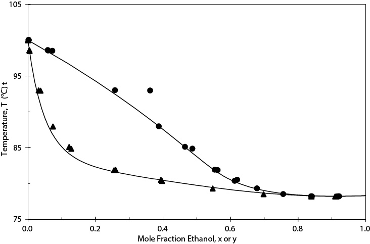
Use the simulator databank BIPs for NRTL to calculate the vapor-liquid equilibrium for ethanol/water at 1 atm. Compare the results for BIPs set to zero. Regress experimental VLE data [12] to determine NRTL BIPs.
Solution
Figure E13.4(a) shows the Txy diagrams using the NRTL BIPs from the CHEMCAD databank and for these BIPs set to zero. Note that the latter case results in an ideal solution; thus, the azeotrope is missed. Regressing the experimental data for this system with the simulator regression tool gives the results shown in Figure E13.4(b). Although the BIPs in the databank (−55.1581, 670.441, 0.3031) and those regressed from the data (−104.31, 807.10, 0.28675) are quite different, the VLE calculated is very similar and is close to the experimental data.

Calculate the LLE for the ternary di-isopropyl-ether/acetic-acid/water using NRTL and the BIPs available for the three binary pairs in the simulator databank. Compare the prediction with ternary LLE data for this system at 24.6°C [13].
Solution
See Figure E13.5. The experimental phase envelope (dotted lines) is twice the size of the predicted one (solid lines). This would lead to gross error in extraction calculations. Note that if all the BIPs are set to zero, there is no liquid-liquid immiscibility region. However, if the ternary LLE data were used to regress all of the BIPs simultaneously, the fit would be quite good.

The recommended strategy for choosing a liquid-state, activity-coefficient model is as follows:
The simulator databank is checked for BIPs for all the binary pairs in the system. If these are available, they are most often from the DECHEMA Data Series [12, 13], but sometimes they are from different sources. Some simulators provide the literature citation; others do not. Each of the three most common models (Wilson, NRTL, UNIQUAC) has different values for BIPs, and they are not correlated from one model to another. Although BIPs for Wilson may not be available for partially immiscible systems (see above), if a binary pair has BIPs for NRTL or for UNIQUAC, the BIPs for that pair should be available for both models. If they are not, the original data are found and the BIPs are fit for the other model.
If phase-equilibrium data can be found for the binary pairs with missing BIPs, a regression is done with the simulator to find the missing BIPs.
For binary pairs that have no measured phase equilibria (there are many!), the UNIFAC estimation option of the simulator is used to estimate the BIPs. There are two UNIFAC methods: one for VLE and one for LLE. The choice depends on the type of equilibrium for the unit operation of interest.
If the unit operation of interest is an extraction or other operation involving LLE or VLLE and ternary data are available, the predictions of the three activity-coefficient models are checked for the ternary LLE.
One of the three methods usually shows a significantly better fit than the others. This method, and the second-best method, are used for the simulation. Comparing the two results provides a rough sense of the uncertainty of the calculation. Note that the “true” result is certainly not guaranteed to be between the two results. It is possible that this strategy will give a false sense of low uncertainty if the two methods give similar predictions that are far from the experimental data. This uncertainty strategy is used in the same way as is any heuristic from Chapter 11. Although this strategy is an analogue of a long-practiced experimental strategy and the basis for numerical analysis error estimation, it does take considerable engineering judgment. Good judgment comes from experience.
If the predictions from the activity-coefficient model chosen do not fit the measured data, a more detailed uncertainty analysis is needed. Although the details of such an analysis are outside the scope of this book, the most important decision is that one is warranted. Calibration of the uncertainty of simulation results is obtained from simulations run with different estimates (high and low, when possible).
The UNIFAC model is never used if experimental data are available for the binary system. UNIFAC is a group-contribution model for determining the BIPs for the UNIQUAC model (and by extension for the NRTL and Wilson models and for equations of state). Only chemical structure data are needed, but the calculations are not very accurate. When determining the numbers of groups within a molecule, the starting point should always be the largest group. This strategy minimizes the assumptions (and therefore the errors) in the model. Group-contribution models should be used with caution.
For many systems, a model such as UNIFAC may be the only option. If so, even a very crude uncertainty estimate can be difficult. If only one phase-equilibrium datum for the system can be found, its deviation from the model prediction is at least some estimate of the uncertainty (as long as that datum was not used to regress parameters).
Using Scarce Data to Calibrate a Thermodynamic Model. Any experimental data on phase equilibria can be used to perform a crude calibration or verification of the model. It need not be the type of data that would be taken in the lab. If the recovery in a column for one set of conditions is known, for example, and if only one BIP is unknown, then the only value of the BIP that will reproduce that datum can be found. Such data are sometimes found in patents.
More Difficult Systems. The above discussions pertain to “easy” systems: (1) small, nonpolar or slightly polar molecules for equations of state and (2) nonelectrolyte, nonpolymeric substances considerably below their critical temperatures for liquid-state activity-coefficient models. Most simulators have some models for electrolytes and for polymers, but these are likely to be even more uncertain than for the easy systems. Again, the key is to find some data, even plant operating data, to verify and to calibrate the models. If the overall recovery from a multistage separation is known, for example, the column can be simulated using the best-known thermodynamic model, and the deviation between the plant datum and the simulator result is a crude (optimistic) estimate of the uncertainty.
Because most thermodynamic options are semitheoretical models for small, nonpolar molecules, the more difficult systems require another degree of freedom in the model. The most common such modification is to make the parameters temperature dependent. This requires additional data, but there is some theoretical justification for using effective model parameters that vary with temperature.
Hybrid Systems. Often a process includes components as wide ranging as solids at room temperature to supercritical gases. They can include water, strong acids, hydrocarbons, and polymers. Often, no single thermodynamic model can be used reliably to predict the fugacities of such a wide range of components. For these cases, simulators allow for hybrid thermodynamic models. The breadth of hybridization varies from one simulator to another, but all at least allow for some components to be considered immiscible with respect to others. For example, the NRTL model may be used for binary pairs for which both compounds are subcritical, while Henry’s Law is used for supercritical (so-called noncondensable) components. Each simulator allows for immiscibility of water and hydrocarbon liquid phases, with the compositions of hydrocarbons in the aqueous phase estimated with Henry’s Law and the liquid-liquid equilibrium for water calculated based on ideal solution in the aqueous phase and some chosen model in the hydrocarbon-rich phase. Each of these options should be checked so that it is clear what the simulator is doing. Although Henry’s Law does not necessarily mean that the phase is aqueous, the Henry’s Law model in a process simulator is often developed only for aqueous systems.
Another kind of hybridization is the choice of auxiliary models for liquid-state activity-coefficient models. The model to use for the vapor phase can be specified and whether to make the Poynting correction. The best choice is to use an equation of state (PR or SRK) for the vapor-phase correction and to use the Poynting correction. Both corrections go smoothly to zero in the low-pressure limit, and neither should add greatly to the computational time for most flowsheets.
The final type of hybridization is the use of different models for different unit operations. Although this appears to be inconsistent at first, it is reality that thermodynamic models are not perfect and that some work much better for LLE than for VLE, some work better for low pressures and others for high pressures, and some work for hydrocarbons but not for aqueous phases. Furthermore, simulators perform calculations for individual units and then pass only component flowrates, temperature, and pressure to the next unit. Thus, consistency is not a problem. Therefore, the possibility of using different models for different unit operations should always be considered. All of the simulators allow this, and it is essential for a complex flowsheet. An activity-coefficient model can be used for the liquid-liquid extractor and an equation of state for the flash unit. This hybridization can be extremely important when, for example, some units contain mainly complex organics and other units contain light hydrocarbons and nitrogen.
Other Models. Different simulators have a variety of additional models beyond those mentioned above. For example, some have nonideal electrolyte thermodynamic models that calculate species equilibria, some have polymer thermodynamic packages, and some allow petroleum cuts to be represented automatically by pseudocomponents. Presently, these packages are less consistent across simulators and are not discussed here. However, the range of models available for the simulator being used should always be investigated.
13.4.4 Using Thermodynamic Models
In summary, the assumed best thermodynamic model should be used, based on the rough guidelines above. However, a process should always be resimulated either with another model assumed to be equally good or with different model parameters (see Example 13.7). The appropriate perturbation to apply to the parameters is available from the experimental data regression or from comparison of calculated results with experimental or plant data. Such data should always be sought for the conditions closest to those in the simulation. If the application is liquid-liquid extraction, for example, liquid-liquid equilibrium data (rather than vapor-liquid equilibrium data) should be used in the parameter regression, even though the same activity-coefficient models are used for both liquid-liquid and vapor-liquid equilibria.
The availability of BIPs in the databank of a process simulator must never be interpreted as an indication that the model is of acceptable accuracy.
These parameter values are merely the “best” for some specific objective function, for some specific set of data. The model may not be able to correlate even these data very well with this optimum parameter set. And one should treat a decision to use a BIP equal to zero as equivalent to using an arbitrary value of the BIP. The decision to use zero is, in fact, a decision to use a specific value based on little or no data.
In simulations of actual processes, there is no substitute for experimental data. No one would invest millions of dollars in a chemical process based on assumed physical properties and phase behavior. In the classroom, a very educated guess may be sufficient to learn the design process, but it must be understood that the actual results are probably not be accurate.
The best thermodynamics method to use is the one that agrees with experimental results.
Consider the DME Tower, T-201, in the DME process in Appendix B. Simulate this unit using a shortcut model with different liquid-state activity-coefficient models to determine the required number of stages for the reflux ratio and the recoveries shown in Appendix B. Include no corrections for heat of mixing. Then perform a rigorous column simulation to check the distillate purity. Compare the results.
The base case uses the UNIFAC model with vapor-phase fugacity correction. The specifications are as follows:
Column pressures: top, 10.3 bar; bottom, 10.5 bar
Key components: light, DME; heavy, methanol
Light key recovery in distillate: 98.93%
Heavy key recovery in bottoms: 99.08%
Reflux ratio: 0.3631
70% plate efficiency
An initial CHEMCAD simulation confirms the value given in Appendix B of 22 actual stages.
Solution
Table E13.6 shows the results obtained from six simulations, all with the same input specifications but with different thermodynamic options. The number of actual stages calculated ranges from 15 to 22; however, the results for two of the simulations (denoted n/a in the table) indicated that the minimum reflux ratio was greater than that specified. Without further information about the ability of the various models to correlate experimental vapor-liquid equilibrium data, a precise solution to the problem is not possible. However, the differences in the results obtained indicate that the choice of thermodynamic model is a crucial one. Of special concern here is the choice of correction of fugacities (denoted w/correction). These corrections are the first and last terms in Equation (13.1). Note that these results were obtained using the CHEMCAD databank BIP values for the NRTL and UNIQUAC models. Different BIP values will yield different results.
Table E13.6 Comparison of Simulations for DME Column, T-201, for Various Thermodynamic Options
Thermodynamic Option |
Number of Actual Stages Obtained from Shortcut Method |
Distillate Purity Obtained with 22 Stages, Specified Reflux Ratio, and Shortcut Reboiler Duty |
Required Reflux Ratio to Obtain DME Purity and Recovery with 22 stages |
Shortcut Method |
Rigorous Simulation |
Rigorous Simulation |
|
UNIFAC w/correction |
22 |
97.3 wt% |
0.52 |
UNIFAC |
15 |
95.0 |
0.47 |
NRTL w/correction |
n/a |
96.6 |
0.77 |
NRTL |
21 |
97.6 |
0.49 |
UNIQUAC w/correction |
n/a |
97.1 |
0.58 |
UNIQUAC |
18 |
97.6 |
0.48 |
To determine which model is best, data on the various binary pairs in the mixture are found. These data consist of measurements of temperature, pressure, and composition of a liquid in equilibrium with its vapor. Sometimes, the concentration of the vapor is also measured. From the temperature and the liquid-phase composition, the pressure and vapor-phase compositions are calculated with the thermodynamic model. The sum of the squared deviations between the experimental and the calculated pressure and between the experimental and the calculated vapor compositions is the objective function. The decision variables are the adjustable parameters in the thermodynamic model. Through the procedures of Chapter 14, the objective function is minimized and the optimum set of parameters is found. The standard process simulators incorporate a tool to do these regressions.
Of great concern is the purity of the overhead product. This stream is the DME product stream from the process, and the specification is 99.5 wt%. The third column in Table E13.6 shows the purity obtained by rigorous, stage-by-stage simulations of this column. In each case, the number of stages, feed location, column pressures, reflux ratio, and reboiler duty were set at those shown in Appendix B. Again, only the thermodynamic option was varied. In the shortcut calculation, many assumptions are made, including the constancy of relative volatilities. For the rigorous calculation, the full power of the thermodynamic package is used in the phase-equilibrium and energy-balance calculations. In this example, the distillate purity specification would be very far off from that calculated with the shortcut method. As expected, the shortcut results are only preliminary to the rigorous column simulation.
The fourth column of Table E13.6 gives the reflux ratio required to meet both the DME purity and recovery specifications. The variation of this ratio from 0.47 to 0.77 is significant, because it is directly related to the required condenser and reboiler duties. If the NRTL w/correction calculation is closest to the truth, the reboiler duty required is 80% greater than that obtained in the baseline shortcut simulation. Ironically, this is the thermodynamics option suggested by the CHEMCAD expert system.
13.5 Case Study: Toluene Hydrodealkylation Process
The purpose of this section is to present the input information necessary to make a basic simulation of the toluene hydrodealkylation process presented in Chapter 1. The required input data necessary to obtain a Level 1 simulation are presented in Table 13.2. The corresponding simulator flowsheet is given in Figure 13.6. In Table 13.2, the equipment numbers given in the third column correspond to those used in Figure 13.6. In the first column, the equipment numbers on the toluene hydrodealkylation PFD (Figure 1.5) are given. It should be noted that there is not a one-to-one correspondence between the actual equipment and the simulation modules. For example, three splitters and six mixers are required in the simulation, but these are not identified in the PFD. In addition, several pieces of equipment associated with the benzene purification tower are simulated by a single simulation unit. The numbering of the streams in Figure 13.6 corresponds to that given in Figure 1.5, except when additional stream numbers are required for the simulation. In order to avoid confusion, these extra streams are assigned numbers greater than 90.
Table 13.2 Required Input Data for a Level 1 Simulation of Toluene Hydrodealkylation Process
Equipment Number |
Simulator Equipment |
Simulator Equip. No. |
Input Streams |
Output Streams |
Required Input |
||
TK-101 |
Mixer |
m-1 |
1 |
11 |
90 |
— |
Pressure drop = 0 bar |
P-101 |
Pump |
p-1 |
90 |
— |
2 |
— |
Outlet pressure = 27.0 bar |
E-101 |
Hexch |
e-1 |
92 |
— |
4 |
— |
Outlet stream vapor fraction = 1.0 |
H-101 |
Heater |
h-1 |
4 |
— |
6 |
— |
Outlet temperature = 600°C |
R-101 |
Stoic react |
r-1 |
93 |
— |
9 |
— |
Conversion of toluene = 0.75 |
E-102 |
Flash |
f-1 |
9 |
— |
8 |
94 |
Temperature = 38°C Pressure = 23.9 bar |
V-101 |
Flash |
f-1 |
9 |
— |
8 |
94 |
No input required because vessel is associated with flash operation |
V-103 |
Flash |
f-2 |
94 |
— |
17 |
18 |
Temperature = 38°C Pressure = 2.8 |
E-103 |
Hexch |
e-2 |
18 |
— |
10 |
— |
Outlet temperature = 90°C |
T-101 |
Shortcut tower |
t-1 |
10 |
— |
19 |
11 |
Recovery of benzene in top product = 0.99 Recovery of toluene in top product = 0.01 R/Rmin = 1.5 Column pressure drop = 0.3 bar |
E-104 |
Shortcut tower |
t-1 |
10 |
— |
19 |
11 |
Included in tower simulation |
E-106 |
Shortcut tower |
t-1 |
10 |
— |
19 |
11 |
Included in tower simulation |
V-102 |
Shortcut tower |
t-1 |
10 |
— |
19 |
11 |
Not required in simulation |
P-102 |
Shortcut tower |
t-1 |
10 |
— |
19 |
11 |
Not required in simulation |
E-105 |
Hexch |
e-3 |
95 |
— |
15 |
— |
Outlet temperature = 38°C |
C-101 |
Compr |
c-1 |
97 |
— |
98 |
— |
Outlet pressure = 25.5 bar |
Mixer |
m-2 |
3 |
5 |
91 |
— |
Pressure drop = 0 bar |
|
Mixer |
m-3 |
2 |
91 |
92 |
— |
Pressure drop = 0 bar |
|
Mixer |
m-4 |
6 |
7 |
93 |
— |
Pressure drop = 0 bar |
|
Mixer |
m-5 |
17 |
96 |
99 |
— |
Pressure drop = 0 bar |
|
Mixer |
m-6 |
99 |
100 |
16 |
— |
Pressure drop = 0 bar |
|
Splitter |
s-1 |
8 |
— |
97 |
96 |
Pressure drop = 0 bar |
|
Splitter |
s-2 |
98 |
— |
5 |
7 |
Pressure drop = 0 bar |
|
Splitter |
s-3 |
19 |
— |
100 |
95 |
Pressure drop = 0 bar |
|
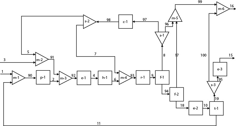
In Table 13.3, the specifications for the feed streams are given. For this process, there are only two feed streams—Streams 1 and 3—corresponding to toluene and hydrogen, respectively. In addition, estimates of all the recycle streams should be given prior to beginning the simulation, and these are given in Table 13.3. However, these estimates need not be very accurate and usually any estimate is better than no estimate at all.
Table 13.3 Feed Stream Properties and Estimates of Recycle Streams
Stream 1 |
Stream 3 |
Stream 11 |
Stream 5 |
Stream 7 |
|
Temperature (°C) |
25.0 |
25.0 |
150.0 |
50.0 |
50.0 |
Pressure (bar) |
1.9 |
25.5 |
2.8 |
25.5 |
25.5 |
Hydrogen (kmol/h) |
— |
286.0 |
— |
200.0 |
20.0 |
Methane (kmol/h) |
— |
15.0 |
— |
200.0 |
20.0 |
Benzene (kmol/h) |
— |
— |
— |
— |
— |
Toluene (kmol/h) |
108.7 |
— |
30.0 |
— |
— |
The data given in Tables 13.2 and 13.3 are sufficient to reproduce the material and energy balances for the toluene hydrodealkylation process. The use of these data to reproduce the flow table in Table 1.5 is left as an example problem at the end of the chapter. As mentioned in Section 13.3, some difficulty may arise when trying to simulate this flowsheet because of the three recycle streams. If problems are encountered in obtaining a converged solution, eliminating as many recycle streams as possible should be tried, following by running the simulation, and then adding recycle streams back into the problem one at a time. The thermodynamic models for this simulation should be chosen using the guidelines in Section 13.4 or using the expert system in the simulator being used. The results given in Chapter 1 for this process were obtained using the SRK models for enthalpy and phase equilibria.
13.6 Electrolyte Systems Modeling
A number of important chemical engineering applications involve electrolytes. Examples of such processes include the following:
Gas-treatment processes. The most common examples are the use of alkanolamines and alkaline-salt solutions for acid-gas removal.
Wastewater treatment for removal of undesired species and for neutralization before disposal. The most common example is the sour-water stripping (SWS) process used primarily for removing NH3 and H2S.
Electrochemical processes. The most common examples include various types of fuel cells, batteries, electrolysis, and corrosion modeling.
Separation processes such as extractive distillation, seawater desalination, and solution crystallization.
Even though it is possible to simulate these systems by writing user-supplied equations, the effort involved to obtain a reasonably accurate model can be significant. With recent advances in process simulators, there are a large number of available models within the simulator that can be customized, and the parameters can be modified to obtain reasonable accuracy. A cursory understanding of the theory of electrolyte systems is necessary for simulating these processes. Therefore, the theory of electrolyte systems will be discussed first along with a discussion of the various available models. These models differ widely in their levels of complexity. After that, the problem of how to set up these models will be discussed through an example. At the end of the chapter, more discussion on electrolyte systems modeling is included for the advanced user.
13.6.1 Fundamentals of Modeling Electrolyte Systems
In chemical processes, electrolyte systems with liquid and vapor phases are very common. These electrolyte models can be readily extended to systems involving solids (such as salts) with suitable modifications. Based on the type of the system, either liquid/liquid equilibrium or solid/liquid equilibrium (such as salt precipitation) must be considered. In an electrolyte system, simultaneous phase and chemical equilibrium calculations are performed.
A strong electrolyte completely dissociates into its constituent ions, whereas a weak electrolyte only partially dissociates. Therefore, a significant amount of the weak electrolyte can remain as molecular species in the solution. There can be one or more solvents in the electrolyte system. Salt precipitation can also occur in such systems. The presence of ions causes highly nonideal behavior in the liquid phase. This impacts both the physical properties as well as the phase and reaction equilibria. Therefore, representative modeling of the chemical and phase equilibria is very important for such systems. Interactions between molecule-molecule, molecule-ion, and ion-ion exist and should be captured in the model. These systems may vary widely because of their chemical compositions (aqueous or mixed solvent, dilute, or concentrated solutions). Their conditions may vary widely, ranging from ambient temperature and pressure to supercritical conditions. While choosing the thermodynamic and transport models, the user must be sure about the applicability of the available models in the process simulator for the particular electrolyte systems being considered. The key considerations are
Is the system aqueous?
Is it a strong electrolyte system?
Is it a mixed-solvent system?
What is the solute concentration?
What is the expected maximum temperature of the system?
In the following discussion, the impact of these questions on the model selection will be covered. The answer to the last question is, of course, the highest temperature in the system, which may occur in a column reboiler or in a fired heater.
There are a number of thermodynamic and transport models available in the open literature. Only some of them are available in process simulators. Most process simulators mention the limitations and applicability of the models in the online documentation. If not, this information can be obtained from the open literature.
The important task of modeling electrolyte systems, as in many other systems, is the calculation of the VLE. Even though the ions do not directly participate in the vapor/liquid equilibrium, they affect the solution properties and the fugacities of the species participating in the equilibrium. For the species in both the phases, the condition for equilibrium is
where ˆfvi
where ˆϕvi,γi,fli
where ϕ*i,P*i,vli
where γ∞i
A number of thermodynamic models are available in the process simulator environment for calculating Gibbs free energy. Table 13.4 provides a quick guideline for the applicability of some of these models, which include models due to Pitzer [14–16], modified Pitzer for systems containing weak electrolytes and molecular nonelectrolytes [17], Bromley-Pitzer [18, 19], electrolyte NRTL (unsymmetric) [20], electrolyte NRTL (symmetric) [21], eNRTL-SAC (unsymmetric) [22], and eNRTL-SAC (symmetric) [23]. The eNRTL-SAC models are particularly applicable to pharmaceutical systems consisting of large, complex molecules along with electrolytes. For sour-water and amine systems, two special thermodynamic models are available in most process simulators. The model for the sour-water system is based on an American Petroleum Institute (API) publication [24]. The model for the amine system, popularly known as “AMINE” or “AMINES,” is mainly based on the Kent-Eisenberg model [25]. This model is used for systems involving amines (mainly monoethanolamine, diethanolamine, diisopropanolamine, diglycolamine) and acid gases (mainly CO2 and H2S). However, some process simulators have extended this model to other amines and other species, along with extensions to a wider operating range. Most process simulators clearly mention the range of operating conditions, such as temperature, pressure, maximum acid-gas loading, and amine concentration, over which the model is expected to be reasonably accurate. For a detailed discussion and additional guidance about using the thermodynamic models mentioned previously, the simulator user manual and the published literature should be consulted. It should be noted that the simulator vendors keep adding new models and updating the parameters for greater accuracy and to enhance the applicability of their model. The discussion above and the data in Table 13.4 are based on currently available capabilities. The simulator documentation is a very good source for these updates. More discussion of the calculation of excess Gibbs energy for electrolyte systems using some of these models can be found in Appendix 13.1.
Table 13.4 Applicability of Some Thermodynamic Models for Calculating Gibbs Free Energy/Activity Coefficient for Electrolyte Systems
Model Name |
Nonaqueous System |
Mixed-Solvent System |
Presence of Molecular Solutes |
Ionic Concentration |
Pitzer |
No |
No |
No |
< 6 molal |
Modified Pitzer |
No |
No |
Yes |
< 6 molal |
Bromley-Pitzer |
No |
No |
No |
< 6 molal |
Electrolyte NRTL (Unsymmetric) |
Yes (but cumbersome and can be inaccurate) |
Yes |
Yes |
Wide range |
Electrolyte NRTL (Symmetric) |
Yes |
Yes |
Yes |
Wide range |
eNRTL-SAC (Unsymmetric) |
Yes (but cumbersome and can be inaccurate) |
Yes |
Yes |
< 6 molal |
eNRTL-SAC (symmetric) |
Yes |
Yes |
Yes |
< 6 molal |
The activity coefficients can be calculated from the excess Gibbs energy. In the molality scale, this is given by
The activity coefficient is then converted to the mole-fraction scale for the VLE calculation. Other thermodynamic properties can be calculated from the excess Gibbs free energy using consistent thermodynamic relationships such as
Thermodynamic relationships similar to Equations (13.7) through (13.10) also hold true for the standard-state properties.
Heat Capacity. The standard-state heat capacities can simply be expressed by a polynomial. If the parameters for such a polynomial are not available for some ionic species, their standard-state heat capacities can be calculated from correlations such as that of Criss and Cobble [26]. According to this correlation, which is based on the “correspondence” principle, partial molal heat capacity of an ionic species is given by
where the parameters Ai(T) and Bi(T) depend upon the ion types and ˉS0i,25
Molar Volume. Even though the molar volume/density can be calculated by thermodynamic relations such as Equation (13.10), this can result in a poor estimate. This information is particularly crucial for plant design and equipment sizing. For estimating the molar volume of an electrolyte system, Equation (13.12) can be written
In Equation (13.12), xw,xs and xel denote the mole fraction of water, all nonwater solvents, and the electrolyte(s), respectively. In addition, vw denotes the molar volume of water that can be obtained from the steam tables, and vs denotes the molar volume of the mixture of all nonwater solvents. The molar volume of nonwater solvents can be found using correlations such as the simple Rackett equation [27], the DIPPR equation [28], or the Campbell-Thodos model [29]. In Equation (13.12), vel denotes the molar volume of the electrolyte that is usually calculated on the basis of the standard state as defined before. One common correlation used in process simulators is due to Redlich and Meyer [30]:
In Equation (13.13), v∞el
Chemical Equilibrium. As the ionic reactions are generally fast, the reactions in an electrolyte system are often treated as equilibrium reactions. However, before performing the chemical equilibrium calculations, all possible reactions in the solutions must be identified. These reactions can be identified from the existing literature or by performing laboratory experiments. Identification of an appropriate reaction set is very important for the electrolyte systems, because the species compositions in the phases depend on both physical and chemical equilibrium. For liquid-phase reactions, the equilibrium constant can be written as
where vi is the stoichiometric coefficient of species i in a reaction, and Keq is the equilibrium constant. Equation (13.14) should be written for all the liquid-phase equilibrium reactions.
In modeling electrolyte systems, transport of reacting species and transport of heat should also be precisely captured. So, the transport models should be selected carefully. The key transport properties are viscosity, thermal conductivity, diffusivity, and surface tension.
Viscosity. For calculating the viscosity of electrolyte systems, the simplest equation is [31]
where μ and μ0 are the viscosities of the electrolyte solution and the pure solvent, respectively, and c is the concentration of electrolyte using a molarity scale. For the case of a mixed-solvent system, μ0 can be calculated by an appropriate model such as the Andrade model [32] or by an appropriate mixing rule. The second term captures the change in the viscosity due to the presence of electrolytes. The coefficient A considers ion-ion interactions and can be calculated by the method of Falkenhagen and Dole [31] based on Debye-Hückel theory. The coefficient A is a function of solvent properties, ionic charges, mobilities, and temperature. However, this equation is applicable only to very dilute systems, up to about 0.01 mol/L. A more widely used equation, which is applicable to solutions with concentrations up to about 0.1 mol/L, is due to Jones and Dole [33]:
The third term on the right-hand side is included to account for the interactions between the solvent and the ions. It should be noted that the solvent-solute interaction can affect the viscosity of the solution. For this reason, the B-coefficient has been studied widely. For more concentrated solutions, a quadratic term was added to Equation (13.16) by Kaminsky [34]. A generic framework that considers similar terms as before was proposed by Lencka et al. [35]. In this speciation-based model, three contributions are considered: a long-range electrostatic term based on the Onsager-Fuoss theory [36], contribution of individual ions, and contribution of interactions between all species (ions and neutral species). This model has proved to be very accurate up to a concentration of 30 mol/kg and up to a temperature of 300°C. Temperature dependence of the parameters used in the viscosity models should also be considered for better accuracy.
Thermal Conductivity. One of the widely used empirical correlations for calculating thermal conductivity of electrolyte solutions is the Riedel equation [37],
where k and k0 are the thermal conductivities of the electrolyte solution and the solvent(s), respectively. αi is the Riedel coefficient for ion i and k0 is calculated by some appropriate correlation or mixing rule for mixed-solvent systems. This equation is accurate for multicomponent systems up to medium concentrations. The Riedel correlation also fails to address the electrolyte systems that exhibit more complicated behavior than the simple linear expression considered in Equation (13.17). A generalized corresponding-states correlation for aqueous binary systems has been proposed by Qureshi et al. [38] using two system-dependent parameters for each binary solution and ten universal parameters. This model is very accurate over a wide range of concentration, pressure, and temperature. Like viscosity models, interactions between solvent-solvent and ion pair–solvent are considered for a mixed-solvent system. One of the key differences with the viscosity model is that the long-range electrostatic interaction term considered in the viscosity model does not have much contribution as derived from the Debye-Hückel-Onsager-Falkenhagen model.
Diffusion Coefficient. Multicomponent diffusion in electrolyte systems plays a key role not only in chemical process technologies but also in a large number of geological systems. For an electrolyte system, diffusivities of both the ions and molecular species need to be calculated. The diffusivities of the molecular species are usually calculated by an appropriate correlation such as that due to Wilke-Chang [39]. If the infinite dilution diffusivity is given by D0 then considering the relaxation effect in an electrolyte solution, the Nernst-Hartley [40] model gives
In Equation (13.18), γ± is the mean ionic activity coefficient and c is the molar concentration. D0 can be calculated from the Nernst equation [41],
where F is Faraday’s constant, z+ and z− are the valences of the ions, and λ0+
In Equation (13.19), a suitable model is required for calculating γ± If the Debye-Hückel model [42] is used, then
where kb is the Boltzmann constant, a is the mean ionic diameter of the electrolyte, εs is the permittivity of the solvent, e is the elementary charge, and 1/κ is the Debye-Hückel length.
where N is Avogadro’s number and I is the ionic strength of the solution. However, this formula may be inaccurate even at concentrations as low as 0.01 N. In concentrated solutions, an additional term has been proposed by Onsager and Fuoss [36] to account for the electrophoretic effect. This effect occurs when the anions and cations migrating in the same direction face the same frictional resistance per ion. At higher concentration, a multiplicative term is introduced that captures the effect of the change in the viscosity on the ionic mobilities at finite concentration. Using the Stefan-Maxwell equation, this approach is found to be valid up to 4 M concentration [43]. The previous discussion again reiterates that a careful selection of the model for calculating diffusivity is required by considering the concentration of the electrolyte system and the number of solvents.
Surface Tension. For calculating surface tension, Onsager and Samaras [44] derived a limiting law neglecting the contribution from the activity coefficient. For a single solute, the limiting law can be written as
where σ0 is the surface tension of the solvent mixture, εr is the relative permittivity of the solvent, and ccc is the concentration of the solute in mole/cm3. σ0 can be calculated using appropriate correlations such as the DIPPR equation [28], an NIST polynomial [45], or by using some mixing rule. For univalent electrolytes, the appropriate relationship can be written as
where cL is the concentration of the solute in mole/L.
Although Equation (13.23), the grand-canonical Onsager-Samaras law based on the Gibbs adsorption isotherm, is very accurate at low concentration (up to about 0.1 M), it underestimates the value of surface tension at higher concentrations. For concentrated solutions, the calculation of surface tension is mainly based on a canonical formalism where the Helmholtz free energy is directly related to the surface tension. For an air-water system, the expression for surface tension takes the following form [46]:
where δ is the thickness of the ion-free layer below the Gibbs dividing surface, and υi and ni are the valence and number density of species i, respectively. λB is the Bjerrum length and is given by λB=e24πεwatkBT,εrat=εair/εwat
Here εair and εwat are the permittivities of air and water, respectively. This formulation shows that the excess surface tension contains a contribution from the ion-free layer, as shown by the second term in Equation (13.24); the image interaction between the electrolyte ions and the ion-free layer, as shown by the third term; and the image interaction between the electrolyte ions and air, as shown by the fourth term. This model is difficult to implement in a process simulator environment without reasonable approximations. To the best of the authors’ knowledge, this formulation is not implemented in any of the leading process simulators. However, it can be implemented in a process simulator as a user model. Discussions of user-added models can be found in Chapter 16, Section 16.2.
13.6.2 Steps Needed to Build the Model of an Aqueous Electrolyte System and the Estimation of Parameters
Multicomponent distillation involving electrolytes is one of the important operations in the chemical process industries. Examples include sour-water strippers, various types of amine-based systems, and alkaline-salt solutions for acid-gas removal. The following discussion concentrates on the simulation of distillation columns involving electrolyte systems. For modeling these systems, not only are the methods and models for the thermodynamic and transport properties important, but also the appropriate unit operation model should be implemented. To obtain a holistic idea of modeling such unit operations, an example of a distillation column will be given and explained. In the example, these property models are used in the overall modeling, and the system of equations that are solved in such systems will be considered. This example will clarify why the thermodynamic and transport models play key roles in the accuracy of the simulation results.
First, a brief review of equilibrium-stage modeling will be given. The equations to be solved are known as the MESH equations [47]. The Material balance equations are written for the n species that are present in the system. Appropriate aqueous-phase ionic reactions are considered as part of this material balance model. The phase-Equilibrium equations depend upon the particular thermodynamic model chosen, as mentioned earlier, and are written for the molecular species. The Summation equations ensure that the mole fractions sum to unity and are written for the liquid and vapor phases. Finally, one entHalpy balance equation is written. It should be noted that if the previous equations are satisfied and the ionic reactions are written properly, the charge balance will be satisfied automatically. Sometimes, for electrolyte systems, an additional constraint due to the charge balance is imposed. Additionally, pressure drop equations may be considered.
In a nonequilibrium-stage modeling problem, the MERSHQ equations are written [47]. In a nonequilibrium-stage model, the mass transfer through the interface plays a key role. For simplicity, consider a two-film model for mass transfer. Here, separate Material balance equations are written for the liquid phase, vapor phase, liquid film, and vapor film. The ionic reactions take place in the liquid phase and usually have very fast kinetics; the reaction terms are usually considered in both the liquid film and the bulk liquid. If additional reactions take place in the vapor phase, those reactions must also be considered. The Energy balance equations are written for the liquid phase, vapor phase, liquid film, and vapor film. At the interface, mass and energy fluxes are considered to be continuous. The transfer Rate equations are written for both mass and energy transfer rates. As before, the Summation equations are written to ensure that the mole fractions sum to unity. The Hydraulic equations are written for calculating the pressure drop across each stage. The phase eQuilibrium equations are written only at the interface as the phase equilibrium is assumed to exist only at the interface. Readers interested in the modeling and theory of multicomponent distillation columns are referred to the text by Taylor and Krishna [47]. Example 13.7 outlines the procedure involved in simulating a multicomponent distillation column. The problem considers the construction of a distillation column model for an electrolyte system in a process simulator using a rate-based simulation with a film model for mass transfer. Some of the steps are also applicable when simulating other unit operations. A detailed generic discussion of these steps, the parameters required at each stage, and possible sources of these parameters are provided in Appendix 13.2 at the end of this chapter.
Develop the model of a sour-water stripper (SWS) as shown in Figure E13.7(a). Consider the following ionic reactions:

For this system do the following:
Simulate both an equilibrium-stage and a nonequilibrium-stage model and compare the key results such as reflux ratio (RR), reboiler duty, and so on.
For comparison, also simulate an equilibrium-stage and a nonequilibrium-stage model without considering the electrolyte chemistry, that is, without the ionic reactions.
Develop another nonequilibrium-stage model without considering the fourth reaction.
The desired specification for the separation is that the bottom product should not have more than 30 ppmw NH3 and 10 ppmw H2S and the top product should have 25% (mole basis) acid gases (H2S and CO2).
Solution
Step 1: Generate the set of linearly independent ionic reactions.
The simulation is set up in Aspen Plus V9.0. It can also be set up in other compatible software platforms. In Aspen Plus V9.0, the “Electrolyte Wizard” can be used to generate a set of possible ionic reactions automatically. The reaction set and the linear independence of the reactions must be checked. In this case, the following equilibrium reactions are generated by selecting hydrogen ion type as H+ and by neglecting salt formation reactions under the “Electrolyte Wizard,” the equilibrium constants are estimated by Aspen Plus V9.0, and these are in agreement with the existing literature:
Here T is in K, the concentration basis is mole fraction, and the reference state for the activity coefficients of ions is chosen to be the aqueous phase at infinite dilution, as mentioned previously. The equilibrium constants are calculated by using reference-state Gibbs free energies of the reactants and products in a particular reaction. In Aspen Plus, the electrolyte calculations can be done with a “true component” or an “apparent component” approach. In this example, the apparent components are H2O, NH3, and H2S. The true components are H2O, H+, OH–, H2S, HS–, S–2, NH3, and NH4+. In this simulation, the “true component approach” is used. For selecting this option, under the “Properties” pane, click the “Home” tab, then click “Methods” on the ribbon. Click the “Global” tab and then check the box for “Use true components” availavle under “electrolyte calculation options.” This option is also available in one of the setup steps in the Electrolyte Wizard.
Step 2: Select the appropriate thermodynamic models and check their parameters.
The electrolyte NRTL (“ElecNRTL” in Aspen Plus V9.0) thermodynamic model is used. Note that NH3 and H2S are considered to be Henry’s Law species. To check the correctness of the thermodynamic model and its parameters, VLE results from the model are compared with the experimental data from Rumpf et al. [48] in Table E13.7(a).
Table E13.7(a) Comparison of the VLE Results from the Simulation with the Experimental Data [48]
Temperature (°C) |
Molality |
pNH3 (MPa) |
pH2S (MPa) |
|||||
NH3 |
H2S |
Exp |
Model |
% Error (abs) |
Exp |
Model |
% Error (abs) |
|
80 |
6.004 |
2.084 |
0.0619 |
0.0669 |
8.08 |
0.0372 |
0.0360 |
3.22 |
80 |
6.033 |
4.647 |
0.0204 |
0.0250 |
22.55 |
0.4231 |
0.4460 |
5.41 |
120 |
5.813 |
2.167 |
0.1660 |
0.1890 |
13.90 |
0.2362 |
0.2709 |
14.70 |
120 |
3.210 |
1.056 |
0.0984 |
0.1023 |
3.96 |
0.1186 |
0.1270 |
7.08 |
Since NH3 and H2S are declared as Henry’s Law species, from Equation (13.13) it can be seen that the VLE calculation depends not only upon the activity coefficients calculated by the electrolyte NRTL model but also on the Henry’s Law constants of the species NH3 and H2S. In Table E13.7(a), it is observed that the VLE results from the simulation are reasonable when compared to the experimental data. Therefore, the default parameters in Aspen Plus for the electrolyte NRTL model and Henry’s Law constants are acceptable and need not be modified. The standard-state heat capacity parameters and the density parameters are not modified since the electrolyte solution is very dilute and it is a weak electrolyte system. So, the standard-state heat capacity and density are not expected to be much different from those of pure water.
Step 3: Select the appropriate transport models and check the parameters.
The default transport models for viscosity, surface tension, thermal conductivity, and diffusivity for the chosen property method are the Jones-Dole model (Equation [13.16]), Onsager-Samaras model (modified Equation [13.22]), Riedel model (Equation [13.17]), and Nernst-Hartley model (Equation [13.18]), respectively. These models with their default settings (option codes in Aspen Plus) and parameters are used because the electrolyte system considered here is very dilute, and these properties are not expected to differ much from those of pure water. For comparison, the surface tension of Stream 1 is compared with the surface tension of pure water and the literature data [49] in Figure E13.7(b).
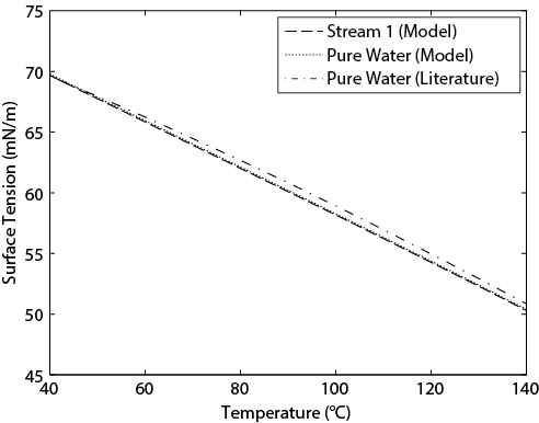
Figure E13.7(b) Surface Tension of Stream 1 and Pure Water from the Aspen Plus Model and Surface Tension of Pure Water from the Literature [49]
Step 4: Set up the distillation column.
First, the equilibrium-stage model is set up by using a “RadFrac” block. The column has 12 stages (including the reboiler and the condenser), the condenser is “partial-vapor,” and the reboiler is “kettle” type. The column condenser pressure is 2 atm (abs), and the pressure drop per stage is 0.007 bar. Stream 1 is specified as given in the problem data and connected to stage 2. Streams 2 and 3 are connected to the condenser and bottom outlets, respectively. Tray sizing is done using single-pass Glitsch ballast-type trays, with the fractional approach to flooding being 0.8. First, a solution is obtained considering a reflux ratio of 2 (mole basis) and bottoms-to-feed ratio (mole basis) of 0.95. At this step, the product specifications are not satisfied, but this step is crucial to take care of any convergence problems and for generating the initial guess for subsequent solutions. The convergence is obtained by using the default “standard” algorithm (an inside-out algorithm). As the H2S specification in the bottom stream can be easily satisfied when the NH3 specification is satisfied, two design specifications are now written to satisfy the product specifications. For maintaining the NH3 specification in Stream 2, its value should be available in the stream results. However, this specification is on an apparent component basis, but this simulation is carried out with the “true component” approach. To calculate the apparent NH3 composition (mass basis) in Stream 2, a user “property set” is set up. To start, under the “Properties” pane, click the “Home” tab, then click “Components” on the ribbon. Click the “Property Sets” on the left-hand side pane. Click “New” and enter a name. In the window that opens up, click the “Properties” tab and then under “Physical properties,” select “WXAPP” from the dropdown options. Under the “Qualifiers” tab, select the “Phase” as “Liquid” and the “Component” as “NH3.” Two “design specs” are written. The first one is to maintain the H2O content in Stream 2 at 75% (mole). The second one is to maintain the NH3 specification in Stream 3. For this, the “design specification type” is selected as “property value,” and under the “property set,” the user property set is selected along with the slection of the appropriate product stream available under the “Feed/Product streams” tab. Two “vary” blocks are created. The “adjusted variables” are “bottoms to feed ratio” and “reflux ratio.” The results are shown in Table E13.7(b).
Table E13.7(b) Comparison of the Key Results from the Equilibrium-Stage Models (with and without Reactions) and the Nonequilibrium-Stage Models
Equilibrium-Stage Model |
Nonequilibrium-Stage Model |
||||
No Reaction |
With Reaction |
No Reaction |
Fourth Reaction Off |
With Reaction |
|
RR (Mole) |
0.52 |
1.60 |
3.94 |
3.94 |
6.82 |
Reboiler Duty (GJ/h) |
23.77 |
25.01 |
27.50 |
27.50 |
30.65 |
Condenser Duty (GJ/h) |
0.55 |
1.7 |
4.17 |
4.17 |
7.23 |
Tray Diameter (m) |
1.36 |
1.39 |
1.44 |
1.44 |
1.51 |
Bottom Temp (°C) |
121.83 |
121.83 |
122.21 |
122.21 |
122.21 |
Bottom Pressure (atma) |
2.07 |
2.07 |
2.10 |
2.10 |
2.10 |
H2S in Bottom (ppmw) |
0 |
1 |
Trace |
Trace |
1.80 |
In the next step, the equilibrium model without the electrolyte chemistry is considered. Note that under this condition, only physical equilibrium is considered. The same thermodynamic model “ElecNRTL” is used, but the electrolyte NRTL model becomes the well-known NRTL model in the absence of ions. The key results are shown in Table E13.7(b).
The nonequilibrium-stage model with the electrolyte chemistry can simply be generated by copying the equilibrium-stage model with the electrolyte chemistry and then modifying it to “rate-based” under “calculation type” available under “specifications.” Here, the condenser pressure is specified, but the pressure drop per tray is removed since it will be calculated. The following tray specifications are used: Glitsch ballast tray with weir height of 46.55 mm. Under “design/Pdrop” in the “setup” menu, the box for “update section pressure profile” is checked and the option for “fix pressure at” is selected as “top.” The box for “rate-based calculations” is checked under “rate-based.” Diffusion resistance in both the liquid and vapor films is considered. Because of the rapid ionic reactions, the reactions are also considered in the liquid film by selecting the option “discrxn.” For determination of mass transfer coefficients, heat transfer coefficients, and interfacial area, the correlations by Gerster et al. [50], Chilton and Colburn [51], and Scheffe and Weiland [52], respectively, are selected under “Tray Rating.” The box for “design mode to calculate column diameter” under “Tray Rating” is checked. The remaining settings are the default values in Aspen Plus V9.0. Again, the design specifications are written after an initial solution is obtained. The differences in the specifications/results are shown in Table E13.7(b). In addition, two other simulations are considered, both using the nonequilibrium-stage model. In the first example, all the reactions are turned off. In the second, only the fourth reaction is turned off. The solution is obtained using the default settings for the solver. Aspen Plus V9.0 solves the rate-based distillation problem using Newton’s method with the solution from the equilibrium-based mode as the initial guess.
In Table E13.7(b), it can be seen that considerable differences exist between the reflux ratios (RR) and condenser duties for all three models. If the nonequilibrium-stage model with all the reactions is considered to be a correct model for the system, then its condenser duty is 4.3 and 13.3 times greater than the equilibrium-stage model with and without reactions, respectively. On the other hand, the results from all three nonequilibrium models show that if the fourth reaction is not considered, the results are similar to the no-reaction case. Even though the electrolyte chemistry is automatically generated in many process simulators when a particular thermodynamic model is chosen, this example demonstrates that the user needs to be vigilant to ensure that all the important reactions are considered. It can be seen in Table E13.7(b) that the H2S concentration in the column bottom stream is well below the required limit of 10 ppmw for all the simulations.
In Example 13.7, the default parameters for the thermodynamic and transport models were used. Because the sour-water system has been well studied for many years and the system is very dilute, the default parameters from Aspen Plus V9.0 are representative. However, for electrolyte systems, where the simulator databank parameters are not available or not representative, the parameters must be regressed, as shown in Example 13.4. More discussion on parameter estimation can be found in Chapter 16, Section 16.5.
13.7 Solids Modeling
Solids handling is abundant in the process industries. Starting from the fluidized catalytic cracking (FCC) unit in a petroleum refinery to the modern power plant using coal, various unit operations involve the handling of solids. Solids may significantly affect mass, momentum, and energy balances in a chemical system even if the solid is inert. In addition, the particle-size distribution of the solid can affect the operation of solid handling equipment such as cyclone separators, crushers and grinders, and crystallizers. Hence, for simulating these processes accurately, the fundamentals of solids modeling must be understood.
13.7.1 Physical Properties
Sections 13.2 and 13.4 provided a detailed account of the importance of selecting the appropriate physical property methods and models. Solids modeling is no exception to this approach. The systems involving solids can be composed of various well-defined solids (such as SiO2, Fe2O3, etc.) or solids that themselves are heterogeneous mixtures of complex materials (such as coal or biomass). In addition, various polymorphs may be present. Polymorphs are different crystalline or amorphous forms of the same solid in which molecules have different arrangements and/or different molecular conformation. The polymorphs usually differ in their dissolution rate, melting temperature, reactivity, sublimation temperature, and other attributes. The properties of the solids depend not only upon their composition but also on their structure, which is almost impossible to characterize in a process simulator. Therefore, many solids that are frequently encountered in the process industries are not available in simulator databanks. Quite often, the user has to declare the solids as a user-defined species, where the needed physical property data are provided. In addition, the thermodynamic and transport calculations that are important for modeling a particular system must be identified. The following discussion considers only systems consisting of nonelectrolyte solids. Systems consisting of electrolyte solids (salts) should be treated as mentioned in Section 13.6.
There are some process operations (such as crystallization) and many metallurgical processes where solid-liquid equilibrium (SLE) is important. In many process simulators, no models exist for calculating SLE. However, in some process simulators, an empirical or semi-empirical approach is available for calculating the SLE. The condition for SLE is
where ˆfli
In terms of activity coefficients, Equation (13.26) can be written as
where ln ψi=∫TTmiHli−HsiRT2dT, zi
For calculating γli
For a multicomponent system, the Margules equation is given by [53]
However, when strong specific interactions such as hydrogen bonding, dimerization, or association exist among some of the constituent molecules, the Margules equation often fails.
There are also a number of systems where solid-vapor equilibrium (SVE) or solid-liquid-vapor equilibrium is important. A sublimation curve may be constructed that represents the SVE on a P-T diagram for pure species. One of the important examples of SVE, being widely studied now, is the formation of gas hydrates or clathrate hydrates. For SVE,
In terms of activity coefficients,
In terms of the Poynting correction factor,
where vsi is the molar volume of the solid for the pure species i. vsi is usually calculated by a polynomial function of temperature, ˆϕvi and ϕ*i can be readily calculated from an equation-of-state model, and γsi is calculated as before. Once γsi is calculated, the excess Gibbs energy for the solid phase can be calculated by
This expression can then be used for methods that use Gibbs energy minimization techniques for equilibrium calculations. Other excess terms can then be calculated using Equations (13.7) through (13.10), as shown in the previous section. For certain chemical processes, the calculation of excess enthalpy is very important and should be checked by regressing with published data.
Similar to electrolyte systems, the standard-state properties can also be calculated by a similar approach. For example, if the standard-state heat capacity (ˉC0p) is known, the standard-state enthalpy, entropy, Gibbs energy, and molar volume can be calculated from similar equations as before.
The standard-state heat capacities can be simply expressed by a polynomial. Pure-component solid heat capacities can be expressed by the suitable DIPPR equations [28], by some polynomial function of temperature, or other standard sources for thermodynamic models and their parameters for pure species [45, 54].
There are some important process applications involving solids that are difficult to characterize in terms of their constituent species. Examples include various types of coal, petroleum cokes, biomass, and other naturally occurring materials. Common processes that involve these solids include combustion, gasification, and reactions involving metal oxides (such as in many chemical looping processes and ore-smelting processes). For such processes, the calculation of enthalpy and density (molar volume) plays a key role. These are usually calculated either from correlations or polynomials. Such formulations are heavily parameterized, and a reasonable estimate of these parameters is needed. Substantial information exists in the open literature that can be used to determine these parameters. The applicability of the form of the model for the solids involved must be checked, and then an estimate of the parameters must be made using regression tools, which are usually available in the process simulator. Parameter estimation using regression tools in a process simulator is discussed in Chapter 16, Section 16.5.
Thermal conductivity of pure solids is often modeled with a polynomial in temperature or using some other correlation. The mixture thermal conductivity is often modeled with a mole- or mass-weighted average or by using a simple mixing rule.
13.7.2 Parameter Requirements for Solids Model
Parameter requirements depend largely upon the system that is being modeled. For example, for a solids combustion system, the enthalpy calculation and the associated parameters must be correct. On the other hand, if a crystallization system is being modeled, the parameter requirements for the SLE calculation must be evaluated carefully. A set of guidelines for choosing the appropriate models and parameters for solids modeling is given:
If the Margules equation is used for calculating the activity coefficients of the species in the solid phase, the A and B parameters are required. These parameters are not composition or pressure dependent, but they are dependent on temperature. Experimental SLE data at different temperatures are needed to determine their temperature dependency. Quite often, these parameters vary with 1/T.
For calculating the fugacity coefficient in the gas phase, interaction parameters may be needed based on the EOS used. Even though these parameters are available in process simulator databanks for a large number of gaseous species, they may not be available for many species that are solid at room temperature. The presence of heterogeneous solids with complex structures will further complicate the situation. These parameters must be determined by regression of experimental data.
As mentioned before, most of the thermodynamic and transport models are empirical for solids systems. The applicability of a model for a particular system should be verified. This can be done by reviewing the existing literature and comparing the model predictions with experimental data in the operating region of interest. If the model parameters are already available in the databank, then the requirement of additional parameters should be checked along with any required modification to the existing parameters. The parameter requirements will depend on the model chosen. The polynomial models, frequently used in solids modeling, are usually linear-in-parameter (LIP) models. Therefore, a least-squares estimate can be obtained easily, even without using the process simulator.
p-Xylene is commercially separated from a mixture of xylenes in a crystallizer, because its freezing point is much higher than that of its other isomers [55]. The feed is first cooled and then sent to a scraped-surface heat exchanger. Since the wall of this heat exchanger is at a very low temperature, the crystals are formed on the wall. These crystals are then removed by scraping with a spring-loaded blade. Two stages are used to increase the product purity. For modeling purposes, only one stage of this process will be considered in this example. This first stage will be modeled as a chiller, E-2001, followed by a crystallizer, CR-2001, as shown in Figure E13.8(a).
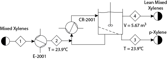
Conditions of Stream 1 in Figure E13.8(a) are as follows:
Temperature (°C) |
23.9 |
|
Pressure (bar) |
1.38 |
|
Flowrate (m3/h) |
16.99 |
|
Composition (wt%) |
||
p-Xylene |
15.8 |
|
m-Xylene |
39.6 |
|
o-Xylene |
20.0 |
|
ethylbenzene |
18.6 |
|
toluene |
6.0 |
|
For simplicity, consider that no recirculation occurs in the crystallizer. The crystal growth rate is given by
where
Xs is the mole fraction of solute in the liquid, and Xs, eq is the mole fraction of solute in the liquid at crystallization temperature. The nucleation rate is given by
Simulate this system and find out the mole fraction of p-xylene in the solvent in Stream 4, the flowrate of solid p-xylene leaving the crystallizer (flowrate of Stream 3), and the supersaturation ratio of Stream 4.
Solution
This system is simulated in PRO/II 8.3. All the species are selected from the SIMSCI databank. For the SLE, the van’t Hoff equation is used. The melting temperature of the species present and the heat of fusion required for the van’t Hoff equation are used from the SIMSCI databank. The solubility of p-xylene calculated by PRO/II matches very well with the experimental data [55], as shown in Figure E13.8(b). Therefore, no changes to the existing PRO/II parameters are necessary for the SLE calculation.
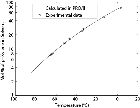
Figure E13.8(b) Comparison of p-Xylene Solubility between Experimental Data [56] and Calculated in PRO/II
Due to the very low temperature of operation and the species in the feed, no vapor phase exists. Therefore, the selection of thermodynamic model for VLE is immaterial. The enthalpy and density calculations are based on generalized correlations available under “library” methods in PRO/II, where the pure species properties are retrieved from the SIMSCI databank. The mole fraction of p-xylene in the solvent in Stream 4 is 0.0607, the flowrate of p-xylene from the crystallizer (flowrate of Stream 3) is 14.37 kmol/h, and the supersaturation ratio of Stream 4 is 5.98 × 10⁻³.
Appendix 13.1
Calculation of Excess Gibbs Energy for Electrolyte Systems
Before discussing the equations for calculating Gibbs free energy, it should be noted that any partial molar property can be written as a departure of that property from the standard state
where ˉM0 and ˉME represent the standard-state and excess properties, respectively. Even though the standard state can be considered to be any defined state, usually a 1 M solution of the species extrapolated to infinite dilution is considered to be the standard state for aqueous electrolyte systems. Therefore, this state is usually called an infinite dilution state. For convenience, the aqueous activity coefficient of a dissolved species is usually defined with an asymmetric convention. With this convention, the activity coefficient approaches unity as the concentration approaches zero.
The molar Gibbs free energy of an electrolyte system can be expressed as
In Equation (13.34), the last term represents the excess Gibbs free energy, μc,w is the chemical potential of pure water, μ∞c,i is the aqueous infinite dilution chemical potential, and the third term on the right-hand side captures the behavior of the species j in an ideal solution. It should be noted that μ∞c,i naturally appears because of the choice of the standard state. Additional terms must be added to the equation if nonaqueous solvents are also present.
If the excess Gibbs energy is represented in terms of activity coefficients, as in Equation (13.34), the nonideal contribution can become a strong function of the model that is chosen for the activity coefficients. The activity coefficients for the electrolyte systems are expressed as a combination of long-range and short-range contribution terms. The long-range contribution represents the interaction in a dilute solution where the solutes are far apart. This term is usually represented by a Debye-Hückel term or a modified Debye-Hückel term. The short-range term is usually represented by summing up the interactions mainly between ion-ion, ion-molecule, and molecule-molecule pairs in a concentrated solution where the solute species are close to each other. Even though a number of formulations are available for calculating the activity coefficients, it is not possible to provide a detailed account of all the models here because of space limitations. However, based on popularity and implementation in commercial process simulators, the work of Pitzer and Chen will be presented here [14, 17, 20]. In most of these models, the excess Gibbs energy is written as
where GexLF and GexSF represent the contribution due to the long-range and short-range forces, respectively. Various expressions are available for capturing the contributions of these forces. The models usually vary because of the different expressions used for capturing these forces. The activity coefficient can be obtained from the excess Gibbs energy from the chosen thermodynamic model. The modified Pitzer equation for excess Gibbs energy of a strong aqueous electrolyte system is [17]
The first term captures the effect of the long-range Coulomb forces. The remaining terms are used to capture the effect of the short-range forces. In Equation (13.36), subscripts c and c′ a and a′ stand for cations and anions, respectively. Z is the absolute value of the ionic charge, nw is the mass of solvent water in kg, and mj represents molality of any solute j. B and θ are binary-interaction terms, and C and ψ represent ternary-interaction terms. The cation-anion interaction parameters B and C are characteristic of single aqueous electrolyte systems, with parameter C being important only at high concentrations. The parameters θ and ψ account for the difference of interaction of the unlike ions of the same sign from the average of the like ions and are characteristics of each aqueous mixed-electrolyte system. f is considered to be a function of the ionic strength. Following Debye-Hückel [42],
where b is a parameter, the optimal value of which is found to be 1.2, and Ix is the ionic strength on a mole fraction basis, where
Aø is the Debye-Hückel constant and is given by
where ds is average solvent density.
As such, the modified Pitzer model does not consider the contribution of the molecular solutes, which is typical for many industrial processes where molecular nonelectrolytes and weak electrolytes are present. These limitations are addressed in the electrolyte-NRTL model [17, 20]. This model captures the short-range interactions similar to the NRTL (nonrandom two-liquid) model. The long-range, ion-ion contributions are captured by the Pitzer-Debye-Hückel model in much the same way as is done in the modified Pitzer equation. This model considers additional terms due to molecule-ion and molecule-molecule interactions and is, therefore, appropriate for weak electrolyte systems. For a multicomponent system, the contribution of the short-range forces due to the excess Gibbs energy is given by the electrolyte-NRTL model as
where subscripts m, c and c′ and a and a′ stand for molecular species, cations, and anions, respectively. Subscripts j and k denote any species.
In Equation (13.40),
Xj = xjLj where Lj = Zj for ions and unity for molecular species
Gji = exp(−αji τji
Gji, ki = exp(−αji, ki τji, ki
α and τ are NRTL nonrandomness and binary-interaction energy parameters, respectively, and x denotes the true liquid-phase mole fraction considering all species. This model is used for both aqueous and mixed-solvent multicomponent electrolyte systems over a wide range of concentrations and temperatures.
Appendix 13.2
Steps to Build a Model of a Distillation Column for an Electrolyte System Using a Rate-Based Simulation with a Film Model for Mass Transfer, the Parameters Required at Each Stage, and Possible Sources of These Parameters
Step 1: Generate the set of linearly independent ionic reactions.
The usual steps for the initial simulator setup for the operating conditions, units of measurement (UOM), and so on, are completed for all the molecular species in the system. In the initial step, it is crucial that all possible ionic reactions be considered. For many process simulators, these reactions are automatically generated. If not, the usual source for obtaining such a reaction set is research literature. Even though a reaction set is automatically generated by the process simulator, it is a good idea to review it and modify it, if needed, based on previous studies reported in the literature.
The equilibrium constants for the ionic reactions are now considered. Usually these constants are automatically calculated by the simulator based on Gibbs energy change or are obtained from some existing databank. If needed, the default values may be changed, based on results in the existing research literature. For the kinetic reactions, usually the pre-exponential factor, activation energy, and exponents on reactions and products must be provided.
At the end of this step, all the species present in the system are generated. If some of the ionic species and their required pure-component properties are not available in the existing simulator databank, then these species must be created and the required pure-component data provided. As discussed in the following paragraphs, the requirement of the pure-component-properties data depends upon the choice of the thermodynamic and transport property models.
Step 2: Select the appropriate thermodynamic models and verify their parameters.
The second important step is the selection of the thermodynamic models. The models should be appropriate for the type of system being modeled. As mentioned, the key property to calculate is the Gibbs free energy of the electrolyte system. Once the model is chosen, the required parameters can be determined by using the data regression system usually available in most process simulators. For example, in the electrolyte NRTL model, the model binary parameters are the nonrandomness factors αca,m, αca,ca′, αca,c′ a, and αmm′ and the energy parameters τca,m, τm,ca, τca,ca′, τca′,ca, τca,c′a, τc′a,ca, τmm′, and τm′m Applying this model to a propanol-water-NaCl system, the binary parameters are αwater-propanol, αNaCl-water, αNaCl-propanol, τNaCl-water, τwater-NaCl, τNaCl-propanol, τpropanol-NaCl, τNaCl-propanol, and τpropanol-water. For the system mentioned above, the parameters αwater-propanol, τwater-propanol, and τpropanol-water can be regressed with LLE data for the propanol-water system. Since data for this aqueous electrolyte systems are abundant, the parameters αNaCl-water, τNaCl-water, and τwater-NaCl can be regressed with data from the NaCl-water system. The remaining three parameters can be found by regression using the mixed-solvent system. Use of the data regression tool in a process simulator environment was discussed earlier in this chapter and will also be discussed later in Chapter 16, Section 16.5. Quite often, only the excess properties are calculated from the excess Gibbs energy, while the standard-state properties are calculated from other thermodynamic properties, such as standard-state heat capacities.
For species that are only slightly soluble, Henry’s Law is often used. The Henry’s constant for at least the key components and solvents must be specified. For a mixed-solvent system, Henry’s Law data are needed for each solvent-species pair. For example, if a system contains two solvents X and Y and two Henry species CO2 and H2S, Henry’s parameter should be supplied for X-CO2, X-H2S, Y-CO2, and Y-H2S. These parameters can be readily calculated from the experimental binary VLE data of the corresponding systems or obtained from handbooks, such as Perry’s handbook [57].
As mentioned before, the standard-state heat capacity may be used for calculating other standard-state properties. If it is calculated from heat capacity polynomials, then the coefficients for such polynomials must be available for all the solvents, the molecular solutes, and the ionic species. In a process simulator, these data are usually available for a large number of molecular solutes and solvents. If the heat capacity is missing for some ionic species, it can be calculated using the Criss-Cobble [26] correlation, as mentioned previously. Next the values for Ai(T), Bi(T), and ˉS0i,25 needed. A large database for heat capacity polynomials or for the Criss-Cobble parameters is available in the open literature [26, 58]. These parameters are usually determined from calorimetric data by considering heats of solution. Data are available for temperatures up to 200°C. Criss and Cobble suggested a simple extrapolation of the entropy parameters beyond 200°C. The validity of such extrapolation needs to be checked on an individual basis. The good news is that most of the common chemical engineering applications with electrolyte systems have operating temperatures below 200°C.
For calculating the molar volume/density, the required parameters should be available and must be appropriate. For example, if the Redlich-Meyer correlation is used for molar volume of the electrolytes, then the values for v∞el, A1, and A2 are required for all the electrolytes present in the system along with the parameters required for calculating molar volume of water and all other solvents. These parameters can be determined by experimental density data of the appropriate systems. For a mixed-solvent system, appropriate parameters are needed for the correlation/mixing law used to calculate the value of vS in Equation (13.12).
Step 3: Select appropriate transport models and verify their parameters.
For some unit operation and equipment models, the transport model may not play any role at all. Usually, this is the result of a simplified model or a simplifying assumption about the transport of the species. For example, if an equilibrium-stage model is developed and the pressure drop is provided by the user, the transport model is probably not used. Sometimes the transport properties are calculated by the simulator for use in the sizing routines.
The viscosity model should be chosen based on the process application. In most viscosity models, in the absence of electrolytes, the viscosity of the pure-solvent/mixed-solvent, μ0 is calculated by an appropriate model. There can be parameter requirements for this model. In addition, model parameters are needed for the correction term. For example, if the Jones-Dole model is chosen for the propanol-water-NaCl system discussed before, the Jones-Dole parameters A and B are needed for the electrolyte NaCl in this mixed-solvent system. Quite often, the coefficients A and B are expressed by some other correlation. In that case, the corresponding parameters are needed. These parameters are usually determined by regressing with experimental viscosity data of binary/ternary systems.
For calculation of the surface tension, if the Onsager-Samaras law is applicable, model parameters will be needed for the appropriate model for calculating σ0 of the pure solvent/solvent mixture. Equation (13.22) is written for a single solute, and for a multicomponent system, an appropriate mixing law can be used. The dielectric constant of the solvent mixture should be calculated with an appropriate law. The correlation for the dielectric constant can have parameters for its temperature dependency. These parameters can be found from experimental data of the solvent mixture and its dielectric properties.
For thermal conductivity, an appropriate model is selected based on the concentration and the particular system being modeled. If the Riedel correlation is used, the Riedel coefficient αi should be known at least for the major species in the solution. These coefficients can be found by regressing with experimental thermal conductivity data.
For calculating diffusivity, an appropriate model should be chosen considering the concentration of the electrolyte system and the number of solvents as mentioned before. If the Nernst-Hartley model is used, parameter a is needed. Usually, the parameters for diffusivity models are regressed with tracer diffusion data.
Step 4: Set up the distillation column simulation.
The appropriate distillation column block is inserted in the simulator, the number of trays is specified (which can be optimized later), the feed(s) is connected, and the feed composition(s) is provided. The feed location(s) is specified, and other column specifications such as pressure, existence of reboiler/condenser, and so forth, are provided. The decision about the appropriate operating pressure is included in the standard textbooks on distillation column design and will not be discussed here. However, the bubble point and dew point calculations required for this purpose can be performed easily in the process simulator. The feed location is evident for some applications. For example, while simulating an absorber, the solvent is fed on the top tray and the feed gas is fed on the bottom tray. In cases where the feed location is not clear, it can be optimized along with the number of trays by using tools readily available in many simulators (such as using the design mode for the shortcut column option). The number of feed trays should be decided considering both the capital and operating costs. For further information, see Chapter 14 on optimization.
The stages on which the ionic reactions take place must be specified. Usually, for an electrolyte system, all the stages including the reboiler and condenser are considered. For very fast reactions using a rate-based distillation column, as would be the case for most ionic reactions, the reactions should be considered to take place in the liquid film as well. The holdup volume of the films is needed to find the reaction rate. For calculating the holdup volume, a correlation is used for a particular type of tray/packing and the tray/packing design details are needed. Many simulators ignore the holdup volume in the downcomers. A simple solution is to use an appropriate scaling factor. Again, if thermodynamic equilibrium is assumed, then the holdup is not important.
For the film model, tray/packing design details are required for calculating mass transfer coefficients and heat transfer coefficients that are used in the mass, equilibrium, rate, and enthalpy equations. One issue is with the determination of the film thickness. For low flux, it can be shown that the film thickness is given by [47]
where ˉD and ˉkm are average diffusivity and mass transfer coefficient, respectively. For calculating the total mass and heat transfer rates in the interface for use in the material (M) balance and energy (E) balance equations for the film region, it is necessary to estimate the interfacial area. For tray columns, the net interfacial area is [47]
where a′ is the interfacial area per unit volume of froth, hf is the froth height, and Ab is the bubbling area. For the packed columns, the net interfacial area is [47]
where a is the interfacial area per unit volume, Ac is the height of a section of packing, and Ac is the cross-sectional area of the column. Appropriate correlations are used for determining a′ In the process simulators, various correlations are available that usually provide the value of the net interfacial area directly for a type of tray/packing. The profile of the calculated interface area can be available depending on the simulator of choice.
For rate-based distillation, the system of equations is usually solved by Newton’s method, by homotopy continuation, or by a combination of both. If the default settings fail to converge, intervention may be required. With Newton’s method, the initial guess plays a strong role in aiding convergence. Process simulators have their own default techniques to generate initial guesses, but these techniques may fail, particularly for electrolyte systems. An estimate of one or more variables, such as pressure, temperature, or compositions, can help convergence. Usually, it is not a good idea to consider some strict design specifications during the first attempt to solve the system. Not only can such design specifications be infeasible due to the current column specification, but they can fail to be realized due to a poor initial guess. Temperature profiles of distillation columns for a number of electrolyte systems are usually available in the open literature and can be used as an initial estimate. Another approach is to solve an equilibrium-stage model first and then use the solution as the initial guess for the nonequilibrium model. The first objective is to get a converged model. Newton’s method requires the calculation of a Jacobian. The partial derivatives of thermodynamic properties are not only very difficult to obtain for the complicated thermodynamic models for electrolytes but are also computationally intensive. More information about the calculation of Jacobians and other related issues can be found in Chapter 16, Section 16.3. Even though the discussion in Section 16.3 concentrates on the solution of the entire flowsheet and in this section the focus is on the solution of a distillation column model for electrolyte systems, many of the issues are similar if Newton’s method or a quasi-Newton method is used.
13.8 Summary
In this chapter, the general components of a process simulator and the seven types of input required to simulate a process successfully were reviewed. Each of the seven required inputs was covered in detail: selection of chemical components, selection of thermodynamic models, selection of process topology, selection of feed stream properties, selection of equipment parameters, selection of output options, and selection of convergence criteria.
Special attention was paid to the role of recycle streams in obtaining converged solutions, and methods to help convergence were discussed. The selection of thermodynamic models and their importance were discussed in depth. A case study for the toluene hydrodealkylation process given in Chapter 1 was given and the required data to complete a process simulation were presented.
Fundamental concepts on electrolyte systems modeling were presented, along with a discussion of the available thermodynamic and transport models in the current process simulators. Further details on the calculation of the Gibbs free energy/activity coefficient were provided in Appendix 13.1. An example was provided to show the steps involved in developing a model of a multicomponent distillation column involving electrolytes. Further discussion of the steps was provided in Appendix 13.2. In Section 13.7, the essentials of solids modeling were discussed. A short discussion on the parameter requirements for solids modeling was provided followed by an example. Overall, this chapter has laid the foundation for developing steady-state simulation using commercial process simulators.
WHAT YOU SHOULD HAVE LEARNED
The typical order for developing a process simulation is as follows:
Select a system of units (such as SI).
Choose the components.
Choose a thermodynamics package.
This must be done carefully.
A thermodynamics package cannot be chosen just because it gives the desired results or simplifies the simulation.
The best package is the one that is confirmed experimentally.
Construct the process by connecting unit operations.
Input the feed stream parameters.
Input the unit operation specifications.
Run the simulation.
For choosing appropriate thermodynamic and transport models for electrolyte systems, the key considerations are the type of system (aqueous versus nonaqueous), what solvents and solutes are present and at what concentration, and the operating temperature.
Quite often, the user has to provide the appropriate physical properties data for solids modeling in the commercial simulators.
Requirement of parameters for solids modeling largely depends upon the system that is being modeled.
References
1. Westerberg, A. W., H. P. Hutchinson, R. L. Motard, and P. Winter, Process Flowsheeting (Cambridge: Cambridge University Press, 1979), ch. 2.
2. Franks, R. G. E., Modeling and Simulation in Chemical Engineering (New York: John Wiley & Sons, 1972), ch. 2.
3. Carnahan, B., H. A. Luther, and J. O. Wilkes, Applied Numerical Methods (New York: John Wiley & Sons, 1969), ch. 5.
4. Elliott, J. R., and C. T. Lira, Introductory Chemical Engineering Thermodynamics, 2nd ed. (Englewood Cliffs, NJ: Prentice Hall, 2012).
5. Sandler, S. I., Chemical, Biological, and Engineering Thermodynamics, 4th ed. (New York: John Wiley & Sons, 2006).
6. Smith, J. M., H. C. Van Ness, and M. M. Abbott, Introduction to Chemical Engineering Thermodynamics, 7th ed. (New York: McGraw-Hill, 2005).
7. Soave, G., “Equilibrium Constants from a Modified Redlich-Kwong Equation of State,” Chem. Eng. Sci. 27 (1972): 1197.
8. Redlich, O., and J. N. S. Kwong, “On the Thermodynamics of Solutions: V. An Equation of State: Fugacities of Gaseous Solutions,” Chem. Rev. 44 (1949): 233.
9. Horwitz, B. A., and A. J. Nocera, “Are You ‘Scotamized’ by Your Simulation Software?” CEP 92, no. 9 (1996): 68.
10. Schad, R. C., “Don’t Let Recycle Streams Stymie Your Simulations,” CEP 90, no. 12 (1994): 68.
11. Whiting, W. B., “Effects of Uncertainties in Thermodynamic Data and Models on Process Calculations,” J. Chem. Eng. Data. 41 (1996): 935.
12. Gmehling, J., and U. Onken, Vapor-Liquid Equilibrium Data Collection (Frankfurt am Main, Germany: DECHEMA, 1977).
13. Sorensen, J. M., and W. Arlt, Liquid-Liquid Equilibrium Data Collection (Frankfurt am Main, Germany: DECHEMA, 1979).
14. Pitzer, K. S., “Thermodynamics of Electrolytes: I. Theoretical Basis and General Equations,” J. Phys. Chem. 77 (1973): 268–277.
15. Pitzer, K. S., and J. S. Kim, “Thermodynamics of Electrolytes: IV. Activity and Osmotic Coefficients for Mixed Electrolytes,” J. Am. Chem. Soc. 96 (1974): 5701–5707.
16. Pitzer, K. S., “Thermodynamics of Electrolytes: V. Effects of Higher Order Electrostatic Terms,” J. Solution Chem. 4 (1975): 249–265.
17. Chen, C., H. Britt, J. Boston, and L. Evans, “Extension and Application of the Pitzer Equation for Vapor-Liquid Equilibrium of Aqueous Electrolyte Systems with Molecular Solutes,” AIChE J. 25 (1979): 820–831.
18. Fürst, W., and H. Renon, “Effects of the Various Parameters in the Application of Pitzer’s Model to Solid-Liquid Equilibrium: Preliminary Study for Strong 1-1 Electrolytes,” Ind. Eng. Chem. Process Des. Dev. 21 (1982): 396–400.
19. Bromley, L. A., “Thermodynamic Properties of Strong Electrolytes in Aqueous Solution,” AIChE J. 19 (1973): 313–320.
20. Chen, C., and L. B. Evans, “A Local Composition Model for the Excess Gibbs Energy of Aqueous Electrolyte Systems,” AIChE J. 32 (1986): 444–454.
21. Song, Y., and C. Chen, “Symmetric Electrolyte Nonrandom Two-Liquid Activity Coefficient Model,” Ind. Eng. Chem. Res. 48 (2009): 7788–7797.
22. Chen, C., and Y. Song, “Extension of Nonrandom Two-Liquid Segment Activity Coefficient Model for Electrolytes,” Ind. Eng. Chem. Res. 44 (2005): 8909–8921.
23. Song, Y., and C. Chen, “Symmetric Nonrandom Two-Liquid Segment Activity Coefficient Model for Electrolytes,” Ind. Eng. Chem. Res. 48 (2009): 5522–5529.
24. API Publication 955, “New Correlation of NH3, CO2 and H2S Volatility Data from Aqueous Sour Water System,” March 1978, http://www.api.org/Publications/.
25. Kent, R. L., and B. Eisenberg, “Better Data for Amine Treating,” Hydrocarbon Processing 55 (1976): 87–90.
26. Criss, C. M., and J. W. Cobble, “The Thermodynamic Properties of High Temperature Aqueous Solutions: V. The Calculation of Ionic Heat Capacities Up to 200°. Entropies and Heat Capacities above 200°,” J. Am. Chem. Soc. 86 (1964): 5390–5393.
27. Rackett, H. G., “Equation of State for Saturated Liquids,” J. Chem. Eng. Data 15 (1970): 514–517.
28. Rowley, R. L., W. V. Wilding, J. L. Oscarson, N. A. Zundel, T. L. Marshall, T. E. Daubert, and R. P. Danner, DIPPR Data Compilation of Pure Compound Properties (New York: Design Institute for Physical Properties, AIChE, 2002).
29. Campbell, S. W., and G. Thodos, “Prediction of Saturated-Liquid Densities and Critical Volumes for Polar and Nonpolar Substances,” J. Chem. Eng. Data. 30 (1985): 102–111.
30. Redlich, O., and D. Meyer, “The Molal Volumes of Electrolytes,” Chem. Rev. 64 (1964): 221–227.
31. Falkenhagen, H., and M. Dole, “Die innere Reibung von Elektrolytischen Losungen und ihre Deutung nach der Debyeschen Theorie,” Phys. Z. 30 (1929): 611–622.
32. Andrade, E. N. da C., “The Viscosity of Liquids,” Nature 125 (1930): 309–310.
33. Jones, G., and M. Dole, “The Viscosity of Aqueous Solutions of Strong Electrolytes with Special Reference to Barium Chloride,” J. Am. Chem. Soc. 51 (1929): 2950–2964.
34. Kaminsky, M., “The Concentration and Temperature Dependence of the Viscosity of Aqueous Solutions of Strong Electrolytes: III. KCl, K2SO4, MgCl2, BeSO4, and MgSO4 Solutions,” Z. Phys. Chem. 12 (1957): 206–231.
35. Lencka, M. M., A. Anderko, S. J. Sanders, and R. D. Young, “Modeling Viscosity of Multicomponent Electrolyte Systems,” Int. J. Thermophys. 19 (1998): 367–378.
36. Onsager, L., and R. Fuoss, “Irreversible Processes in Electrolytes: Diffusion, Conductance, and Viscous Flow in Arbitrary Mixtures of Strong Electrolytes,” J. Phys. Chem. 36 (1931): 2689–2778.
37. Riedel, L., “Die Wärmeleitfähigkeit von wässrigen Lösungen starker Elektrolyte,” Chem. Ing. Tech. 23 (1951): 59–64.
38. Qureshi, A. S., P. Ravi, Y. P. Doshi, and S. Murad, “Generalized Corresponding States Correlations for the Viscosity and Thermal Conductivity of Aqueous Electrolyte Solutions,” Chem. Eng. Commun. 136 (1995): 27–44.
39. Wilke, C. R., and P. Chang, “Correlation of Diffusion Coefficients in Dilute Solutions,” AIChE J. 1 (1955): 264–270.
40. Hartley, G., “Theory of the Velocity of Diffusion of Strong Electrolytes in Dilute Solution,” The London, Edinburgh and Dublin Phil. Mag. J. Sci. 12 (1931): 473–488.
41. Nernst, W., “Zur Kinetik der in Lösung befindlichen Körper: I. Theorie der Diffusion,” Zeitschrift für Physikalische Chemie 2 (1888): 613–637.
42. Debye, P., and E. Hückel, “The Theory of Electrolytes: I. Lowering of Freezing Point and Related Phenomena,” Physik. Z. 24 (1923): 185–206.
43. Pinto, N., and E. E. Graham, “Evaluation of Diffusivities in Electrolyte Solutions Using Stefan-Maxwell Equations,” AIChE J. 32 (1986): 291–296.
44. Onsager, L., and N. N. T. Samaras, “The Surface Tension of Debye-Hückel Electrolytes,” J. Chem. Phys. 2 (1934): 528–536.
45. Chase, M. W., NIST-JANAF Thermochemical Tables, 4th ed., J. Phys. Chem. Ref. Data, Monogr., Vol. 9 (NJ: Springer, 1998).
46. Ohshima, H., “Surface Tension of General Electrolyte Solutions,” Colloid Polym. Sci. 283 (2004): 119–124.
47. Taylor, R., and R. Krishna, Multicomponent Mass Transfer (New York: John Wiley & Sons, 1993).
48. Rumpf, B., Á. Kamps, R. Sing, and G. Maurer, “Simultaneous Solubility of Ammonia and Hydrogen Sulfide in Water at Temperatures from 313 K to 393 K,” Fluid Phase Equilibria 158–160 (1999): 923–932.
49. Vargaftik, N. B., B. N. Volkov, and L. D. Voljak, “International Tables of the Surface Tension of Water,” J. Phys Chem. Ref. Data 12 (1983): 817–820.
50. Gerster, J. A., A. B. Hill, N. N. Hochgraf, and D. G. Robinson, “Tray Efficiencies in Distillation Columns,” Final Report of University of Delaware, (New York: AIChE, 1958).
51. Chilton, T. H., and A. P. Colburn, “Mass Transfer (Absorption) Coefficients,” Ind. Eng. Chem. 26 (1934): 1183–1187.
52. Scheffe, R. D., and R. H. Weiland, “Mass Transfer Characteristics of Valve Trays,” Ind. Eng. Chem. Res. 26 (1987): 228–236.
53. O’Connell, J. P., and J. M. Haile, Thermodynamics: Fundamentals for Applications (New York: Cambridge University Press, 2005).
54. Barin, I., Thermochemical Data of Pure Substances, Parts I and II, 3rd ed. (Germany: Wiley-VCH, 1997).
55. Haines, H. W., Jr., J. M. Powers, and R. B. Bennett, “p-Xylene from Petroleum,” Ind. Eng. Chem. 47 (1955): 1096–1103.
56. Haddon, W. F., Jr., and J. F. Johnson, “Solubility Data for p-Xylene,” J. Chem. Eng. Data 9 (1964): 158–159.
57. Perry, R. H., D. W. Green, and J. O. Maloney, eds., Perry’s Chemical Engineers’ Handbook, 7th ed. (New York: McGraw-Hill, 1997).
58. Hepler, L. G., and J. K. Hovey, “Standard State Heat Capacities of Aqueous Electrolytes and Some Related Undissociated Species,” Can. J. Chem. 74 (1996): 639–649.
59. Mandal, B. P., M. Guha, A. K. Biswas, and S. S. Bandyopadhyay, “Removal of Carbon Dioxide by Absorption in Mixed Amines: Modelling of Absorption in Aqueous MDEA/MEA and AMP/MEA Solutions,” Chem. Eng. Sci. 56 (2001): 6217–6224.
60. Austgen, D. M., G. T. Rochelle, X. Peng, and C. Chen, “Model of Vapor-Liquid Equilibria for Aqueous Acid Gas-Alkanolamine Systems Using the Electrolyte-NRTL Equation,” Ind. Eng. Chem. Res. 28 (1989): 1060–1073.
Short Answer Questions
1. In the activity-coefficient model of an electrolyte system, how is the effect of the long-range forces included?
2. Even though the ions do not directly participate in the VLE of an electrolyte system, why does their presence affect the VLE of an electrolyte system?
3. The reboiler temperature of an electrolyte process is known to be 150°C–200°C. One of the species present in this system is H2S. How would you model the fugacity of H2S in the liquid phase?
4. An electrolyte NRTL model is used for VLE calculation of a strong electrolyte system consisting of four species. How many binary interaction parameters are needed? What are they?
5. You are developing an equilibrium-stage model of a distillation column with fixed pressure drop in an electrolyte system. Is the model for surface tension important? Explain.
6. A model of biomass combustion in an industrial furnace is to be developed. Calculation of which thermodynamic property is the most important?
Problems
7. For the toluene HDA process, using the data given in Tables 13.1 and 13.2, simulate the process and compare the results with those given in Chapter 1, Table 1.5. Remember that the number of actual plates is given in Table 1.7, and an efficiency of 0.6 was assumed.
8. For the DME flowsheet given in Appendix B, Figure B.1.1, list the minimum input information required to obtain mass and energy balances for this process. Using the process simulator available to you, simulate the DME process and compare your results to those given in Table B.1.1.
9. For the isopropyl alcohol to acetone process flowsheet given in Appendix B, Figure B.10.1, list the minimum input information required to obtain mass and energy balances for this process. Using the process simulator available to you, simulate the isopropyl alcohol to acetone process, and compare your results to those given in Table B.10.1.
10. Using the results from Problem 13.7 and Tables 1.5 and 1.7, compare the results for the simulation of the benzene recovery column, T-101, using a shortcut method and a rigorous method. One way to do this comparison is to use the number of theoretical plates from the shortcut method as an input to the rigorous method. The rigorous method is used to simulate the same separation as the shortcut method, that is, the same overhead purity and recovery. The difference in the methods is then reflected by the difference between the reflux required for both methods. Comment on the difference for this nearly ideal system. Remember that there is no need to simulate the whole flowsheet for this problem; just use the input to the column from Table 1.5.
11. In Problem 13.7, you should have simulated the reactor as a stoichiometric reactor with 75% per pass conversion. In order to estimate the volume of the reactor, it is necessary to have kinetics expressions. For the catalytic hydrodealkylation of toluene, assume that the reaction is kinetically controlled with the following kinetics:
where
With these kinetics, simulate the reactor in Figure 1.5 as a two-stage packed-bed adiabatic reactor with a “cold shot” (Stream 7) injected at the inlet to the second bed. The maximum temperature in the reactor should not exceed 655°C, and this will occur at the exit of both beds; that is, design the system for this maximum outlet temperature for both packed beds. Compare your results with the total volume of the catalyst given in Table 1.7.
12. As noted in Section 13.5, the results provided for the toluene hydrodealkylation process are based on the SRK model for both enthalpy and phase equilibria. Determine the BIPs for this model used by the simulator available to you. If you have access to more than one simulator, compare the BIPs from each. Simulate the benzene column (T-101) using the shortcut simulation module and the specifications given in Table 13.2 and the conditions of feed stream (10) given in Example 13.2. Rerun the simulation with all the BIPs set to zero. Compare the results.
13. Determine what thermodynamic models were used for each of the processes in Appendix B. Explain why each was chosen, and give at least one other thermodynamic model that is reasonable and should be tried for each process.
14. For the system DME/methanol/water, determine the BIPs used in the simulator available to you for each of these thermodynamic models: NRTL, Wilson, and UNIQUAC. Simulate T-202 using a shortcut module for each of these models, and compare the number of theoretical stages required for the specified recoveries and R/Rmin = 1.5.
15. Find VLE data in the literature for the system methanol/water. Regress these data to determine the BIPs for the UNIQUAC model. Compare the results of these with the results obtained using the BIPs available in the simulator databank and with the results obtained using the UNIFAC model.
16. Using the Henry’s Law model in the simulator available to you, determine the concentration of oxygen (ppm by mass) in water at 25°C and at 35°C if the water is in equilibrium with air. Compare the results obtained to those calculated using the PR model with the BIPs available in the simulator databank.
17. Using the help facility of the simulator available to you, determine how the simulator handles VLE calculations with supercritical components when an activity-coefficient model is specified. (Note that P*i in Equation 13.1 is undefined for these components.)
18. For the ethylbenzene flowsheet given in Appendix B, Figure B.2.1, list the minimum input information required to obtain mass and energy balances for this process. Using the process simulator available to you, simulate the ethylbenzene process and compare your results to those given in Table B.2.1.
19. For the styrene flowsheet given in Appendix B, Figure B.3.1, list the minimum input information required to obtain mass and energy balances for this process. Using the process simulator available to you, simulate the styrene process and compare your results to those given in Table B.3.1.
20. For the maleic anhydride flowsheet given in Appendix B, Figure B.5.1, list the minimum input information required to obtain mass and energy balances for this process. Using the process simulator available to you, simulate the maleic anhydride process and compare your results to those given in Table B.5.1.
21. For the ethylene oxide flowsheet given in Appendix B, Figure B.6.1, list the minimum input information required to obtain mass and energy balances for this process. Using the process simulator available to you, simulate the ethylene oxide process and compare your results to those given in Table B.6.1.
22. For the formalin flowsheet given in Appendix B, Figure B.7.1, list the minimum input information required to obtain mass and energy balances for this process. Using the process simulator available to you, simulate the formalin process and compare your results to those given in Table B.7.1.
23. Investigate the batch aspects of the simulator available to you. Remember that these could include reactor, separation, and scheduling modules as well as others.
24. Determine which thermodynamic models were used for each of the processes in Appendix B. Explain why each was chosen, and give at least one other thermodynamic model that is reasonable and should be tried for each process.
25. Using the Henry’s Law model in the simulator available to you, determine the concentration of oxygen (ppm by mass) in water at 10°C and 27°C if the water is in equilibrium with air. Compare the results obtained to those calculated using the SRK model with the BIPs available in the simulator databank.
26. As noted in Section 13.5, the results provided for the toluene hydrodealkylation process are based on the SRK model for both enthalpy and phase equilibria. Simulate the benzene column (T-101) with the PR model instead, using the shortcut simulation module and the specifications given in Table 13.2 and the conditions of feed stream (10) given in Example 13.2. Determine the BIPs for the PR model used by the simulator. Rerun the simulation with all the BIPs set to zero. Compare the results.
27. Figure P13.27 is the absorber in an acid-gas removal (AGR) plant.
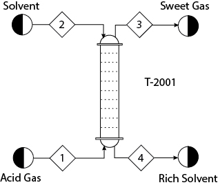
The solvent, Stream 2, in this plant is a chemical solvent, methyl diethanolamine (MDEA). It is fed to the top of the column. The acid gas, Stream 1, is fed to the bottom of the column. The conditions of Streams 1 and 2 are given in Table P13.27. The column has 20 theoretical stages. Simulate an equilibrium-stage model of this column considering the important ionic reactions and a suitable thermodynamic model for this electrolyte system. The column top pressure is 1.6 atm. Consider the following reactions [59, 60]:
Table P13.27 Feed Stream Data for Problem 13.27
Stream 1 |
Stream 2 |
|
Temperature (°C) |
38.0 |
38.0 |
Pressure (atm) |
1.8 |
1.6 |
Total Flow (kmol/h) |
47.33 |
61.19 |
Composition (mol%) |
||
H2O |
4.2 |
84.7 |
CO2 |
10.5 |
0.022 |
H2S |
1.7 |
6.0 × 10⁻⁵ |
CH4 |
2.5 |
— |
N2 |
49.5 |
— |
O2 |
0.1 |
— |
CO |
18.9 |
— |
H2 |
12.6 |
— |
MDEA |
— |
15.3 |
What are the compositions and temperatures of Stream 3 and Stream 4?
28. Consider the same problem as Problem 13.27, but now develop a nonequilibrium-stage model with 20 theoretical stages. The first two reactions shown in Problem 13.27, even though reversible, are kinetically limited, while the rest of the reactions can be considered to be fast and at equilibrium. Consider using single-pass valve trays with the appropriate diameter (which can be calculated by the process simulator—assume 80% of flooding) and 152 valves/m2 of active area. Consider a tray spacing of 0.6096 m and a weir height of 46.55 mm. Fix the top pressure at 1.6 atm and calculate the pressure drop through the entire column. Depending on the process simulator available to you, consider appropriate transport models and account for the mass transfer resistance in both the liquid and vapor films. Since the related ionic reactions are very fast, consider that the ionic reactions also take place in the liquid film. Compare the results for Streams 3 and 4 with the results from Problem 13.27.
29. Consider Problem 13.28. The solvent MDEA becomes rich in acid gases. To recycle this solvent, it is first heated to 90°C in exchanger E-2001 and then sent to the top stage of the stripper T-2002 as shown in Figure P13.29. Develop a nonequilibrium-stage model of the stripper with 20 theoretical stages, a partial-vapor condenser, and a kettle-type reboiler. Reflux ratio (mole basis) = 0.7 and bottoms/feed ratio (mole basis) = 0.97. The pressure in the condenser is 1.4 atm, and the pressure drop through the entire column should be calculated. Consider the ionic reactions in all the stages, including the condenser and reboiler. It can be assumed that all ionic reactions reach equilibrium in the condenser and reboiler because of the longer residence times. Assume that the tray hardware is similar to the absorber. The mass transfer and the ionic reactions in the liquid and vapor films can be modeled similarly to Problem 13.28. For this problem determine the following:
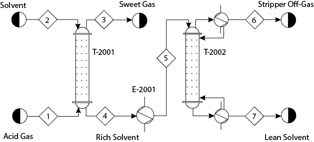
What are the duties of the stripper and reboiler?
What are the compositions of Streams 6 and 7?
What operating condition(s) of the stripper would you change if you wanted to increase the purity of Stream 7?
30. Develop a model of a coal combustor fed with Illinois No. 6 coal, a bituminous coal, at 2 atm pressure. The atmospheric air for combustion is available at a temperature of 150°C. The flow of combustion air is 10% more than the stoichiometric requirement. The coal is also available at 150°C. The composition for Illinois No. 6 coal is
Proximate Analysis (wt%) |
|
Moisture |
11.12 |
Ash |
9.70 |
Volatile Matter |
34.99 |
Fixed Carbon |
44.19 |
Ultimate Analysis (wt%) |
|
Moisture |
11.12 |
Carbon |
63.75 |
Hydrogen |
4.50 |
Nitrogen |
1.25 |
Chlorine |
0.29 |
Sulfur |
2.51 |
Ash |
9.70 |
Oxygen |
6.88 |
The combustor is adiabatic. Assume the carbon conversion to be 100%. The high heating value (HHV) of the coal is reported to be 27,113 kJ/kg. Compare the heating value estimated by the process simulator with this reported value. As mentioned before, most of the models for heterogeneous solids are empirical. Modify the parameters of the enthalpy model to match the reported heating value. What is the composition at the outlet of the combustor?
31. A biomass stream, Stream 1 in Figure P13.31, is being dried in a direct dryer, V-2001, by a stream of hot N2. Develop a model for this dryer. The composition of Stream 1 (wt%) is
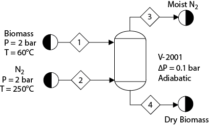
Cellulose |
55.0 |
Hemicellulose |
15.0 |
Lignin |
12.5 |
Moisture |
15.0 |
Ash |
2.5 |
The ash can be considered to be pure calcium oxide (CaO). The flowrate of biomass is 500 kg/min. Assume adiabatic operation in V-2001 with a pressure drop of 0.1 bar. What models would be appropriate for the solids density and enthalpy calculations? If the model parameters are not available for the biomass components in the simulator of your choice, use values from the open literature. The desired moisture content of Stream 4 is 1% (wt). As many commercial process simulators do not have the capability to model the SVE for such processes, assume that the desired moisture content is achieved at 110°C. What is the required flowrate of N2?
32. Wood pellets, Stream 1 in Figure P13.32, are first dried by indirect heating with the flue gas and then combusted. Model this system using a heat exchanger, E-2001, followed by a flash separator, V-2001. The dried wood pellets are combusted in an adiabatic combustor, R-2001, where combustion air is supplied in 15% excess of the stoichiometric requirement. The hot flue gas is used for raising steam in a boiler. The boiler can be simply modeled as a heat exchanger where the flue gas is cooled to 300°C. The flue gas then exchanges heat in E-2001 before being vented through the stack. For simplicity consider the pressure drop through each piece of equipment to be 0.1 bar. The composition of wood pellets is

Proximate Analysis (wt%) |
|
Moisture |
8.80 |
Ash |
2.40 |
Volatile Matter |
73.00 |
Fixed Carbon |
15.80 |
Ultimate Analysis (wt%) |
|
Moisture |
8.80 |
Carbon |
47.00 |
Hydrogen |
5.00 |
Nitrogen |
0.49 |
Sulfur |
0.08 |
Ash |
2.40 |
Oxygen |
36.23 |
The HHV of the wood pellets is 18,969 kJ/kg. Feel free to include additional blocks in the process simulator that you need to use to model the combustor operations appropriately. Assume the conversion of carbon to be 100%. As many commercial process simulators do not have the capability to model the SVE for such processes, assume that 90% of the moisture in the feed is separated in the dryer (i.e., leaves in Stream 3).
What are the temperatures of Streams 2, 4, and 7?
What is the composition of Stream 7?
Perform an overall energy analysis of this system and compare with the reported HHV. Modify the parameters of the enthalpy model to match the HHV.